
Annual and Seasonal Patterns of Burned Area Products in Arctic-Boreal North America and Russia for 2001–2020

 ,
,  , , , , ,
  , and
, and
Abstract
:1. Introduction
2. Methodology
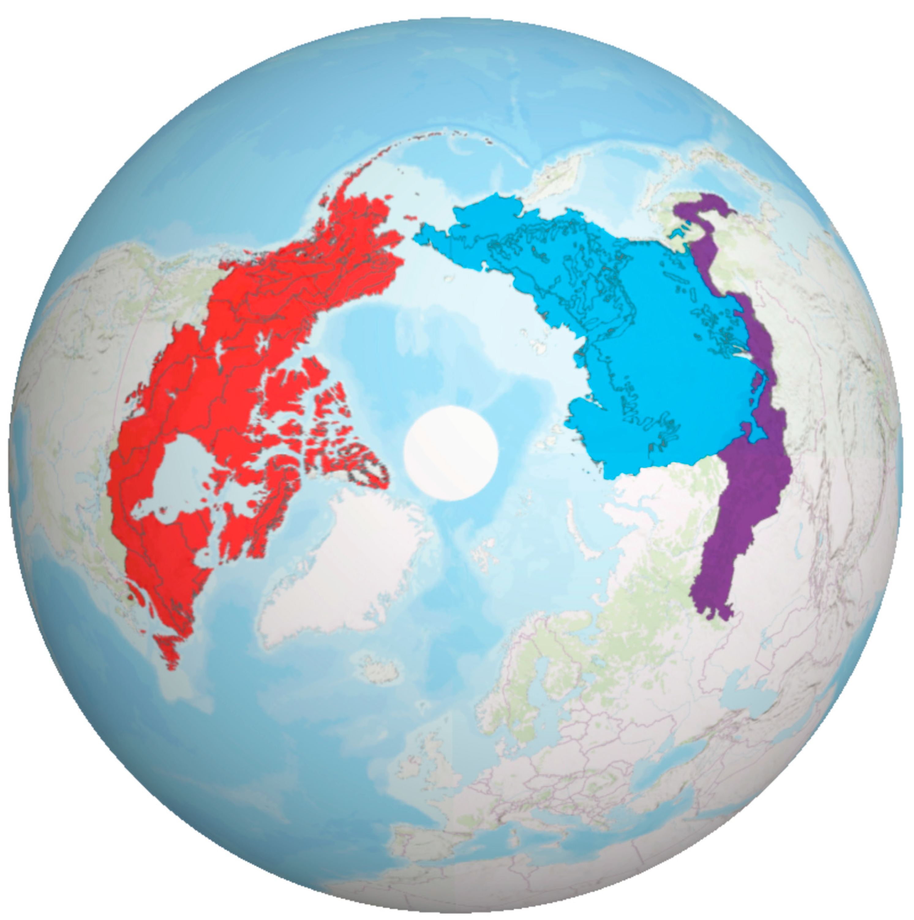
2.1. Study Areas
2.2. Datasets
2.2.1. FireCCI51
2.2.2. MCD64A1
2.2.3. GABAM
2.2.4. GFED4s
2.2.5. GFED5
2.2.6. FireCCILT11
2.2.7. MTBS
2.2.8. NBAC
2.2.9. ABoVE-FED
2.2.10. SRBA
2.2.11. Talucci et al. Fire Perimeter Product
2.2.12. ABBA
2.2.13. MODIS Active Fires
2.3. Analysis Techniques
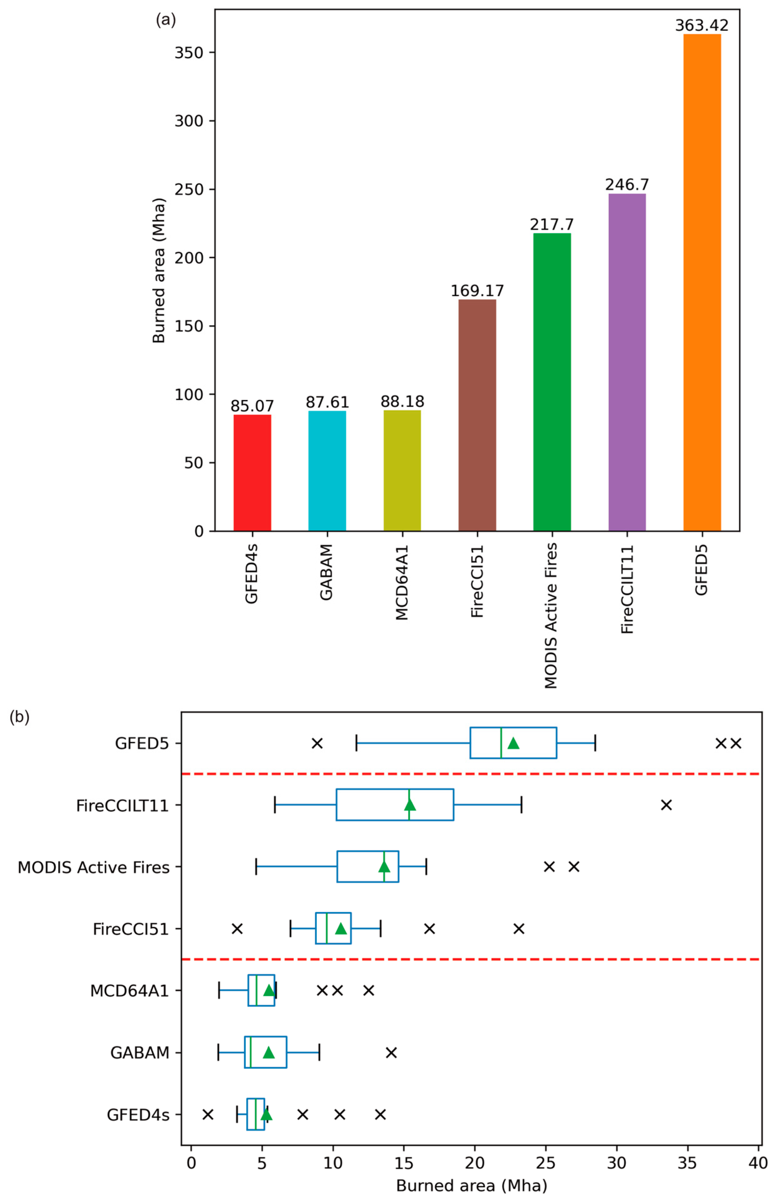
2.3.1. Yearly BA
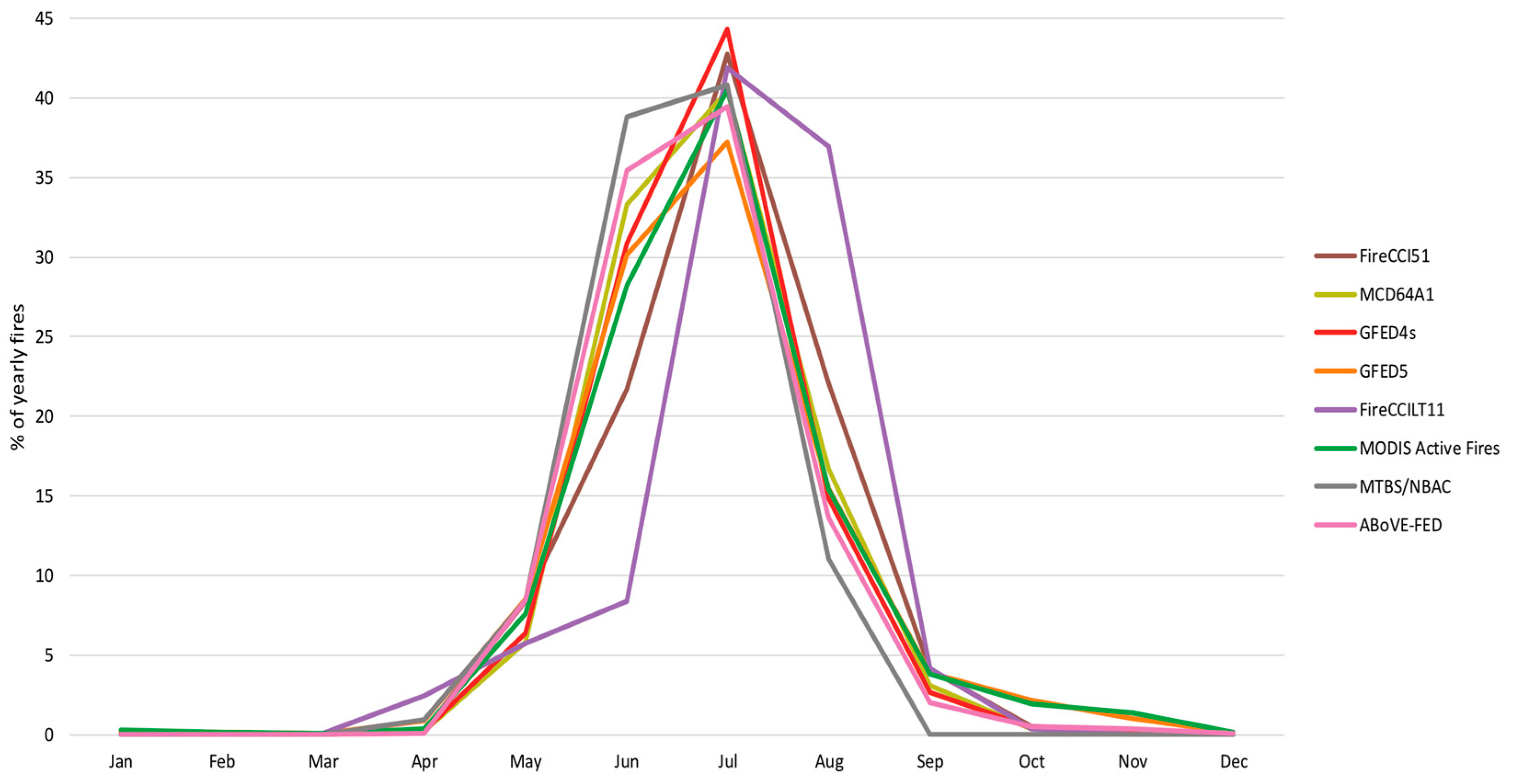
2.3.2. Monthly Fire Percentage
3. Results
3.1. North America
3.2. Central/Northern Siberia
3.3. Southern Siberia
4. Discussion
4.1. Seasonal Patterns
4.2. Advantages and Limitations of Different Methodologies
4.3. Advantages and Limitations of Each BA Product
4.4. Study Limitations
4.5. Comparisons with Previous Literature
5. Conclusions
Supplementary Materials
Author Contributions
Funding
Data Availability Statement
Acknowledgments
Conflicts of Interest
Appendix A
Appendix B
References
- Gauthier, S.; Bernier, P.; Kuuluvainen, T.; Shvidenko, A.Z.; Schepaschenko, D.G. Boreal forest health and global change. Science 2015, 349, 819–822. [Google Scholar] [CrossRef] [PubMed]
- Ruckstuhl, K.E.; Johnson, E.A.; Miyanishi, K. Introduction. Boreal For. Glob. Change 2008, 363, 2243–2247. [Google Scholar]
- Brandt, J.P.; Flannigan, M.D.; Maynard, D.G.; Thompson, I.D.; Volney, W.J.A. An introduction to Canada’s boreal zone: Ecosystem processes, health, sustainability, and environmental issues. Environ. Rev. 2013, 21, 207–226. [Google Scholar] [CrossRef]
- Scheffer, M.; Hirota, M.; Holmgren, M.; Van Nes, E.H.; Chapin, F.S. Thresholds for boreal biome transitions. Proc. Natl. Acad. Sci. USA 2012, 109, 21384–21389. [Google Scholar] [CrossRef] [PubMed]
- Elmendorf, S.C.; Henry, G.H.R.; Hollister, R.D.; Björk, R.G.; Bjorkman, A.D.; Callaghan, T.V.; Collier, L.S.; Cooper, E.J.; Cornelissen, J.H.C.; Day, T.A.; et al. Global assessment of experimental climate warming on tundra vegetation: Heterogeneity over space and time. Ecol. Lett. 2012, 15, 164–175. [Google Scholar] [CrossRef]
- Heijmans, M.M.P.D.; Magnússon, R.Í.; Lara, M.J.; Frost, G.V.; Myers-Smith, I.H.; van Huissteden, J.; Jorgenson, M.T.; Fedorov, A.N.; Epstein, H.E.; Lawrence, D.M.; et al. Tundra vegetation change and impacts on permafrost. Nat. Rev. Earth Environ. 2022, 3, 68–84. [Google Scholar] [CrossRef]
- Chytrý, M.; Horsák, M.; Danihelka, J.; Ermakov, N.; German, D.A.; Hájek, M.; Hájková, P.; Kočí, M.; Kubešová, S.; Lustyk, P.; et al. A modern analogue of the Pleistocene steppe-tundra ecosystem in southern Siberia. Boreas 2019, 48, 36–56. [Google Scholar] [CrossRef]
- Chen, J.; Shao, C.; Jiang, S.; Qu, L.; Zhao, F.; Dong, G. Effects of changes in precipitation on energy and water balance in a Eurasian meadow steppe. Ecol. Process. 2019, 8, 17. [Google Scholar] [CrossRef]
- Miles, M.W.; Miles, V.V.; Esau, I. Varying climate response across the tundra, forest-tundra and boreal forest biomes in northern West Siberia. Environ. Res. Lett. 2019, 14, 075008. [Google Scholar] [CrossRef]
- Chylek, P.; Folland, C.; Klett, J.D.; Wang, M.; Hengartner, N.; Lesins, G.; Dubey, M.K. Annual Mean Arctic Amplification 1970–2020: Observed and Simulated by CMIP6 Climate Models. Geophys. Res. Lett. 2022, 49, e2022GL099371. [Google Scholar] [CrossRef]
- Rantanen, M.; Karpechko, A.Y.; Lipponen, A.; Nordling, K.; Hyvärinen, O.; Ruosteenoja, K.; Vihma, T.; Laaksonen, A. The Arctic has warmed nearly four times faster than the globe since 1979. Commun. Earth Environ. 2022, 3, 168. [Google Scholar] [CrossRef]
- Callaghan, T.V.; Shaduyko, O.; Kirpotin, S.N.; Gordov, E.P. Siberian environmental change: Synthesis of recent studies and opportunities for networking. Ambio 2021, 50, 2104–2127. [Google Scholar] [CrossRef] [PubMed]
- Descals, A.; Gaveau, D.L.A.; Verger, A.; Sheil, D.; Naito, D.; Peñuelas, J. Unprecedented fire activity above the Arctic Circle linked to rising temperatures. Science 2022, 378, 532–537. [Google Scholar] [CrossRef] [PubMed]
- Scholten, R.C.; Coumou, D.; Luo, F.; Veraverbeke, S. Early snowmelt and polar jet dynamics co-influence recent extreme Siberian fire seasons. Science 2022, 378, 1005–1009. [Google Scholar] [CrossRef]
- Turetsky, M.R.; Kane, E.S.; Harden, J.W.; Ottmar, R.D.; Manies, K.L.; Hoy, E.E.; Kasischke, E.S. Recent acceleration of biomass burning and carbon losses in Alaskan forests and peatlands. Nat. Geosci. 2011, 4, 27–31. [Google Scholar] [CrossRef]
- Hanes, C.C.; Wang, X.; Jain, P.; Parisien, M.-A.; Little, J.M.; Flannigan, M.D. Fire-regime changes in Canada over the last half century. Can. J. For. Res. 2019, 49, 256–269. [Google Scholar] [CrossRef]
- Randerson, J.T.; Liu, H.; Flanner, M.G.; Chambers, S.D.; Jin, Y.; Hess, P.G.; Pfister, G.; Mack, M.C.; Treseder, K.K.; Welp, L.R.; et al. The Impact of Boreal Forest Fire on Climate Warming. Science 2006, 314, 1130–1132. [Google Scholar] [CrossRef]
- Olsson, R. Boreal Forest and Climate Change; Air Pollution and Climate Series; Air Pollution & Climate Secretariat & Taiga Rescue Network: Goteborg, Sweden, 2009; Volume 23, p. 32. [Google Scholar]
- Oris, F.; Asselin, H.; Ali, A.A.; Finsinger, W.; Bergeron, Y. Effect of increased fire activity on global warming in the boreal forest. Environ. Rev. 2014, 22, 206–219. [Google Scholar] [CrossRef]
- Potter, S.; Solvik, K.; Erb, A.; Goetz, S.J.; Johnstone, J.F.; Mack, M.C.; Randerson, J.T.; Román, M.O.; Schaaf, C.L.; Turetsky, M.R.; et al. Climate change decreases the cooling effect from postfire albedo in boreal North America. Glob. Chang. Biol. 2020, 26, 1592–1607. [Google Scholar] [CrossRef]
- Phillips, C.A.; Rogers, B.M.; Elder, M.; Cooperdock, S.; Moubarak, M.; Randerson, J.T.; Frumhoff, P.C. Escalating carbon emissions from North American boreal forest wildfires and the climate mitigation potential of fire management. Sci. Adv. 2022, 8, eabl7161. [Google Scholar] [CrossRef]
- Rowe, J.S.; Scotter, G.W. Fire in the boreal forest. Quat. Res. 1973, 3, 444–464. [Google Scholar] [CrossRef]
- Payette, S. Fire as a controlling process in the North American boreal forest. In A Systems Analysis of the Global Boreal Forest; Cambridge University Press: Cambridge, UK, 1992; pp. 144–169. [Google Scholar]
- Stocks, B.J.; Mason, J.A.; Todd, J.B.; Bosch, E.M.; Wotton, B.M.; Amiro, B.D.; Flannigan, M.D.; Hirsch, K.G.; Logan, K.A.; Martell, D.L.; et al. Large forest fires in Canada, 1959–1997. J. Geophys. Res. Atmos. 2002, 107, FFR 5-1–FFR 5-12. [Google Scholar] [CrossRef]
- Baltzer, J.L.; Day, N.J.; Walker, X.J.; Greene, D.; Mack, M.C.; Alexander, H.D.; Arseneault, D.; Barnes, J.; Bergeron, Y.; Boucher, Y.; et al. Increasing fire and the decline of fire adapted black spruce in the boreal forest. Proc. Natl. Acad. Sci. USA 2021, 118, e2024872118. [Google Scholar] [CrossRef] [PubMed]
- Lavoie, L.; Sirois, L. Vegetation changes caused by recent fires in the northern boreal forest of eastern Canada. J. Veg. Sci. 1998, 9, 483–492. [Google Scholar] [CrossRef]
- Shive, K.L.; Preisler, H.K.; Welch, K.R.; Safford, H.D.; Butz, R.J.; O’Hara, K.L.; Stephens, S.L. From the stand scale to the landscape scale: Predicting the spatial patterns of forest regeneration after disturbance. Ecol. Appl. 2018, 28, 1626–1639. [Google Scholar] [CrossRef]
- Johnstone, J.F.; Allen, C.D.; Franklin, J.F.; Frelich, L.E.; Harvey, B.J.; Higuera, P.E.; Mack, M.C.; Meentemeyer, R.K.; Metz, M.R.; Perry, G.L.W.; et al. Changing disturbance regimes, ecological memory, and forest resilience. Front. Ecol. Environ. 2016, 14, 369–378. [Google Scholar] [CrossRef]
- Sun, Q.; Burrell, A.L.; Barrett, K.; Kukavskaya, E.A.; Buryak, L.V.; Kaduk, J.; Baxter, R. Climate Variability May Delay Post-Fire Recovery of Boreal Forest in Southern Siberia, Russia. Remote Sens. 2021, 13, 2247. [Google Scholar] [CrossRef]
- Alfaro-Sánchez, R.; Johnstone, J.F.; Baltzer, J.L. Low-severity fires in the boreal region: Reproductive implications for black spruce stands in between stand-replacing fire events. Ann. Bot. 2024. Online ahead of print. [Google Scholar] [CrossRef]
- Cascio, W.E. Wildland fire smoke and human health. Sci. Total Environ. 2018, 624, 586–595. [Google Scholar] [CrossRef]
- Kayes, I.; Mallik, A. Boreal forests: Distributions, biodiversity, and management. In Life on Land; Springer: Cham, Switzerland, 2020; pp. 1–12. [Google Scholar]
- Li, X.-Y.; Jin, H.-J.; Wang, H.-W.; Marchenko, S.S.; Shan, W.; Luo, D.-L.; He, R.-X.; Spektor, V.; Huang, Y.-D.; Li, X.-Y.; et al. Influences of forest fires on the permafrost environment: A review. Adv. Clim. Chang. Res. 2021, 12, 48–65. [Google Scholar] [CrossRef]
- Balch, J.K.; Bradley, B.A.; Abatzoglou, J.T.; Nagy, R.C.; Fusco, E.J.; Mahood, A.L. Human-started wildfires expand the fire niche across the United States. Proc. Natl. Acad. Sci. USA 2017, 114, 2946–2951. [Google Scholar] [CrossRef] [PubMed]
- Pausas, J.G.; Keeley, J.E. Wildfires and global change. Front. Ecol. Environ. 2021, 19, 387–395. [Google Scholar] [CrossRef]
- Veraverbeke, S.; Rogers, B.M.; Goulden, M.L.; Jandt, R.R.; Miller, C.E.; Wiggins, E.B.; Randerson, J.T. Lightning as a major driver of recent large fire years in North American boreal forests. Nat. Clim. Chang. 2017, 7, 529–534. [Google Scholar] [CrossRef]
- Kharyutkina, E.; Pustovalov, K.; Moraru, E.; Nechepurenko, O. Analysis of Spatio-Temporal Variability of Lightning Activity and Wildfires in Western Siberia during 2016–2021. Atmosphere 2022, 13, 669. [Google Scholar] [CrossRef]
- Xu, W.; Scholten, R.C.; Hessilt, T.D.; Liu, Y.; Veraverbeke, S. Overwintering fires rising in eastern Siberia. Environ. Res. Lett. 2022, 17, 045005. [Google Scholar] [CrossRef]
- McCarty, J.L.; Smith, T.E.L.; Turetsky, M.R. Arctic fires re-emerging. Nat. Geosci. 2020, 13, 658–660. [Google Scholar] [CrossRef]
- Erdős, L.; Török, P.; Veldman, J.W.; Bátori, Z.; Bede-Fazekas, Á.; Magnes, M.; Kröel-Dulay, G.; Tölgyesi, C. How climate, topography, soils, herbivores, and fire control forest–grassland coexistence in the Eurasian forest-steppe. Biol. Rev. 2022, 97, 2195–2208. [Google Scholar] [CrossRef]
- Irannezhad, M.; Liu, J.; Ahmadi, B.; Chen, D. The dangers of Arctic zombie wildfires. Science 2020, 369, 1171. [Google Scholar] [CrossRef]
- de Groot, W.J.; Cantin, A.S.; Flannigan, M.D.; Soja, A.J.; Gowman, L.M.; Newbery, A. A comparison of Canadian and Russian boreal forest fire regimes. For. Ecol. Manag. 2013, 294, 23–34. [Google Scholar] [CrossRef]
- Kharuk, V.I.; Ponomarev, E.I.; Ivanova, G.A.; Dvinskaya, M.L.; Coogan, S.C.P.; Flannigan, M.D. Wildfires in the Siberian taiga. Ambio 2021, 50, 1953–1974. [Google Scholar] [CrossRef]
- Angers, V.; Gauthier, S.; Drapeau, P.; Jayen, K.; Bergeron, Y. Tree mortality and snag dynamics in North American boreal tree species after a wildfire: A long-term study. Int. J. Wildland Fire 2011, 20, 751–763. [Google Scholar] [CrossRef]
- Conard, S.G.; Ivanova, G.A. Wildfire in Russian Boreal Forests—Potential Impacts of Fire Regime Characteristics on Emissions and Global Carbon Balance Estimates. Environ. Pollut. 1997, 98, 305–313. [Google Scholar] [CrossRef]
- Shvetsov, E.G.; Kukavskaya, E.A.; Buryak, L.V.; Barrett, K. Assessment of post-fire vegetation recovery in Southern Siberia using remote sensing observations. Environ. Res. Lett. 2019, 14, 055001. [Google Scholar] [CrossRef]
- Shvetsov, E.G.; Golyukov, A.S.; Kharuk, V.I. Long-Term Dynamics of Forest Fires in Southern Siberia. Contemp. Probl. Ecol. 2023, 16, 205–216. [Google Scholar] [CrossRef]
- Zhang, J.-H.; Yao, F.-M.; Liu, C.; Yang, L.-M.; Boken, V.K. Detection, Emission Estimation and Risk Prediction of Forest Fires in China Using Satellite Sensors and Simulation Models in the Past Three Decades—An Overview. Int. J. Environ. Res. Public Health 2011, 8, 3156–3178. [Google Scholar] [CrossRef] [PubMed]
- Ulbricht, K.A.; Heckendorff, W.D. Satellite images for recognition of landscape and landuse changes. ISPRS J. Photogramm. Remote Sens. 1998, 53, 235–243. [Google Scholar] [CrossRef]
- Cheng, K.S.; Wei, C.; Chang, S.C. Locating landslides using multi-temporal satellite images. Adv. Space Res. 2004, 33, 296–301. [Google Scholar] [CrossRef]
- Skakun, S.; Kussul, N.; Shelestov, A.; Kussul, O. Flood Hazard and Flood Risk Assessment Using a Time Series of Satellite Images: A Case Study in Namibia. Risk Anal. 2014, 34, 1521–1537. [Google Scholar] [CrossRef]
- Tang, H.; Li, Z.-L. Applications of Thermal Remote Sensing in Agriculture Drought Monitoring and Thermal Anomaly Detection. In Quantitative Remote Sensing in Thermal Infrared: Theory and Applications; Springer: Berlin/Heidelberg, Germany, 2014; pp. 203–256. [Google Scholar]
- Dao, M.; Kwan, C.; Ayhan, B.; Tran, T.D. Burn scar detection using cloudy MODIS images via low-rank and sparsity-based models. In Proceedings of the 2016 IEEE Global Conference on Signal and Information Processing (GlobalSIP), Washington, DC, USA, 7–9 December 2016; pp. 177–181. [Google Scholar]
- Roteta, E.; Bastarrika, A.; Ibisate, A.; Chuvieco, E. A Preliminary Global Automatic Burned-Area Algorithm at Medium Resolution in Google Earth Engine. Remote Sens. 2021, 13, 4298. [Google Scholar] [CrossRef]
- Dutra, D.J.; Fearnside, P.M.; Yanai, A.M.; Graça, P.M.L.d.A.; Dalagnol, R.; Pessôa, A.C.M.; Cabral, B.F.; Burton, C.; Jones, C.; Betts, R.A. Burned area mapping in Different Data Products for the Southwest of the Brazilian Amazon. Rev. Bras. Cartogr. 2023, 75, 1–16. [Google Scholar] [CrossRef]
- Fornacca, D.; Ren, G.; Xiao, W. Performance of Three MODIS Fire Products (MCD45A1, MCD64A1, MCD14ML), and ESA Fire_CCI in a Mountainous Area of Northwest Yunnan, China, Characterized by Frequent Small Fires. Remote Sens. 2017, 9, 1131. [Google Scholar] [CrossRef]
- Humber, M.L.; Boschetti, L.; Giglio, L.; Justice, C.O. Spatial and temporal intercomparison of four global burned area products. Int. J. Digit. Earth 2019, 12, 460–484. [Google Scholar] [CrossRef]
- Pessôa, A.C.M.; Anderson, L.O.; Carvalho, N.S.; Campanharo, W.A.; Junior, C.H.L.S.; Rosan, T.M.; Reis, J.B.C.; Pereira, F.R.S.; Assis, M.; Jacon, A.D.; et al. Intercomparison of Burned Area Products and Its Implication for Carbon Emission Estimations in the Amazon. Remote Sens. 2020, 12, 3864. [Google Scholar] [CrossRef]
- Turco, M.; Herrera, S.; Tourigny, E.; Chuvieco, E.; Provenzale, A. A comparison of remotely-sensed and inventory datasets for burned area in Mediterranean Europe. Int. J. Appl. Earth Obs. Geoinf. 2019, 82, 101887. [Google Scholar] [CrossRef]
- Valencia, G.M.; Anaya, J.A.; Velásquez, É.A.; Ramo, R.; Caro-Lopera, F.J. About Validation-Comparison of Burned Area Products. Remote Sens. 2020, 12, 3972. [Google Scholar] [CrossRef]
- Zhang, T.; Wooster, M.J.; De Jong, M.C.; Xu, W. How Well Does the ‘Small Fire Boost’ Methodology Used within the GFED4.1s Fire Emissions Database Represent the Timing, Location and Magnitude of Agricultural Burning? Remote Sens. 2018, 10, 823. [Google Scholar] [CrossRef]
- Olson, D.M.; Dinerstein, E.; Wikramanayake, E.D.; Burgess, N.D.; Powell, G.V.N.; Underwood, E.C.; D’amico, J.A.; Itoua, I.; Strand, H.E.; Morrison, J.C.; et al. Terrestrial Ecoregions of the World: A New Map of Life on Earth: A new global map of terrestrial ecoregions provides an innovative tool for conserving biodiversity. BioScience 2001, 51, 933–938. [Google Scholar] [CrossRef]
- Talucci, A.C.; Loranty, M.M.; Alexander, H.D. Siberian taiga and tundra fire regimes from 2001–2020. Environ. Res. Lett. 2022, 17, 025001. [Google Scholar] [CrossRef]
- Soja, A.J.; Sukhinin, A.I.; Cahoon, D.R., Jr.; Shugart, H.H.; Stackhouse, P.W., Jr. AVHRR-derived fire frequency, distribution and area burned in Siberia. Int. J. Remote Sens. 2004, 25, 1939–1960. [Google Scholar] [CrossRef]
- Rogers, B.M.; Soja, A.J.; Goulden, M.L.; Randerson, J.T. Influence of tree species on continental differences in boreal fires and climate feedbacks. Nat. Geosci. 2015, 8, 228–234. [Google Scholar] [CrossRef]
- Rogers, B.M.; Soja, A.J.; Goulden, M.L.; Randerson, J.T. Fire Intensity and Burn Severity Metrics for Circumpolar Boreal Forests, 2001–2013; ORNL Distributed Active Archive Center: Oak Ridge, TN, USA, 2017. [Google Scholar] [CrossRef]
- Brassard, B.W.; Chen, H.Y.H. Stand Structural Dynamics of North American Boreal Forests. Crit. Rev. Plant Sci. 2006, 25, 115–137. [Google Scholar] [CrossRef]
- Friedl, M.A.; Sulla-Menashe, D. MODIS/Terra+Aqua Land Cover Type Yearly L3 Global 500m SIN Grid V061, N.E.L.P.D.A.A. Center, Editor. 2022. Available online: https://lpdaac.usgs.gov/products/mcd12q1v061/ (accessed on 20 February 2024).
- Hart, S.A.; Chen, H.Y.H. Understory Vegetation Dynamics of North American Boreal Forests. Crit. Rev. Plant Sci. 2006, 25, 381–397. [Google Scholar] [CrossRef]
- Lizundia-Loiola, J.; Otón, G.; Ramo, R.; Chuvieco, E. A spatio-temporal active-fire clustering approach for global burned area mapping at 250 m from MODIS data. Remote Sens. Environ. 2020, 236, 111493. [Google Scholar] [CrossRef]
- Giglio, L.; Boschetti, L.; Roy, D.P.; Humber, M.L.; Justice, C.O. The Collection 6 MODIS burned area mapping algorithm and product. Remote Sens. Environ. 2018, 217, 72–85. [Google Scholar] [CrossRef]
- Long, T.; Zhang, Z.; He, G.; Jiao, W.; Tang, C.; Wu, B.; Zhang, X.; Wang, G.; Yin, R. 30 m Resolution Global Annual Burned Area Mapping Based on Landsat Images and Google Earth Engine. Remote Sens. 2019, 11, 489. [Google Scholar] [CrossRef]
- Giglio, L.; Randerson, J.T.; Van Der Werf, G.R. Analysis of daily, monthly, and annual burned area using the fourth-generation global fire emissions database (GFED4). J. Geophys. Res. Biogeosci. 2013, 118, 317–328. [Google Scholar] [CrossRef]
- van der Werf, G.R.; Randerson, J.T.; Giglio, L.; van Leeuwen, T.T.; Chen, Y.; Rogers, B.M.; Mu, M.; van Marle, M.J.E.; Morton, D.C.; Collatz, G.J.; et al. Global fire emissions estimates during 1997–2016. Earth Syst. Sci. Data 2017, 9, 697–720. [Google Scholar] [CrossRef]
- Chen, Y.; Hall, J.; van Wees, D.; Andela, N.; Hantson, S.; Giglio, L.; van der Werf, G.R.; Morton, D.C.; Randerson, J.T. Multi-decadal trends and variability in burned area from the fifth version of the Global Fire Emissions Database (GFED5). Earth Syst. Sci. Data 2023, 15, 5227–5259. [Google Scholar] [CrossRef]
- Otón, G.; Lizundia-Loiola, J.; Pettinari, M.L.; Chuvieco, E. Development of a consistent global long-term burned area product (1982–2018) based on AVHRR-LTDR data. Int. J. Appl. Earth Obs. Geoinf. 2021, 103, 102473. [Google Scholar] [CrossRef]
- Eidenshink, J.; Schwind, B.; Brewer, K.; Zhu, Z.-L.; Quayle, B.; Howard, S. A Project for Monitoring Trends in Burn Severity. Fire Ecol. 2007, 3, 3–21. [Google Scholar] [CrossRef]
- Hall, R.J.; Skakun, R.S.; Metsaranta, J.M.; Landry, R.; Fraser, R.H.; Raymond, D.; Gartrell, M.; Decker, V.; Little, J. Generating annual estimates of forest fire disturbance in Canada: The National Burned Area Composite. Int. J. Wildland Fire 2020, 29, 878–891. [Google Scholar] [CrossRef]
- Skakun, R.S.; Castilla, G.; Metsaranta, J.M.; Whitman, E.; Rodrigue, S.; Little, J.; Groenewegen, K.; Coyle, M. Extending the National Burned Area Composite Time Series of Wildfires in Canada. Remote Sens. 2022, 14, 3050. [Google Scholar] [CrossRef]
- Potter, S.; Cooperdock, S.; Veraverbeke, S.; Walker, X.; Mack, M.C.; Goetz, S.J.; Baltzer, J.L.; Bourgeau-Chavez, L.; Burrell, A.; Dieleman, C.; et al. Burned area and carbon emissions across northwestern boreal North America from 2001–2019. Biogeosciences 2023, 20, 2785–2804. [Google Scholar] [CrossRef]
- Bartalev, S.A.; Egorov, V.I.; Efremov, V.S.; Flitman, E.V.; Loupian, E.A.; Stytsenko, F.V. Assessment of burned forest areas over the Russian federation from MODIS and Landsat-TM/ETM+ imagery. In Global Forest Monitoring from Earth Observation; CRC Press: Boca Raton, FL, USA, 2012; pp. 245–271. [Google Scholar]
- Loboda, T.V.; Hall, J.V.; Chen, D.; Hoffman-Hall, A.; Shevade, V.S.; Argueta, F.; Liang, X. Arctic Boreal Annual Burned Area, Circumpolar Boreal Forest and Tundra, V2, 2002–2022; ORNL Distributed Active Archive Center: Oak Ridge, TN, USA, 2024. [Google Scholar] [CrossRef]
- Giglio, L.; Schroeder, W.; Justice, C.O. The collection 6 MODIS active fire detection algorithm and fire products. Remote Sens. Environ. 2016, 178, 31–41. [Google Scholar] [CrossRef] [PubMed]
- Chuvieco, E.; Yue, C.; Heil, A.; Mouillot, F.; Alonso-Canas, I.; Padilla, M.; Pereira, J.M.; Oom, D.; Tansey, K. A new global burned area product for climate assessment of fire impacts. Glob. Ecol. Biogeogr. 2016, 25, 619–629. [Google Scholar] [CrossRef]
- Chuvieco, E.; Lizundia-Loiola, J.; Pettinari, M.L.; Ramo, R.; Padilla, M.; Tansey, K.; Mouillot, F.; Laurent, P.; Storm, T.; Heil, A.; et al. Generation and analysis of a new global burned area product based on MODIS 250 m reflectance bands and thermal anomalies. Earth Syst. Sci. Data 2018, 10, 2015–2031. [Google Scholar] [CrossRef]
- Vermote, E.F.; Kotchenova, S.Y.; Ray, J.P. MODIS Surface Reflectance User’s Guide; MODIS Land Surface Reflectance Science Computing Facility: Greenbelt, MD, USA, 2011; Volume 1, pp. 1–40. [Google Scholar]
- ESA. Land Cover CCI Product User Guide Version 2; ESA: Harwell, UK, 2017. [Google Scholar]
- Vermote, E.F.; El Saleous, N.Z.; Justice, C.O. Atmospheric correction of MODIS data in the visible to middle infrared: First results. Remote Sens. Environ. 2002, 83, 97–111. [Google Scholar] [CrossRef]
- Justice, C.O.; Giglio, L.; Korontzi, S.; Owens, J.; Morisette, J.T.; Roy, D.; Descloitres, J.; Alleaume, S.; Petitcolin, F.; Kaufman, Y. The MODIS fire products. Remote Sens. Environ. 2002, 83, 244–262. [Google Scholar] [CrossRef]
- Friedl, M.A.; Sulla-Menashe, D.; Tan, B.; Schneider, A.; Ramankutty, N.; Sibley, A.; Huang, X. MODIS Collection 5 global land cover: Algorithm refinements and characterization of new datasets. Remote Sens. Environ. 2010, 114, 168–182. [Google Scholar] [CrossRef]
- Friedl, M.A.; Sulla-Menashe, D. MODIS/Terra+Aqua Land Cover Type Yearly L3 Global 0.05Deg CMG V006; NASA EOSDIS Land Processes Distributed Active Archive Center: Sioux Falls, SD, USA, 2015. [Google Scholar] [CrossRef]
- Randerson, J.T.; Chen, Y.; van der Werf, G.R.; Rogers, B.M.; Morton, D.C. Global burned area and biomass burning emissions from small fires. J. Geophys. Res. Biogeosci. 2012, 117. [Google Scholar] [CrossRef]
- Sulla-Menashe, D.; Friedl, M.A. User Guide to Collection 6 MODIS Land Cover (MCD12Q1 and MCD12C1) Product; Usgs: Reston, VA, USA, 2018; Volume 1, p. 18.
- DiMiceli, C.; Carroll, M.; Sohlberg, R.; Kim, D.; Kelly, M.; Townshend, J. MOD44B MODIS/Terra Vegetation Continuous Fields Yearly L3 Global 250 m SIN Grid V006; NASA EOSDIS Land Processes Distributed Active Archive Center: Sioux Falls, SD, USA, 2015. [Google Scholar] [CrossRef]
- Copernicus. Copernicus. Algorithm Theoretical Basis Document, Version 1.0. D1.5.2-v.1.0_ATBD_ICDR_LC_v2.1_PRODUCTS_v1.0.1; UCLouvain: Louvain, Belgium, 2019; p. 62. [Google Scholar]
- Fraser, R.H.; Li, Z.; Cihlar, J. Hotspot and NDVI Differencing Synergy (HANDS): A New Technique for Burned Area Mapping over Boreal Forest. Remote Sens. Environ. 2000, 74, 362–376. [Google Scholar] [CrossRef]
- Fraser, R.H.; Hall, R.J.; Landry, R.; Lynham, T.; Raymond, D.; Lee, B.; Li, Z. Validation and Calibration of Canada-Wide Coarse-Resolution Satellite Burned-Area Maps. Photogramm. Eng. Remote Sens. 2004, 4, 451–460. [Google Scholar] [CrossRef]
- Fernandes, R.; Leblanc, S.G. Parametric (modified least squares) and non-parametric (Theil–Sen) linear regressions for predicting biophysical parameters in the presence of measurement errors. Remote Sens. Environ. 2005, 95, 303–316. [Google Scholar] [CrossRef]
- Natural Resources Canada, Canadian National Fire Database; Natural Resources Canada, Canadian Forest Service, Northern Forestry Centre: Edmonton, AB, Canada, 2022.
- Kolden, C.A.; Weisberg, P.J. Assessing Accuracy of Manually-mapped Wildfire Perimeters in Topographically Dissected Areas. Fire Ecol. 2007, 3, 22–31. [Google Scholar] [CrossRef]
- Hermosilla, T.; Wulder, M.A.; White, J.C.; Coops, N.C.; Hobart, G.W.; Campbell, L.B. Mass data processing of time series Landsat imagery: Pixels to data products for forest monitoring. Int. J. Digit. Earth 2016, 9, 1035–1054. [Google Scholar] [CrossRef]
- Pekel, J.-F.; Cottam, A.; Gorelick, N.; Belward, A.S. High-resolution mapping of global surface water and its long-term changes. Nature 2016, 540, 418–422. [Google Scholar] [CrossRef]
- Latifovic, R.; Homer, C.; Ressl, R.; Pouliot, D.A.; Hossian, S.; Colditz, R.; Olthof, I.; Chandra, G.; Victoria, A. North American Land Change Monitoring System. In Remote Sensing of Land Use and Land Cover: Principles and Applications; CRC Press: Boca Raton, FL, USA, 2012; pp. 303–324. [Google Scholar]
- Hermosilla, T.; Wulder, M.A.; White, J.C.; Coops, N.C.; Hobart, G.W. An integrated Landsat time series protocol for change detection and generation of annual gap-free surface reflectance composites. Remote Sens. Environ. 2015, 158, 220–234. [Google Scholar] [CrossRef]
- Vermote, E.F. MOD09A1 MODIS/Terra Surface Reflectance 8-Day L3 Global 500 m SIN Grid V006; NASA EOSDIS Land Processes Distributed Active Archive Center: Sioux Falls, SD, USA, 2015. [Google Scholar] [CrossRef]
- Carroll, M.; DiMiceli, C.; Townshend, J.; Sohlberg, R.; Hubbard, A.B.; Wooten, M.R. A new global raster water mask at 250 m resolution. Int. J. Digit. Earth 2009, 2, 291–308. [Google Scholar] [CrossRef]
- Hansen, M.C.; DeFries, R.S.; Townshend, J.; Carroll, M.; DiMiceli, C.; Sohlberg, R. Global percent tree cover at a spatial resolution of 500 meters: First results of the MODIS vegetation continuous fields algorithm. Earth Interact. 2003, 7, 1–15. [Google Scholar] [CrossRef]
- Giglio, L.; van der Werf, G.R.; Randerson, J.T.; Collatz, G.J.; Kasibhatla, P. Global estimation of burned area using MODIS active fire observations. Atmos. Chem. Phys. 2006, 6, 957–974. [Google Scholar] [CrossRef]
- Hantson, S.; Padilla, M.; Corti, D.; Chuvieco, E. Strengths and weaknesses of MODIS hotspots to characterize global fire occurrence. Remote Sens. Environ. 2013, 131, 152–159. [Google Scholar] [CrossRef]
- Google. ee.Reducer.sum. 13 July 2024. Available online: https://developers.google.com/earth-engine/apidocs/ee-reducer-sum (accessed on 9 August 2024).
- Gorelick, N.; Hancher, M.; Dixon, M.; Ilyushchenko, S.; Thau, D.; Moore, R. Google Earth Engine: Planetary-scale geospatial analysis for everyone. Remote Sens. Environ. 2017, 202, 18–27. [Google Scholar] [CrossRef]
- Burrell, A.L.; Sun, Q.; Baxter, R.; Kukavskaya, E.A.; Zhila, S.V.; Shestakova, T.; Rogers, B.M.; Kaduk, J.; Barrett, K. Climate change, fire return intervals and the growing risk of permanent forest loss in boreal Eurasia. Sci. Total Environ. 2022, 831, 154885. [Google Scholar] [CrossRef]
- Google. ee.Reducer.frequencyHistogram. 13 July 2024. Available online: https://developers.google.com/earth-engine/apidocs/ee-reducer-frequencyhistogram (accessed on 9 August 2024).
- Liu, T.; Marlier, M.; Karambelas, A.; Jain, M.; Singh, S.; Singh, M.; Gautam, R.; DeFries, R.S. Missing emissions from post-monsoon agricultural fires in northwestern India: Regional limitations of MODIS burned area and active fire products. Environ. Res. Commun. 2019, 1, 011007. [Google Scholar] [CrossRef]
- Yao, Q.; Fang, K.; Ou, T.; Zhou, F.; He, M.; Zheng, B.; Liu, J.; Xing, H.; Trouet, V. Reply to: Fire activity as measured by burned area reveals weak effects of ENSO in China. Nat. Commun. 2022, 13, 4317. [Google Scholar] [CrossRef]
- Hawbaker, T.J.; Radeloff, V.C.; Syphard, A.D.; Zhu, Z.; Stewart, S.I. Detection rates of the MODIS active fire product in the United States. Remote Sens. Environ. 2008, 112, 2656–2664. [Google Scholar] [CrossRef]
- Flannigan, M.D.; Stocks, B.; Turetsky, M.; Wotton, M. Impacts of climate change on fire activity and fire management in the circumboreal forest. Glob. Chang. Biol. 2009, 15, 549–560. [Google Scholar] [CrossRef]
- Nefedova, T. The 2010 Catastrophic Forest Fires in Russia: Consequence of Rural Depopulation? In The Demography of Disasters: Impacts for Population and Place; Springer: Cham, Switzerland, 2021; pp. 71–79. [Google Scholar]
- Shvidenko, A.Z.; Schepaschenko, D.G.; Sukhinin, A.; McCallum, I.; Maksyutov, S. Carbon emissions from forest fires in boreal Eurasia between 1998–2010. In Proceedings of the 5th International Wildland Fire Conference, Sun City, South Africa, 9–13 May 2011. [Google Scholar]
- Shvidenko, A.Z.; Schepaschenko, D.G. Climate Change and Wildfires in Russia. Contemp. Probl. Ecol. 2013, 6, 683–692. [Google Scholar] [CrossRef]
- Romanov, A.A.; Tamarovskaya, A.N.; Gloor, E.; Brienen, R.; Gusev, B.A.; Leonenko, E.V.; Vasiliev, A.S.; Krikunov, E.E. Reassessment of carbon emissions from fires and a new estimate of net carbon uptake in Russian forests in 2001–2021. Sci. Total Environ. 2022, 846, 157322. [Google Scholar] [CrossRef]
- Chan, A.H.Y.; Guizar-Coutiño, A.; Kalamandeen, M.; Coomes, D.A. Reconstructing 34 Years of Fire History in the Wet, Subtropical Vegetation of Hong Kong Using Landsat. Remote Sens. 2023, 15, 1489. [Google Scholar] [CrossRef]
- Storey, J.C.; Scaramuzza, P.L.; Schmidt, G.L. Landsat 7 Scan Line Corrector-Off Gap-Filled Product Development. 2005. Available online: https://www.asprs.org/a/publications/proceedings/pecora16/Storey_J.pdf (accessed on 2 September 2024).
- Roy, D.P.; Boschetti, L.; Justice, C.O.; Ju, J. The collection 5 MODIS burned area product—Global evaluation by comparison with the MODIS active fire product. Remote Sens. Environ. 2008, 112, 3690–3707. [Google Scholar] [CrossRef]
- Moreno-Ruiz, J.-A.; García-Lázaro, J.-R.; Arbelo, M.; Hernández-Leal, P.A. A satellite-based burned area dataset for the northern boreal region from 1982 to 2020. Int. J. Wildland Fire 2023, 32, 854–871. [Google Scholar] [CrossRef]
- Nagol, J.R.; Vermote, E.F.; Prince, S.D. Effects of atmospheric variation on AVHRR NDVI data. Remote Sens. Environ. 2009, 113, 392–397. [Google Scholar] [CrossRef]
- Beck, H.E.; McVicar, T.R.; van Dijk, A.I.J.M.; Schellekens, J.; de Jeu, R.A.M.; Bruijnzeel, L.A. Global evaluation of four AVHRR–NDVI data sets: Intercomparison and assessment against Landsat imagery. Remote Sens. Environ. 2011, 115, 2547–2563. [Google Scholar] [CrossRef]
- Dech, S.; Holzwarth, S.; Asam, S.; Andresen, T.; Bachmann, M.; Boettcher, M.; Dietz, A.; Eisfelder, C.; Frey, C.; Gesell, G.; et al. Potential and Challenges of Harmonizing 40 Years of AVHRR Data: The TIMELINE Experience. Remote Sens. 2021, 13, 3618. [Google Scholar] [CrossRef]
- Zhang, X.; Kondragunta, S.; Quayle, B. Estimation of Biomass Burned Areas Using Multiple-Satellite-Observed Active Fires. IEEE Trans. Geosci. Remote Sens. 2011, 49, 4469–4482. [Google Scholar] [CrossRef]
- Loboda, T.V.; Hoy, E.E.; Giglio, L.; Kasischke, E.S. Mapping burned area in Alaska using MODIS data: A data limitations-driven modification to the regional burned area algorithm. Int. J. Wildland Fire 2011, 20, 487–496. [Google Scholar] [CrossRef]
- Schroeder, W.; Oliva, P.; Giglio, L.; Csiszar, I.A. The New VIIRS 375m active fire detection data product: Algorithm description and initial assessment. Remote Sens. Environ. 2014, 143, 85–96. [Google Scholar] [CrossRef]
- Oliva, P.; Schroeder, W. Assessment of VIIRS 375m active fire detection product for direct burned area mapping. Remote Sens. Environ. 2015, 160, 144–155. [Google Scholar] [CrossRef]
- Boschetti, L.; Sparks, A.; Roy, D.; Giglio, L.; San-Miguel-Ayanz, J. GWIS National and Sub-National Fire Activity Data from the NASA MODIS Collection 6 Burned Area Product in Support of Policy Making, Carbon Inventories and Natural Resource Management; NASA Applied Sciences: New York, NY, USA, 2020. [Google Scholar]
- Alencar, A.A.C.; Arruda, V.L.S.; da Silva, W.V.; Conciani, D.E.; Costa, D.P.; Crusco, N.; Duverger, S.G.; Ferreira, N.C.; Franca-Rocha, W.; Hasenack, H.; et al. Long-Term Landsat-Based Monthly Burned Area Dataset for the Brazilian Biomes Using Deep Learning. Remote Sens. 2022, 14, 2510. [Google Scholar] [CrossRef]
- van der Werf, G.R.; Randerson, J.T.; Giglio, L.; Collatz, G.J.; Kasibhatla, P.S.; Arellano, A.F., Jr. Interannual variability in global biomass burning emissions from 1997 to 2004. Atmos. Chem. Phys. 2006, 6, 3423–3441. [Google Scholar] [CrossRef]
- Lizundia-Loiola, J.; Franquesa, M.; Khairoun, A.; Chuvieco, E. Global burned area mapping from Sentinel-3 Synergy and VIIRS active fires. Remote Sens. Environ. 2022, 282, 113298. [Google Scholar] [CrossRef]


| Title | Reference | Study Area(s) | Products Used | Year(s) of Interest |
|---|---|---|---|---|
| Burned area mapping in Different Data Products for the Southwest of the Brazilian Amazon | Dutra et al. (2023) [55] | Southwestern Brazilian Amazon | MCD64A1 (C6) GABAM GWIS MAPBIOMAS | 2019 |
| Performance of Three MODIS Fire Products (MCD45A1, MCD64A1, MCD14ML), and ESA Fire_CCI in a Mountainous Area of Northwest Yunnan, China, Characterized by Frequent Small Fires | Fornacca et al. (2017) [56] | Northwest Yunnan, China | MCD45A1 (C5.1) MCD64A1 (C6) FireCCI41 MODIS active fires | 2006 and 2009 |
| Spatial and temporal intercomparison of four global burned area products | Humber et al. (2019) [57] | Global | MCD45A1 (C5) MCD64A1 (C6) FireCCI41 Copernicus Burnt Area MODIS active fires | 2005 to 2011 |
| Intercomparison of Burned Area Products and Its Implication for Carbon Emission Estimations in the Amazon | Pessôa et al. (2020) [58] | Brazilian Amazon | MCD64A1 (C6) FireCCI50 GABAM TREES | 2015 |
| A comparison of remotely-sensed and inventory datasets for burned area in Mediterranean Europe | Turco et al. (2019) [59] | Mediterranean Europe | MCD64A1 (C6) FireCCI51 GFED4 GFED4s EFFIS | 2001 to 2011 |
| About Validation-Comparison of Burned Area Products | Valencia et al. (2020) [60] | Northern Hemisphere Africa and South America | MCD45A1 (C5) MCD64A1 (C5) MCD64A1 (C6) FireCCI41 FireCCI50 | 2007 and 2008 |
| How Well Does the ‘Small Fire Boost’ Methodology Used within the GFED4.1s Fire Emissions Database Represent the Timing, Location and Magnitude of Agricultural Burning? | Zhang et al. (2018) [61] | Eastern China and Northwest India | MCD64A1 (C6) GFED4 GFED4s MODIS active fires VIIRS active fires | 2015 to 2016 (Eastern China) 2016 (Northwest India) |
| Long Name | Short Name | Reference | Years | Temporal Resolution | Spatial Resolution | Product Type | Extent | Main Production Methods |
|---|---|---|---|---|---|---|---|---|
| ESA Fire Climate Change Initiative: MODIS Fire_cci Burned Area Pixel product, Version 5.1 | FireCCI51 | Lizundia-Loiola et al. (2020) [70] https://doi.org/10.5285/58f00d8814064b79a0c49662ad3af537 | 2001–present | Monthly | 250 m 0.25° | Pixel Grid | Global | MODIS imagery: min. NIR value around fire found. Hotspot seeds generated and grown. |
| Collection 6 MCD64A1 MODIS Burned Area Monthly Global 500 m | MCD64A1 | Giglio et al. (2018) [71] https://doi.org/10.5067/MODIS/MCD64A1.061 | 2001–present | Monthly | 500 m | Pixel | Global | MODIS imagery: max. VI values around fire found. Probabilistic thresholds determined to classify fires and surrounding cells. |
| 30 m Resolution Global Annual Burned Area Maps | GABAM | Long et al. (2019) [72] https://doi.org/10.7910/DVN/3CTMKP | 1985–2021 | Annual | 30 m | Pixel | Global | Landsat imagery: 6 image bands and 8 spectral indices used. Random forest model, thresholds and iterative procedures used to grow fires. |
| Global Fire Emissions Database, Version 4.1 with small fires | GFED4s | Giglio et al. (2013) [73] van der Werf et al. (2017) [74] https://doi.org/10.3334/ORNLDAAC/1293 | 1997–2016 | Monthly | 0.25° | Grid | Global | Derived from MCD64A1 (C5.1) and combined with MODIS active fire data. dNBR used. |
| Global Fire Emissions Database, Version 5 | GFED5 | Chen et al. (2023) [75] https://doi.org/10.5281/zenodo.7668424 | 1997–2020 | Monthly | 1° (1997–2000) 0.25° (2001–2020) | Grid | Global | Derived from MCD64A1 (C6) and combined with MODIS active fire data. Corrective scalars used to make adjustments. |
| ESA Fire Climate Change Initiative: AVHRR-LTDR Burned Area Pixel product, version 1.1 | FireCCILT11 | Otón et al. (2021) [76] https://dx.doi.org/10.5285/b1bd715112ca43ab948226d11d72b85e | 1982–2018 (excluding 1994) | Monthly | 0.05° 0.25° | Pixel Grid | Global | AVHRR imagery. Random forest models and thresholds used alongside the LTDR burned index. |
| Monitoring Trends in Burn Severity | MTBS | Eidenshink et al. (2007) [77] https://mtbs.gov/direct-download (accessed on 1 October 2023) | 1984–present | Annual | 30 m | Polygon | United States of America | Landsat imagery: dNBR calculated and perimeters delineated. |
| Canadian National Fire Database National Burned Area Composite | NBAC | Hall et al. (2020) [78] Skakun et al. (2022) [79] https://cwfis.cfs.nrcan.gc.ca/datamart/download/nbac (accessed on 1 October 2023) | 1986–present | Annual | 30 m | Polygon | Canada | Landsat imagery: NDVI and dNBR used alongside MODIS active fire data. |
| NASA Arctic–Boreal Vulnerability Experiment Fire Emissions Database | ABoVE-FED | Potter et al. (2023) [80] https://doi.org/10.3334/ORNLDAAC/2063 | 2001–2020 | Annual | 500 m | Pixel | Alaska and Canada | Landsat imagery: dNBR used alongside MODIS active fire data. |
| Surface Reflectance Burned Area product | SRBA | Bartalev et al. (2012) [81] | 2006–2020 | Annual | 250 m | Pixel | Russian Federation | MODIS imagery: dNBR used with thresholds and MODIS active fire data. |
| Fire perimeter product | Talucci et al. | Talucci et al. (2022) [63] https://arcticdata.io/catalog/view/doi%3A10.18739%2FA2GB1XJ4M (accessed on 26 September 2023) | 2001–2020 | Annual | 30 m | Polygon | Siberia | Landsat imagery: dNBR used alongside MODIS active fire data. |
| Arctic Boreal Burned Area Dataset | ABBA | Loboda et al. (2024) [82] https://doi.org/10.3334/ORNLDAAC/2328 | 2002–2022 | Annual | 500 m | Pixel | Boreal and tundra biomes | MODIS imagery: dNBR used alongside MODIS active fire data. |
| MODIS MOD14A1 (Terra) and MYD14A1 (Aqua) Active Fire Data Products Version 6.1 | MODIS active fires | Giglio et al. (2016) [83] https://doi.org/10.5067/MODIS/MOD14A1.061 https://doi.org/10.5067/MODIS/MYD14A1.061 | 2000–present (MOD14A1) 2002–present (MYD14A1) | Daily | 1000 m | Pixel | Global | MODIS imagery: thresholds used and rejection tests conducted. |
Disclaimer/Publisher’s Note: The statements, opinions and data contained in all publications are solely those of the individual author(s) and contributor(s) and not of MDPI and/or the editor(s). MDPI and/or the editor(s) disclaim responsibility for any injury to people or property resulting from any ideas, methods, instructions or products referred to in the content. |
© 2024 by the authors. Licensee MDPI, Basel, Switzerland. This article is an open access article distributed under the terms and conditions of the Creative Commons Attribution (CC BY) license (https://creativecommons.org/licenses/by/4.0/).
Share and Cite
Clelland, A.A.; Marshall, G.J.; Baxter, R.; Potter, S.; Talucci, A.C.; Rady, J.M.; Genet, H.; Rogers, B.M.; Natali, S.M. Annual and Seasonal Patterns of Burned Area Products in Arctic-Boreal North America and Russia for 2001–2020. Remote Sens. 2024, 16, 3306. https://doi.org/10.3390/rs16173306
Clelland AA, Marshall GJ, Baxter R, Potter S, Talucci AC, Rady JM, Genet H, Rogers BM, Natali SM. Annual and Seasonal Patterns of Burned Area Products in Arctic-Boreal North America and Russia for 2001–2020. Remote Sensing. 2024; 16(17):3306. https://doi.org/10.3390/rs16173306
Chicago/Turabian StyleClelland, Andrew A., Gareth J. Marshall, Robert Baxter, Stefano Potter, Anna C. Talucci, Joshua M. Rady, Hélène Genet, Brendan M. Rogers, and Susan M. Natali. 2024. "Annual and Seasonal Patterns of Burned Area Products in Arctic-Boreal North America and Russia for 2001–2020" Remote Sensing 16, no. 17: 3306. https://doi.org/10.3390/rs16173306