Snow Detection in Gaofen-1 Multi-Spectral Images Based on Swin-Transformer and U-Shaped Dual-Branch Encoder Structure Network with Geographic Information

Abstract

Snow detection is imperative in remote sensing for various applications, including climate change monitoring, water resources management, and disaster warning. Recognizing the limitations of current deep learning algorithms in cloud and snow boundary segmentation, as well as issues like detail snow information loss and mountainous snow omission, this paper presents a novel snow detection network based on Swin-Transformer and U-shaped dual-branch encoder structure with geographic information (SD-GeoSTUNet), aiming to address the above issues. Initially, the SD-GeoSTUNet incorporates the CNN branch and Swin-Transformer branch to extract features in parallel and the Feature Aggregation Module (FAM) is designed to facilitate the detail feature aggregation via two branches. Simultaneously, an Edge-enhanced Convolution (EeConv) is introduced to promote snow boundary contour extraction in the CNN branch. In particular, auxiliary geographic information, including altitude, longitude, latitude, slope, and aspect, is encoded in the Swin-Transformer branch to enhance snow detection in mountainous regions. Experiments conducted on Levir_CS, a large-scale cloud and snow dataset originating from Gaofen-1, demonstrate that SD-GeoSTUNet achieves optimal performance with the values of 78.08%, 85.07%, and 92.89% for $IoU\_s$, $F1\_s$, and $MPA$, respectively, leading to superior cloud and snow boundary segmentation and thin cloud and snow detection. Further, ablation experiments reveal that integrating slope and aspect information effectively alleviates the omission of snow detection in mountainous areas and significantly exhibits the best vision under complex terrain. The proposed model can be used for remote sensing data with geographic information to achieve more accurate snow extraction, which is conducive to promoting the research of hydrology and agriculture with different geospatial characteristics.

1. Introduction

Snow cover, the most widely distributed component in the cryosphere and experiencing notable seasonal and inter-annual changes, plays a crucial role in the climate system. Its high albedo, high latent heat of phase transition, and low heat conduction properties affect the transfer of heat, water vapor, and radiation flux from the ground to the atmosphere, substantially impacting and modulating atmospheric circulation anomalies [1,2,3]. Additionally, approximately one-sixth of the global population relies on glaciers and seasonal snow for their water supply [4]. Therefore, having a comprehensive understanding of snow cover is vital for climate change research [5,6,7], water resource management [8,9], natural disaster warning [10], and social economic development [3].

In recent years, remote sensing images characterized by high spatial resolution, high temporal resolution, and comprehensive space coverage [11], have emerged as prevalent data sources for snow detection [12,13]. Driven by these data, some snow detection techniques have achieved remarkable breakthroughs during the past decades, which can be divided into three main categories:

(a)

Threshold rule-based methods: the fundamental principle of these methods is based on exploiting the disparities in the response of snow and other objects to electromagnetic waves across various sensor bands. Subsequently, specific computational indices are devised and suitable thresholds are established to detect snow by leveraging these disparities. For example, the Normalized Difference Snow Index (NDSI) [14,15], the Function of mask (Fmask) [16,17], and the let-it-snow (LIS) [18] are three classical threshold rule-based methods. Nevertheless, the thresholds in these methods are inevitably influenced by the characteristics of the ground objects [19,20,21], which may exhibit variability across different elevations, latitudes, and longitudes. Consequently, the effectiveness of these methods is restricted due to the ambiguity in selecting the optimal threshold, and the numerous demands for expert knowledge in image interpretation by professionals.

(b)

Machine learning methods: compared with the threshold rule-based methods, the machine learning methods [22,23,24,25,26], are more adept at capturing the shape, texture, context relationships, and other characteristics of snow, providing new insights for identifying snow more accurately. However, the early-developed machine learning methods are easily constrained by the classifier’s performance and the training parameter’s capacity [27], leaving ample opportunity to improve classification efficiency.

(c)

Deep learning methods: compared with machine learning methods, deep learning methods have the advantages of higher computing speed and accuracy. In 2015, Long [28] first proposed a fully convolutional neural network (FCN), a network replaced with the fully connected layer, to accomplish pixel-by-pixel image classification, also known as semantic segmentation. The success of this segmentation task has also established a solid basis for the advancement of subsequent segmentation. Convolutional Neural Networks (CNN) can automatically extract the local features from the images. In recent years, researchers have successfully achieved the segmentation of cloud and snow by using CNN. For example, Kai et al. [29] proposed a cloud and snow detection method based on ResNet50 and DeepLabV3+. The experimental results show that this method has low discrimination of cloud and snow and tends to misjudge them. Zhang et al. [30] suggested the CSDNet by fusing multi-scale features to detect clouds and snow in the CSWV dataset. However, the CSDNet is prone to omitting thin clouds and delicate snow coverage areas. Yin et al. [31] developed an enhanced U-Net3+ model incorporating the CBAM attention mechanism to extract cloud and snow from Gaofen-2 images. As a result, this approach still has the problem of confusing the cloud and snow. Lu et al. [32] employed green, red, blue, near-infrared, SWIR, and NDSI bands of Sentinel-2 images to construct 20 distinct three-channels DeepLabV3+ sub-models and then ensembled them to obtain the ultimate cloud and snow detection results, but it was still unable to distinguish the overlapping clouds and snow in high mountain areas. In addition to CNN, many researchers have applied Transformer to cloud and snow detection in remote-sensing images in recent years. With the successful application of Transformer [33] in the field of natural language processing, researchers have developed Vision Transformer (ViT) [34], which is specifically devised for computer vision tasks due to its robust feature extraction capability. The multi-head attention mechanism of ViT enables it to not only perceive local regional information but also engage with global information. Hu et al. [35] proposed the improved ViT as an encoder in the multi-branch convolutional attention network (MCANet) to better separate cloud and snow boundaries compared to a single CNN in WorldView2 images. Still, it is easy to miss thin snow. Ma et al. [36] suggested the UCTNet, a model constructed by CNN and ViT for the semantic segmentation of cloud and snow in Sentinel-2 images. They obtained a higher Mean Intersection over Union (MIoU) score than the CNN. Nevertheless, the network with ViT has demonstrated superior performance in cloud and snow extraction compared to a standalone CNN. It also results in a significant requirement in the number of training parameters and datasets, posing a considerable challenge regarding computational resources [34]. In 2021, the Microsoft Research Institute released Swin Transformer (Swin-T) [37]. Swin-T adopts a hierarchical modeling method similar to CNN to carry out feature downsampling and utilizes Window Multi-head Self-attention (W-MSA) and Shifted Window Multi-head Self-attention (SW-MSA) [37] to facilitate the interaction of feature information across different windows and enable parallel processing of global information extraction, which effectively reduces parameters and accelerates computation speed in comparison to ViT. It has achieved remarkable results on large-scale datasets and has been extensively utilized.

Previous cloud and snow detection research has primarily relied on the CNN framework. Nevertheless, CNN is often constrained by its capacity to extract local features due to restricted receptive fields, which hinders the effective extraction of spectral information. This limitation results in the imprecise detection of overlapping cloud and snow regions, coarse segmentation results, and loss of boundary details [36]. As a consequence, the exclusive reliance of CNN on spatial and spectral recognition poses a significant challenge, necessitating the effective extraction of global features across channels. Although the self-attention mechanism of the Transformer enables global feature extraction, it also imposes higher demands on the quantity of data and computational resources. Additionally, the scarcity of extensive datasets impedes their application and development in cloud and snow detection.

In terms of training datasets, the current deep learning research focusing on cloud and snow detection in remote sensing images, whether manipulating CNN or Transformer, is mainly implemented on small datasets typically consisting of tens to one hundred images [30,38,39]. The limited space coverage and relatively simple underlying surface types of those datasets restrict the generalization ability of the model and the diversity of application scenarios to a great extent. Most of them are either covered by background or clouds, with a minimal proportion of snow images. As a result, most research focuses more on cloud detection than on snow analysis. In addition, these datasets often discard the inherent geographic coordinate information of remote sensing images. As a result, researchers tend to concentrate on the leverage of original image band information [35,40,41], ignoring the important impact of geographic coordinate information such as altitude, longitude, latitude, slope and aspect, and other geographic variables on the accuracy of snow detection, which is prone to miss the detection of snow [30,32]. The likelihood of snow occurrence in regions with high latitude and high altitude is greater than that with low latitude and low altitude. Furthermore, during satellite imaging, variations in slope and differences in orientation of the Earth’s surface have a direct influence on the spatial distribution of the snow in the mountain. For example, a steep slope and a sun-facing aspect typically promote the melting and flowing of snow, whereas a gentle incline and a shady orientation can lead to the accumulation of snow [42,43]. Although certain studies have demonstrated that factors such as altitude, longitude, and latitude can improve the precision of snow detection [44], there is still a lack of research on snow detection in hillsides and valleys.

Inspired by previous studies, this paper proposes a snow detection model developed based on Swin-Transformer and U-shaped dual-branch encoder structure with geographic information and is named SD-GeoSTUNet, to achieve more accurate snow detection on the large-scale Gaofen-1 cloud and snow dataset named Levir_CS [44]. What is more, a new Feature Aggregation Module and an Edge-enhanced Convolution Module [45] are designed to fuse the information between different branches and excavate high-frequency edge information, respectively. Through employing a combination of CNN and Swin-T to grasp both local and global feature information in parallel and U-shaped skip connections for upsampling to recover image size, SD-GeoSTUNet realizes the complementary advantages of CNN and Swin-T and improves the accuracy of cloud and snow boundary contour discrimination and detail prediction. In particular, geographical information features such as slope and aspect are encoded in the Swin-T branch to strengthen the detection ability of the network for snow in slopes and valleys and reduce the potential for missing snow detection in these regions. In the experimental part, this paper verifies the effectiveness of the module and the geographical information features and also compares the SD-GeoSTUNet with the existing classical semantic segmentation model. In conclusion, the main contributions of this paper are as follows:

(1)

A dual-branch network SD-GeoSTUNet is proposed to solve the challenge of snow detection in Gaofen-1 satellite images, which are limited in their application for snow detection due to the lack of a 1.6 µm shortwave infrared band.

(2)

This paper maximally integrates the feature information extracted via the dual branches by designing a new Feature Aggregation Module (FAM), which can not only strengthen the learning and utilization of global features but also enhance the network’s capacity for representation.

(3)

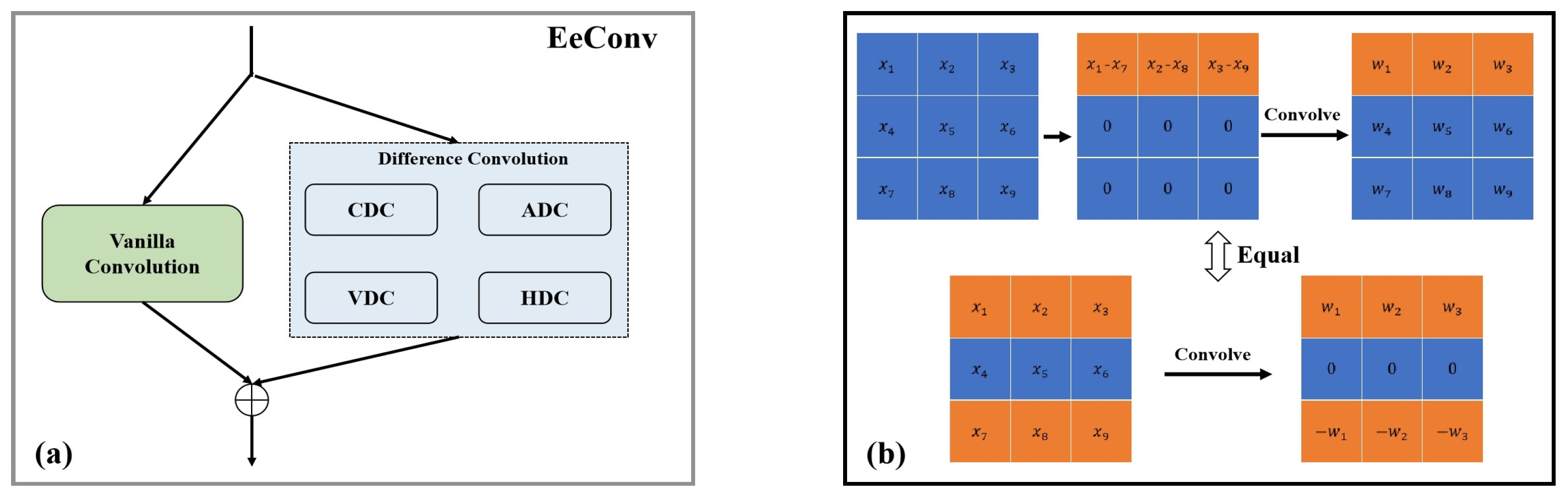
This paper discriminates the cloud and snow boundaries more accurately by using a difference convolution module named EeConv to extract high-frequency boundary information.

(4)

Considering the impact of two important geographical factors, slope and aspect, on the spatial distribution pattern of snow, this paper explores their potential as auxiliary information in deep learning and accomplishes the purpose of improving the accuracy of snow detection in mountainous regions, which which is often easy to be ignored in deep learning.

2. Methodology

A snow detection network (SD-GeoSTUNet) based on a Swin-Transformer and U-shaped dual-branch encoder structure with geographic information is proposed, which aims to discriminate the cloud and snow boundaries more accurately, minimize the occurrence of snow missing in hillside and valley areas, and make the segmentation results more refined.

In this part, the proposed SD-GeoSTUNet network architecture is first introduced, and then, focusing on two modules: FAM and residual layer embedded with EeConv.

2.1. Network Architecture

The overall architecture of SD-GeoSTUNet is shown in Figure 1, including CNN and Swin-T dual-branch encoders and a decoder. Among encoders, the CNN branch utilizes ResNet50 with residual structure as the backbone to reduce overfitting, speed up the calculation, and optimize the number of computation parameters [46]. The feature $X_1\in R^{4\times H\times W}$, which is composed of remote sensing image’s BGRI channels, is fed into a $7\times 7$ convolution layer with a stride step of 2 to change the number of channels and the shape to obtain the feature $F\in R^{64\times H/2\times W/2}$, and then a deeper feature $A_n$ is extracted through the residual layer embedded with EeConv, where $n=1,2,3,4$. The feature size of the nth residual layer output is $A_n\in R^{2^{n-1}{C}_2\times (H/2^{n+1})\times (W/2^{n+1})}$, where $C_2=128$. Simultaneously, considering the computing speed and the consumption of computing resources, the other encoder branch manipulates Swin-T as the backbone to extract the global feature, and the input feature image is $X_2\in R^{9\times H\times W}$, which is obtained by concatenating the remote sensing image’s BGRI channels and the five auxiliary geographic information maps along the channel dimension. Increasingly, $X_2$ is divided into $4\times 4$ image patches and after being flattened and projected into tokens by linear embedding, it will be sent to the standard Swin-T layer that combines Window Multi-head Self Attention (W-MSA) and Shifted Window Multi-head Self Attention (SW-MSA) for global feature extraction. The tokens obtained at each stage are converted to the designated channel, length, and width through patch merging before the Swin-T layer. There are four stages of Swin-T layers, and the numbers of layers in each stage are $2,2,6$, and 2, respectively. The output feature of each stage is $S_n\in R^{2^{n-1}{C}_1\times (H/2^{n+1})\times (W/2^{n+1})}$, of which $C_1=96$. Finally, the features extracted by the CNN branch and the features extracted by the Swin-T branch are sent to the FAM for feature fusion and high-dimensional information extraction. The feature size exported by FAM in each stage is $F_n\in R^{2^{n-1}{C}_2\times (H/2^{n+1})\times (W/2^{n+1})}$, where $C_2=128$.

In the decoding phase, the skip-connection layers similar to U-Net [47] are exploited to connect the encoder and decoder features. As the decoder layer illustrated in Figure 1a, initially, a $3\times 3$ convolution layer is introduced to reduce the number of channels, and then upsampling with a rate of 2 by pixelshuffle, which can significantly attenuate the occurrence of the checkerboard effect in transpose convolution [48], secondly, it concatenates $F_n$ from FAM in the channel dimension. Thirdly, a $3\times 3$ convolution layer, a Batch Normalization (BN) layer and a Rectified linear unit (Relu) activation layer are set for channel halving sequentially. After four iterations of the same decoder layer, the feature map is expanded to $F^{\prime }\in R^{64\times H/2\times W/2}$. Finally, the final prediction mask result is obtained after a $3\times 3$ convolution layer, a Relu layer, and a pixelshuffle with a rate of 2.

2.2. Feature Aggregation Module (FAM)

Several studies have proven that channel attention can improve the discrimination of objects with ambiguous boundaries and mitigate the omission of small-scale information [40,49]. By encoding the reliance on channel dimension, these mechanisms can strengthen the model’s capacity to distinguish features, thereby enabling the model to focus more effectively on detailed information extraction [50]. Therefore, to emphasize the most important and representative channels fed into the network and to better integrate the multi-scale features extracted from the CNN and Swin-T branches, this paper designs the FAM, which extracts the channel dependencies from the global features obtained from the Swin-T branch and then embeds the dependencies into the local features obtained from the CNN branch. This approach compensates for the limitations in local feature extraction and improves the network’s ability to delineate fine snow areas accurately. As illustrated in Figure 1b, a $1\times 1$ convolution layer is first applied to the features extracted by the Swin-T branch at stage n to obtain the features $S_n^{\prime }$ with the shape and size of $C_2\times H\times W$, where the channel number is the same as the feature $A_n$ that originates from the CNN branch. Then, the maximum and average vectors along the channel are calculated through the maximum-pool and average-pool layers, respectively. These vectors are subsequently fed into a shared fully connected layer $L_1$ to obtain the fully connected vectors, respectively. It should be noted that the fully connected layer $L_1$ is configured to halve the channel, resulting in the fully connected vectors $L_1\left(F_{A\&M}\right)\in R^{(C_2/2)\times 1\times 1}$, where $A=average-pool$ and $M=maximum-pool$. These vectors are then summed to produce the intermediate feature vector $F_{Mid}$. Next, the $F_{Mid}$ is sent to the shared fully connected layer $L_2$ to recover the number of channels to C₂. Ultimately, the Sigmoid function is applied to the output of $L_2$ to generate the channel dependency $F_{L_2}\in R^{C_2\times 1\times 1}$. The general formulations are summarized in Equations (1)–(4).

$$\begin{array}{c}\hfill F_A=AvgPool\left(S_n^{\prime }\right)\end{array}$$

(1)

$$\begin{array}{c}\hfill F_M=MaxPool\left(S_n^{\prime }\right)\end{array}$$

(2)

$$\begin{array}{c}\hfill F_{Mid}=\sigma (L_1\left(F_A\right)+L_1\left(F_M\right))\end{array}$$

(3)

$$\begin{array}{c}\hfill F_{L_2}=\delta (L_2\left(F_{Mid}\right))\end{array}$$

(4)

where $\sigma$ stands for the Relu function, $L_1$ refers to the fully connected layer 1, $L_2$ is the fully connected layer 2, and $\delta$ represents the Sigmoid function. At stage n, the features $A_n$ extracted by the CNN branch are multiplied by $F_{L_2}$ at the element level to obtain refined features, finally, the output features $F_n$ of FAM are obtained by adding refined features with $S_n$ and $A_n$. The formulation is expressed as Equation (5).

$$\begin{array}{c}\hfill F_n=S_n\oplus A_n\oplus (A_n\odot F_{L_2})\end{array}$$

(5)

2.3. Residual Layer Embedded with EeConv

Previous studies mainly adopted the vanilla convolution layer for feature extraction and search. However, the vanilla convolution is randomly initialized without any constraints, which may restrict its capacity for expression or modeling in large spaces [45]. Furthermore, several studies have shown that high-frequency information (such as edges and contours) is of great significance for restoring images captured in blurred scenes [51]. The difference convolution is mainly employed to convolve the weight with the pixel difference, allowing the network to pay more attention to the high-frequency texture information in the image. Therefore, the Edge-enhanced Convolution module (EeConv) [45] is designed to enhance the expression ability of the model for fuzzy cloud and snow boundaries. According to Figure 2a, EeConv includes vanilla convolution and difference convolution, in which difference convolution includes a central difference convolution (CDC) [52], an angular difference convolution (ADC) [52], a horizontal difference convolution (HDC) [45], and a vertical difference convolution (VDC) [45]. Take the vertical difference convolution as an example, as shown in Figure 2b. Firstly, the vertical gradient is calculated by computing the differences between the selected pixel pairs in the feature. Then, the vertical gradient is convoluted with the convolution kernel. This is also equivalent to directly applying the convolution kernel template to convolve with the original feature map, where the convolution kernel template must satisfy that the sum of the vertical weights equals zero. HDC shares a principle similar to VDC but calculates the difference in pixel pairs in the horizontal direction. Distinctly, the difference convolution explicitly encodes the gradient into the convolution layer, improving the model’s representation and generalization capacity. In our design, vanilla convolution is applied to obtain intensity-level information, while difference convolution is introduced to enhance gradient-level information. This paper adds the features learned from the two convolutions to obtain the output of EeConv, and the more complex feature fusion methods are not explored in depth. Several studies have proven that the convolution of parallel deployment can be simplified to a single standard convolution [45]. The calculation formulation is as Equation (6) [45].

$$\begin{array}{c}\hfill F_{out}=EeConv\left(F_{in}\right)=\sum _{i=1}^5{F}_{in}\ast K_i=F_{in}\left(\sum _{i=1}^5{K}_i\right)=F_{in}\ast K_{cut}\end{array}$$

(6)

where $F_{in}$ is the input feature, $K_i$ represents the convolution cores of VC, CDC, ADC, HDC, and VDC, respectively, ∗ signifies the convolution operation, and $K_{cut}$ donates the single standard convolution core after conversion.

In this paper, the idea of the ResNet residual block is regarded as a reference, and the EeConv is attached to the residual block structure. As depicted in Figure 1c, the input feature of each residual layer successively passes through the residual block consisting of a $1\times 1$ convolution layer, a $3\times 3$ convolution layer, and a $1\times 1$ convolution layer and then is fed into the EeConv to obtain the output feature of the residual layer, respectively. To prevent overfitting, a BN layer and a Relu activation layer are applied after each convolution. The residual layer numbers are $3,4,6$ and 3, respectively. By this, the features obtained by EeConv can be learned by subsequent residual blocks, significantly mitigating the loss of high-frequency information.

2.4. Experiment Settings

All experiments are implemented under the PyTorch [53] framework with Two Tesla V100-SXM2-32GB, and Python 3.11, PyTorch 2.1.2, and CUDA 12.2 are severed as the deep learning environments. The Adaptive Moment Estimation with Weight Decay (AdamW) [54] is used as the optimizer, which can adapt to the automatic adjustment of the learning rate of large datasets, ensuring model stability and preventing overfitting. The weight decay coefficient is set to $1\times e^{-4}$. The learning rate is adjusted using the Step Learning Rate Scheduler (StepLR), which updates the learning rate at specified intervals according to the learning rate attenuation coefficient. The calculation formulation is as Equation (7), where $l{r}_0$ represents the initial learning rate, $l{r}_n$ represents the learning rate of the nth round after updating, $\beta$ donates the attenuation coefficient, s refers to the update interval, and n is the training round. In this experiment, $l{r}_0$ is set to 0.001, $\beta$ is 0.8, s is 30, the batch size is 128, and the training epoch is 400.

$$\begin{array}{c}\hfill l{r}_n=l{r}_0\ast {\beta }^{\frac{n}{s}}\end{array}$$

(7)

To decrease the influence of the unbalanced category proportion in the dataset, which may cause the network to pay more attention to the larger proportion of categories, Equation (8) which combines Cross-Entropy Loss $L_{ce}$ with Dice Loss $L_{Dice}$ [55] is selected as the ultimate loss after the sensitivity experiment of a small amount of data, where L is the final loss.

$$\begin{array}{c}\hfill L=0.5\ast L_{ce}+0.5\ast L_{Dice}\end{array}$$

(8)

Due to a large amount of experimental data, the calculation time and cost are substantially increased. To address this issue, the experiments are conducted using the Automatic Mixed Precision (AMP) of PyTorch [53] in conjunction with gradient scaling mode, which could automatically train with the optimal data type, either float16 or float32, reducing memory occupancy and accelerating the training process.

2.5. Evaluation Metrics

Assessing the accuracy of test results is a crucial part of the cloud and snow detection assignment in remote sensing images using deep learning techniques. Take the label in the Levir_CS dataset as ground truth. Three commonly-used metrics, including Intersection over Union (IoU) [56], F1-score (F1) [57], and mean pixel accuracy (MPA) [58] are used as evaluation metrics in our experiments. IoU represents the ratio between the intersection and union of prediction values and ground truth. F1 can better measure missed and false detection, calculated by recall and precision. In particular, recall refers to the proportion of the number of positive samples correctly identified in the predicted values to the number of all positive samples; precision represents the proportion of correctly identified positive samples in all predicted positive samples. MPA denotes the proportion of pixels correctly classified in each category (the proportion of pixels correctly classified in the predicted category to the total pixels), and the average value obtained after accumulation. The calculation formulations are as in Equations (9)–(13):

$$\begin{array}{c}\hfill IoU={\displaystyle \frac{TP}{TP+FP+FN}}\end{array}$$

(9)

$$\begin{array}{c}\hfill Recall={\displaystyle \frac{TP}{TP+FN}}\end{array}$$

(10)

$$\begin{array}{c}\hfill Precision={\displaystyle \frac{TP}{TP+FP}}\end{array}$$

(11)

$$\begin{array}{c}\hfill F1=2\ast {\displaystyle \frac{Precision\times Recall}{Precision+Recall}}\end{array}$$

(12)

$$\begin{array}{c}\hfill MPA={\displaystyle \frac{1}{m}}\times {\displaystyle \frac{TP+TN}{TP+TN+FN+FP}}\end{array}$$

(13)

Among them, TP, TN, FP, and FN represent the number of true positive, true negative, false positive, and false negative targets generated after the detected target is compared with the ground truth, respectively, and m means the number of categories of all samples.

3. Data

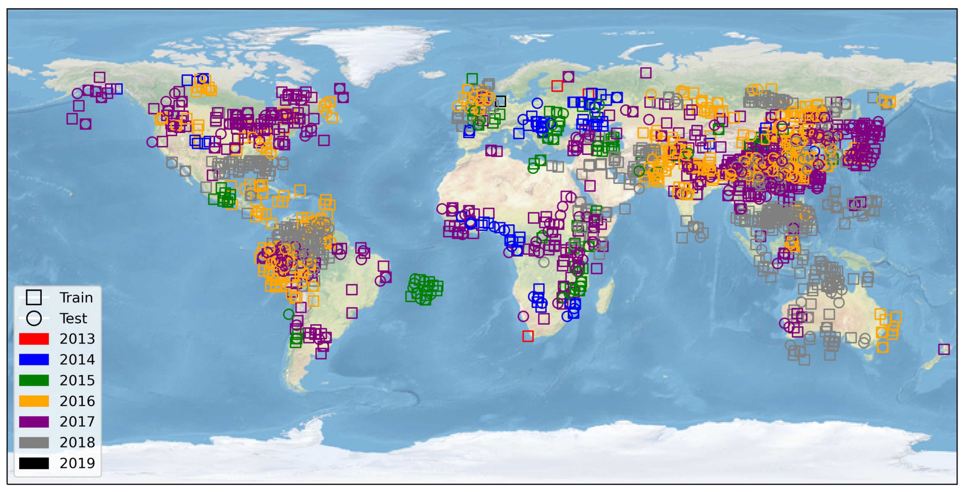
3.1. Data Introduction

The Levir_CS, released by Wu et al. [44] in 2021 and named by the author’s laboratory name “LEarning, VIsion, and Remote sensing laboratory”, is selected to meet the requirements for a large number of training data in Swin-T. Among them, C represents cloud and S means snow. Covering complex underlying surfaces of plains, mountains, deserts, and water bodies worldwide, and spanning a time range from 2013 to 2019, Levir_CS comprises 4168 Gaofen-1 Wide Field of View Sensor (WFV) images that are level-1A, without radiometric calibration, atmospheric correction, or systematic geometric correction process. These images can be downloaded from http://www.cresda.com/ (accessed on 28 February 2019). By 10× down-sampled from the original images, the spatial resolution of Levir_CS is 160 m, with a size of 1340 × 1200 pixels. All scenes in Levir_CS are manually annotated using Adobe Photoshop. Moreover, different from other cloud and snow datasets, each scene of Levir_CS only marks the background, cloud, and snow, thus minimizing the interference of other types of ground objects on cloud and snow recognition. In addition, geographic information, such as the latitude and longitude of each image, is retained, and the corresponding Digital Elevation Model(DEM) Terrain information is added based on their respective coordinates. The DEM is from the Space Shuttle Radar Topographic Survey Mission (SRTM), with a spatial resolution of 90 m [59]. Similar to the categories of Levir_CS, cloud or mountain shadows are considered part of the background in this paper.

3.2. Data Preprocessing

For the sake of fully utilizing the prior geographic knowledge in remote sensing images and further investigating the impact of terrain on snow detection, the slope and aspect will be calculated according to the DEM information of each image. Specifically, since DEM is in the World Geodetic System with the latest version (WGS-84), it is not convenient to calculate slope and aspect in this coordinate system, so this paper reprojects it to Lambert projection in batches with the help of ArcGIS 10.5 and then uses the slope and aspect calculation function to calculate the slope and aspect of DEM under Lambert projection, afterward, transform the slope and aspect to WGS-84 coordinate system to obtain the slope map $A_{Slope}$ and aspect map $A_{Aspect}$. In addition, given the coordinates of the upper-left corner, the number of rows and columns, and the projection information, are recorded on each scene, this paper generates the longitude map $A_{Long}$ and the latitude map $A_{Lat}$ with Equations (14) and (15), where y and x are the numbers of rows and columns of the image, respectively, and $r_{1,1}$, $r_{1,2}$, $r_{2,1}$, $r_{2,2}$ are the longitude and latitude resolution units on the x and y directions; moreover, $A_{Long}(0,0)$ and $A_{Lat}(0,0)$ mean the longitude and latitude coordinates of the upper-left corner of the image, respectively, and $A_{Long}(y,x)$ and $A_{Lat}(y,x)$ represent the longitude and latitude corresponding to row y and column x, respectively.

$$\begin{array}{c}\hfill A_{Long}(y,x)=A_{Long}(0,0)+y\ast r_{1,1}+x\ast r_{1,2}\end{array}$$

(14)

$$\begin{array}{c}\hfill A_{Lat}(y,x)=A_{Lat}(0,0)+y\ast r_{2,1}+x\ast r_{2,2}\end{array}$$

(15)

In this way, geospatial information can be integrated into the network as auxiliary knowledge to help detect snow from remote sensing images. All the detailed information on the feature maps is displayed in

Table 1. The detailed information on the feature maps.

Name	Source	Wavelength (µm)
B	remote sensing image’s blue band [44]	0.45~0.52
G	remote sensing image’s green band [44]	0.52~0.59
R	remote sensing image’s red band [44]	0.63~0.69
I	remote sensing image’s near-infrared band [44]	0.77~0.89
$A_{Alt}$	DEM [44]	/
$A_{Long}$	Calculate from remote sensing image’s projection	/
$A_{Lat}$	Calculate from remote sensing image’s projection	/
$A_{Slope}$	Calculate from DEM	/
$A_{Aspect}$	Calculate from DEM	/

.

Levir_CS faces a significant issue due to the imbalanced category proportions. To mitigate the interference of excessive backgrounds, this paper conducts annotation error detection, filtering, and dataset repartitioning before the experiments. Initially, 2065 images with predominantly background content and one image containing annotation errors are filtered out, leaving 2102 images for the experiment, as displayed in Figure 3. Among these, approximately 1404 scenes are completely snow-free, while 698 scenes include snow pixels. Despite deleting the background images, the remaining dataset is still much larger than other datasets in this field. Progressively, the images are randomly divided into a training set comprising 1472 scenes and a testing set with 630 scenes, following a 7:3 ratio. Furthermore, the images in the training set are regularly overlapped and sliced into image patches of 224 × 224 with an overlap rate of 10%. Then, 10% of the background patches are randomly adopted to reduce memory overhead and improve computational efficiency. This results in 35,693 small patches in the training set. Thirdly, all channels are normalized to [0, 1] to speed up convergence and facilitate network training. Specifically, the remote sensing image’s BGRI channels are divided by 1023 for the radiation resolution is 10-bit, the DEM channels are divided by 10,000, the longitude channels are divided by 360 after adding 180, the latitude channels are divided by 180 after adding 90, the slope channels are divided by 90, and the aspect channels are divided by 360. Before training, data augmentation techniques, such as randomly flipping images horizontally and vertically, are implemented to enhance the robustness of the network and increase the diversity of training images.

4. Results

This part conducts two types of experiments: ablation experiments and comparative experiments. The ablation experiments aim to verify the rationality and effectiveness of network structure, module components, and auxiliary geographic information for snow recognition. Furthermore, the comparative experiments are designed to highlight the advantages of the proposed model compared with other semantic segmentation models for snow detection on the Levir_CS dataset.

4.1. Ablation Experiment

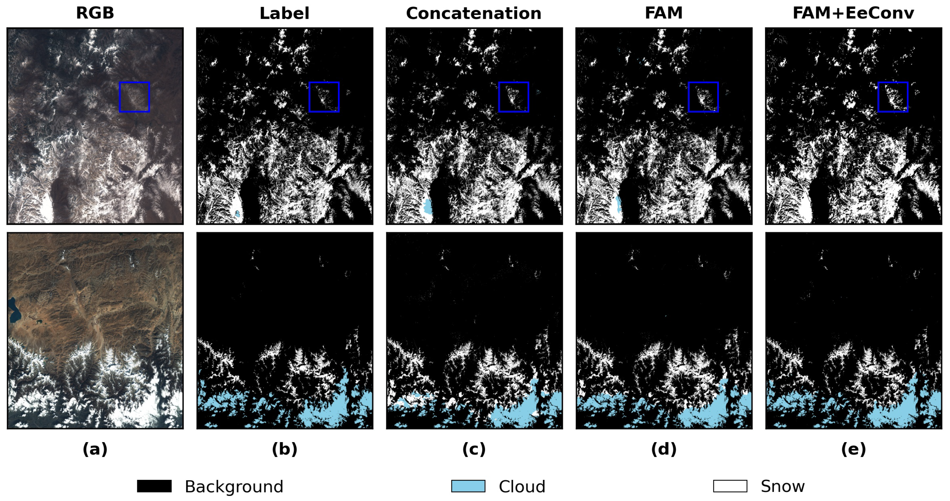
4.1.1. Ablation Experiment of Network Structure and Module Components

To evaluate the effectiveness of the proposed network and to better quantify the contribution of each module to snow recognition, ablation studies are designed on the network structure and modules. The results are compared from evaluation metrics and visualization maps. The features fed into the CNN branch are remote sensing image’s BGRI, while in the Swin-T branch are remote sensing image’s BGRI and five geographic maps illustrated in the data preprocessing. In this experiment, IoU, F1, and MPA are used as evaluation metrics, where $F1\_c$ represents the F1 of the cloud, $F1\_s$ means the F1 score of snow, $IoU\_c$ is the IoU of the cloud, and $IoU\_s$ donates the IoU of snow. All the metrics are exhibited in

Table 2. Evaluation metrics of network structure and module ablation experiments.

Name	IoU_c	IoU_s	F1_c	F1_s	MPA
CNN	85.31%	74.63%	91.69%	81.51%	89.86%
Swin-T	87.84%	75.74%	92.77%	83.01%	90.29%
CNN+Swin-T (Concatenation)	88.75%	76.36%	93.85%	83.93%	91.24%
CNN+Swin-T+FAM	89.63%	77.25%	94.67%	84.69%	92.01%
CNN+Swin-T+FAM+EeConv (SD-GeoSTUNet)	90.37%	78.08%	95.25%	85.07%	92.89%

, in which the optimal values have been bolded.

To investigate the individual contributions of the CNN branch and Swin-T branch to snow detection and their combined efficiency, comparisons between different network structures are made. As shown in the first three rows of Table 2, the metrics for the dual-branch network surpass those of any single-branch network. Furthermore, only by simply concatenating the features from the CNN and Swin-T along the channel dimension, the $MPA$ rises by 0.95%, surpassing the highest performance achieved by the single-branch network notably. It is evident that the dual-branch network effectively integrates the strengths of the CNN branch and the Swin-T branch in extracting both local detail features and global context correlation features, which create the framework foundation for subsequent investigations on enhancing the performance of the dual-branch network.

According to the last three rows of Table 2, module ablation experiments on the FAM and EeConv are conducted based on the dual-branch network structure. Our motivation for incorporating FAM is to better integrate the features extracted by the dual-branch encoder, alleviate the loss of detail information, and reduce the omission of small snow areas; after introducing the EeConv, the model will be inclined to pay more attention to the high-frequency information of the boundary through difference convolution, impairing the uncertainty of the cloud and snow boundary, and decreasing the miscalculation and omission of snow areas through more accurate positioning of the boundary. Compared to Figure 4c,d, the network with FAM effectively alleviates the phenomenon where clouds are misjudged as snow in the second-row scene; moreover, more thin snow is detected in Figure 4d in the blue frame of the first-row scene in comparison to the network concatenating dual-branch feature simply. The metrics $IoU\_c$, $IoU\_s$, $F1\_c$, $F1\_s$, and $MPA$, when combined with the FAM module, have a rise of 0.88%, 0.89%, 0.82%, 0.76%, and 0.77%, respectively. By equipping with the EeConv displayed in Figure 4e, the misjudgment of cloud and snow is further minimized, and more thin snow is detected in the blue frame than in Figure 4d, depicting a snow boundary contour that closely resembles the one shown in Figure 4a RGB images. Furthermore, the metrics $IoU\_c$, $IoU\_s$, $F1\_c$, $F1\_s$, and $MPA$ all achieve their highest values in all experiments, which are 90.37%, 78.08%, 95.25%, 85.07%, and 92.89%, respectively. These values are enhanced by 0.74%, 0.83%, 0.58%, 0.38%, and 0.88% compared to the network without EeConv. It demonstrates that the EeConv has better performance in discriminating the boundary between the cloud and snow areas, and it helps to preserve more thin detailed snow, thereby improving the depiction of the border contours. In summary, the SD-GeoSTUNet, when combined with FAM and EeConv, exhibits enhanced capabilities in segmenting clouds and snow and detecting more snow details.

4.1.2. Ablation Experiment of Geographic Information

In order to quantitatively and qualitatively grasp the contribution of slope and aspect to snow extraction in mountainous images, this part mainly executes ablation experiments of the following three schemes according to the input feature of the Swin-T branch: (1) $BGRI$, (2) $BGRI+A_{Alt}+A_{Long}+A_{Lat}$, (3) $BGRI+A_{Alt}+A_{Long}+A_{Lat}+A_{Slope}+A_{Aspect}$. Given that previous studies have proven the effectiveness of altitude, longitude, and latitude for snow recognition [44], this study takes them as a combination and does not evaluate the impact of a single feature on the results in detail. The feature coding sequence is concatenated along the channel dimension in the order of $A_{Alt},A_{Long},A_{Lat},A_{Slope},A_{Aspect}$.

Table 3. Evaluation metrics of different geographic information feature combinations.

BGRI	${\mathit{A}}_{\mathit{Alt}}+{\mathit{A}}_{\mathit{Long}}+{\mathit{A}}_{\mathit{Lat}}$	${\mathit{A}}_{\mathit{Slope}}+{\mathit{A}}_{\mathit{Aspect}}$	IoU_c	IoU_s	F1_c	F1_s	MPA
✓			88.57%	77.14%	93.98%	83.91%	91.10%
✓	✓		90.02%	78.22%	94.61%	85.26%	93.01%
✓	✓	✓	90.37%	78.08%	95.25%	85.07%	92.89%

displays the $IoU$, $F1$, and $MPA$ of different geographic information feature combination ablation experiments. The optimal values have been bolded.

According to Table 3, the metrics for Experiment 2 and Experiment 3 are higher than those for Experiment 1, indicating that the addition of geographic information can contribute to detecting snow more accurately, which is consistent with the conclusion of Wu et al. that geographic information can improve the accuracy of cloud and snow detection [44], Therefore, it is feasible to incorporate geographic information to improve the accuracy of cloud and snow segmentation. The $IoU\_c$ and $F1\_c$ attain the highest values across all tests in Experiment 3, specifically 90.37% and 95.25%, respectively. However, the highest metrics for the snow are achieved in Experiment 2, with the $IoU\_s$, $F1\_s$, and $MPA$ scores being 78.22%, 85.26%, and 93.01%, respectively, which are 0.14%, 0.19%, and 0.12% higher than those in Experiment 3. Figure 5 shows the snow detection result of different geographic information feature combination schemes and three enlarged views (marked with blue, green, and red boxes) under the mountain regions with the geographical coordinates of 128°E and 44.7°N. The results of Experiment 1, Experiment 2, and Experiment 3 are displayed in columns (c), (d), and (e), respectively. The observation reveals that all experimental results display the primary contour boundary of snow, and the coverage of snow detection in (d) is considerably broader compared to (c). By incorporating slope and aspect, the determined snow cover area in (e) is remarkably expanded compared to (d), which suggests that the network has considered the potential influence of slope and aspect changes on snow detection when extracting snow information features. The blue, green, and red boxes indicate the enlarged scenes of complicated topography consisting of hillsides and valleys. The snow metrics in Experiment 2 are higher than those in Experiment 3, and the possible reasons are as follows: After enlarging and carefully observing the RGB and label, it is challenging to visually find the snow in these terrains in (a) RGB true color images, making the snow in the viewable areas surrounding the terrains annotated in the label, while some invisible pixels may be marked as background. As the network detects the snow in those complex terrains, the background and snow metrics, such as IoU, will be slightly lower when calculating the metrics. That is why the snow indexes decline but the cloud does not. Nevertheless, the visualization results illustrate that the slope and aspect can notably decrease the omission of snow in hillside and valley areas.

4.2. Comparative Experiment

In this part, several models are selected to conduct comparative experiments to validate the actual performance of our model, including the classical deep learning semantic segmentation models PSPNet [60], U-Net [47], Segformer [61] and the models CDNetV2 [40] and GeoInfoNet [44], which have been especially used for cloud and snow detection tasks; the source codes have been available online in recent years, and except from the Segformer they adopt transformer architecture, and all the others adopt CNN architecture. With the SD-GeoSTUNet proposed, a total of six experiments are carried out. In order to ensure that the preconditions for comparison are consistent, all the models are trained based on the same dataset and encode nine features, including remote sensing image’s BGRI bands and five geographical features. Next, the performance and effectiveness of cloud and snow detection for each model are assessed based on evaluation metrics and visualization results.

4.2.1. Accuracy Evaluation

Table 4. Evaluation metrics of different models.

Model	IoU_c	IoU_s	F1_c	F1_s	MPA	Parameter (M)
PSPNet 1	85.57%	74.37%	89.87%	81.20%	85.25%	65.703
U-Net 2	88.76%	77.08%	93.17%	83.89%	91.29%	17.267
GeoInfoNet 3	89.74%	77.81%	94.78%	84.69%	92.14%	29.324
CDNetV2 4	89.01%	77.45%	94.08%	84.53%	91.68%	67.677
Segformer 5	87.99%	75.99%	92.98%	83.04%	90.32%	84.614
SD-GeoSTUNet	90.37%	78.08%	95.25%	85.07%	92.89%	77.749

¹ The code can be found https://github.com/Lextal/pspnet-pytorch (accessed on 3 April 2024). ² The code can be found https://github.com/WZMIAOMIAO/deep-learning-for-image-processing/tree/master/pytorch_segmentation/unet (accessed on 16 December 2023). ³ The code and data can be found https://github.com/permanentCH5/GeoInfoNet (accessed on 10 November 2023). ⁴ The code can be found https://github.com/nkszjx/CDnetV2-pytorch-master (accessed on 16 April 2024). ⁵ The code can be found https://github.com/lucidrains/segformer-pytorch (accessed on 16 April 2024).

represents the evaluation metrics of the prediction results of each model. On the basis of all evaluation indexes, the rank of the model performance is as follows: SD-GeoSTUNet > GeoInfoNet > CDNetV2 > U-Net > Segformer > PSPNet. It is evident that the SD-GeoSTUNet shows optimal performance in several key indexes, achieving 90.37%, 78.08%, 95.25%, 85.07%, and 92.89% in $IoU\_c$, $IoU\_s$, $F1\_c$, $F1\_s$, and $MPA$, respectively. The SD-GeoSTUNet outperformed the GeoInfoNet, which ranked second in the comprehensive score, with improvements of 0.63%, 0.27%, 0.47%, 0.38%, and 0.75% in $IoU\_c$, $IoU\_s$, $F1\_c$, $F1\_s$, and $MPA$, respectively. It also indicates that the dual-branch architecture network combined with CNN and Swin-T can enhance the cloud and snow detection on the Levir_CS dataset compared with the single-branch encoder architecture network. However, it is worth noting that the $IoU\_c$ and $F1\_c$, have increased remarkably, which proves that the SD-GeoSTUNet can detect the cloud better, but the $IoU\_s$ and $F1\_s$ have not shown a notable increase, which could be attributed to the label issues in mountainous areas, as discussed in Section 4.1.2. The optimal values have been bolded.

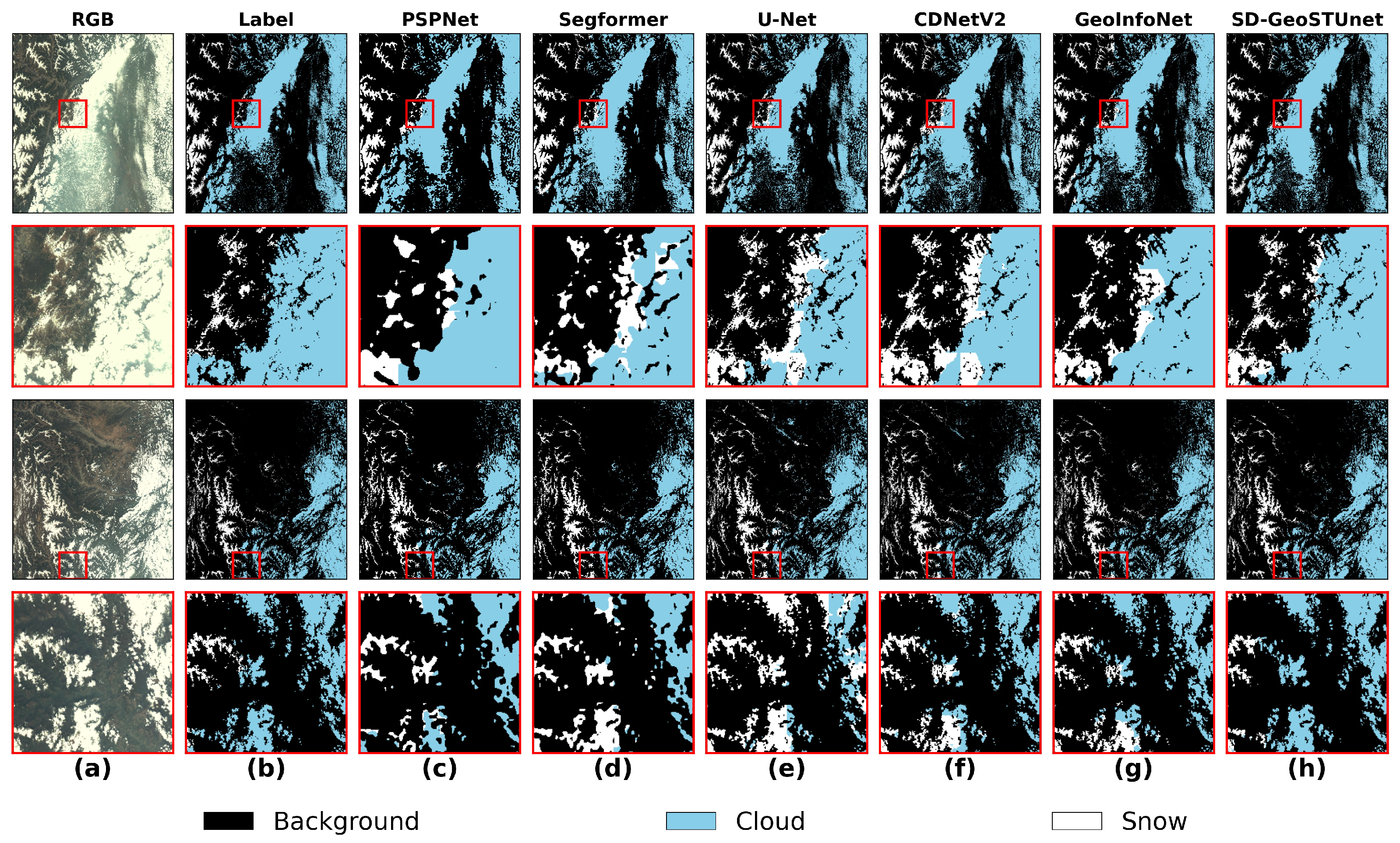
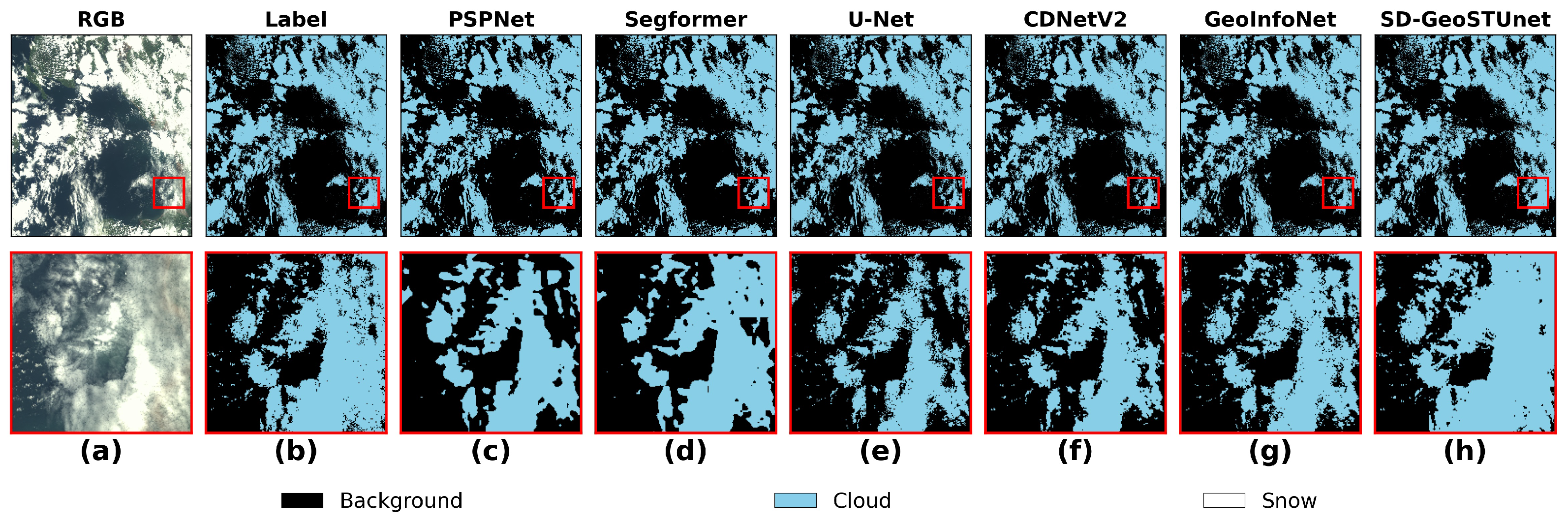
4.2.2. Visualization Results

Figure 5, Figure 6 and Figure 7 display the segmentation results of each model for cloud and snow under several scenarios, including coexistence, pure snow, and pure cloud, excluding the background class, respectively. It can be observed that all the models can detect the approximate cloud and snow contour overall, exhibiting a certain cloud and snow segmentation effect. However, the performance of both PSPNet and Segformer is notably inferior compared to other models, which only manage to capture the general outline of objects and obtain rougher borders, failing to accurately segment detailed small cloud and snow patches. In detail, PSPNet introduces the pyramid pooling module, which uses dilated convolution to capture multi-scale context information [60], but PSPNet will lose many details due to its special convolution principle and the lack of branches connected across layers to integrate the details of different layers in the up-sampling process. Compared with PSPNet, Segformer enhances the decoder module and utilizes a Multi-Layer Perceptron (MLP) [61] to restore the up-sample functionality, resulting in more detailed information being reserved. Nevertheless, during the encoder phase, the utilization of a solitary transformer structure and self-attention mechanism for feature extraction may result in the neglect of certain local intricacies while computing long-range dependencies.

Due to the extremely high spectral, texture, and shape similarity of cloud and snow, its accurate segmentation has always been a challenge [11]. In the results displayed in Figure 6, SD-GeoSTUNet shows evident superiority to other models in cloud and snow boundary discrimination, which is the most consistent with the label. PSPNet and Segformer exhibit worse extraction of detailed contours for cloud and snow targets, as well as the differentiation between cloud and snow boundaries. Meanwhile, U-Net, CDNetV2, and GeoInfoNet have different degrees of cloud and snow misjudgment, resulting in blurred boundary distinction.

Just as the label shows fewer thin snow pixels in mountainous, after encoding nine features including slope and aspect, it can be seen from Figure 7 that the snow pixels identified by all models are more than labeled, with the SD-GeoSTUNet being the most similar to RGB. This demonstrates that utilizing the topographical characteristics is indeed effective in extracting snow pixels from mountain slopes and valleys. In addition, PSPNet, U-Net, CDNetV2, and GeoInfoNet have identified snow as clouds in various positions, but do not appear in SD-GeoSTUNet.

In addition to correctly distinguishing cloud and snow boundaries and identifying snow cover, accurate cloud extraction is also vital. From the results depicted in Figure 8, SD-GeoSTUNet achieves the best cloud detection, which decreases the loss of thin clouds to a great extent and is beyond the reach of the other model. Although it can be observed that the Segformer is capable of identifying thin clouds, it has limited proficiency in smoothing the edges. What is more, compared with the label, U-Net, CDNetV2, and GeoInfoNet omit many cloud pixels, especially in thin clouds, but the edge is smoother than Segformer. This result proves that SD-GeoSTUNet, combining CNN and transformer structures, could effectively leverage their complementary strengths and excavate more detailed information.

5. Discussion

Compared with traditional physical methods, snow detection from remote sensing images based on deep learning can increase automation and efficiency by reducing the time and steps required to process numerous remote sensing images [30] and achieve higher accuracy [32]. Moreover, it is convenient for deep learning-based methods to integrate with various types of data [62,63], giving play to the synergy of that in snow recognition. Based on the advantages mentioned above, this paper proposes SD-GeoSTUNet to improve the performance of snow detection from Gaofen-1 images, particularly in thin snow detection and cloud and snow boundary segmentation. This is achieved by making improvements to various modules: the devised FAM can strengthen the model’s capacity to fuse features by encoding the channel dimension reliance between the CNN branch and Swin-T branch, and the EeConv can maximize the retention of outline information by focusing more on high-frequency edge differences. Motivated by the terrain affecting the spatial distribution of snow [64,65], geographical information like slope and aspect are adopted to promote snow extraction in mountainous areas, where the phenomenon of snow omission is distinctly mitigated compared to the experiment without encoding slope and aspect information and label. As elaborated in Section 4.1.2, we discover that after encoding the slope and aspect, the cloud metrics will increase, which is consistent with Wu et al.’s finding that geographic information can aid in the cloud and snow identification [44]. However, the snow metrics slightly decrease. Upon further analysis, we find that some snow pixels surrounding the terrains may have been marked as background. Given the large magnitude of the dataset and the lack of a shortwave infrared band (cirrus band, 1.6 µm) in Gaofen-1 [66], it is more challenging to assist in the manual labeling of snow by calculating the snow index NDSI or combining the cirrus, green, and blue bands. Despite this, with the assistance of geographic information and the powerful learning ability of the deep learning model, we realize the detection of unlabeled snow. The visual effect is closer to the RGB image, while there is a decrease in metrics. This has inspired us to consider combining geographic information, meteorological data, and other relevant data for more accurate snow identification when the bands of remote sensing images are not sufficient. Therefore, this paper can also serve as a reference for producing higher-quality snow labels in the future.

Although the SD-GeoSTUNet has achieved remarkable snow extraction results from the Levir_CS dataset, it still has some limitations and shortcomings. Firstly, besides the Levir_CS, at present, there are relatively few large-scale cloud and snow datasets with image geographic information that can be used for cloud and snow semantic segmentation tasks [30,38,39], which limits the opportunity to make data comparison experiments, and limits the application of geographic information in this task to a certain extent. In addition, this paper lacks consideration of the effects of model parameters.

In the future, reducing the number of model parameters under the premise of ensuring the detection accuracy may be a main goal. In addition, integrating various surface and meteorological variables, such as surface temperature and near-surface temperature [67], which could provide more information about snow formation and melting, holds promise, and attribute information such as solar angle and imaging time can also be considered for this task.

6. Conclusions

This paper proposes a snow detection network based on a Swin-Transformer and U-shaped dual-branch encoder structure with geographic information, which aims to detect snow more accurately, especially in mountain areas, and segment cloud and snow boundaries more precisely in the Gaofen-1 WFV dataset named Levir_CS. Firstly, the network combines the CNN and Swin-T branches as encoders to extract features in parallel. Through the FAM, the advantages of CNN and Swin-T in extracting local features and global context features are efficiently integrated, which enhances the ability of network fusion features and improves the attention of the network to detailed information. Then, the EeConv is attached to the CNN branch to extract high-frequency boundary information, to achieve more accurate cloud and snow boundary segmentation and thin snow detection. More importantly, to investigate the potential contribution of geographic information to the field of snow detection in deep learning, this paper calculates the slope and aspect maps of each scene from the Levir_CS dataset after data preprocessing and then encodes them with altitude, longitude, and latitude into five geographic information maps, which are sent to the Swin-T branch for feature extraction. Ultimately, more snow in mountainous areas is successfully extracted. Following the ablation experiment and comparative experiment, our method demonstrates superior performance in both visualization and quantitative evaluation than other methods, and the primary conclusions can be outlined as follows:

(1)

The respective advantages of CNN and Swin-T in feature extraction are combined by a dual-branch encoder structure in parallel. By concatenating the dual-branch features along channels, the MPA reached 91.24%, which is 0.95% higher than the best performance of the single-branch network. SD-GeoSTUNet can deeply extract the detailed information between the features by combining the CNN and Swin-T through FAM and reserving the high-frequency edge information by EeConv.

(2)

The SD-GeoSTUNet model improves when encoding altitude, longitude, and latitude with the remote sensing image’s BGRI. Furthermore, encoding the slope and aspect further improves the snow detection performance in hillside and valley areas.

(3)

Compared with other existing CNN framework models or transformer framework models, SD-GeoSTUNet shows the best cloud and snow detection performance, with more clear and accurate detection results and the least thin cloud and snow omission, and achieves the highest $IoU\_c$, $IoU\_s$, $F1\_c$, $F1\_s$, and $MPA$, which are 90.37%, 78.08%, 95.25%, 85.07%, and 92.89%, respectively, outperform other models profoundly.

References

1. Zhang, T. Influence of the seasonal snow cover on the ground thermal regime: An overview. Rev. Geophys. 2005, 43, 1–23. [Google Scholar] [CrossRef]
2. Zhang, Y. Multivariate Land Snow Data Assimilation in the Northern Hemisphere: Development, Evaluation and Uncertainty Quantification of the Extensible Data Assimilation System. Ph.D. Thesis, The University of Texas at Austin, Austin, TX, USA, 2015. [Google Scholar]
3. Wijngaard, R.R.; Biemans, H.; Lutz, A.F.; Shrestha, A.B.; Wester, P.; Immerzeel, W. Climate change vs. socio-economic development: Understanding the future South Asian water gap. Hydrol. Earth Syst. Sci. 2018, 22, 6297–6321. [Google Scholar] [CrossRef]
4. Barnett, T.P.; Adam, J.C.; Lettenmaier, D.P. Potential impacts of a warming climate on water availability in snow-dominated regions. Nature 2005, 438, 303–309. [Google Scholar] [CrossRef]
5. Kraaijenbrink, P.D.A.; Stigter, E.E.; Yao, T.; Immerzeel, W.W. Climate change decisive for Asia’s snow meltwater supply. Nat. Clim. Chang. 2021, 11, 591–597. [Google Scholar] [CrossRef]
6. Morin, S.; Samacoïts, R.; François, H.; Carmagnola, C.M.; Abegg, B.; Demiroglu, O.C.; Pons, M.; Soubeyroux, J.M.; Lafaysse, M.; Franklin, S.; et al. Pan-European meteorological and snow indicators of climate change impact on ski tourism. Clim. Serv. 2021, 22, 100215. [Google Scholar] [CrossRef]
7. Deng, G.; Tang, Z.; Hu, G.; Wang, J.; Sang, G.; Li, J. Spatiotemporal dynamics of snowline altitude and their responses to climate change in the Tienshan Mountains, Central Asia, During 2001–2019. Sustainability 2021, 13, 3992. [Google Scholar] [CrossRef]
8. Ayub, S.; Akhter, G.; Ashraf, A.; Iqbal, M. Snow and glacier melt runoff simulation under variable altitudes and climate scenarios in Gilgit River Basin, Karakoram region. Model. Earth Syst. Environ. 2020, 6, 1607–1618. [Google Scholar] [CrossRef]
9. Tang, Z.; Wang, X.; Deng, G.; Wang, X.; Jiang, Z.; Sang, G. Spatiotemporal variation of snowline altitude at the end of melting season across High Mountain Asia, using MODIS snow cover product. Adv. Space Res. 2020, 66, 2629–2645. [Google Scholar] [CrossRef]
10. Huang, N.; Shao, Y.; Zhou, X.; Fan, F. Snow and ice disaster: Formation mechanism and control engineering. Front. Earth Sci. 2023, 10, 1019745. [Google Scholar] [CrossRef]
11. Tsai, Y.L.S.; Dietz, A.; Oppelt, N.; Kuenzer, C. Remote sensing of snow cover using spaceborne SAR: A review. Remote Sens. 2019, 11, 1456. [Google Scholar] [CrossRef]
12. Tang, Z.; Wang, J.; Li, H.; Liang, J.; Li, C.; Wang, X. Extraction and assessment of snowline altitude over the Tibetan plateau using MODIS fractional snow cover data (2001 to 2013). J. Appl. Remote Sens. 2014, 8, 084689. [Google Scholar] [CrossRef]
13. Wang, J.; Tang, Z.; Deng, G.; Hu, G.; You, Y.; Zhao, Y. Landsat satellites observed dynamics of snowline altitude at the end of the melting season, Himalayas, 1991–2022. Remote Sens. 2023, 15, 2534. [Google Scholar] [CrossRef]
14. Hall, D.K.; Riggs, G.A.; Salomonson, V.V. Development of methods for mapping global snow cover using moderate resolution imaging spectroradiometer data. Remote Sens. Environ. 1995, 54, 127–140. [Google Scholar] [CrossRef]
15. Hall, D.K.; Riggs, G.A.; Salomonson, V.V.; DiGirolamo, N.E.; Bayr, K.J. MODIS snow-cover products. Remote Sens. Environ. 2002, 83, 181–194. [Google Scholar] [CrossRef]
16. Zhu, Z.; Woodcock, C.E. Automated cloud, cloud shadow, and snow detection in multitemporal Landsat data: An algorithm designed specifically for monitoring land cover change. Remote Sens. Environ. 2014, 152, 217–234. [Google Scholar] [CrossRef]
17. Zhu, Z.; Wang, S.; Woodcock, C.E. Improvement and expansion of the Fmask algorithm: Cloud, cloud shadow, and snow detection for Landsats 4–7, 8, and Sentinel 2 images. Remote Sens. Environ. 2015, 159, 269–277. [Google Scholar] [CrossRef]
18. Gascoin, S.; Grizonnet, M.; Bouchet, M.; Salgues, G.; Hagolle, O. Theia Snow collection: High-resolution operational snow cover maps from Sentinel-2 and Landsat-8 data. Earth Syst. Sci. Data 2019, 11, 493–514. [Google Scholar] [CrossRef]
19. Wang, X.; Wang, J.; Li, H.; Hao, X. Combination of NDSI and NDFSI for snow cover mapping in a mountainous and forested region. Natl. Remote. Sens. Bull. 2017, 21, 310–317. [Google Scholar] [CrossRef]
20. Wang, L.; Chen, Y.; Tang, L.; Fan, R.; Yao, Y. Object-based convolutional neural networks for cloud and snow detection in high-resolution multispectral imagers. Water 2018, 10, 1666. [Google Scholar] [CrossRef]
21. Deng, G.; Tang, Z.; Dong, C.; Shao, D.; Wang, X. Development and Evaluation of a Cloud-Gap-Filled MODIS Normalized Difference Snow Index Product over High Mountain Asia. Remote Sens. 2024, 16, 192. [Google Scholar] [CrossRef]
22. Li, P.F.; Dong, L.M.; Xiao, H.C.; Xu, M.L. A cloud image detection method based on SVM vector machine. Neurocomputing 2015, 169, 34–42. [Google Scholar] [CrossRef]
23. Ishida, H.; Oishi, Y.; Morita, K.; Moriwaki, K.; Nakajima, T.Y. Development of a support vector machine based cloud detection method for MODIS with the adjustability to various conditions. Remote Sens. Environ. 2018, 205, 390–407. [Google Scholar] [CrossRef]
24. Hollstein, A.; Segl, K.; Guanter, L.; Brell, M.; Enesco, M. Ready-to-Use Methods for the Detection of Clouds, Cirrus, Snow, Shadow, Water and Clear Sky Pixels in Sentinel-2 MSI Images. Remote Sens. 2016, 8, 666. [Google Scholar] [CrossRef]
25. Ghasemian, N.; Akhoondzadeh, M. Introducing two Random Forest based methods for cloud detection in remote sensing images. Adv. Space Res. 2018, 62, 288–303. [Google Scholar] [CrossRef]
26. Tuia, D.; Kellenberger, B.; Pérez-Suey, A.; Camps-Valls, G. A deep network approach to multitemporal cloud detection. In Proceedings of the IGARSS 2018–2018 IEEE International Geoscience and Remote Sensing Symposium, Valencia, Spain, 22–27 July 2018; pp. 4351–4354. [Google Scholar]
27. Han, W.; Zhang, X.H.; Wang, Y.; Wang, L.Z.; Huang, X.H.; Li, J.; Wang, S.; Chen, W.T.; Li, X.J.; Feng, R.Y.; et al. A survey of machine learning and deep learning in remote sensing of geological environment: Challenges, advances, and opportunities. Isprs J. Photogramm. Remote Sens. 2023, 202, 87–113. [Google Scholar] [CrossRef]
28. Long, J.; Shelhamer, E.; Darrell, T. Fully convolutional networks for semantic segmentation. In Proceedings of the IEEE Conference on Computer Vision and Pattern Recognition, Boston, MA, USA, 7–12 June 2015; pp. 3431–3440. [Google Scholar]
29. Zheng, K.; Li, J.; Yang, J.; Ouyang, W.; Wang, G.; Zhang, X. A cloud and snow detection method of TH-1 image based on combined ResNet and DeeplabV3+. Acta Geod. Et Cartogr. Sin. 2020, 49, 1343. [Google Scholar]
30. Zhang, G.B.; Gao, X.J.; Yang, Y.W.; Wang, M.W.; Ran, S.H. Controllably Deep Supervision and Multi-Scale Feature Fusion Network for Cloud and Snow Detection Based on Medium- and High-Resolution Imagery Dataset. Remote Sens. 2021, 13, 4805. [Google Scholar] [CrossRef]
31. Yin, M.J.; Wang, P.; Ni, C.; Hao, W.L. Cloud and snow detection of remote sensing images based on improved Unet3+. Sci. Rep. 2022, 12, 14415. [Google Scholar] [CrossRef]
32. Lu, Y.; James, T.; Schillaci, C.; Lipani, A. Snow detection in alpine regions with Convolutional Neural Networks: Discriminating snow from cold clouds and water body. GIScience Remote Sens. 2022, 59, 1321–1343. [Google Scholar] [CrossRef]
33. Vaswani, A.; Shazeer, N.; Parmar, N.; Uszkoreit, J.; Jones, L.; Gomez, A.N.; Kaiser, Ł.; Polosukhin, I. Attention is all you need. In Proceedings of the 31st Conference on Neural Information Processing Systems (NIPS 2017), Long Beach, CA, USA, 4–9 December 2017; Volume 30. [Google Scholar]
34. Dosovitskiy, A.; Beyer, L.; Kolesnikov, A.; Weissenborn, D.; Zhai, X.; Unterthiner, T.; Dehghani, M.; Minderer, M.; Heigold, G.; Gelly, S.; et al. An image is worth 16 × 16 words: Transformers for image recognition at scale. arXiv 2020, arXiv:2010.11929. [Google Scholar]
35. Hu, K.; Zhang, E.; Xia, M.; Weng, L.; Lin, H. Mcanet: A multi-branch network for cloud/snow segmentation in high-resolution remote sensing images. Remote Sens. 2023, 15, 1055. [Google Scholar] [CrossRef]
36. Ma, J.; Shen, H.; Cai, Y.; Zhang, T.; Su, J.; Chen, W.H.; Li, J. UCTNet with dual-flow architecture: Snow coverage mapping with Sentinel-2 satellite imagery. Remote Sens. 2023, 15, 4213. [Google Scholar] [CrossRef]
37. Liu, Z.; Lin, Y.; Cao, Y.; Hu, H.; Wei, Y.; Zhang, Z.; Lin, S.; Guo, B. Swin transformer: Hierarchical vision transformer using shifted windows. In Proceedings of the IEEE/CVF International Conference on Computer Vision, Montreal, BC, Canada, 11–17 October 2021; pp. 10012–10022. [Google Scholar]
38. Hughes, M.J.; Hayes, D.J. Automated detection of cloud and cloud shadow in single-date Landsat imagery using neural networks and spatial post-processing. Remote Sens. 2014, 6, 4907–4926. [Google Scholar] [CrossRef]
39. Wang, Y.; Su, J.; Zhai, X.; Meng, F.; Liu, C. Snow Coverage Mapping by Learning from Sentinel-2 Satellite Multispectral Images via Machine Learning Algorithms. Remote Sens. 2022, 14, 782. [Google Scholar] [CrossRef]
40. Guo, J.; Yang, J.; Yue, H.; Tan, H.; Hou, C.; Li, K. CDnetV2: CNN-based cloud detection for remote sensing imagery with cloud-snow coexistence. IEEE Trans. Geosci. Remote Sens. 2020, 59, 700–713. [Google Scholar] [CrossRef]
41. Wang, Y.; Gu, L.; Li, X.; Gao, F.; Jiang, T. Coexisting cloud and snow detection based on a hybrid features network applied to remote sensing images. IEEE Trans. Geosci. Remote Sens. 2023, 61, 5405515. [Google Scholar] [CrossRef]
42. Kormos, P.R.; Marks, D.; McNamara, J.P.; Marshall, H.P.; Winstral, A.; Flores, A.N. Snow distribution, melt and surface water inputs to the soil in the mountain rain-snow transition zone. J. Hydrol. 2014, 519, 190–204. [Google Scholar] [CrossRef]
43. Hartman, M.D.; Baron, J.S.; Lammers, R.B.; Cline, D.W.; Band, L.E.; Liston, G.E.; Tague, C. Simulations of snow distribution and hydrology in a mountain basin. Water Resour. Res. 1999, 35, 1587–1603. [Google Scholar] [CrossRef]
44. Wu, X.; Shi, Z.W.; Zou, Z.X. A geographic information-driven method and a new large scale dataset for remote sensing cloud/snow detection. Isprs J. Photogramm. Remote Sens. 2021, 174, 87–104. [Google Scholar] [CrossRef]
45. Chen, Z.; He, Z.; Lu, Z.M. DEA-Net: Single image dehazing based on detail-enhanced convolution and content-guided attention. IEEE Trans. Image Process. 2024, 33, 1002–1015. [Google Scholar] [CrossRef]
46. He, K.; Zhang, X.; Ren, S.; Sun, J. Deep residual learning for image recognition. In Proceedings of the IEEE Conference on Computer Vision and Pattern Recognition, Las Vegas, NV, USA, 27–30 June 2016; pp. 770–778. [Google Scholar]
47. Ronneberger, O.; Fischer, P.; Brox, T. U-net: Convolutional networks for biomedical image segmentation. In Proceedings of the Medical Image Computing and Computer-Assisted Intervention–MICCAI 2015: 18th International Conference, Munich, Germany, 5–9 October 2015; proceedings, part III 18. pp. 234–241. [Google Scholar]
48. Zeiler, M.D.; Fergus, R. Visualizing and understanding convolutional networks. In Proceedings of the Computer Vision–ECCV 2014: 13th European Conference, Zurich, Switzerland, 6–12 September 2014; Proceedings, Part I 13. pp. 818–833. [Google Scholar]
49. Wang, W.; Xie, E.; Li, X.; Fan, D.P.; Song, K.; Liang, D.; Lu, T.; Luo, P.; Shao, L. Pyramid vision transformer: A versatile backbone for dense prediction without convolutions. In Proceedings of the IEEE/CVF International Conference on Computer Vision, Montreal, BC, Canada, 11–17 October 2021; pp. 568–578. [Google Scholar]
50. He, X.; Zhou, Y.; Zhao, J.; Zhang, D.; Yao, R.; Xue, Y. Swin transformer embedding UNet for remote sensing image semantic segmentation. IEEE Trans. Geosci. Remote Sens. 2022, 60, 4408715. [Google Scholar] [CrossRef]
51. Wang, C.; Shen, H.Z.; Fan, F.; Shao, M.W.; Yang, C.S.; Luo, J.C.; Deng, L.J. EAA-Net: A novel edge assisted attention network for single image dehazing. Knowl.-Based Syst. 2021, 228, 107279. [Google Scholar] [CrossRef]
52. Yu, Z.; Zhao, C.; Wang, Z.; Qin, Y.; Su, Z.; Li, X.; Zhou, F.; Zhao, G. Searching central difference convolutional networks for face anti-spoofing. In Proceedings of the IEEE/CVF Conference on Computer Vision and Pattern Recognition, Seattle, WA, USA, 13–19 June 2020; pp. 5295–5305. [Google Scholar]
53. PyTorch. Available online: https://pytorch.org/ (accessed on 10 November 2023).
54. Kingma, D.P.; Ba, J. Adam: A method for stochastic optimization. arXiv 2014, arXiv:1412.6980. [Google Scholar]
55. Milletari, F.; Navab, N.; Ahmadi, S.A. V-net: Fully convolutional neural networks for volumetric medical image segmentation. In Proceedings of the 2016 Fourth International Conference on 3D Vision (3DV), Stanford, CA, USA, 25–28 October 2016; pp. 565–571. [Google Scholar]
56. Garcia-Garcia, A.; Orts-Escolano, S.; Oprea, S.; Villena-Martinez, V.; Garcia-Rodriguez, J. A review on deep learning techniques applied to semantic segmentation. arXiv 2017, arXiv:1704.06857. [Google Scholar]
57. Goutte, C.; Gaussier, E. A probabilistic interpretation of precision, recall and F-score, with implication for evaluation. In Proceedings of the European Conference on Information Retrieval, Santiago de Compostela, Spain, 21–23 March 2005; pp. 345–359. [Google Scholar]
58. Everingham, M.; Van Gool, L.; Williams, C.K.; Winn, J.; Zisserman, A. The pascal visual object classes (voc) challenge. Int. J. Comput. Vis. 2010, 88, 303–338. [Google Scholar] [CrossRef]
59. Jarvis, A.; Guevara, E.; Reuter, H.; Nelson, A. Hole-Filled SRTM for the Globe: Version 4: Data Grid. 2008. Available online: http://srtm.csi.cgiar.org/ (accessed on 10 November 2023).
60. Zhao, H.; Shi, J.; Qi, X.; Wang, X.; Jia, J. Pyramid scene parsing network. In Proceedings of the IEEE Conference on Computer Vision and Pattern Recognition, Honolulu, HI, USA, 21–26 July 2017; pp. 2881–2890. [Google Scholar]
61. Xie, E.Z.; Wang, W.H.; Yu, Z.D.; Anandkumar, A.; Alvarez, J.M.; Luo, P. SegFormer: Simple and Efficient Design for Semantic Segmentation with Transformers. Adv. Neural Inf. Process. Syst. 2021, 34, 12077–12090. [Google Scholar]
62. Kirkwood, C.; Economou, T.; Pugeault, N.; Odbert, H. Bayesian deep learning for spatial interpolation in the presence of auxiliary information. Math. Geosci. 2022, 54, 507–531. [Google Scholar] [CrossRef]
63. Tie, R.; Shi, C.; Li, M.; Gu, X.; Ge, L.; Shen, Z.; Liu, J.; Zhou, T.; Chen, X. Improve the downscaling accuracy of high-resolution precipitation field using classification mask. Atmos. Res. 2024, 310, 107607. [Google Scholar] [CrossRef]
64. Yue, S.; Che, T.; Dai, L.; Xiao, L.; Deng, J. Characteristics of snow depth and snow phenology in the high latitudes and high altitudes of the northern hemisphere from 1988 to 2018. Remote Sens. 2022, 14, 5057. [Google Scholar] [CrossRef]
65. Tang, Z.; Wang, X.; Wang, J.; Wang, X.; Li, H.; Jiang, Z. Spatiotemporal variation of snow cover in Tianshan Mountains, Central Asia, based on cloud-free MODIS fractional snow cover product, 2001–2015. Remote Sens. 2017, 9, 1045. [Google Scholar] [CrossRef]
66. Zhu, L.; Xiao, P.; Feng, X.; Zhang, X.; Huang, Y.; Li, C. A co-training, mutual learning approach towards mapping snow cover from multi-temporal high-spatial resolution satellite imagery. ISPRS J. Photogramm. Remote Sens. 2016, 122, 179–191. [Google Scholar] [CrossRef]
67. Tang, Z.; Deng, G.; Hu, G.; Zhang, H.; Pan, H.; Sang, G. Satellite observed spatiotemporal variability of snow cover and snow phenology over high mountain Asia from 2002 to 2021. J. Hydrol. 2022, 613, 128438. [Google Scholar] [CrossRef]
Figure 1. Overview of the proposed SD-GeoSTUNet. Hereinafter referred to as CNN branch and Swin-T branch, respectively. (a) Overview of Decoder Layer. (b) Overview of Feature Aggregation Module (FAM). (c) Overview of Residual Layer.
Remotesensing 16 03327 g001
Figure 2. (a) Overview of Edge-enhanced Convolution (EeConv), including a vanilla convolution, a central difference convolution (CDC), an angular difference convolution (ADC), a horizontal difference convolution (HDC), and a vertical difference convolution (VDC). (b) the principle of vertical difference convolution (VDC).
Remotesensing 16 03327 g002
Figure 3. The global distribution of the images in the experiment. Base map from Cartopy.
Remotesensing 16 03327 g003
Figure 4. Segmentation results of cloud and snow under different module combinations. (a) RGB true color image, (b) Label, (c) Concatenation, (d) FAM, (e) FAM + EeConv. In (be), black, blue, and white pixels represent background, cloud, and snow, respectively. The scene of the first row is at the center of 109.6°E, 48.8°N, and the date is 17 October 2017. The scene of the second row is at the center of 86.6°E, 28.5°N, and the date is 30 November 2016.
Remotesensing 16 03327 g004
Figure 5. Detection results of snow in mountain regions under different geographic information feature combination ablation experiments, and enlarged views marked with blue, green, and red boxes. (a) RGB true color image. (b) Label. (c) Experiment 1 detection results. (d) Experiment 2 detection results. (e) Experiment 3 detection results. In (be), black and white pixels represent the background and snow, respectively. The scene is at the center of 128.9°E, 44.7°N, and the date is 27 January 2018.
Remotesensing 16 03327 g005
Figure 6. Except for the background, the detection results of clouds and snow coexistence and the enlarged views (marked with the red box in the figure). (a) RGB true color image. (b) Label. (c) PSPNet. (d) Segformer. (e) U-Net. (f) CDNetV2. (g) GeoInfoNet. (h) SD-GeoSTUNet. In (bh), black, blue, and white pixels represent the background, cloud, and snow, respectively. The scene of the first row is at the center of 104.2°E, 31.3°N, and the date is 29 March 2018. The scene of the third row is at the center of 104.6°E, 33.0°N, and the date is 29 March 2018.
Remotesensing 16 03327 g006
Figure 7. Except for the background, the detection results of pure snow and the enlarged views (marked with the red box in the figure). (a) RGB true color image. (b) Label. (c) PSPNet. (d) Segformer. (e) U-Net. (f) CDNetV2. (g) GeoInfoNet. (h) SD-GeoSTUNet. In (bh), black, blue, and white pixels represent the background, cloud, and snow, respectively. The scene of the first row is at the center of 128.6°E, 51.3°N, and the date is 4 January 2016. The scene of the third row is at the center of 133.7°E, 50.9°N, and the date is 4 February 2018.
Remotesensing 16 03327 g007
Figure 8. Except for the background, the detection results of pure cloud and the enlarged views (marked with the red box in the figure). (a) RGB true color image. (b) Label. (c) PSPNet. (d) Segformer. (e) U-Net. (f) CDNetV2. (g) GeoInfoNet. (h) SD-GeoSTUNet. In (bh), black, blue, and white pixels represent the background, cloud, and snow, respectively. This scene is at the center of 4.1°W, 54.2°N, and the date is 13 July 2016.
Remotesensing 16 03327 g008