Enhancing Surface Water Monitoring through Multi-Satellite Data-Fusion of Landsat-8/9, Sentinel-2, and Sentinel-1 SAR

Abstract

Long revisit intervals and cloud susceptibility have restricted the applicability of earth observation satellites in surface water studies. Integrating multiple satellites offers potential for more frequent observations, yet combining different satellite sources, particularly optical and SAR satellites, presents complexities. This research explores the data-fusion potential and limitations of Landsat-8/9 Operational Land Imager (OLI), Sentinel-2 Multispectral Instrument (MSI), and Sentinel-1 Synthetic Aperture (SAR) satellites to enhance surface water monitoring. By focusing on segmented surface water images, we demonstrate that combining optical and SAR data is generally effective and straightforward using a simple statistical thresholding algorithm. Kappa coefficients(κ) ranging from 0.80 to 0.95 indicate very strong harmony for integration across reservoirs, lakes, and river environments. In vegetative environments, integration with S1SAR shows weak harmony, with κ values ranging from 0.27 to 0.45, indicating the need for further studies. Global revisit interval maps reveal significant improvement in median revisit intervals from 15.87 to 22.81 days using L8/9 alone, to 4.51 to 7.77 days after incorporating S2, and further to 3.48 to 4.62 days after adding S1SAR. Even during wet season months, multi-satellite fusion maintained the median revisit intervals to less than a week. Maximizing all available open-source earth observation satellites is integral for advancing studies requiring more frequent surface water observations, such as flood, inundation, and hydrological modeling.

1. Introduction

The extent and distribution of surface water are crucial factors that fundamentally impact water resources. Water dynamics across various surface water types—such as reservoirs, lakes, rivers, wetlands, and paddy fields—significantly influence water resource management [1,2], flood and inundation risk reduction [3,4], and biogeochemical cycles, including carbon sequestration [5,6]. Given that surface water continuously changes in both space and time [7], consistent and accurate monitoring of its movement is essential.

The launch of Earth Observation (EO) satellite missions has rapidly advanced the monitoring and mapping of surface water, enabling the measurement of its extent and variability from space. Since 1972, Landsat has provided continuous imagery of the Earth’s surface with a 16-day revisit interval, paving the way for cutting-edge research related to land use and land cover (LULC) changes [8]. This has facilitated practical applications in land cover monitoring, crop mapping, water use assessment, and the evaluation of anthropogenic and climate change impacts [9,10,11]. Studies by [12] have examined long-term changes in global surface water extent, highlighting shifts in states (e.g., permanent, seasonally flooded) and dynamics (e.g., loss, gain) at both global and continental scales. An analysis of millions of Landsat scenes [13] illustrates inter-annual and intra-annual global inland water dynamics, noting that improved spatial resolution is necessary to accurately characterize mixed land and water cover within a single Landsat pixel (30 m resolution). Other research has focused on continental and sub-continental dynamic change mapping [14,15] and the development of global water body maps and datasets [16].

The European Space Agency’s Sentinel missions (Sentinel-1, -2, -3) were launched to further support and advance Earth observation research for environmental monitoring [17]. Sentinel-2A and 2B satellites are multi-spectral instruments (MSIs) that provide spectral bands ranging from approximately 400 nm to 2200 nm, comparable to Landsat, and offer global coverage every five days through the combined efforts of both units [18]. The Sentinel-1 synthetic aperture radar provides C-band backscatter coefficients with a 12-day revisit interval. The spatial resolutions of S2A/B and S1SAR are 10–60 m and 10 m, respectively.

Despite the remarkable contributions of the Landsat program, limitations remain. Temporal discontinuities caused by the satellite’s revisit interval and cloud contamination pose significant challenges. Cloud contamination often leads to underestimation of seasonal to extreme flood events, affecting observations of flood inundation in rivers and floodplains, water regimes in paddy fields, and reservoir capacity during heavy rainfall events. As a result, satellites may not always be utilized for the most critical use cases. Figure 1 shows the percentage decrease in satellite images after applying cloud cover and cloud shadow masking to Landsat and Sentinel images over a year. It highlights critical regions experiencing extreme reduction in useable images such as Central Africa, Northern South Africa, Southeast and East Asia, and regions above 45 degrees latitude. To address these limitations, there is an increasing demand for integrating additional satellite sensors, such as Sentinel-1 and Sentinel-2, with Landsat imagery. This integration aims to provide higher spatial and temporal resolution images, thereby enhancing the capability to monitor surface water dynamics more effectively.

Previous studies have demonstrated the potential benefits of integrating both Landsat and Sentinel imagery. For instance, Ref. [19] showed that Landsat 8 and Sentinel-2 images are highly comparable and can be effectively combined, with issues related to resampling and band heterogeneity being addressable through regression models. The potential integration of Landsat and Sentinel data has garnered positive feedback, leading NASA to create a “virtual constellation” dataset that harmonizes Landsat-8 and Sentinel-2 (HLS) images. This dataset undergoes post-processing, spatial co-registration, and cloud cover/shadow masking [20]. Early applications of the HLS dataset include quantifying the surface water extent of ephemeral water bodies [21,22] wetland vegetation classification [23], and cropland dynamics analysis [24]. In surface water mapping and monitoring, various combinations of satellite data show comparable extraction efficiency for different surface water bodies. For example, the integration of Sentinel-1 and Sentinel-2 images has been utilized to map well-known floodplains globally [25] and seasonal ponds in Portugal and Spain [26]. Additionally, four river reaches in northwest China were mapped using a fusion of Landsat-8, Sentinel-1, and Sentinel-2 [27]. Larger-scale surface water mapping has also been implemented in China using a combination of Landsat and Sentinel-1 images [28]. These examples underscore the versatility and effectiveness of integrating different satellite data sources for diverse surface water types.

Following the advancements in data fusion for surface water monitoring, it becomes essential for researchers to determine the frequency of observations achievable through this integration. According to a revisit interval analysis combining Sentinel-2A/B and Landsat-8, there is a potential median global revisit interval of 2.9 days [29]. This interval is shortest at the poles and longest at the equator. However, this analysis does not account for cloud contamination, which significantly reduces the number of useable images. Consequently, the actual median revisit interval for useful images is likely much longer than presented.

Due to cloud contamination and inherently low revisit frequency, existing global surface water extent datasets have been successful primarily on monthly or annual scales. The Global Surface Water (GSW) dataset and global annual surface water cover frequency dataset (GLOBMAP SWF) provide monthly, seasonal, and interannual surface water dynamics [12,30] by utilizing Landsat and MODIS datasets, respectively. The integration of MODIS and Landsat led to the construction of Global Surface Water Extent Dataset (GSWED) offering an eight-day revisit interval but with a 250 m spatial resolution [31]. This stresses the complexity of obtaining both high spatial and high temporal surface water extent datasets. The primary barrier to achieving higher frequency in existing datasets is not the availability of global satellites but the computational demands imposed by integrating these satellites, particularly when deep-learning algorithms are required. The complexity increases with the integration of multiple optical satellites and becomes even more challenging when incorporating SAR data. In response, this research addresses the problem by demonstrating that integration need not be overly complex. A simple statistical thresholding approach can effectively bridge the gap between different data sources, providing a more accessible method for multi-satellite integration.

This research introduces three novel contributions: (1) the integration of all available high-resolution Earth observation satellites (optical and SAR), (2) the demonstration of this integration using a simple and efficient Otsu thresholding algorithm across different surface water environments, and (3) the presentation of more realistic global revisit interval maps after accounting for cloud cover and shadow masking. It explores the integration of high-resolution open-source optical (Landsat-8/9, Sentinel-2) and SAR (Sentinel-1) satellites to leverage the extensive surface water observations available. Despite the harmonization efforts of optical satellites, cloud contamination remains a significant issue that only SAR satellite sensors can effectively address. The C-bands capability of SAR, such as those on Sentinel-1, to penetrate clouds and vegetation can enhance the temporal detail of surface water monitoring. Integrating Sentinel-1 SAR with the optical satellites offers a consistent global coverage of images at least every 12 days. Our study evaluates the agreement and harmony between these satellite sources to ensure they deliver comparable results after segmentation. We also discuss the limitations of these satellites and their integration when observing different surface water environments, including reservoirs, lakes, rivers, and paddy fields. Additionally, we visualize the global revisit interval after progressive multi-satellite fusion, considering cloud cover and shadow masking. By discussing the limitations of this integration and visualizing the actual expected revisit interval after contamination masking, we aim to guide researchers in determining whether multi-satellite fusion is necessary for their specific studies.

The succeeding sections will detail the pre-processing of satellite images leading up to surface water segmentation using the thresholding algorithm. We will explain the metric used to assess satellite comparability and interpret the degree of harmony among different satellites sources. Subsequently, the potential and limitations of both the thresholding algorithm and the fusion approach will be discussed. Finally, we will present the global revisit intervals after progressive satellite fusion, taking into account cloud cover. Additionally, a wet season analysis of global revisit interval trends and distribution will provide further context for periods with prevalent cloud contamination. This will provide a comprehensive understanding of the practical applicability of multi-satellite data fusion in surface water monitoring.

2. Materials and Methods

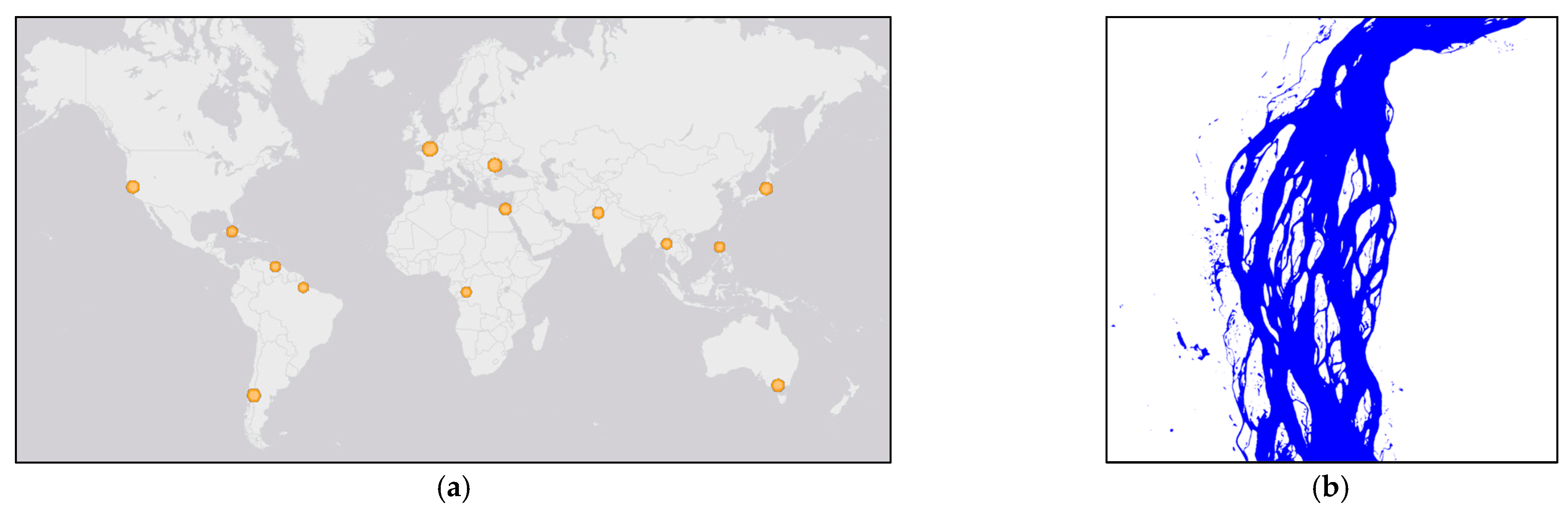
2.1. Study Areas and Period of Analysis

This study encompasses fourteen (14) areas within a 0.30° × 0.30° bounding box (Figure 2b). These areas include thirteen (13) rivers, seven lakes and reservoirs, and five paddy field areas.

The research covers wide-ranging locations globally (Figure 2a), with at least two representative area for each continent except Antarctica, to demonstrate consistency in satellite data fusion harmony irrespective of the geographic location. This approach allows us to analyze multiple surface water environments and evaluate the differences in inter-relatability across different types. The period of analysis is set to 2023, during which the operational periods of Landsat-8/9 (L8 and L9), Sentinel-2 (S2), and Sentinel-1 SAR (S1SAR) all intersect.

2.2. Surface Water Segmentation

The satellite images underwent standard pre-processing of optical and SAR data to produce the segmented, surface water images, as illustrated in Figure 3. These segmented images contain pixels classified as water, non-water, and contamination (e.g., cloud cover and cloud shadow), ensuring uniformity regardless of the satellite source for subsequent analyses.

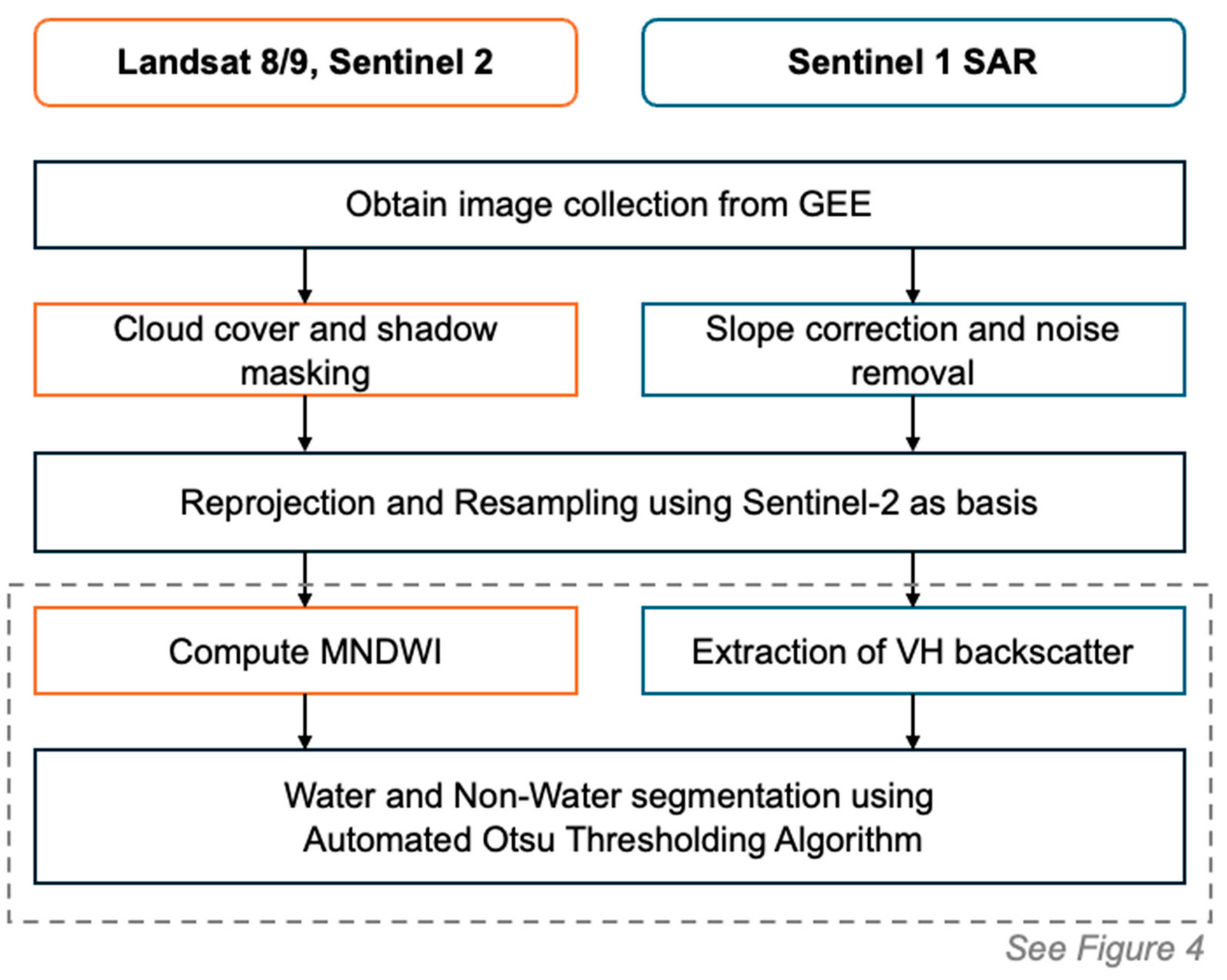
2.2.1. Satellite Data

The Google Earth Engine (GEE) platform was employed to access and process satellite data. Atmospherically corrected surface reflectances from the optical satellites were selected, as they are more suitable for quantitative remote sensing applications. These corrections account for atmospheric effects, providing a more accurate representation of the Earth’s surface [32,33].

Table 1. List of all satellite collections used in this study.

Satellite	Collection Name	GEE Image Collection Snippet
Landsat-8	Level 2, Collection 2, Tier 1	LANDSAT/LC08/C02/T1_L2
Landsat-9	Level 2, Collection 2, Tier 1	LANDSAT/LC09/C02/T1_L2
Sentinel-2	Multispectral Instrument Level-2A	COPERNICUS/S2_SR_HARMONIZED
	Cloud Probability	COPERNICUS/S2_CLOUD_PROBABILITY
Sentinel-1	C-band Synthetic Aperture Radar Ground-Range Detected	COPERNICUS/S1_GRD

details all the satellite scenes used in this study, along with the corresponding image collection names and data access snippets from GEE.

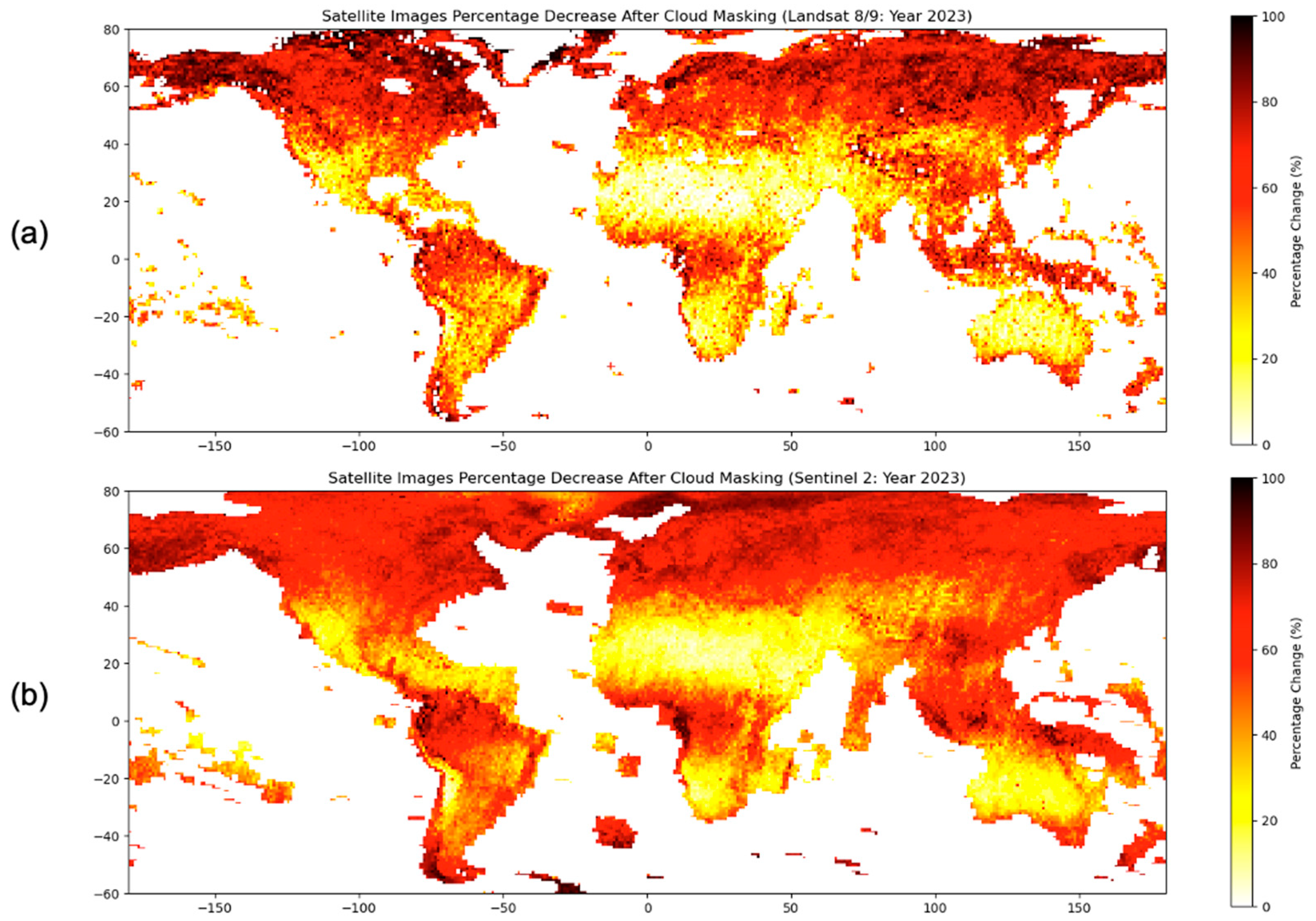
2.2.2. Cloud Cover and Cloud Shadow Masking

In this study, contaminations are defined as pixels identified as cloud covers, cloud shadows, and those with a medium to high probability of being cloud cover or cloud shadow. By removing pixels with medium to high probability of cloud cover and shadows, we ensure a more conservative approach minimizing misclassification as much as possible.

For Landsat 8/9 images, the Quality Assessment (QA) band, specifically the QA_PIXEL Bitmask, was used to mask these contaminations. In this bitmask, Bits 1, 3, and 4 correspond to dilated clouds, clouds, and cloud shadows, respectively. Dilated cloud pixels are expanded cloud pixels that account for potential uncertainties around the detected cloud. Additionally, Bits 8–9 for cloud confidence and Bits 10–11 for cloud shadow confidence were used to mask pixels with medium to high confidence of being cloud or cloud shadow.

For Sentinel-2 images, the Sentinel-2 Cloud Probability collection (see Table 1) was employed to assess cloud probability. Pixels with a cloud probability greater than 70% were masked and treated as contamination.

2.2.3. Resampling and Reprojection

Resampling and reprojection were applied to the satellite images to ensure uniformity in projection and spatial resolution across all datasets. Landsat 8/9 and Sentinel-1 SAR images were adjusted using Sentinel-2 as the reference. The satellites were reprojected to Sentinel-2 projection and resampled to a 10 m resolution. This approach maximizes the spatial resolution of the images for analysis. As a result, all satellite images in this study are aligned to the same projection and resolution.

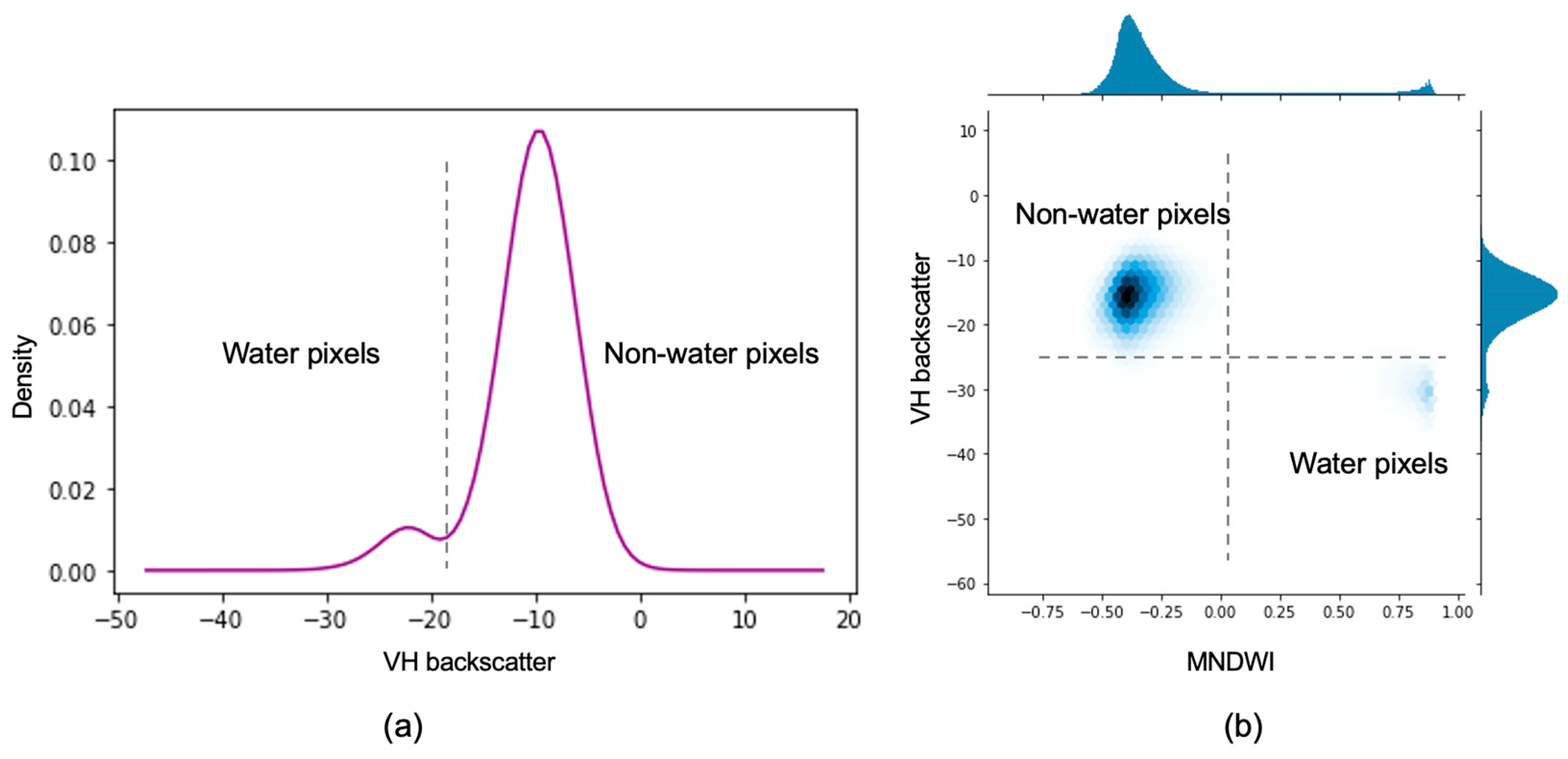
2.2.4. Surface Water Indexing: MNDWI

The modified normalized water index (MNDWI), which is a modification of the normalized water index because of its sensitivity to nearby built-up structures, was utilized for spectral indexing of optical satellites to address the complexities of various water bodies [34,35]. It has been widely applied in studies focused on segmenting surface water from non-water pixels [36,37]. The MNDWI formula, as in Equation (1), involves computing the spectral values of the green and shortwave infrared (SWIR) bands:

MNDWI = (Green − SWIR)/(Green + SWIR)

(1)

where the Green band has a wavelength between 530 and 590 nm (560 nm central wavelength for S2), and the SWIR band has a wavelength between 1570 and 1650 nm (1610 nm central wavelength for S2).

The dual-band cross-polarization VH backscatter of S1SAR was utilized for the delineation of surface water bodies. The backscatter coefficient is sensitive to soil moisture [38,39] providing valuable information about surface water. Furthermore, in vegetative environments, the double-bounce phenomena from VH backscatter are less affected by vegetation growth [40].

2.2.5. Image Segmentation through Automated Otsu Thresholding Algorithm

The Otsu algorithm facilitates image segmentation using a nonparametric and unsupervised approach, with the primary goal of satisfying two discriminant criteria over the pixel values: maximizing the between-class variance and minimizing the within-class variance [41].

In this study, water and non-water pixels were classified using the MNDWI layer for L8/9 and S2 and the VH backscatter coefficients for S1SAR. Fundamentally, higher MNDWI values indicate the presence of water due to the higher reflectance of water in the green band and its greater absorption in the SWIR band [42], which enhances the contrast between these bands. Conversely, lower VH backscatter values generally indicate water, as water surfaces reflect radar signals and lack the volume scattering caused by surface roughness [43]. Figure 4a illustrates the two distinct classes by showing the density distribution of VH polarization. The Otsu thresholding algorithm is then applied to determine the precise VH backscatter threshold that maximizes the between-class variance and minimizes the within-class variance, effectively separating water from non-water pixels. The same method will be used in the case of the MNDWI layer. The algorithm was applied automatically to each image in the time series across all study areas, enabling independent segmentation of each data source.

Given the distinct characteristics of MNDWI and VH backscatter coefficients, the automated Otsu thresholding approach provides an efficient and unbiased method for water segmentation across both optical and SAR imagery. The paired heatmaps in Figure 4b demonstrate that clear and consistent separation between water and non-water pixels can be achieved using this automated thresholding algorithm, whether applied to MNDWI from optical satellites or VH backscatter from SAR satellites.

While the thresholding approach used in this study is effective for binary water segmentation, it has certain limitations. This method is sufficient for demonstrating the feasibility of multi-satellite fusion, which is the primary objective of the study. However, challenges arise when the VH backscatter detects more than two land cover classes, resulting in inconsistent signals for water segmentation. Vegetation, in particular, can complicate the classification process, as it produces higher and more distinct backscatter values, creating a separate class from both surface water and non-cultivated fields, combined. This issue will be explored further in the following sections.

2.3. Performance Metrics: Kappa Coefficient as Degree of Harmony

In satellite remote sensing studies, acquiring ground truth data for validating satellite prediction is often impractical. However, the extensive application of remote sensing, especially optical satellites, in surface water detection over the decades has provided a high degree of confidence that these methods accurately reflect ground conditions. Therefore, in this study, we will not compare data against ground truth but will instead compare the independently segmented surface water images from different satellite sources to assess the feasibility of data fusion.

The kappa coefficient (κ) is a metric for evaluating the level of agreement between two mutually exclusive categorical models [44]. Unlike simple overall accuracy, the kappa coefficient adjusts for the agreement expected by chance, making it more robust in handling imbalanced datasets. This robustness is particularly advantageous in the context of surface water segmentation, where water pixels constitute a smaller portion of the entire image. By using the kappa coefficient, this study gains insights into the degree of harmony between two satellite sources. Consequently, describing the results using the ‘degree of harmony’ based on the kappa coefficient provides a more accurate interpretation from the comparative analysis between the satellite sources.

The formula for kappa coefficient, κ, derived from the confusion matrix is as follows:

κ = (P_o − P_e)/(1 − P_e)

(2)

The probability of observed agreement (P_o) is the relative agreement between the two satellites, and this formula is consistent with the formula of overall accuracy:

P_o = (TP + TN)/N

(3)

The hypothetical probability of chance agreement describes the proportion of times that the two satellites agree by chance or at random:

P_e = [(TP + FP)(TP + FN) + (TN + FP)(TN + FN)]/N²

(4)

where True Positives (TP) is the number of pixels where both satellite 1 and satellite 2 detected water; True Negatives (TN) is the number of pixels where both satellites detected non-water; False Positives (FP) is the number of pixels where one satellite detected water, but the other satellite detected non-water; False Negatives (FN) is the reverse of FP; and N is the total number of pixels in the image. In case of the presence of contaminations in the optical satellites, the contaminated pixels are ignored from the computations and subtracted from N.

Table 2. Interpretation of kappa coefficient in terms of degree of harmony between two satellites.

Kappa Coefficient, κ	Degree of Harmony Interpretation
1	Perfect Harmony
0.80–0.99	Very Strong Harmony
0.60–0.79	Strong Harmony
0.40–0.59	Moderate Harmony
0.20–0.39	Weak Harmony
0.01–0.19	Very Weak Harmony
≤0	No Harmony

summarizes the interpretation of kappa coefficient values in terms of the degree of harmony. A kappa value of 1 (κ = 1) indicates perfect harmony, meaning the two satellites can be used interchangeably or in combination for surface water detection. Conversely, a kappa value of 0 or less (κ ≤ 0) indicates no harmony, suggesting that the two satellites do not agree and should not be used interchangeably or in combination. Values of κ closer to 1 signify very strong harmony, while values closer to 0 denote very weak harmony. The degrees of harmony across three pairs of satellites (L9–S2, L9–S1, and S2–S1) will be discussed in the next section. Comparisons with L8 are excluded from the discussion because it consistently demonstrated near-perfect harmony with L9.

3. Results and Discussion

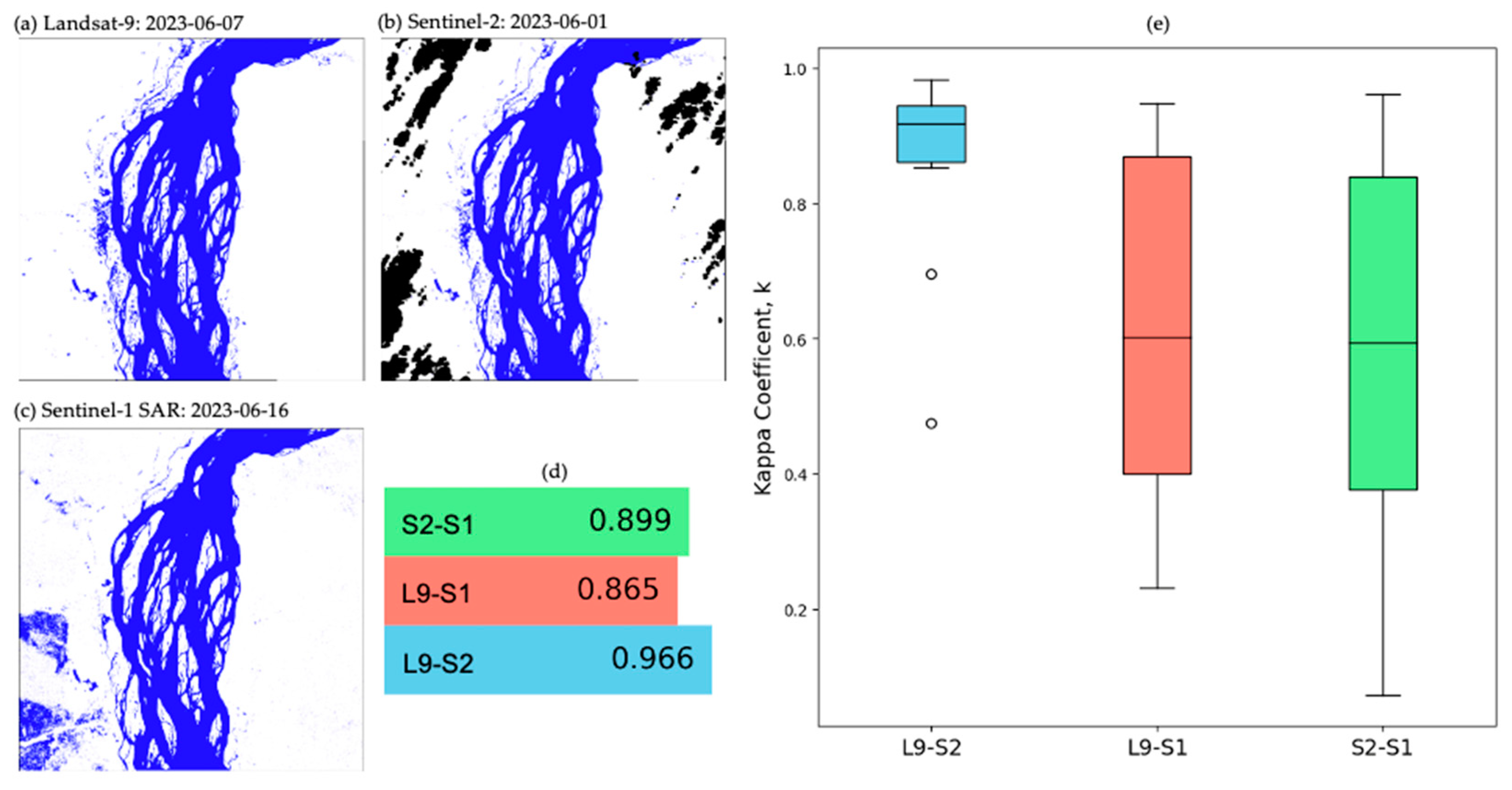
3.1. Satellite Harmony Performance: Study Areas

3.1.1. Across the Study Areas

The agreement between the different satellites sources was assessed across all representative images from the study areas. Figure 5a–c illustrate examples of segmented surface water images from the three satellites. Figure 5a displays a nearly pristine image, focusing on the river’s complexity with minimal to no contamination. Figure 5b shows the river with some contamination (a combination of cloud cover and cloud shadow) surrounding it. Figure 5c depicts the river along with additional detected water pixels in the lower right corner of the image. These images effectively illustrate the complexity of the clipped region of the Congo River. The kappa coefficients, shown in Figure 5d, indicate very strong harmony across all satellite pairs. The L9–S2 pair has near perfect harmony (κ = 0.966), while comparisons involving S1 (κ = 0.856, 0.899) still show very strong harmony. The observed differences in the images are likely due to a combination of satellite characteristics and variations in dates of capture.

Examining the overall kappa coefficients across all study areas in Figure 5e reveals that the harmony between L9 and S2 is very strong and consistent. Consequently, combining these optical satellites for surface water detection and analysis is highly recommended. In contrast, the kappa coefficients between either of the optical satellites (L9 or S2) and S1SAR exhibit significant variability. Some study areas show very weak to no harmony, while others indicate strong harmony. Although there are instances where the harmony is strong, the inconsistency makes the integration less straightforward. Therefore, caution should be exercised when combining Sentinel-1 with any of the other satellites.

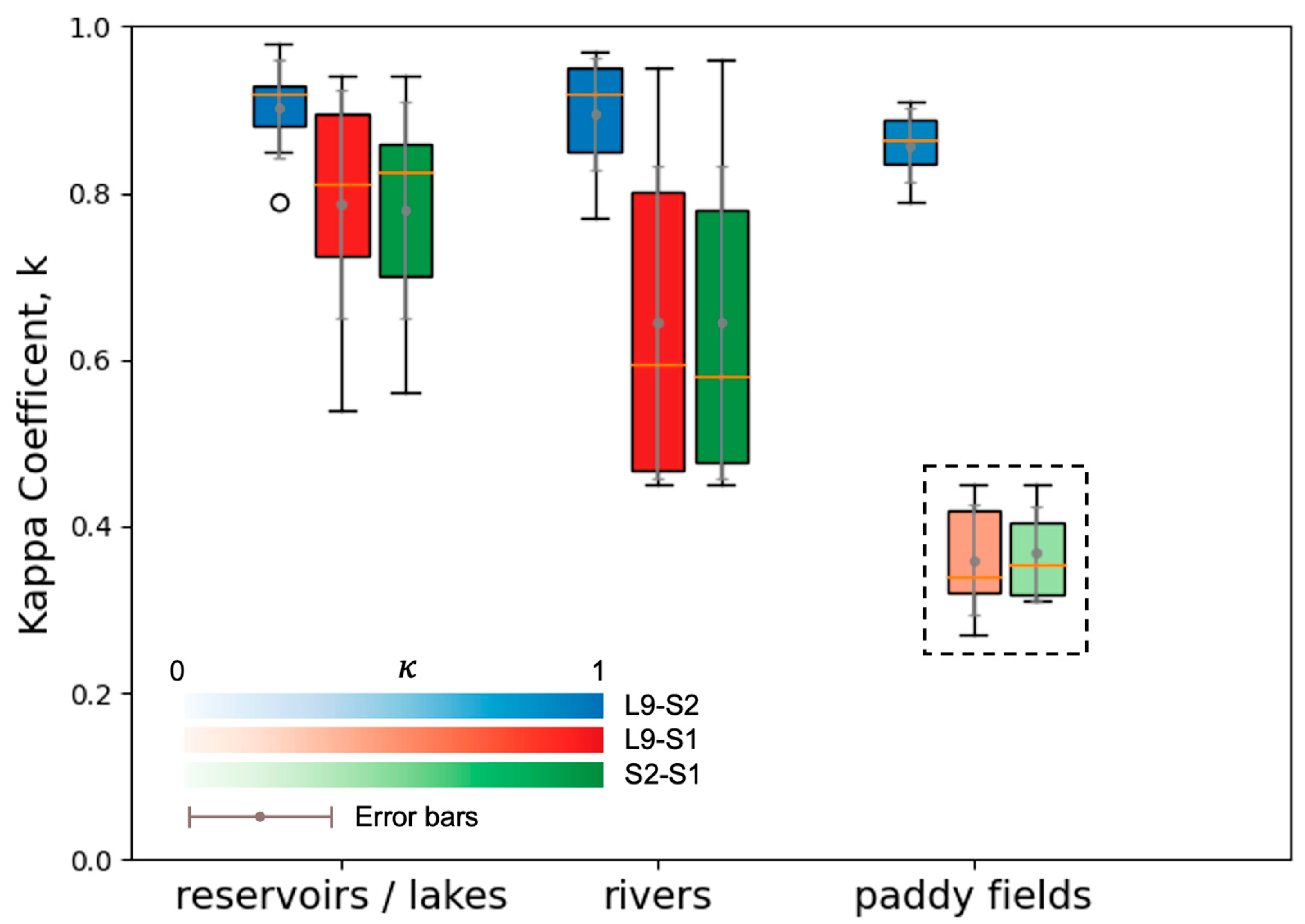
3.1.2. Across the Different Surface Water Environments

The degree of harmony resulting from optical and SAR satellite integration varies across different surface water environments. For stable water surfaces, such as lakes and reservoirs, the integration of optical and SAR observations is generally effective [45]. However, for rivers and their corresponding floodplains, this integration may be limited by water turbidity [46] and increased surface roughness caused by wind turbulence [47]. In paddy fields and other vegetative environments, challenges arise from the satellites’ differing abilities to detect water mixed with vegetation [48] and water underneath vegetation [49].

Therefore, it is crucial to closely evaluate how the degree of harmony in our study behaves when comparing different surface water bodies. The process involves multiple steps: If the surface water segmented image predominantly consists of one type of surface water body, the entire image is used. However, if the image includes multiple surface water types, smaller region-of-interest polygons are prepared to isolate each type. In the case of paddy fields, they are identified based on periods when the fields are observed to be flooded, a characteristic that distinguishes rice from other crops. For mixed types along rivers, such as those mixed with grasslands or paddy fields, the smaller regions of interest are considered as rivers only.

Figure 6 demonstrates that the strong harmony observed in Figure 5 persists across various surface water bodies. The integration of optical satellites (L9–S2, represented by blue boxplots) consistently exhibits very strong degrees of harmony, with κ values ranging from 0.80 to 0.98 and medians all above 0.85. The variability in the optical and SAR harmony is found to be primarily influenced by river and paddy field areas The values of κ in river areas varies from 0.45 to 0.97, showing moderate to very strong harmony. However, in paddy fields, the harmony is consistently weak, with κ values ranging from 0.27 to 0.45 and medians around 0.35 (see the enclosed dashed lines in Figure 6). This significant concern for data fusion stresses the challenges of detecting water in vegetative environments. From this study, we can draw two main recommendations: (1) we have strong confidence in integrating optical and SAR satellites for surface water detection across most environments (reservoirs, lakes, and rivers); (2) when detecting water in paddy fields and other vegetative environments, the confidence in integration remains low. Further studies are necessary to enhance our understanding and confidence in integrating satellites for applications involving detecting surface water in vegetations.

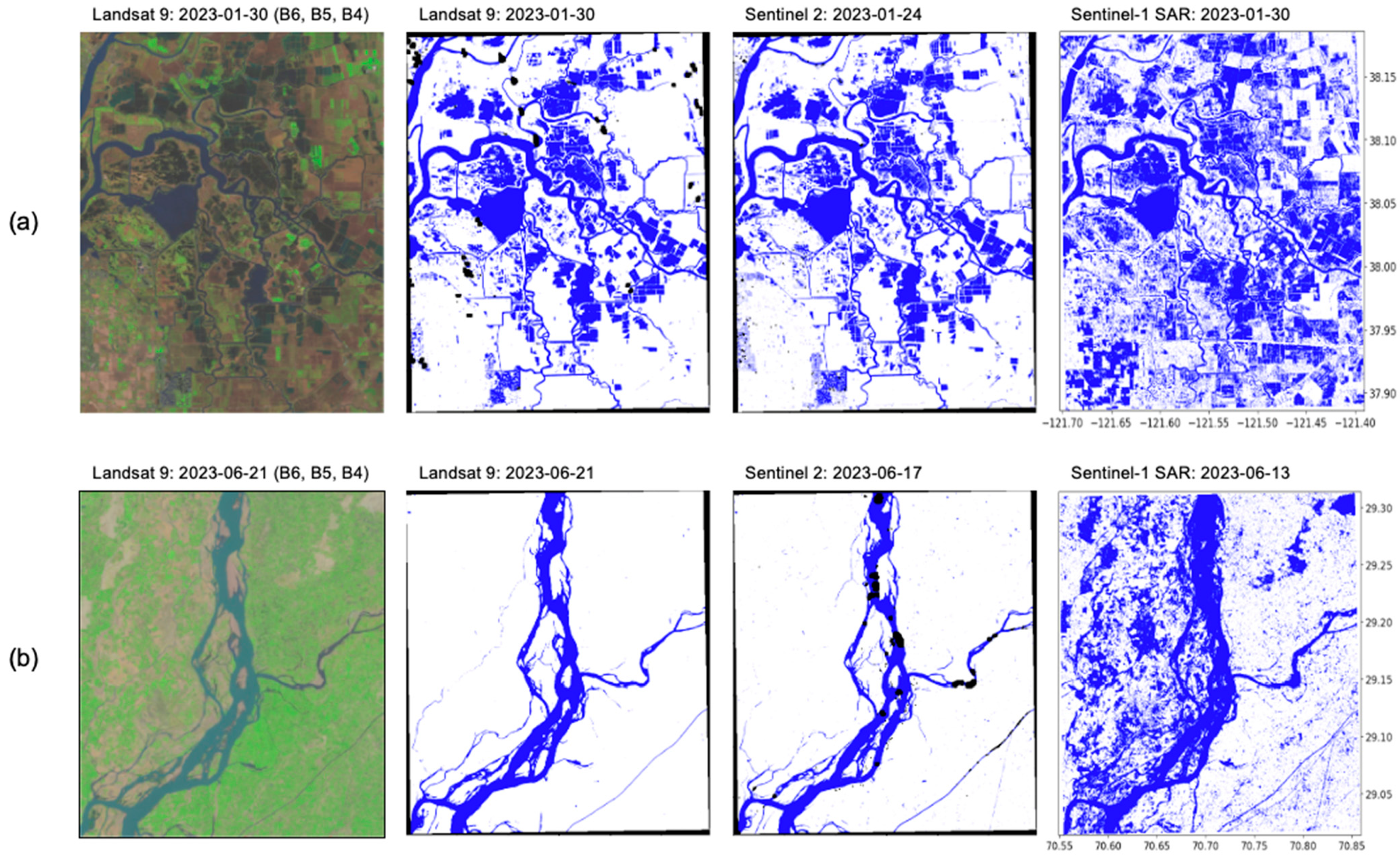
3.2. Limitations of the Automated Otsu Thresholding Algorithm: In the Presence of Vegetation

The automated Otsu thresholding algorithm is convenient and easily applicable to various satellite data sources by considering the MNDWI and VH backscatter values and their general behavior for water segmentation. However, the algorithm’s simplicity belies the complexity of real-world conditions, where values do not always perfectly segregate water and non-water pixels. Identifying scenarios where these limitations may arise is crucial. We will illustrate examples where the Otsu algorithm may be inappropriate, underscoring its potential shortcomings.

Examining the satellite imageries from two study area, Figure 7a (California, USA) and Figure 7b (Indus River, Pakistan), demonstrates how L9 and S2 effectively complement each other in detecting surface water particularly for rivers and open water from paddy field irrigation. The noise in surface water detection is clearly seen in the S1SAR images. By comparing the false-color images on the left with the S1SAR images, we can observe that vegetation presence causes misclassification. Combining bands 6 (shortwave infrared), 5 (near-infrared), and 4 (red) produces false-color images highlighting vegetation, land, and surface water areas. Vegetation generally manifests as surface or double-bounce backscattering, resulting in higher backscatter signals. These signals can be much higher than those from non-cultivated fields or water surfaces, leading to false segmentations, where vegetation is classified as non-water, while non-cultivated fields and water surfaces are classified as water pixels. This issue is particularly evident when closely examining the first images in both study areas, where non-cultivated fields or land pixels, shown in brown, are segmented as water in the respective SAR images.

While the simple binary Otsu thresholding algorithm is adequate for demonstrating the feasibility of multi-satellite data fusion in this study, exploring alternative approaches is highly recommended. Techniques such as multi-level thresholding [50,51], as well as unsupervised and supervised deep-learning methods [52,53], offer enhanced capabilities for water detection, particularly in more complex on-the-ground conditions.

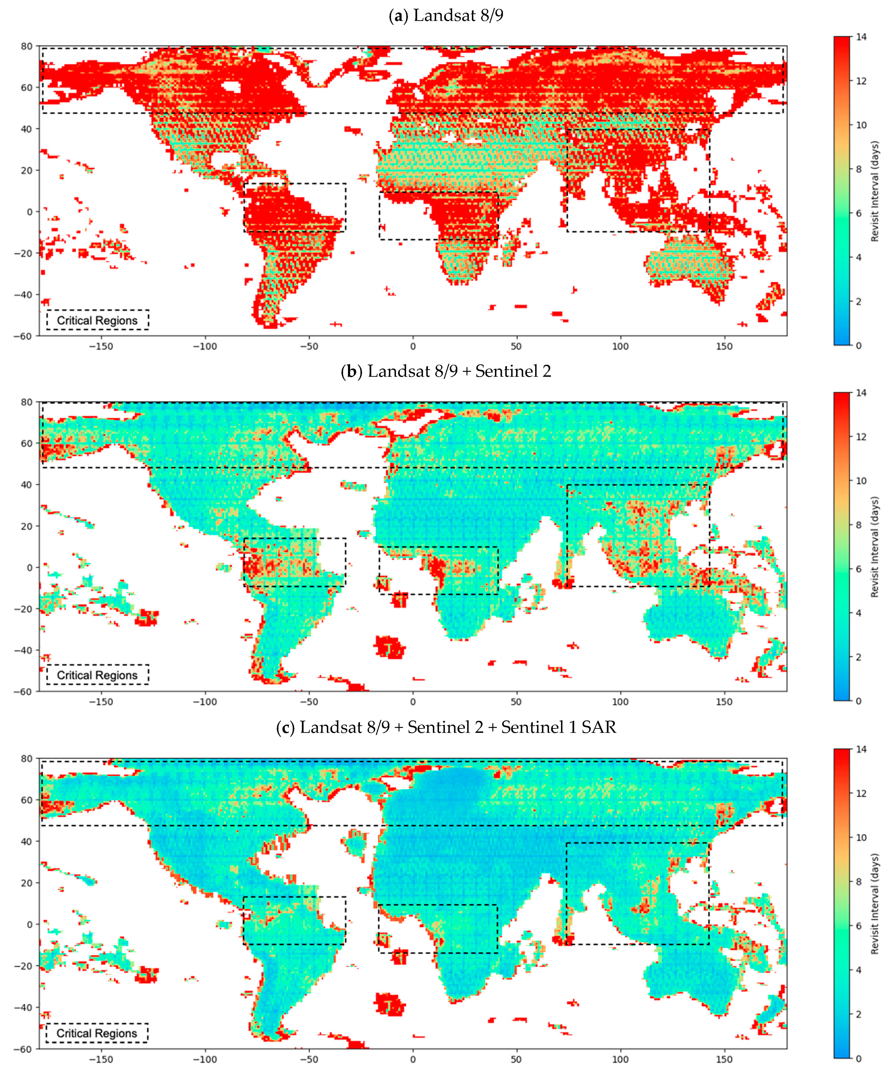
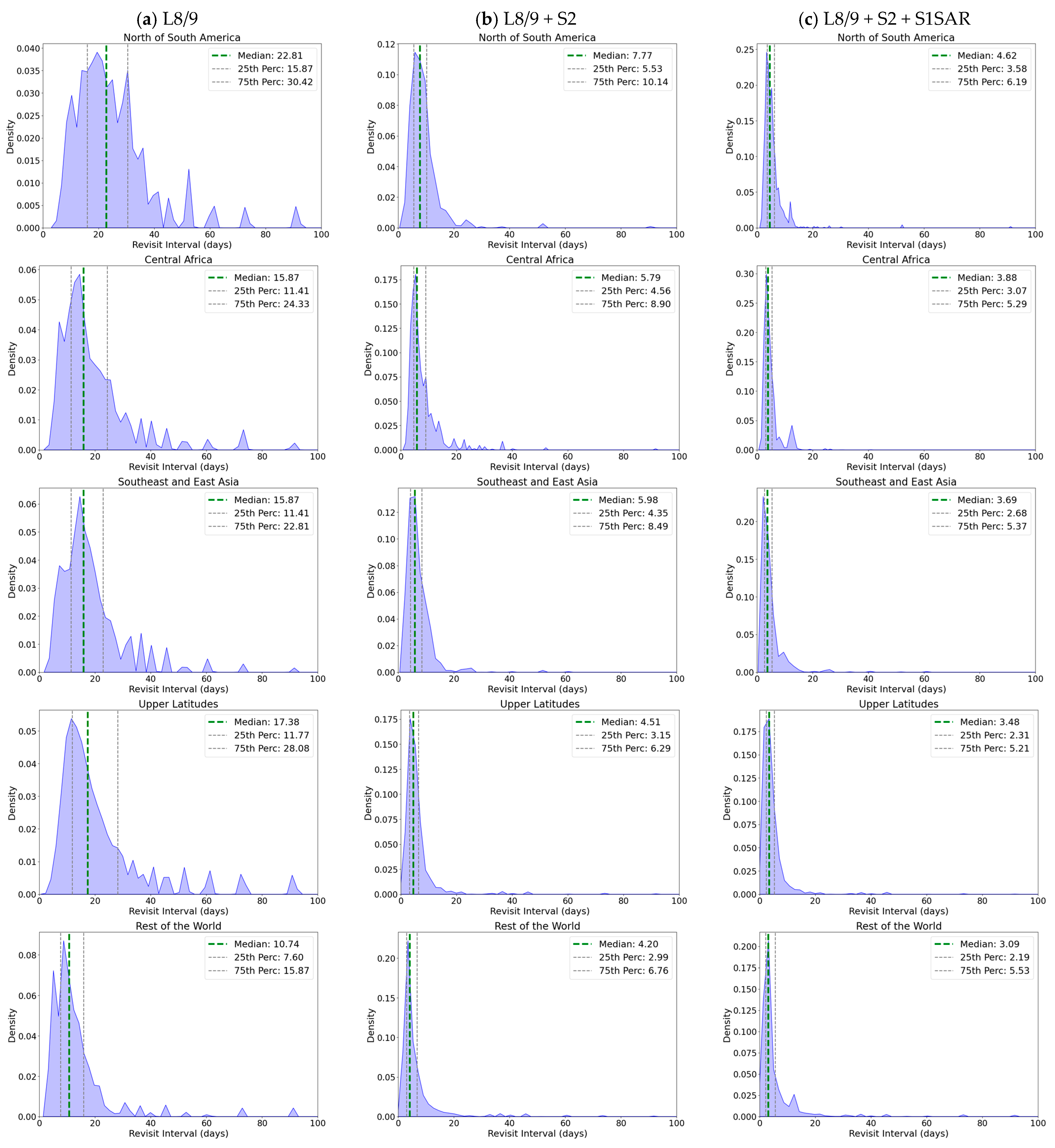
4. Global Revisit Interval

4.1. Progression after Data Fusion: Entire Year

The previous Sections provided insights into the potential and limitations of satellite data fusion. Overall, Landsat 8/9 and Sentinel-2 exhibit very strong harmony across all surface water environments, making the fusion of optical satellite data greatly recommended to enhance the density of surface water observations. Additionally, SAR data show strong harmony in reservoirs/lakes and rivers but present noticeable noise and highly variable harmony in vegetative environments such as paddy fields. Therefore, it is crucial to consider these limitations before integrating S1SAR satellite data for surface water detections.

The global revisit interval maps shown in Figure 8 were created by analyzing satellite imagery globally after cloud masking. For each pixel, the number of days with usable data was summed over the year and then divided by 365 to calculate the revisit interval. The maps illustrate the progression from using only Landsat 8/9 data to integrating optical data from both Landsat 8/9 and Sentinel-2 and finally incorporating SAR data. Each stage of this data fusion demonstrates significant improvements in revisit intervals. The most critical regions experiencing substantial reductions in usable observations after masking include northern South America, Central Africa, southeast and east Asia, and areas above 45 degrees latitude. When we zoom in on these regions, the improvements in revisit intervals become even more pronounced.

The progression of revisit intervals at each data fusion states (in Figure 9 and Figure 11) is assessed by extracting revisit interval values from the global maps for each critical region. Figure 9 offers additional insights, demonstrating how the revisit intervals improve in terms of median and interquartile range (IQR) as satellite data sources are integrated. The IQR gives an idea of the spread of the revisit interval values across different regions and fusion states. In critical regions, as shown in

Table 3. Median revisit intervals at the critical regions. Interquartile ranges (IQR) are in parentheses.

	L8/9 (Days)	L8/9 + S2 (Days)	L8/9 + S2 + S1SAR (Days)
North of South America	22.41	7.77	4.62
	(14.55)	(4.61)	(2.61)
Central Africa	15.87	5.79	3.88
	(12.92)	(4.34)	(2.22)
Southeast and East Asia	15.87	5.98	3.69
	(11.40)	(4.14)	(2.69)
Upper Latitudes	17.38	4.51	3.48
	(16.31)	(3.14)	(2.90)
Rest of the World	10.74	4.20	3.09
	(8.27)	(3.77)	(3.34)

Rest of the World are all the regions besides the critical regions.

, the median revisit interval ranges from 15.87 to 22.81 days (IQR: 14.41–30.42 days) when using Landsat imagery alone. This interval improves to a median of 4.51 to 7.77 days (IQR: 3.15–10.14 days) after incorporating Sentinel-2 and further improves to a median of 3.48 to 4.62 days (IQR: 2.31–6.19 days) after integrating Sentinel-1 SAR data. These values underscore the enhanced monitoring capability provided by multi-satellite fusion, particularly in critical regions where the median revisit intervals significantly decrease and the IQR narrows, indicating that revisit interval values are becoming more centered around the median. As anticipated, the revisit interval values for the rest of the world are significantly better than those of the critical regions.

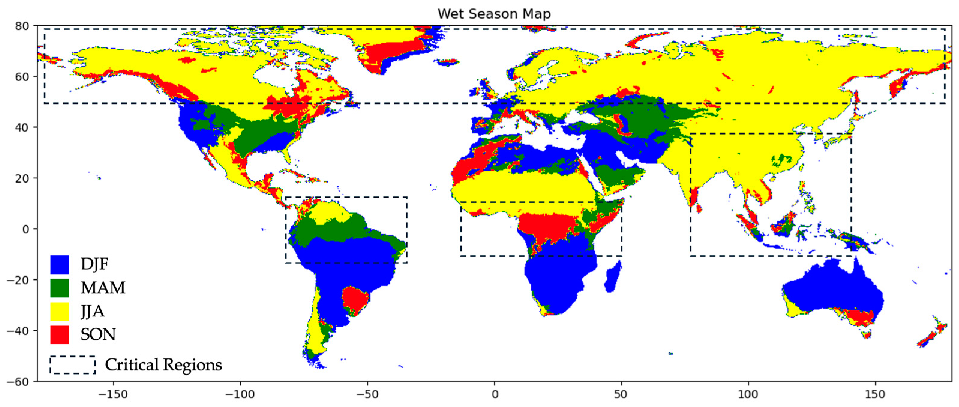
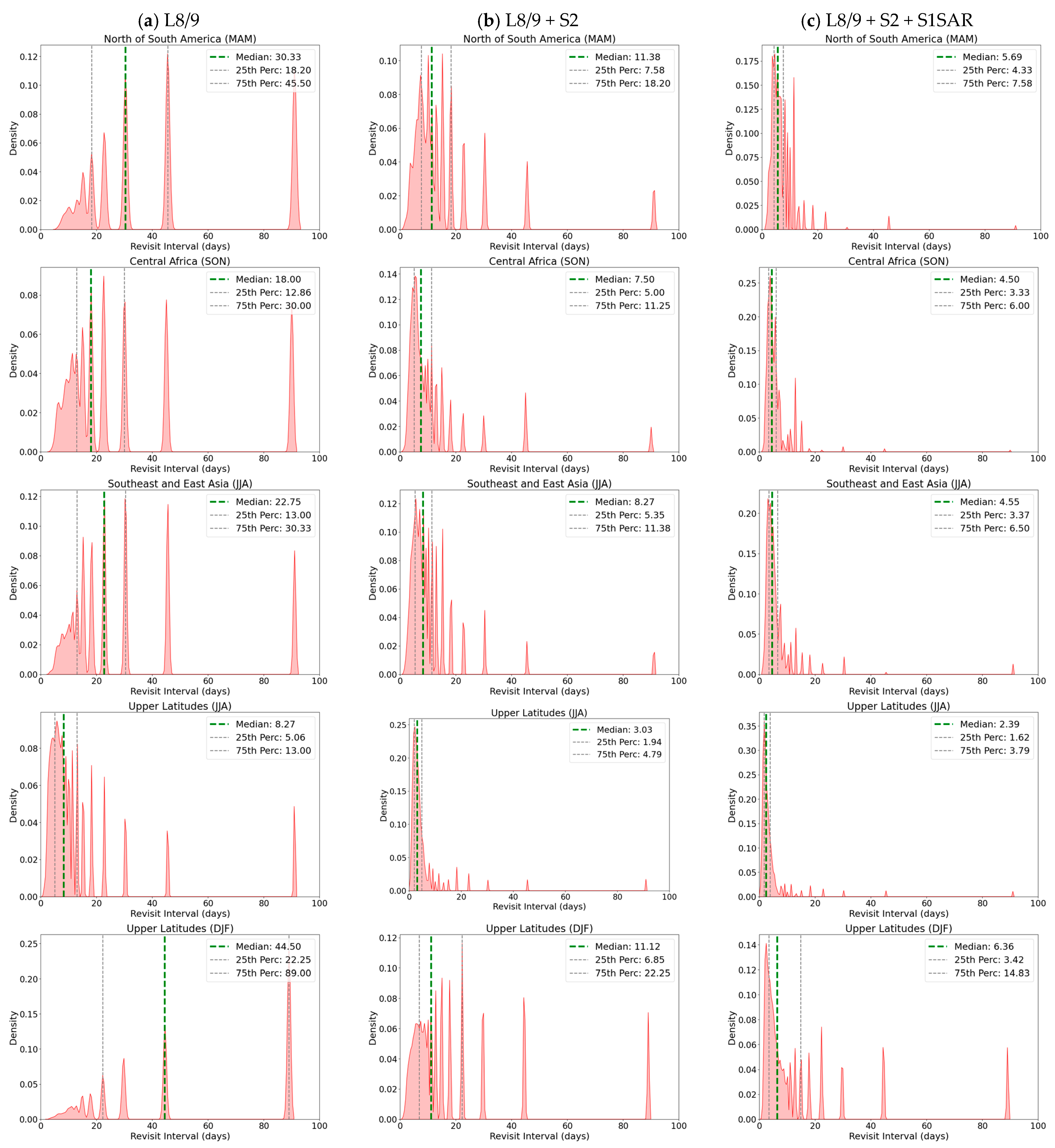
4.2. Progression after Data Fusion: Wet Season Months

Revisit intervals are significantly influenced by cloud cover, particularly during the rainy season when the number of cloudy days increases. Therefore, it is crucial to examine the trend and progression of revisit intervals from data fusion in critical regions during their respective wet season months. To realize this, identifying the wet season months is essential. The monthly aggregates from the ERA-5 Land dataset [54], produced by the European Centre for Medium-Range Weather Forecasts (ECMWF), were used for this purpose. Utilizing 30 years of monthly precipitation data (1994–2023), we created a wet season map, shown in Figure 9. Seasons are grouped into three consecutive months: December to February (DJF), March to May (MAM), June to August (JJA), and September to November (SON). The mean total precipitation for each season was calculated and compared. The wet season months is the set of three consecutive months with the highest mean total precipitation.

The wet season map in Figure 10 visually identifies the dominant wet season months for each region. In regions exhibiting mixed trends, the central trend will be selected as the dominant wet season months for analysis, as shown in

Table 4. Dominant wet season months at each critical region for revisit interval analysis.

Critical Regions	Dominant Wet Season Months	Dominant Wet Season Months for Analysis
North of South America	DJF, MAM	MAM
Central Africa	DJF, JJA, SON	SON
Southeast and East Asia	JJA	JJA
Upper Latitudes	JJA	JJA

. This approach ensures a consistent basis for evaluating the data fusion of revisit intervals in the critical regions.

When examining the revisit interval during the wet season months, Figure 11 and

Table 5. Median revisit intervals at the critical regions during the wet season months. Interquartile ranges (IQR) are in parentheses.

	L8/9 (Days)	L8/9 + S2 (Days)	L8/9 + S2 + S1SAR (Days)
North of South America (MAM)	30.33 (27.30)	11.38 (10.62)	5.69 (3.25)
Central Africa (SON)	18.00 (17.14)	7.50 (6.25)	4.50 (2.67)
Southeast and East Asia (JJA)	22.75 (17.33)	8.27 (6.03)	4.55 (3.13)
Upper Latitudes (JJA)	8.27 (7.94)	3.03 (2.85)	2.39 (2.17)
Upper Latitudes (DFJ)	44.50 (66.75)	11.12 (15.40)	6.36 (11.41)

reveal significant increases in median revisit intervals and interquartile ranges across critical regions for all data fusion states. Outlier values are more pronounced until the integration of optical data, and it is only after the inclusion of S1SAR that the distribution shape begins to resemble the revisit interval density distribution observed in Figure 8. Figure 12 illustrates the percentage change in revisit intervals from year-round to wet season months, showing an increase in the median revisit interval ranging from 13.42% to 43.35% across different critical regions and fusion states. The IQR exhibits an even larger percentage increase, from 16.36% to 130.37%. These findings provide better insights and more realistic expectations for revisit intervals during the rainy season, a period when denser observation of surface water dynamics is crucial.

The trend in these metrics for Upper Latitudes differs from the expectations established for the first three critical regions. During the wet season months of June, July, and August (JJA), the Upper Latitudes showed notable improvements in both median RI and IQR (represented in shades of blue). The median RI decreased by 31.32% to 52.53%, while the IQR decreased by 3.50% to 49.29% across the fusion states. This behavior aligns with observations by [55], which attribute it to the summer solstice occurring in the third week of June. Optical satellites, which rely on the sun as their energy source, operate sun-synchronously. During the summer solstice and months prior and after, daylight can extend up to 24 h per day in the northern hemisphere, significantly increasing satellite revisit frequencies and swath overlaps in the Upper Latitudes. Conversely, during the winter solstice (occurring around the third week of December) and months prior and after, when there is almost no daylight for months, the availability of useful satellite information worsens dramatically. For the months of December, January, and February (DJF), the median RI increases by approximately 82.76 to 156.04%, and the IQR expands almost three to four times. This indicates that, aside from cloud cover and shadow contamination, the tilt of the Earth relative to the sun profoundly affects the amount of useful observations from optical satellites, especially in the Upper Latitudes up to the polar regions.

5. Conclusions

This research established the feasibility of the data fusion of different high-resolution open-source satellites for enhancing surface water monitoring. We explored the potential and limitations of integrating multiple satellite sources in producing high temporal and high spatial surface water observations. Moreover, we presented more realistic expectations of global revisit intervals considering the following: (1) cloud cover and cloud shadow masking, (2) progressive satellite fusion states, (3) global and critical regions, (4) whole year and wet season months. We also recommended future studies to improve the harmony between optical and SAR satellites across different surface water environments.

Our findings indicate that optical satellites—Landsat 8/9 (L8/9) and Sentinel-2 (S2)—exhibit very strong harmony across all surface water environments. Therefore, combining these optical satellites to produce consistent surface water extent images is greatly recommended. The degree of harmony between optical satellites and Sentinel-1 SAR (S1SAR) is weak. Generally, with S1SAR, the degree of harmony is strong for reservoirs/lakes and river environments but relatively weak for detecting water in vegetative environments such as paddy fields. This variability in water detection may be attributed to the limitations of the binary Otsu thresholding algorithm used in the study. Based on these findings, we recommend the following:

• Explore alternative thresholding techniques: Preferably, multi-level thresholding that considers the different behaviors of various land covers;
• Investigate the complexity of vegetative environments: Examine the relationships between surface reflectances, water indices, vegetation indices, and radar backscatter signals to aid in integrating optical and SAR satellites.

Additionally, the revisit interval maps illustrated the distribution of available surface water observations. Over the year, we observed that integrating the optical satellites significantly increases the density of observations up to threefold, especially in critical regions. Furthermore, integrating SAR satellite observations ensures representative observations during the rainy season, with intervals of at least every 12 days. In comparison to existing surface water datasets, our approach offers the promise of both high spatial and temporal resolution (see Figure 13), featuring a 10-meter spatial resolution and a sub-weekly temporal resolution. The median revisit intervals range from 3.09 to 4.62 days for annual analysis, and from 2.36 to 6.36 days during the rainy season, providing a more granular and timely assessment of surface water dynamics.

With high temporal and spatial resolution, monitoring rapid changes in reservoirs, rivers, and floodplains during extreme rainfall events becomes highly effective. As satellite observations are increasingly validated against real-world ground truth through techniques such as spectral indexing and machine learning, their applications continue to expand. We can leverage this rich dataset to model surface water dynamics at high temporal resolutions, maximizing the utility of satellite observations for detailed and timely analysis.

Furthermore, as new satellite missions (e.g., SWOT and Landsat Next) are launched, it will be essential to study the integration suitability and, consequently, the combined global revisit intervals, of these sources when they come into orbit. Improving the fusion of all these open-source satellites at present and in the future will be integral to the further promotion of the application of Earth observations satellites to studies requiring more frequent satellite observations, such as flood and inundation studies and hydrological modeling.

References

1. Gangrade, S.; Lu, D.; Kao, S.; Painter, S.L. Machine Learning Assisted Reservoir Operation Model for Long-Term Water Management Simulation. JAWRA J. Am. Water Resour. Assoc. 2022, 58, 1592–1603. [Google Scholar] [CrossRef]
2. Donchyts, G.; Winsemius, H.; Baart, F.; Dahm, R.; Schellekens, J.; Gorelick, N.; Iceland, C.; Schmeier, S. High-Resolution Surface Water Dynamics in Earth’s Small and Medium-Sized Reservoirs. Sci. Rep. 2022, 12, 13776. [Google Scholar] [CrossRef] [PubMed]
3. Lane, S.N. Natural Flood Management. WIREs Water 2017, 4, e1211. [Google Scholar] [CrossRef]
4. Morita, M. Quantification of Increased Flood Risk Due to Global Climate Change for Urban River Management Planning. Water Sci. Technol. 2011, 63, 2967–2974. [Google Scholar] [CrossRef] [PubMed]
5. Rezanezhad, F.; McCarter, C.P.R.; Lennartz, B. Editorial: Wetland Biogeochemistry: Response to Environmental Change. Front. Environ. Sci. 2020, 8, 55. [Google Scholar] [CrossRef]
6. Meijide, A.; Gruening, C.; Goded, I.; Seufert, G.; Cescatti, A. Water Management Reduces Greenhouse Gas Emissions in a Mediterranean Rice Paddy Field. Agric. Ecosyst. Environ. 2017, 238, 168–178. [Google Scholar] [CrossRef]
7. Karpatne, A.; Khandelwal, A.; Chen, X.; Mithal, V.; Faghmous, J.; Kumar, V. Global Monitoring of Inland Water Dynamics: State-of-the-Art, Challenges, and Opportunities. Comput. Sustain. 2016, 645, 121–147. [Google Scholar]
8. Wulder, M.A.; Roy, D.P.; Radeloff, V.C.; Loveland, T.R.; Anderson, M.C.; Johnson, D.M.; Healey, S.; Zhu, Z.; Scambos, T.A.; Pahlevan, N.; et al. Fifty Years of Landsat Science and Impacts. Remote Sens. Environ. 2022, 280, 113195. [Google Scholar] [CrossRef]
9. Melton, F.S.; Huntington, J.; Grimm, R.; Herring, J.; Hall, M.; Rollison, D.; Erickson, T.; Allen, R.; Anderson, M.; Fisher, J.B.; et al. OpenET: Filling a Critical Data Gap in Water Management for the Western United States. JAWRA J. Am. Water Resour. Assoc. 2022, 58, 971–994. [Google Scholar] [CrossRef]
10. Buma, W.G.; Lee, S.-I.; Seo, J.Y. Recent Surface Water Extent of Lake Chad from Multispectral Sensors and GRACE. Sensors 2018, 18, 2082. [Google Scholar] [CrossRef]
11. Hansen, M.C.; Potapov, P.V.; Pickens, A.H.; Tyukavina, A.; Hernandez-Serna, A.; Zalles, V.; Turubanova, S.; Kommareddy, I.; Stehman, S.V.; Song, X.-P.; et al. Global Land Use Extent and Dispersion within Natural Land Cover Using Landsat Data. Environ. Res. Lett. 2022, 17, 034050. [Google Scholar] [CrossRef]
12. Pekel, J.-F.; Cottam, A.; Gorelick, N.; Belward, A.S. High-Resolution Mapping of Global Surface Water and Its Long-Term Changes. Nature 2016, 540, 418–422. [Google Scholar] [CrossRef]
13. Pickens, A.H.; Hansen, M.C.; Hancher, M.; Stehman, S.V.; Tyukavina, A.; Potapov, P.; Marroquin, B.; Sherani, Z. Mapping and Sampling to Characterize Global Inland Water Dynamics from 1999 to 2018 with Full Landsat Time-Series. Remote Sens. Environ. 2020, 243, 111792. [Google Scholar] [CrossRef]
14. Tulbure, M.G.; Broich, M.; Stehman, S.V.; Kommareddy, A. Surface Water Extent Dynamics from Three Decades of Seasonally Continuous Landsat Time Series at Subcontinental Scale in a Semi-Arid Region. Remote Sens. Environ. 2016, 178, 142–157. [Google Scholar] [CrossRef]
15. Mueller, N.; Lewis, A.; Roberts, D.; Ring, S.; Melrose, R.; Sixsmith, J.; Lymburner, L.; McIntyre, A.; Tan, P.; Curnow, S.; et al. Water Observations from Space: Mapping Surface Water from 25 Years of Landsat Imagery across Australia. Remote Sens. Environ. 2016, 174, 341–352. [Google Scholar] [CrossRef]
16. Yamazaki, D.; Trigg, M.A.; Ikeshima, D. Development of a Global ~90m Water Body Map Using Multi-Temporal Landsat Images. Remote Sens. Environ. 2015, 171, 337–351. [Google Scholar] [CrossRef]
17. Malenovský, Z.; Rott, H.; Cihlar, J.; Schaepman, M.E.; García-Santos, G.; Fernandes, R.; Berger, M. Sentinels for Science: Potential of Sentinel-1,-2, and-3 Missions for Scientific Observations of Ocean, Cryosphere, and Land. Remote Sens. Environ. 2012, 120, 91–101. [Google Scholar] [CrossRef]
18. Berger, M.; Moreno, J.; Johannessen, J.A.; Levelt, P.F.; Hanssen, R.F. ESA’s Sentinel Missions in Support of Earth System Science. Remote Sens. Environ. 2012, 120, 84–90. [Google Scholar] [CrossRef]
19. Mandanici, E.; Bitelli, G. Preliminary Comparison of Sentinel-2 and Landsat 8 Imagery for a Combined Use. Remote Sens. 2016, 8, 1014. [Google Scholar] [CrossRef]
20. Claverie, M.; Ju, J.; Masek, J.G.; Dungan, J.L.; Vermote, E.F.; Roger, J.-C.; Skakun, S.V.; Justice, C. The Harmonized Landsat and Sentinel-2 Surface Reflectance Data Set. Remote Sens. Environ. 2018, 219, 145–161. [Google Scholar] [CrossRef]
21. Tulbure, M.; Broich, M.; Gaines, M.; Stehman, S.; Pavelsky, T.; Perin, V.; Ju, J.; Yin, S.; Mai, J.; Betbeder-Matibet, L. Towards Global Flood Mapping with Machine Learning Based on the Harmonized Landsat-Sentinel 2 Data. In Proceedings of the AGU Fall Meeting Abstracts, New Orleans, LA, USA, 13–17 December 2021; Volume 2021, p. H44E-03. [Google Scholar]
22. Tulbure, M.G.; Broich, M.; Ju, J.; Masek, J.G.; Wearne, J. Quantifying Surface Water Extent and Flooding in a Dynamic Dryland River System Using the Harmonized Landsat/Sentinel-2 Reflectance Product. In Proceedings of the AGU Fall Meeting Abstracts, Washington, DC, USA, 10–14 December 2018; Volume 2018, p. H21E-08. [Google Scholar]
23. Ju, Y.; Bohrer, G. Classification of Wetland Vegetation Based on NDVI Time Series from the HLS Dataset. Remote Sens. 2022, 14, 2107. [Google Scholar] [CrossRef]
24. Hu, J.; Chen, Y.; Cai, Z.; Wei, H.; Zhang, X.; Zhou, W.; Wang, C.; You, L.; Xu, B. Mapping Diverse Paddy Rice Cropping Patterns in South China Using Harmonized Landsat and Sentinel-2 Data. Remote Sens. 2023, 15, 1034. [Google Scholar] [CrossRef]
25. Li, J.; Li, L.; Song, Y.; Chen, J.; Wang, Z.; Bao, Y.; Zhang, W.; Meng, L. A Robust Large-Scale Surface Water Mapping Framework with High Spatiotemporal Resolution Based on the Fusion of Multi-Source Remote Sensing Data. Int. J. Appl. Earth Obs. Geoinf. 2023, 118, 103288. [Google Scholar] [CrossRef]
26. Valerio, F.; Godinho, S.; Ferraz, G.; Pita, R.; Gameiro, J.; Silva, B.; Marques, A.T.; Silva, J.P. Multi-Temporal Remote Sensing of Inland Surface Waters: A Fusion of Sentinel-1 & 2 Data Applied to Small Seasonal Ponds in Semiarid Environments. bioRxiv 2024. [Google Scholar] [CrossRef]
27. Liu, Q.; Zhang, S.; Wang, N.; Ming, Y.; Huang, C. Fusing Landsat-8, Sentinel-1, and Sentinel-2 Data for River Water Mapping Using Multidimensional Weighted Fusion Method. IEEE Trans. Geosci. Remote Sens. 2022, 60, 4208012. [Google Scholar] [CrossRef]
28. Tang, H.; Lu, S.; Ali Baig, M.H.; Li, M.; Fang, C.; Wang, Y. Large-Scale Surface Water Mapping Based on Landsat and Sentinel-1 Images. Water 2022, 14, 1454. [Google Scholar] [CrossRef]
29. Li, J.; Roy, D. A Global Analysis of Sentinel-2A, Sentinel-2B and Landsat-8 Data Revisit Intervals and Implications for Terrestrial Monitoring. Remote Sens. 2017, 9, 902. [Google Scholar] [CrossRef]
30. Liu, Y.; Liu, R.; Shang, R. GLOBMAP SWF: A Global Annual Surface Water Cover Frequency Dataset during 2000–2020. Earth Syst. Sci. Data 2022, 14, 4505–4523. [Google Scholar] [CrossRef]
31. Han, Q.; Niu, Z. Construction of the Long-Term Global Surface Water Extent Dataset Based on Water-NDVI Spatio-Temporal Parameter Set. Remote Sens. 2020, 12, 2675. [Google Scholar] [CrossRef]
32. Baba, H.; Kannemadugu, S.; Hareef Baba, K.; Joshi, A.K.; Moharil, S. V Surface Reflectance Retrieval from the High Resolution Multispectral Satellite Image Using 6S Radiative Transfer Model. Int. J. Remote Sens. GIS 2013, 2, 1–9. [Google Scholar]
33. Chen, H.-W.; Cheng, K.-S. A Conceptual Model of Surface Reflectance Estimation for Satellite Remote Sensing Images Using in Situ Reference Data. Remote Sens. 2012, 4, 934–949. [Google Scholar] [CrossRef]
34. Singh, K.V.; Setia, R.; Sahoo, S.; Prasad, A.; Pateriya, B. Evaluation of NDWI and MNDWI for Assessment of Waterlogging by Integrating Digital Elevation Model and Groundwater Level. Geocarto Int. 2015, 30, 650–661. [Google Scholar] [CrossRef]
35. Ali, M.I.; Dirawan, G.D.; Hasim, A.H.; Abidin, M.R. Detection of Changes in Surface Water Bodies Urban Area with NDWI and MNDWI Methods. Int. J. Adv. Sci. Eng. Inf. Technol. 2019, 9, 946–951. [Google Scholar] [CrossRef]
36. Laonamsai, J.; Julphunthong, P.; Saprathet, T.; Kimmany, B.; Ganchanasuragit, T.; Chomcheawchan, P.; Tomun, N. Utilizing NDWI, MNDWI, SAVI, WRI, and AWEI for Estimating Erosion and Deposition in Ping River in Thailand. Hydrology 2023, 10, 70. [Google Scholar] [CrossRef]
37. da Silva, J.L.B.; de Albuquerque Moura, G.B.; da Silva, M.V.; Lopes, P.M.O.; de Souza Guedes, R.V.; de França e Silva, Ê.F.; Ortiz, P.F.S.; de Moraes Rodrigues, J.A. Changes in the Water Resources, Soil Use and Spatial Dynamics of Caatinga Vegetation Cover over Semiarid Region of the Brazilian Northeast. Remote Sens. Appl. 2020, 20, 100372. [Google Scholar] [CrossRef]
38. Vreugdenhil, M.; Wagner, W.; Bauer-Marschallinger, B.; Pfeil, I.; Teubner, I.; Rüdiger, C.; Strauss, P. Sensitivity of Sentinel-1 Backscatter to Vegetation Dynamics: An Austrian Case Study. Remote Sens. 2018, 10, 1396. [Google Scholar] [CrossRef]
39. Huang, S.; Ding, J.; Zou, J.; Liu, B.; Zhang, J.; Chen, W. Soil Moisture Retrival Based on Sentinel-1 Imagery under Sparse Vegetation Coverage. Sensors 2019, 19, 589. [Google Scholar] [CrossRef]
40. Tran, K.H.; Menenti, M.; Jia, L. Surface Water Mapping and Flood Monitoring in the Mekong Delta Using Sentinel-1 SAR Time Series and Otsu Threshold. Remote Sens. 2022, 14, 5721. [Google Scholar] [CrossRef]
41. Otsu, N. A Threshold Selection Method from Gray-Level Histograms. Automatica 1975, 11, 23–27. [Google Scholar] [CrossRef]
42. Xu, H. Modification of Normalised Difference Water Index (NDWI) to Enhance Open Water Features in Remotely Sensed Imagery. Int. J. Remote Sens. 2006, 27, 3025–3033. [Google Scholar] [CrossRef]
43. Roth, F.; Tupas, M.E.; Bauer-Marschallinger, B.; Wagner, W. Comparison of VV and VH Polarization for Sentinel-1 Based Flood Mapping. In Proceedings of the Hydrospace 2023, Lissabon, Portugal, 27 November–1 December 2023. [Google Scholar]
44. Altman, D.G. Practical Statistics for Medical Research; Chapman and Hall/CRC: Boca Raton, FL, USA, 1990; ISBN 9780429258589. [Google Scholar]
45. Peña-Luque, S.; Ferrant, S.; Cordeiro, M.C.R.; Ledauphin, T.; Maxant, J.; Martinez, J.-M. Sentinel-1 & 2 Multitemporal Water Surface Detection Accuracies, Evaluated at Regional and Reservoirs Level. Remote Sens. 2021, 13, 3279. [Google Scholar] [CrossRef]
46. Schmitt, M. Potential of Large-Scale Inland Water Body Mapping from Sentinel-1/2 Data on the Example of Bavaria’s Lakes and Rivers. PFG—J. Photogramm. Remote Sens. Geoinf. Sci. 2020, 88, 271–289. [Google Scholar] [CrossRef]
47. Dewan, A.M.; Kankam-Yeboah, K.; Nishigaki, M. Using Synthetic Aperture Radar (SAR) Data for Mapping River Water Flooding in an Urban Landscape: A Case Study of Greater Dhaka, Bangladesh. J. Jpn. Soc. Hydrol. Water Resour. 2006, 19, 44–54. [Google Scholar] [CrossRef]
48. Druce, D.; Tong, X.; Lei, X.; Guo, T.; Kittel, C.M.M.; Grogan, K.; Tottrup, C. An Optical and SAR Based Fusion Approach for Mapping Surface Water Dynamics over Mainland China. Remote Sens. 2021, 13, 1663. [Google Scholar] [CrossRef]
49. Dunn, B.; Ai, E.; Alger, M.J.; Fanson, B.; Fickas, K.C.; Krause, C.E.; Lymburner, L.; Nanson, R.; Papas, P.; Ronan, M.; et al. Wetlands Insight Tool: Characterising the Surface Water and Vegetation Cover Dynamics of Individual Wetlands Using Multidecadal Landsat Satellite Data. Wetlands 2023, 43, 37. [Google Scholar] [CrossRef]
50. Rahaman, J.; Sing, M. An Efficient Multilevel Thresholding Based Satellite Image Segmentation Approach Using a New Adaptive Cuckoo Search Algorithm. Expert Syst. Appl. 2021, 174, 114633. [Google Scholar] [CrossRef]
51. Sehgal, S.; Kumar, S.; Bindu, M.H. Remotely Sensed Image Thresholding Using OTSU & Differential Evolution Approach. In Proceedings of the 2017 7th International Conference on Cloud Computing, Data Science & Engineering—Confluence, Noida, India, 12–13 January 2017; IEEE: Piscataway, NJ, USA, 2017; pp. 138–142. [Google Scholar]
52. Akiyama, T.S.; Junior, J.M.; Goncalves, W.N.; de Araujo Carvalho, M.; Eltner, A. Evaluating Different Deep Learning Models for Automatic Water Segmentation. In Proceedings of the 2021 IEEE International Geoscience and Remote Sensing Symposium IGARSS, Brussels, Belgium, 11–16 July 2021; IEEE: Piscataway, NJ, USA, 2021; pp. 4716–4719. [Google Scholar]
53. Yuan, K.; Zhuang, X.; Schaefer, G.; Feng, J.; Guan, L.; Fang, H. Deep-Learning-Based Multispectral Satellite Image Segmentation for Water Body Detection. IEEE J. Sel. Top Appl. Earth Obs. Remote Sens. 2021, 14, 7422–7434. [Google Scholar] [CrossRef]
54. Muñoz-Sabater, J.; Dutra, E.; Agustí-Panareda, A.; Albergel, C.; Arduini, G.; Balsamo, G.; Boussetta, S.; Choulga, M.; Harrigan, S.; Hersbach, H.; et al. ERA5-Land: A State-of-the-Art Global Reanalysis Dataset for Land Applications. Earth Syst. Sci. Data 2021, 13, 4349–4383. [Google Scholar] [CrossRef]
55. Li, J.; Chen, B. Global Revisit Interval Analysis of Landsat-8 -9 and Sentinel-2A -2B Data for Terrestrial Monitoring. Sensors 2020, 20, 6631. [Google Scholar] [CrossRef]
Figure 1. Percentage decrease in satellite images after cloud cover and cloud shadow masking in year 2023 for (a) Landsat-8/9; (b) Sentinel-2. Each pixel is in 1500 m resolution.
Remotesensing 16 03329 g001
Figure 2. (a) Locations of the study areas; (b) segmented sample image of Congo River, one of the study areas, within the 0.30° × 0.30° bounding box.
Remotesensing 16 03329 g002
Figure 3. Optical (Landsat 8/9, Sentinel 2) and SAR (Sentinel 1) image-preprocessing workflow.
Remotesensing 16 03329 g003
Figure 4. (a) Sample density distribution of VH backscatter showing distinct water and non-water classes. (b) Sample paired heatmaps of MNDWI and VH backscatter.
Remotesensing 16 03329 g004
Figure 5. (ac) Segmented surface water images for the Congo River from L9, S2, and S1SAR (blue = water, white = non-water, black = contamination); (d) Example kappa coefficient values for different satellite pairs in Congo River; (e) Overall kappa coefficient values across all study areas.
Remotesensing 16 03329 g005
Figure 6. Kappa coefficient boxplot for different satellite pairs, in terms of the different surface water environments covered in the study areas. Enclosed in the dashed lines are the kappa coefficient boxplots against S1SAR in paddy field areas.
Remotesensing 16 03329 g006
Figure 7. Satellite images of (a) California, USA; and (b) Indus River, Pakistan. From left to right: the images include Landsat false-color composites (combining bands B6, B5, and B4), followed by surface water segmented images from L9, S2, and S1SAR, respectively. In the surface water segmented images, blue: water, white: non-water.
Remotesensing 16 03329 g007
Figure 8. Global revisit interval maps: (a) Landsat 8/9 only; (b) after optical satellites data fusion: L9 + S2; (c) after SAR data fusion: L9 + S2 + S1SAR. Each pixel is in 1500 m resolution.
Remotesensing 16 03329 g008
Figure 9. Distribution progression of revisit interval values at the critical regions in the entire 2023. (a) L8/9; (b) after optical satellites data fusion: L8/9 + S2; (c) after SAR data fusion: L8/9 + S2 + S1SAR.
Remotesensing 16 03329 g009
Figure 10. Wet season map using ERA-5 Land monthly precipitation. Blue: DJF, Green: MAM, Yellow: JJA, Red: SON.
Remotesensing 16 03329 g010
Figure 11. Distribution progression of revisit interval values at the critical regions during their respective wet season months. (a) L8/9; (b) After optical satellites data fusion: L8/9 + S2; (c) After SAR data fusion: L8/9 + S2 + S1SAR.
Remotesensing 16 03329 g011
Figure 12. Heatmap of percentage change in (a) median revisit interval and (b) interquartile ranges (IQR) during wet season months relative to the entire year analysis previously. Negative values (shown in blue) indicate an improvement in median RI and IQR, while positive values (shown in red) indicate worsening of these metrics.
Remotesensing 16 03329 g012
Figure 13. Comparison of spatial and temporal resolution of the study with the existing global surface water datasets.
Remotesensing 16 03329 g013