Compensating Acquisition Footprint for Amplitude-Preserving Angle Domain Common Image Gathers Based on 3D Reverse Time Migration

Abstract

Angle domain common image gathers (ADCIGs) play a crucial role in seismic exploration, offering prestack underground illumination information that aids in validating migration velocity and conducting prestack amplitude versus angle (AVA) analysis for reservoir characterization. This paper introduces an innovative approach for compensating amplitude errors caused by irregular seismic acquisition geometries in ADCIGs. By incorporating an angle domain illumination compensation factor, the proposed method effectively modifies these errors, preserving the amplitude of seismic reflectivity in the prestack angle domain. The effectiveness of the proposed approach is validated through comprehensive tests conducted on synthetic and field data examples. The results demonstrate the capability of the method to enhance the quality of ADCIGs derived from 3D reverse time migration (RTM), yielding accurate and reliable amplitude preservation. While the illumination compensation factor assumes a vertically linear velocity model, the method holds promise for extension to more complex media and diverse migration techniques. This suggests its applicability and adaptability beyond the specific assumptions considered in this study. In conclusion, this paper presents an innovative angle domain illumination compensation factor that significantly improves the quality of ADCIGs by addressing amplitude errors arising from irregular seismic acquisition geometries. The experimental validation using synthetic and field data confirms the effectiveness of the proposed method within the context of 3D RTM. Furthermore, the technique holds potential for broader application in more complex subsurface scenarios and various migration methodologies.

1. Introduction

Conventional migration algorithms primarily aim to generate interpretable images of subsurface structures. However, as computing power has advanced [1,2,3,4] and target reservoirs have become more complex, the need for more sophisticated techniques has emerged. One such technique is true-amplitude or amplitude-preserving migration, which aims to accurately preserve amplitude information during migration. This ensures that the migrated amplitudes reflect the actual reflectivity of the subsurface. True-amplitude reverse time migration (RTM) has proven particularly valuable in subsalt zones, where traditional migration methods may struggle to capture accurate amplitudes. By preserving the amplitude information, true-amplitude RTM produces high-quality images that facilitate amplitude versus angle (AVA) analysis [5,6]. AVA analysis plays a crucial role in reservoir characterization, allowing for estimating reservoir properties such as lithology, fluid content, and porosity based on the variation of reflection amplitudes with incident angles. In summary, true-amplitude migration techniques, such as true-amplitude RTM, have emerged as advanced tools for AVA analysis in reservoir characterization by generating the reliable amplitude images.

The theory of amplitude-preserving migration has been extensively studied and documented in the seismic exploration literature [7,8,9,10,11]. One of the early contributions in this field was made by Bleistein et al. [7], who derived the true-amplitude Kirchhoff migration formula due to their ray-based seismic inversion theory. Since then, other researchers have made significant advancements by developing wave-equation-based methodologies for true-amplitude migration, including one-way wave equation migration [9,10] and RTM [12,13,14,15]. Recently, a growing interest has been in extracting ADCIGs [16,17,18,19,20,21,22,23]. Researchers have recognized the value of true-amplitude ADCIGs, as they provide improved and well-stacked images that reveal subtle and complex geological features [11,13,24]. The utilization of true-amplitude ADCIGs has proven to be a practical approach to enhance seismic imaging and aid in interpreting subsurface structures. Overall, the theory of amplitude-preserving migration has been firmly established through the contributions of various researchers. The development of true-amplitude migration methodologies, including the derivation of migration formulas and the extraction of true amplitude ADCIGs, has significantly advanced the field of seismic exploration and improved our ability to image and interpret complex geological features accurately.

The amplitude-preserving migration theory is predicated on the assumption of uniformly distributed subsurface illumination. However, this assumption may not hold for real field data, often due to irregular acquisition geometries or complex underground structures. In such cases, conventional migration techniques, including least-square migration (LSM) [25], may enhance the final stacked image but not adequately address the illumination issues in prestack common image gathers. To address these challenges, this paper proposes the application of a 1D angle domain illumination compensation factor, specifically designed to mitigate the effects of irregular acquisition geometries and preserve amplitude information in prestack ADCIGs. The proposed method utilizes 1D reverse time migration (RTM) to generate ADCIGs, and synthetic and field data tests are conducted to validate the effectiveness of this approach. The results demonstrate that the 3D angle domain illumination compensation factor significantly improves the preservation of amplitude information in prestack ADCIGs, particularly in scenarios where irregular acquisition geometries or subsurface complexity lead to illumination issues. This technology offers a promising solution to enhance the reliability and accuracy of prestack ADCIGs, thereby facilitating improved subsurface imaging and interpretation in seismic explorations.

This paper is organized as follows: The first section reviews the RTM-based amplitude-preserving ADCIG imaging condition using a synthetic data example. The subsequent section revisits the subsurface angle definition and presents a new formula for computing the azimuth angle, validated using a 3D synthetic model. The following section introduces the angle domain illumination compensation factor for constant and vertical varying velocity models, and its application is demonstrated through synthetic and 3D field data examples. Finally, the results are presented and discussed, and the paper concludes by summarizing the essential findings and suggesting future research directions.

2. Materials and Methods

2.1. Concept of Amplitude-Preserving ADCIG

The behavior of reflection travel times from an imaginary flat interface is explored in Figure 1, specifically depicted in the top left figure. In this case, the direct arrivals model the reflection travel times since no physical interface exists. As a result, the reflection coefficients from the virtual interface remain constant regardless of the incidence angle. This virtual reflection scenario is particularly advantageous for testing amplitude-preserving RTM techniques, as it allows for independent amplitude variations in the migrated ADCIGs concerning the incidence angle. The virtual reflector tests utilize absorbing boundary conditions to simulate wave propagation in an infinite space. This setup enables the investigation of amplitude preservation in RTM and its implications for ADCIGs.

To perform ADCIG tests, we simulate five virtual interfaces using the acoustic wave equation and finite difference method. The top right figure in Figure 1 represents a common shot gather computed with a background velocity of 3000 m/s and a grid size of 10 m in both horizontal and vertical directions. A Ricker wavelet with a peak frequency of 10 Hz is used as the source function. The 5 virtual interfaces are considered at 2 km to 6 km at intervals of 1 km, and the corresponding data are generated and then migrated. The bottom right figure shows the resulting amplitude-preserving ADCIG for a specific image location. The peak amplitudes for these events are picked and displayed in the bottom left figure. The concept of amplitude-preserving ADCIG implies that after migration, the relative reflection coefficients should remain unchanged, allowing the ADCIG to be utilized for subsequent AVA analysis. In the following sections, we will delve into the theory of amplitude-preserving ADCIG generation and the computation method for subsurface angles.

2.2. Theory of Amplitude-Preserving ADCIG

The imaging condition for the single shot true-amplitude angle domain RTM theory [13] is provided in Equation (1):

$${\overline{R}}_s\left(\mathbf{x},{\theta }_0,{\phi }_0\right)=16\pi \int {\displaystyle \frac{V\left(\mathbf{x}\right)}{\sin \theta }}\delta \left(\theta -{\theta }_0\right)\delta \left(\phi -{\phi }_0\right)p_F{p}_{B}d\omega .$$

(1)

In this equation, $\theta$ is the reflection opening angle and $\phi$ is the reflection azimuth angle; $p_F$ is the forward propagated source wavefield obtained by solving the 3D acoustic wave equation from zero to maximum time; and $p_B$ is the backward propagated receiver wavefield from maximum time to zero. Both $p_F$ and $p_B$ are scaled by the vertical component of the slowness vector of the wave propagation at the surface [13]. $s$ represents a single shot image here. The resulting single shot image ${\overline{R}}_s\left(\mathbf{x},{\theta }_0,{\phi }_0\right)$ can be further converted to the angle domain according to Equation (2), which is the sum of all the contributions for all shots, assuming the incidence angles are pre-computed or given from other methods. This paper uses the source propagation wavenumber vector computed from the synthetic source wavefield and the migration wavenumber vector calculated from the stacked RTM image using the structure tensor [26] method to calculate the reflection opening and azimuth angles.

$$\overline{R}\left(\mathbf{x},{\theta }_0,{\phi }_0\right)=\int {\overline{R}}_s\left(\mathbf{x},{\theta }_0,{\phi }_0\right)ds.$$

(2)

The imaging condition described in Equation (1) exhibits a singularity at $\theta =0^o$, and the angle binning in Equation (2) does not consider the information regarding the acquisition geometry. To address these limitations, the subsequent sections of this paper will introduce the angle domain illumination factor. This factor aims to resolve the singularity issue and incorporate the acquisition geometry information, thereby overcoming the aforementioned challenges.

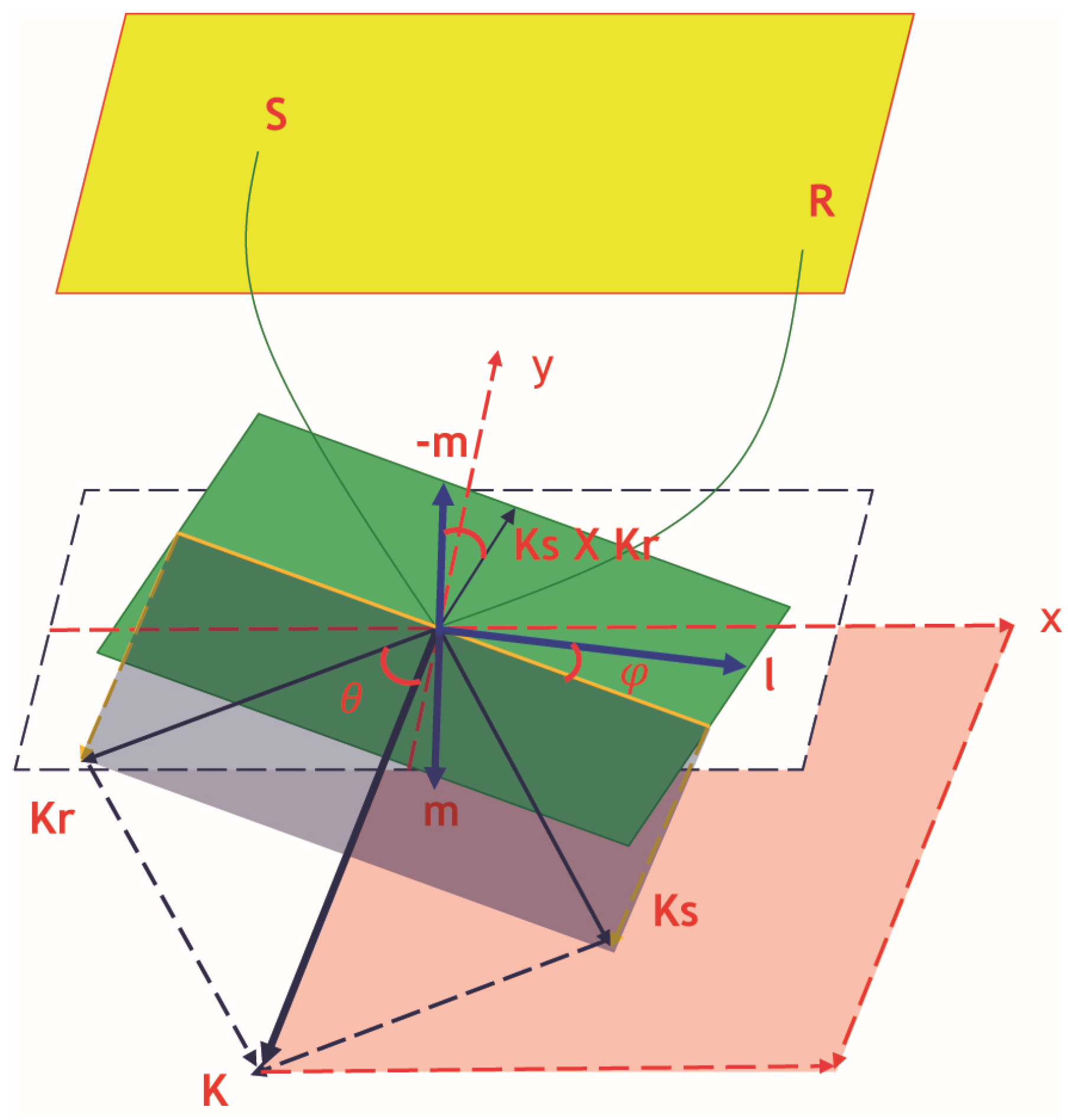
2.3. Method for Computing the Subsurface Incident Angle and Azimuth

In this section, we will introduce how to compute the subsurface angles. In Figure 2, the wavenumber vectors ${\mathit{k}}_{\mathit{s}}$ and ${\mathit{k}}_{\mathit{r}}$ give the propagation directions at the image point for the wavefields from the source and receiver locations, respectively. The vector $\mathit{k}$ is the migration vector computed by $\mathit{k}={\mathit{k}}_{\mathit{s}}+{\mathit{k}}_{\mathit{r}}$; in the specular cases, it coincides with the reflector’s normal vector. The $\theta$ is the reflection opening angle, and $\phi$ is the reflection azimuth angle. Our conventions of subsurface reflection opening and azimuth angle are similar to those of Xu et al. (2011) [13]. In that paper, the subsurface incident angle is computed by Equation (3). The azimuth angle is calculated by Equation (4), where the unit vector is defined as ${\mathit{n}}_{\mathit{x}}=(\mathrm{1,0},0)$. Note that although there are three vectors in Equation (4), only two vectors need to be computed, and the remaining one can be derived from the other two.

$$\cos \theta ={\displaystyle \frac{\mathit{k}·{\mathit{k}}_{\mathit{r}}}{\left|\mathit{k}\right|\left|{\mathit{k}}_{\mathit{r}}\right|}}$$

(3)

$$\cos \phi ={\displaystyle \frac{\left({\mathit{k}}_{\mathit{s}}\times {\mathit{k}}_{\mathit{r}}\right)·\left({\mathit{n}}_{\mathit{x}}\times \mathit{k}\right)}{\left|{\mathit{k}}_{\mathit{s}}\times {\mathit{k}}_{\mathit{r}}\right|\left|{\mathit{n}}_{\mathit{x}}\times \mathit{k}\right|}}$$

(4)

To compute the reflection opening angle, Equation (3) is correct, and we use the same equation in this paper. For the subsurface reflection azimuth angle, if the source and receiver locations change, the azimuth angle should be the same. In Equation (4), the vector ${\mathit{k}}_{\mathit{s}}\times {\mathit{k}}_{\mathit{r}}$ will have an opposite sign if we shift the shot and receiver positions. To solve this issue, we derive a new formula in Equations (5)–(8) to compute the azimuth angle.

$$\mathit{l}=\left(\mathit{k}\times {\mathit{n}}_{\mathit{x}}\right)\times \mathit{k},\mathit{m}=\mathit{k}\times \mathit{l}$$

(5)

$$p=-{\displaystyle \frac{\left({\mathit{k}}_{\mathit{s}}\times {\mathit{k}}_{\mathit{r}}\right)·\mathit{m}}{\left|{\mathit{k}}_{\mathit{s}}\times {\mathit{k}}_{\mathit{r}}\right|\left|\mathit{m}\right|}}$$

(6)

$$q={\displaystyle \frac{\left({\mathit{k}}_{\mathit{s}}\times {\mathit{k}}_{\mathit{r}}\right)·\mathit{l}}{\left|{\mathit{k}}_{\mathit{s}}\times {\mathit{k}}_{\mathit{r}}\right|\left|\mathit{l}\right|}}$$

(7)

$$\phi =mod\left(2\pi +sign\left(q\right){\mathrm{c}\mathrm{o}\mathrm{s}}^{-1}\left(p\right),N\pi \right)$$

(8)

The green plane in Figure 2 is the reflection plane which represents the final stacked image, and vectors ${\mathit{k}}_{\mathit{s}}\times {\mathit{k}}_{\mathit{r}}$, $\mathit{m}$, and $\mathit{l}$ are all at the reflection plane. For better understanding, vector $\mathit{l}$ is the projection of the plane formed by the migration vector $\mathit{k}$ and the unit vector ${\mathit{n}}_{\mathit{x}}$. Vector $\mathit{m}$ is also in the reflection plane, and it is perpendicular to $\mathit{l}$. In Equation (8), the parameter $N$ equals one if we limit the azimuth angle to the range $0~\pi$, and two if we limit the azimuth angle to the range $0~2\pi$.

In Figure 3, we design a synthetic example to validate Equations (5)–(8) for computing the azimuth angle. Only one shot is used with a maximum offset of 4 km in both horizontal directions, and three reflection events exist for computing the shot gather. In Figure 3a, the shot position is at the center of the acquisition geometry. The red, green, purple, and black circles indicate the image location for computing the ADCIGs for validation. Figure 3b is the shot gather with a red line showing receiver locations in Figure 3a.

In Figure 4, we compute the ADCIGs for the four locations indicated by the color circles in Figure 3a. All the incident angles are calculated using Equation (3), and the computed angles are consistent with the analytical solutions. If we calculate the azimuth using Equation (4), the ADCIGs for the red and green circle locations will be in Figure 4a, while the purple and black spots will be in Figure 4b. The results are incorrect because the reciprocity is not satisfied. If we use Equation (8) to recompute the azimuth, the ADCIGs for the red and purple circles will be as shown in Figure 4a, and the green and black circles will be as shown in Figure 4b, which is more reasonable. In this example, we limit the azimuth range to $0~\pi$.

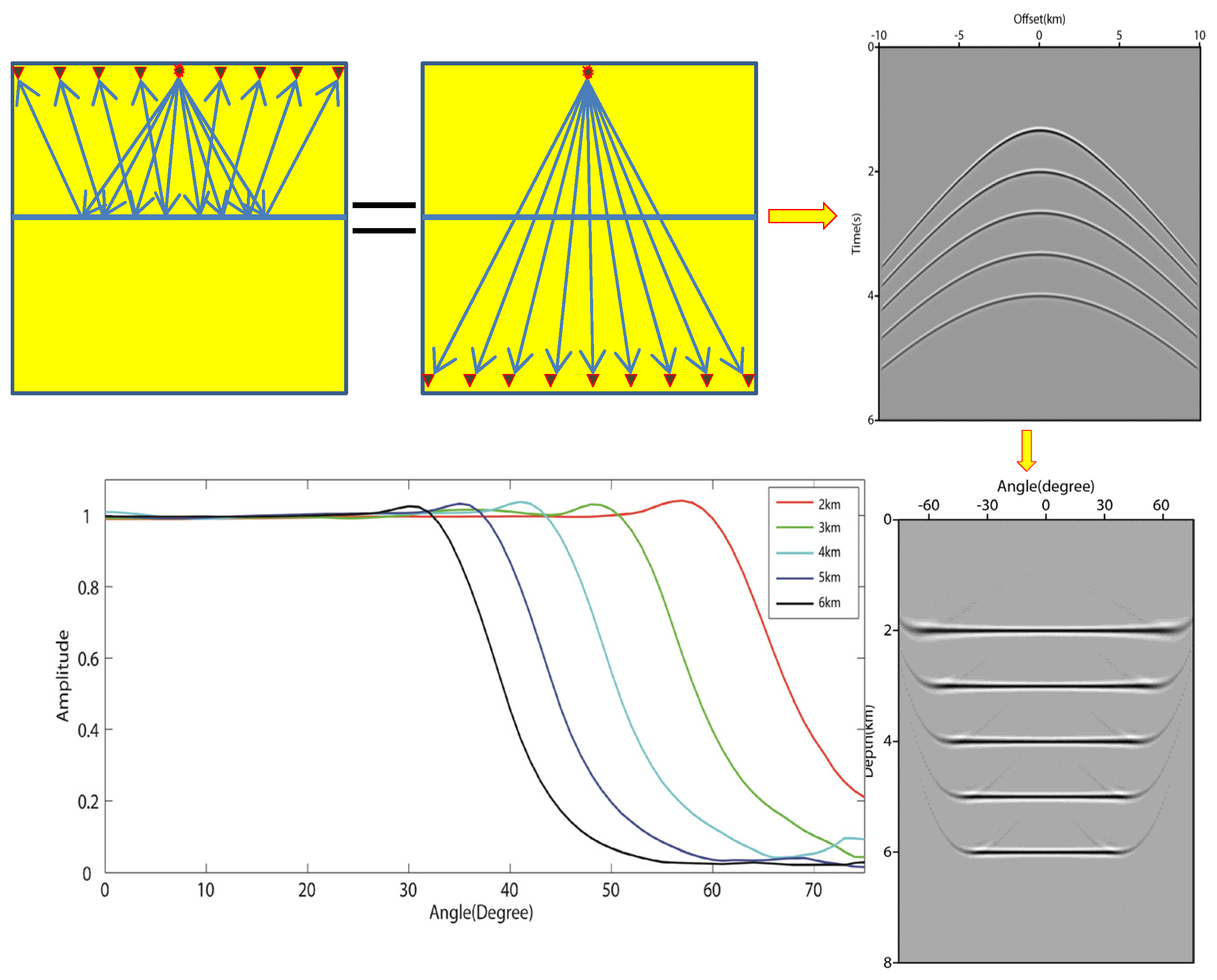
2.4. Angle Domain Illumination Compensation Factor for Constant Medium

This section addresses two issues related to the imaging condition in Equation (1) and the angle binning in Equation (2). Firstly, the singularity in the imaging condition can cause difficulties in accurate amplitude preservation. Secondly, the angle binning equation does not consider the acquisition geometry, leading to potential distortions in the angle domain image. To overcome these challenges, we introduce the angle domain illumination factor, which aims to mitigate the singularity and incorporate acquisition geometry information for improved amplitude preservation in the angle domain.

For a constant medium, we introduce an angle domain illumination compensation factor $W\left({\theta }_0,{\phi }_0\right)$ into Equation (2) for angle domain binning. We assume only one incident angle for each imaging location from each shot. In Equation (5), $N_{true}$ is the actual number of hits for each output bin of each imaging location, which is computed during the angle binning; $N_{ideal}$ is the ideal illumination hit count number, which is proportional to the area of the blue fan in Figure 5. Without giving the detailed mathematical derivation, $N_{ideal}$ can be calculated using Equation (6). In this equation, $∆\theta$ and $∆\phi$ are the binning size, and $Z$ is the depth of the imaging location. Substituting Equations (1) and (5)–(8) into Equation (2), and we can find that the issue of singularity at $\theta =0^o$ is solved.

$$\stackrel{̿}{R}\left(\mathbf{x},{\theta }_0,{\phi }_0\right)=\int {W\left({\theta }_0,{\phi }_0\right)\overline{R}}_s\left(\mathbf{x},{\theta }_0,{\phi }_0\right)ds$$

(9)

$$W\left({\theta }_0,{\phi }_0\right)={\displaystyle \frac{N_{ideal}}{N_{true}}}$$

(10)

$$N_{ideal}=Z^2{\displaystyle \frac{\mathrm{s}\mathrm{i}\mathrm{n}\theta }{{\left(\mathrm{c}\mathrm{o}\mathrm{s}\theta \right)}^3}}∆\theta ∆\phi$$

(11)

2.5. Angle Domain Illumination Compensation Factor for v(z) Medium

For a more general case, we introduce the angle domain illumination compensation factor for a vertically increasing velocity medium with $v^{\prime }$ as the velocity gradient along the vertical direction. The factor is the same as Equation (5), but the ideal illumination number $N_{ideal}$ is calculated using Equation (12). In this equation, $r_2$ and $r_1$ are the inner and outer radii of the blue fan shape. In the following equations, $p_1$ and $p_1^{\prime }$ are the ray parameters of the rays according the inner and outer radii, ${\theta }_1$ and ${\theta }_1^{\prime }$ are the incident angles at the acquisition surface, ${\theta }_2$ and ${\theta }_2+∆\theta$ are the incident angles at the subsurface image location, $v_0$ is the velocity of the acquisition surface, and $∆\theta$ and $∆\phi$ are the binning size.

$$N_{ideal}=\left(r_1^2-r_2^2\right)∆\phi /2$$

(12)

$$r_1=\left({\displaystyle \frac{1}{p_1{v}^{\prime }}}\left(\cos {\theta }_1-\cos {\theta }_2\right)\right)$$

(13)

$${\theta }_1={\sin }^{-1}\left(v_0{p}_1\right)$$

(14)

$$r_2=\left({\displaystyle \frac{1}{{p_1^{\prime }v}^{\prime }}}\left(\cos {\theta }_1^{\prime }-\cos \left({\theta }_2+∆\theta \right)\right)\right)$$

(15)

$${\theta }_1^{\prime }={\sin }^{-1}\left(v_0{p}_1^{\prime }\right)$$

(16)

3. Results

In this section, we validate the angle domain illumination compensation factor concept for irregular acquisition geometries by applying Equations (12)–(16) to synthetic and field data examples. By incorporating this factor, we aim to mitigate the amplitude errors caused by irregular acquisition geometries and ensure the preservation of amplitude information in the prestack ADCIGs. By analyzing synthetic and real-world field data, we assess the effectiveness of the angle domain illumination compensation factor and its ability to address the challenges posed by non-uniform acquisition geometries.

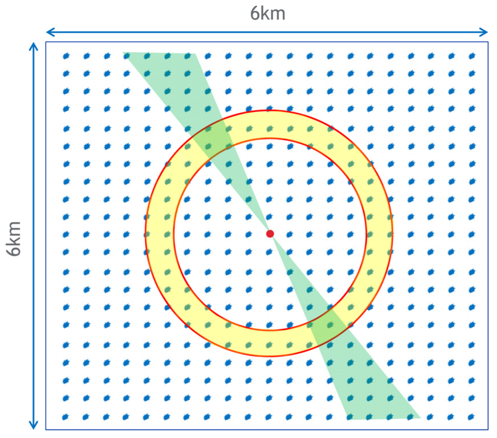
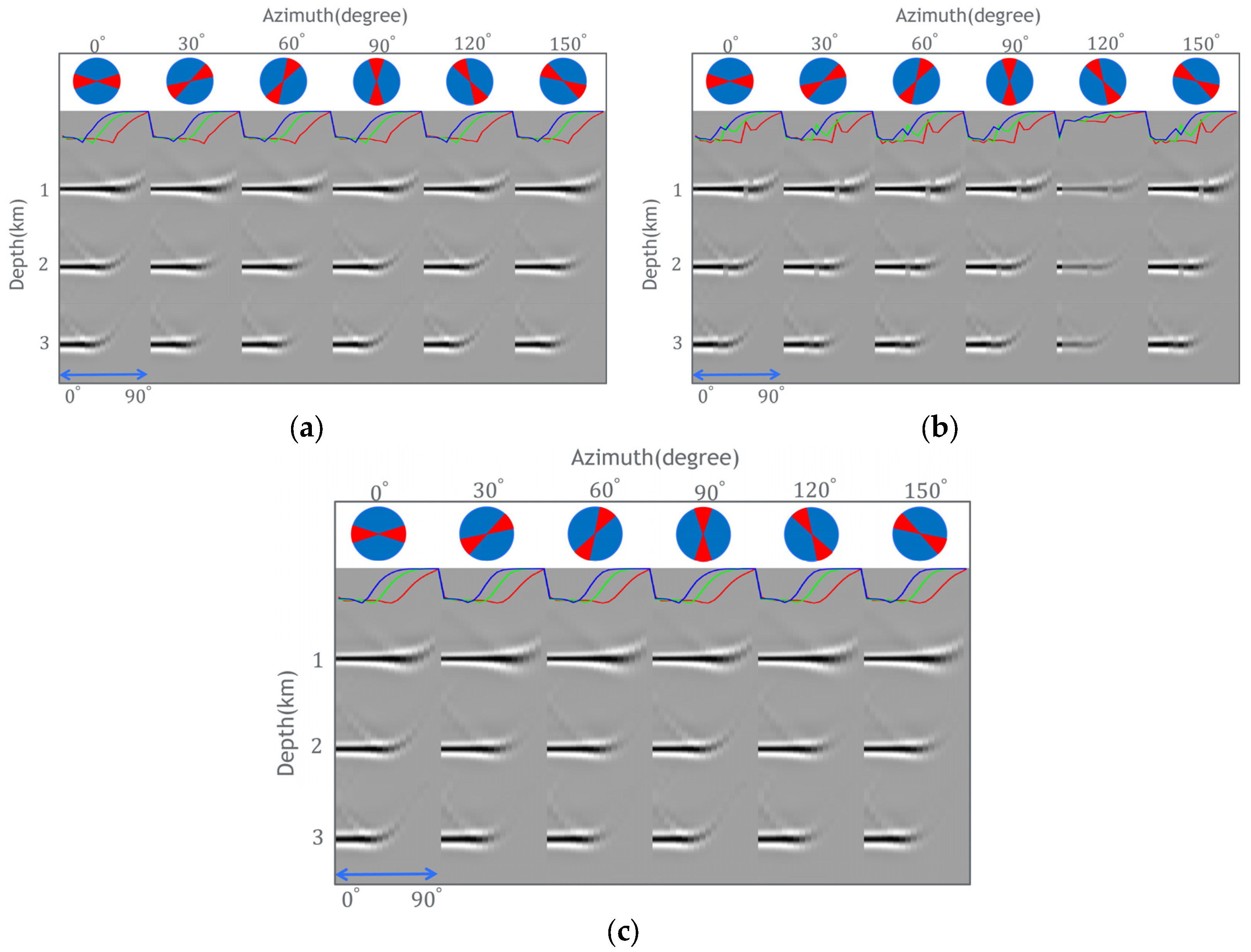
3.1. Synthetic Example

We use the virtual interface method [14] to generate the synthetic data. Since there is no actual interface, the reflection coefficients from the virtual interface are constant for any incidence angle. This virtual reflection is beneficial for testing the true-amplitude RTM algorithm—the amplitudes in a migrated ADCIG are independent of the incidence angles.

We simulate three virtual interfaces to perform ADCIG tests. The velocity of the medium is $2000+0.3Z$. Figure 6 shows the acquisition geometry, where shots are missing while receivers are regularly distributed. These missing shots introduce irregularities and challenges in the acquisition geometry, which we aim to address and account for in our analysis and evaluation. Figure 7a shows the ADCIGs of the target point, shown as a red dot in Figure 6 using the regular geometry data as input. The color curves in this Figure show that the maximum amplitude for the reflectors at 1 km, 2 km, and 3 km are preserved. By removing part of the shots as shown in Figure 6, the amplitudes are not preserved anymore, as shown in Figure 7b. After applying the angle domain illumination compensation factor, the flatness of the amplitude curves is well recovered as shown in Figure 7c.

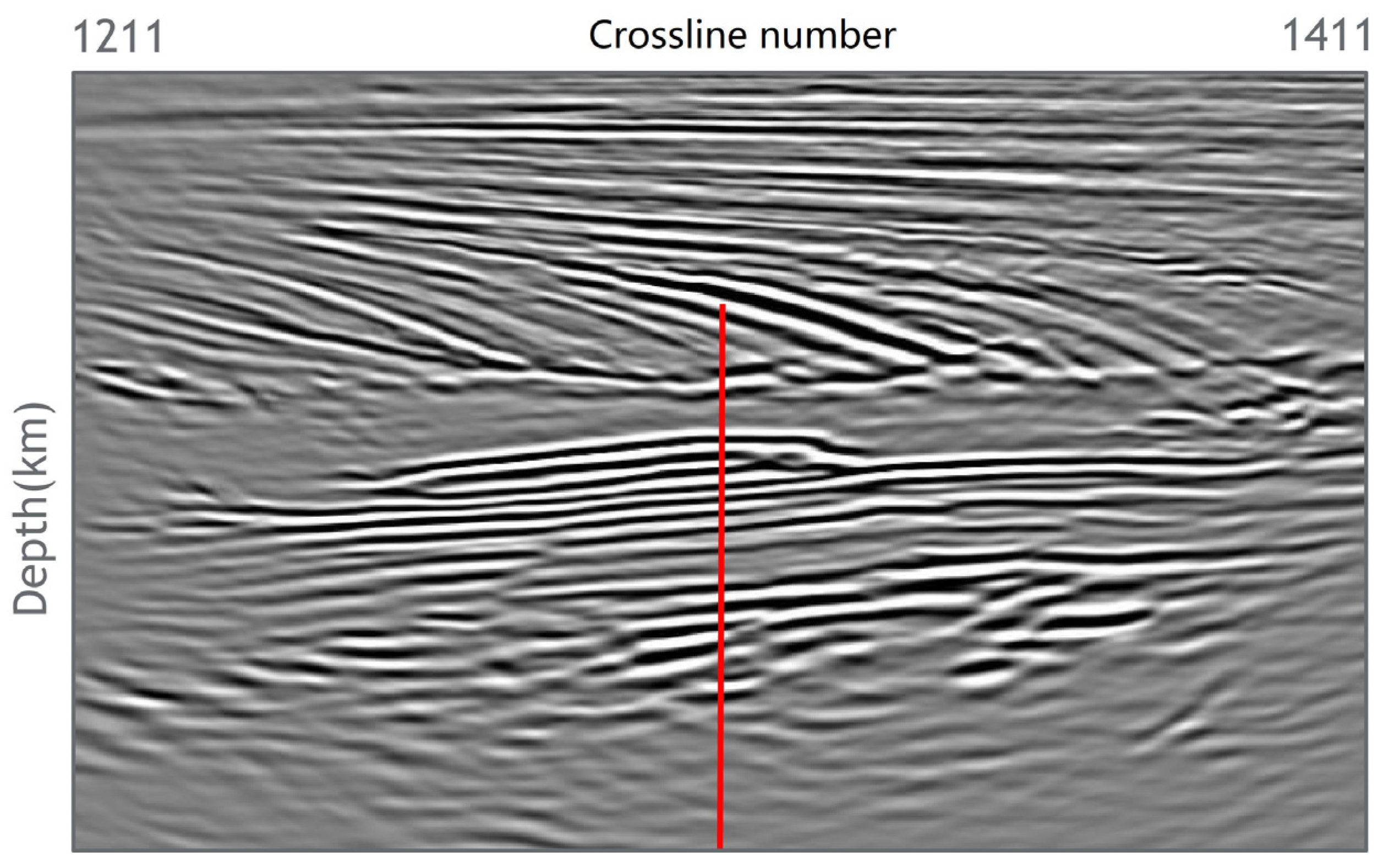
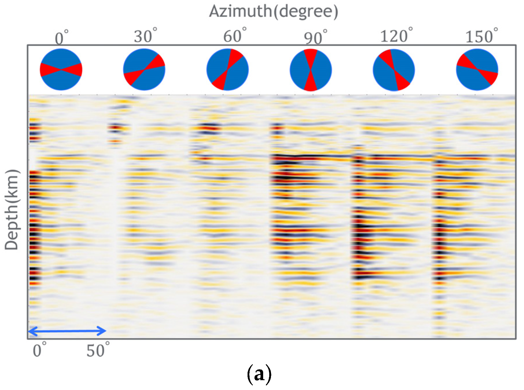
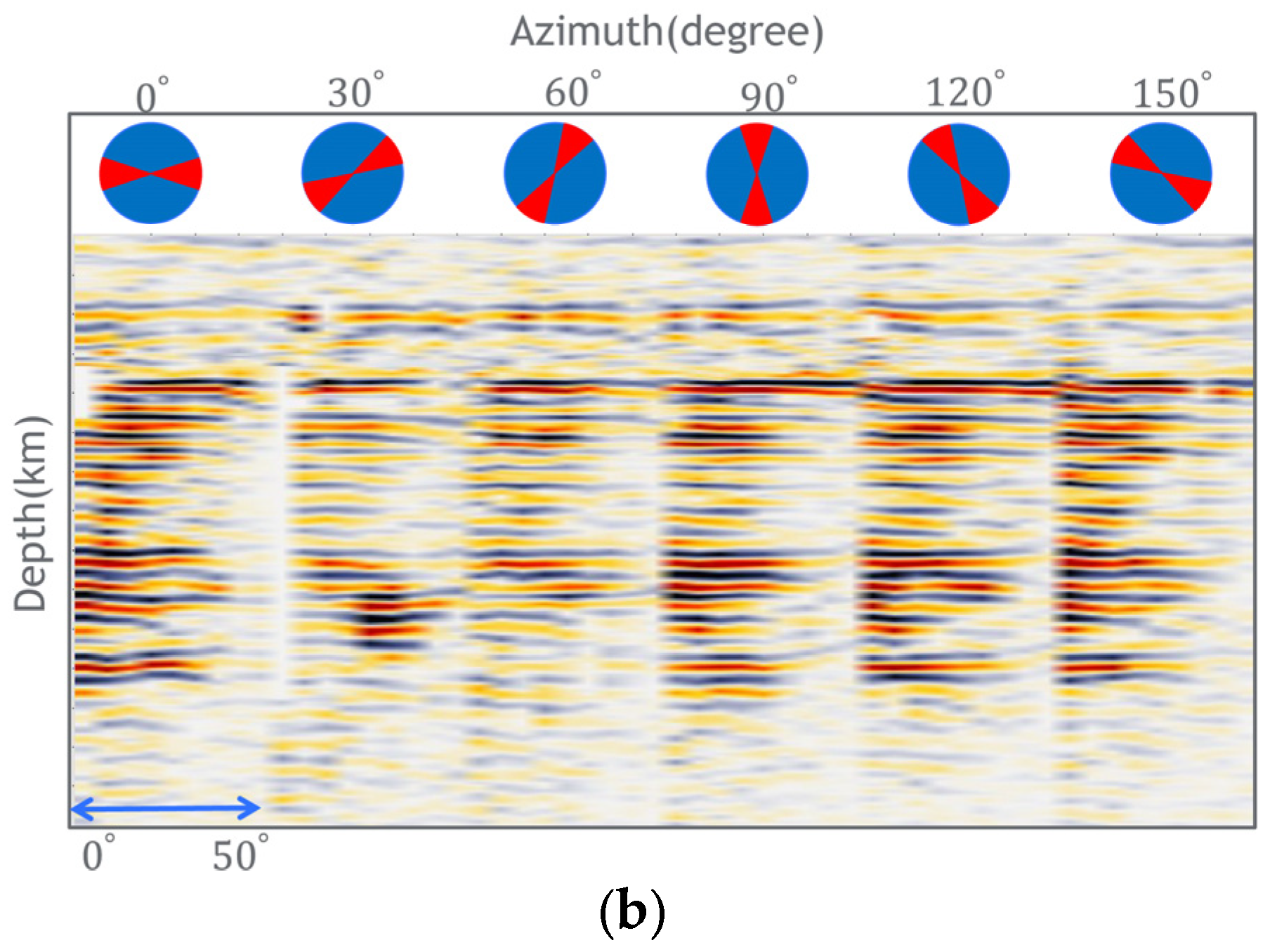
3.2. Field Data Example

In the transition zone of the Middle East, where this project is located, seismic vibrators are used as sources onshore, while no shooting is conducted offshore. The target location of interest is situated in the full fold limit area, where performing AVA analysis is crucial. Figure 8 showcases the inline RTM stacked image obtained across the target location. This image results from the RTM process, which involves migrating the seismic data to generate a focused and coherent representation of the subsurface. The RTM stacked image in Figure 8 provides valuable insights into the subsurface structures and features within the target area. It serves as a foundation for further analysis, including AVA analysis, which will help assess the variations in seismic amplitudes with different incident angles. Such analysis can provide valuable information about the area’s reservoir properties and potential hydrocarbon-bearing formations.

Figure 9a represents the ADCIGs obtained for the target location using the imaging condition described by Equation (1) before applying the angle domain illumination compensation factor. This figure shows that the energy for azimuth angles of 0°, 30°, and 60° is significantly weaker than that for other azimuth angles. This is primarily due to the missing shots corresponding to these azimuth locations, resulting in incomplete coverage and reduced energy in those directions. Another issue observed in Figure 9a is the imbalance in energy for different incidence angles. The energy for slight incidence angles appears much stronger than that for larger ones. This uneven distribution of energy is caused by the singularity at $\theta =0^o$, which affects the amplitude calculation and leads to a distorted representation of the subsurface features.

To address these issues and achieve a more balanced and accurate representation of the ADCIGs, the angle domain illumination compensation factor is employed. After incorporating this compensation factor, Figure 9b demonstrates a significant improvement in the amplitude distribution across different incident and azimuth angles. The compensation factor helps to mitigate the impact of missing shots and the singularity, resulting in a more balanced representation of energy across various angles. The ADCIG in Figure 9b provides a more reliable basis for subsequent AVA analysis and other interpretation tasks by applying the angle domain illumination compensation factor. It ensures that the amplitude information is preserved and allows a more accurate assessment of subsurface properties and reservoir characteristics in the target location.

4. Discussion

The angle domain illumination compensation factor introduced in this paper offers a solution to address amplitude errors resulting from irregular seismic acquisition geometries. By applying this compensation factor in the 3D RTM process, the resulting ADCIG can effectively preserve the amplitude of the seismic reflectivity. This preserved amplitude information is valuable for prestack AVA analysis, which plays a crucial role in reservoir characterization. The compensation factor resolves the irregular geometry issue and addresses the singularity problem associated with traditional true-amplitude RTM imaging conditions. By incorporating the compensation factor, the singularity problem is mitigated, leading to a more accurate representation of amplitudes in the migrated images. It is also worth mentioning that the introduced compensation factor does not change the conventional workflow of other methods for improving seismic imaging of the ADCIGs in the processes of signal amplification, its filtering, and post-stack processing.

5. Conclusions

The compensation factor in this paper is based on a 1D velocity model assumption, and an analytical solution is utilized, resulting in negligible additional computational cost compared to methods without compensation. While the proposed method primarily focuses on resolving issues related to irregular surface acquisition geometries, the principle behind the compensation factor can be extended to more complex subsurface media and various migration methods by employing numerical approaches to calculate the compensation factor.

In summary, the introduced angle domain illumination compensation factor provides a practical and effective means to address amplitude errors caused by irregular seismic acquisition geometries. The method can be extended to handle complex subsurface media using numerical techniques, offering flexibility and applicability in a broader range of scenarios.

References

1. Liu, H.; Li, B.; Tong, X.; Liu, Q. The algorithm of high order finite difference pre-stack reverse time migration and GPU implementation. Chin. J. Geophys. 2010, 53, 1725–1733. [Google Scholar] [CrossRef]
2. Liu, H.; Li, B.; Liu, H.; Tong, X.; Liu, Q.; Wang, X.; Liu, W. The issues of pre-stack reverse time migration and solutions with GPU implementation. Geophys. Prospect. 2012, 60, 906–918. [Google Scholar] [CrossRef]
3. Liu, H.; Liu, H.; Tong, X.; Liu, Q. A Fourier integral algorithm and its GPU/CPU collaborative implementation for one-way wave equation migration. Comput. Geosci. 2012, 45, 139–148. [Google Scholar] [CrossRef]
4. Liu, H.; Zhang, H. reducing computation cost by Lax-Wendroff methods with fourth-order temporal accuracy. Geophysics 2019, 84, T109–T119. [Google Scholar] [CrossRef]
5. Zhang, Y.; Sun, J. Practical issues of reverse time migration: True-amplitude gathers, noise removal and harmonic-source encoding. First Break 2009, 26, 19–25. [Google Scholar] [CrossRef]
6. Shan, G.; Biondi, B. Angle-domain common-image gathers for steep reflectors. In Proceedings of the 78th Annual International Meeting, SEG, Expanded Abstracts, Las Vegas, NV, USA, 9–14 November 2008; pp. 3068–3072. [Google Scholar] [CrossRef]
7. Bleistein, N.; Cohen, J.K.; Stockwell, J.W. Mathematics of Multidimensional Seismic Inversion; Springer: Berlin/Heidelberg, Germany, 2001. [Google Scholar]
8. Xu, S.; Chauris, H.; Lambaré, G.; Noble, M. Common angle migration: A strategy for imaging complex media. Geophysics 2001, 66, 1877–1894. [Google Scholar] [CrossRef]
9. Zhang, Y.; Zhang, G.; Bleistein, N. Theory of true-amplitude one-way wave equations and true-amplitude common-shot migration. Geophysics 2005, 70, E1–E10. [Google Scholar] [CrossRef]
10. Zhang, Y.; Xu, S.; Bleistein, N.; Zhang, G. True-amplitude, angle-domain, common-image gathers from one-way wave-equation migrations. Geophysics 2007, 72, S49–S58. [Google Scholar] [CrossRef]
11. Biondi, B.; Symes, W.W. Angle-domain common-image gathers for migration velocity analysis by wavefield-continuation imaging. Geophysics 2004, 69, 1283–1298. [Google Scholar] [CrossRef]
12. Jin, H.; McMechan, G.A.; Guan, H. Comparison of methods for extracting ADCIGs from RTM. Geophysics 2014, 79, S89–S103. [Google Scholar] [CrossRef]
13. Xu, S.; Zhang, Y.; Tang, B. 3D angle gathers from reverse time migration. Geophysics 2011, 76, S77–S92. [Google Scholar] [CrossRef]
14. Liu, H.; Luo, Y. Invertible radon transform for making true amplitude angle gathers. In Proceedings of the SEG Technical Program Expanded Abstracts, New Orleans, LA, USA, 18–23 October 2015; pp. 4158–4163. [Google Scholar] [CrossRef]
15. Zhang, Y.; Xu, S.; Tang, B.; Bai, B.; Huang, Y.; Huang, T. Angle gathers from reverse time migration. Lead. Edge 2010, 29, 1364–1371. [Google Scholar] [CrossRef]
16. Luo, M.; Lu, R.; Winbow, G.; Bear, L. A comparison of methods for obtaining local image gathers in depth migration. In Proceedings of the 80th Annual International Meeting, SEG, Expanded Abstracts, Denver, CO, USA, 17–22 October 2010; pp. 3247–3251. [Google Scholar] [CrossRef]
17. Sava, P.; Fomel, S. Angle-gathers by Fourier transform. Stanf. Explor. Proj. Rep. 2000, 103, 119–130. [Google Scholar]
18. Sava, P.; Fomel, S. Angle-domain common-image gathers by wavefield continuation methods. Geophysics 2003, 68, 1065–1074. [Google Scholar] [CrossRef]
19. Sava, P.; Fomel, S. Time-shift imaging condition in seismic migration. Geophysics 2006, 71, S209–S217. [Google Scholar] [CrossRef]
20. Xie, X.; Wu, R.S. Extracting angle domain information from migrated wavefields. In Proceedings of the 72nd Annual International Meeting, SEG, Expanded Abstracts, Salt Lake City, UT, USA, 29 September–2 October 2002; pp. 1360–1363. [Google Scholar] [CrossRef]
21. Yan, R.; Xie, X. A new angle-domain imaging condition for reverse time migration. In Proceedings of the 79th Annual International Meeting, SEG, Expanded Abstracts, Houston, TX, USA, 25–30 October 2009; pp. 2784–2788. [Google Scholar] [CrossRef]
22. Yan, R.; Xie, X. An angle-domain imaging condition for elastic reverse time migration and its application to angle gather extraction. Geophysics 2012, 77, S105–S115. [Google Scholar] [CrossRef]
23. Yoon, K.; Guo, M.; Cai, J.; Wang, B. 3D RTM angle gathers from source wave propagation direction and dip of reflector. In Proceedings of the 81st Annual International Meeting, SEG, Expanded Abstracts, San Antonio, TX, USA, 18–23 September 2011; pp. 1057–1060. [Google Scholar] [CrossRef]
24. Tang, C.; McMechan, G.A. Multi directional-vector-based elastic reverse time migration and angle-domain common-image gathers with approximate wavefield decomposition of P-and S-waves. Geophysics 2017, 83, S57–S79. [Google Scholar] [CrossRef]
25. Schuster, G.T. Least-squares cross-well migration. In Proceedings of the 63rd Annual International Meeting, SEG, Expanded Abstracts, Washington, DC, USA, 26–30 September 1993; pp. 110–113. [Google Scholar] [CrossRef]
26. Luo, Y.; Wang, Y.; AlBinHassan, N.; Alfaraj, M. Computation of dips and azimuths with weighted structural tensor approach. Geophysics 2006, 71, V119–S121. [Google Scholar] [CrossRef]
Figure 1. The concept of the amplitude-preserving ADCIG method. The top left figure demonstrates the generation of synthetic data with constant reflection coefficients, representing an ideal scenario for testing amplitude preservation. The top right figure displays a single shot gather with five virtual interfaces, each characterized by different reflection coefficients. The bottom right figure depicts the ADCIG for a specific image location, which provides prestack underground illumination information. Finally, the bottom left figure shows the relative peak amplitude obtained from the five virtual events, highlighting the amplitude variations within the ADCIG.
Remotesensing 16 03362 g001
Figure 2. Definition of angles. The wavenumber vectors k s and k r give the propagation directions at the image point for the wavefields from the source and receiver locations, respectively. The vector k is the migration vector; in the specular cases, it coincides with the reflector normal vector. θ is the reflection opening angle and φ is the reflection azimuth angle. The green plane is the reflection plane which represents the final stacked image, Vectors k s × k r , m , and l are all in the reflection plane.
Remotesensing 16 03362 g002
Figure 3. Shot gather used for validating the azimuth angle computation. (a) is the geometry with the shot position at the center, surrounded by receivers with a maximum offset of 4 km in both directions. The red, green, purple, and black circles indicate the image location for computing ADCIGs. (b) shows the shot gather, indicated by the red lines in (a).
Remotesensing 16 03362 g003
Figure 4. ADCIG result for azimuth computation validation. (a) is the ADCIG for the red and purple locations, and (b) is the ADCIG for the green and black points using the new method. These ADCIGs were generated using the newly derived method for azimuth computation.
Remotesensing 16 03362 g004
Figure 5. Angle domain illumination compensation factor for constant medium in (a) and vertical linear increasing velocity medium in (b).
Remotesensing 16 03362 g005
Figure 6. Acquisition geometry for the synthetic test. The central red point represents the target location of interest. The blue dots indicate the positions of the shots used in the acquisition. However, the yellow circle area represents a specific region within an offset range of 2 km to 2.3 km, where shots are missing. Additionally, shots are not present within an azimuth range of 105° to 125°, denoted by the green triangle area.
Remotesensing 16 03362 g006
Figure 7. The RTM ADCIGs using the data with regular (a) and irregular acquisition geometry (b) before and (c) after the illumination compensation factor. The red, green, and blue curves display the maximum amplitude for the reflectors at 1 km, 2 km, and 3 km, respectively.
Remotesensing 16 03362 g007
Figure 8. The stacked RTM image at the target location. The red line is the location for the ADCIG shown in Figure 9.
Remotesensing 16 03362 g008
Figure 9. The RTM ADCIGs before (a) and after (b) the illumination compensation factor.
Remotesensing 16 03362 g009aRemotesensing 16 03362 g009b
Disclaimer/Publisher’s Note: The statements, opinions and data contained in all publications are solely those of the individual author(s) and contributor(s) and not of MDPI and/or the editor(s). MDPI and/or the editor(s) disclaim responsibility for any injury to people or property resulting from any ideas, methods, instructions or products referred to in the content.