Mapping Fruit-Tree Plantation Using Sentinel-1/2 Time Series Images with Multi-Index Entropy Weighting Dynamic Time Warping Method

Abstract

Plantation distribution information is of great significance to the government’s macro-control, optimization of planting layout, and realization of efficient agricultural production. Existing studies primarily relied on high spatiotemporal resolution remote sensing data to address same-spectrum, different-object classification by extracting phenological information from temporal imagery. However, the classification problem of orchard or artificial forest, where the spectral and textural features are similar and their phenological characteristics are alike, still presents a substantial challenge. To address this challenge, we innovatively proposed a multi-index entropy weighting DTW method (ETW-DTW), building upon the traditional DTW method with single-feature inputs. In contrast to previous DTW classification approaches, this method introduces multi-band information and utilizes entropy weighting to increase the inter-class distances. This allowed for accurate classification of orchard categories, even in scenarios where the spectral textures were similar and the phenology was alike. We also investigated the impact of fusing optical and Synthetic Aperture Radar (SAR) data on the classification accuracy. By combining Sentinel-1 and Sentinel-2 time series imagery, we validated the enhanced classification effectiveness with the inclusion of SAR data. The experimental results demonstrated a noticeable improvement in orchard classification accuracy under conditions of similar spectral characteristics and phenological patterns, providing comprehensive information for orchard mapping. Additionally, we further explored the improvement in results based on two different parcel-based classification strategies compared to pixel-based classification methods. By comparing the classification results, we found that the parcel-based averaging method has advantages in clearly defining orchard boundaries and reducing noise interference. In conclusion, the introduction of the ETW-DTW method is of significant practical importance in addressing the challenge of same-spectrum, different-object classification. The obtained orchard distribution can provide valuable information for the government to optimize the planting structure and layout and regulate the macroeconomic benefits of the fruit industry.

1. Introduction

The fruit industry plays a significate role in improving land productivity and economic conditions of farmers [1]. In 2019, China’s fruit tree planting area was about 1227 hectares, with an output of about 190 million tons (National Bureau of Statistics data, https://www.stats.gov.cn/ [accessed on 12 March 2024]), ranking first in the world for many years. In areas such as Shaanxi Province and Shanxi Province, the fruit industry has become a pillar industry of the local economy. In realizing the sustainable development of fruit production, quantifying the spatial scope and growth time dynamics of orchards will help the government to better optimize resource distribution and the planting structure. Based on the traditional ground sampling survey method, a lot of personnel and material resources are required, and real-time orchard distribution and health status information cannot be obtained [2]. Satellite remote sensing technology has long been used to assess the dynamics of land ecosystems [3,4,5] and is suitable for capturing the changing events of geophysical processes due to its rich data volume on spatial and temporal scales [6,7,8,9,10]. With the continuous development of satellite sensor technology, the spatial and temporal resolutions of remote sensing images are continuously optimized, and satellite remote sensing has become an efficient and accurate means of monitoring large-scale farmland [11,12,13].

Satellite image classification based on single-temporal data may not be satisfactory in complex crop-growing systems [14]. Time-series satellite image data can capture the seasonal characteristics of horticulture crops. Through long-term observation of satellite images, different phenological features that can characterize crop development can be extracted, which is one of the methods to solve the bottleneck of crop classification accuracy [15]. Moderate resolution images such as Landsat, IKONOS, and SPOTS were widely used to distinguish crop planting intensity and planting structure extraction at a field scale [16,17]. EI et al. [18] used SPOTS-5 time series images as a data source to extract the distribution and harvest of sugarcane. Murakanmi et al. [19] implemented crop identification with multitemporal HRV data. However, during the growth stage of crops, soil surface and vegetation growth conditions vary with the seasons and field conditions. Capturing these differences is an essential element in identifying land use types, and obtaining more high-quality images is crucial [20].

Despite recent progress, the temporal resolution of optical images limited crop development throughout the growing season due to cloud cover [17]. Fortunately, synthetic aperture radar (SAR) satellites, such as Sentinel-1, are not affected by cloudy and rainy weather and can provide reliable long-term observations for monitoring crop growth [21,22]. Some studies have tried to classify crop types using Sentinel-1 dual polarimetry imagery [23]. SAR satellites are capable of the penetration of waves into the ground (few centimeters), capturing backscattering images of different types of vegetation, monitoring ground roughness and capturing the geometry associated with vegetation canopy structure [24]. The complementarity of optical and radar data enhances the overall performance of land cover classification. In different scenarios, these combinations can achieve higher accuracy results, such as crop monitoring [25], grassland monitoring [26], wildfire assessment [27], and invasive plant monitoring [28].

In regard to crop type mapping, existing methods can be mainly divided into two categories. The first type of method considers satellite image time series (SITS) as simple stacks of multiple features [29]. Such stacks of features have been applied to machine learning (ML) algorithms for classification, including decision tree (DT) [30], random forest (RF) [31], and support vector machine (SVM) [32]. However, these methods have no strategy to extract phenological information into a classification scheme, i.e., disrupting the stacking order of time series images will not improve the image classification performance. At the same time, machine learning methods have strong sample dependence and under the condition of a lack of samples, the classification performance may not be satisfactory.

The second type of time series classification method uses knowledge of phenology or time-varying features to describe temporal contextual information to improve crop identification [33]. For expressing the temporal dependencies of the time-series datasets caused by crop phenology [34,35], the phenological sequence pattern (PSP) method [36], Conditional Random Fields (CRF) [37] and Hidden Markov Model (HMM) [38] have been applied to crop mapping as statistical models. However, the above methods combined with phenology knowledge are still difficult to apply for crop mapping. In practical applications, there are three main obstacles: (1) drawbacks in sample availability that can be overcome by reference to past data; (2) irregular temporal sampling of images and missing information in the dataset (e.g., cloud pollution) can obscure the analysis [39]; and (3) variability in proposed periodic phenomena (e.g., vegetation cycles influenced by weather conditions). Such uncertainty is usually caused by random variation in agroclimatic conditions and agricultural practices, which manifests itself as a misalignment of time series from a particular crop type to different plots [33,40,41].

Dynamic Time Warping (DTW) has been proven to be a suitable classifier to solve the above problem, as it allows for taking the similarity of temporal sequences into account as a function of crop phenology [42]. Each land-cover class has a distinct phenological cycle that is relevant for space-time classification. The DTW method warps time to match the two series and the DTW distance is calculated as resemblance measure for the two temporal profiles [39]. Recently, DTW has become a focus for remote sensing classification [43]. Petitjean et al. [41] presented a method based on Formosat-2 for image time series analysis that is able to handle irregularly sampled sequences using DTW theories. Dong et al. [44] proposed a phenology time-weighted DTW (PT-DTW) method that needed less sampling effort for Sentinel 2A/B time series images, and a specific vegetation index was suggested for mapping winter wheat. Maus et al. [42] introduced a time-weighted DTW method (TWDTW) to classify crops with an Enhanced Vegetation Index (EVI) from MODIS data. Gella et al. [45] investigated DTW strategies to classify crops in complex farming areas using Sentinel-1 dual polarimetry (VV + VH) and TerraSAR-X single polarimetry (HH) images.

Building on the progress in crop mapping using the DTW algorithm, we added three issues that need further research: (1) Previous studies have examined optical and SAR images separately, but there is a lack of research on combining Sentinel-1 (S1) and Sentinel-2 (S2) imagery with long time-series using DTW theories; (2) For DTW classifiers, there has been limited exploration on complex agricultural land characterized by diverse crop types, close phenological stages, and intricate spatial patterns [39,45], especially for horticultural crops; and (3) The DTW classifiers typically utilize a single attribute feature as input, such as a single band or a single index. The lack of research on using multidimensional attributes as input severely limits its classification performance in complex scenarios.

For orchard classification, current research methods remain limited, despite the progress made by the aforementioned techniques in crop classification. The spectral confusion between orchards and native vegetation is a well-known challenge in forestry and tree crop systems [46]. Most studies have primarily focused on the extraction of single orchard types [43,47], using either single-date or time-series spectral features (such as optimal band selection [48], red-edge spectral indices (RESI) [47], and normalized difference indices (NDIs) [49]) to identify the most effective spectral combinations for distinguishing orchards from other land cover types. Texture information can effectively capture the spatial distribution characteristics of remote sensing images and mitigate the effects of the “same spectrum, different objects” or “same object, different spectra” phenomena. It has been proven to be effective in orchard classification [50,51]. Radar data responds differently to orchard canopy roughness, structure, and moisture content. When combined with optical imagery, it can significantly improve classification accuracy [52,53,54]. However, the fine-grained identification of multiple orchard types remains a challenge [52], as orchards such as apple and peach have similar planting structures and spectral characteristics, particularly during their phenological periods. Additionally, the fragmentation of orchard planting plots can introduce uncertainty in classification, further increasing the difficulty in distinguishing multiple orchard types.

To address the aforementioned issues, we proposed a classification method based on the TWDTW theory and leveraging entropy weighting to fuse multiple attributes (ETW-DTW). This method was applied to long time-series S1/2 imagery to extract orchard distributions with four closely related phenological stages and fragmented plots. Subsequently, we examined the contribution of SAR imagery to orchard classification, along with the impacts of pixel scale, post-processing scale, and parcel scale on the classification results. Finally, we discussed the strengths and limitations of the ETW-DTW algorithm in orchard classification and provided insights into future prospects.

2. Materials and Methods

2.1. Study Area and Datasets

The study area is located in Miaoshang Township, Qiji Township and Linjin Township (110°17′30.7″E–110°54′38.9″E 34°58′52.9″N–35°18′47.6″N) in the southern part of Linyi County, Shanxi Province. The area is in the Yuncheng Basin, with typical temperate continental climate characteristics, with four distinct seasons, more drought and less rain in spring and summer, more cloudy and rainy weather in autumn and more drought in winter. The county has sufficient sunshine and an average maximum daily temperature of 19.7 °C. Due to its excellent geographical and climatic conditions, it is very suitable for the growth of fruit crops and is known as the “Hometown of fruits” (Figure 1). Five major crops in the region were selected as classification targets: apples, jujubes, peaches, persimmon, and corn. The study area is characterized by narrow, fragmented planting plots with a relatively complex planting structure.

The phenological characteristics of crop types are the key elements for how to classify SITS data. Due to its unique geographical conditions, apples bloom ten days earlier than those in other major apple-growing areas in China, with flowering from late February to mid-April and fruiting in June, the fruit bulges from July to August and ripens from September to October. Peach trees bloom from March to early April, fruiting from April to May, and mature from June to September. The flowering period of jujube trees is May to July, the fruiting period is August, and the maturity period is September to October. The flowering period of persimmon trees is May to June, July to September, and the maturity period is October. Wheat and corn are planted in rotation (Figure 2).

2.2. Sentinel-1/2 Time Series Images Pre-Processing

As a kind of high-resolution remote sensing data, Sentinel satellite data provides a new opportunity for qualitative and quantitative monitoring of large-scale farmland [55]. Sentinel-2 (S2) satellites are composed of Sentinel-2A and Sentinel-2B, and the two satellites work together to make their revisit cycle reach five days. They carry a multi-spectral instrument (MSI), which can cover visible light, near-infrared to short-wave infrared. The number of bands is 13, including three red-edged bands that are beneficial for observing vegetation [56]. In this study, Google Earth Engine (GEE) was used to obtain the product of the Sentinel-2 Multi-Spectral Instrument, the Level 2A surface reflectance (“COPERNICUS/S2_SR”). A total of 69 Sentinel-2 L2A optical imaging products from November 2019 to December 2020 were selected in the study area (Figure 3a,b). In order to prevent the influence of rain and snow weather on the observation data throughout the year, a combination of six bands (Blue, Green, Red, NIR, SWIR1, and SWIR2), the Normalized Difference Snow Index (NDSI), and the Normalized Difference Moisture Index (NDMI) were used to calculate the cloud score and mask cloud and snow pixels in Sentinel-2 images. Finally, pixels contaminated by cloud shadows were removed based on solar geometry and cloud position, resulting in a high-quality observation image of the study area (Figure 3c).

The Sentinel-1 (S1) is an active microwave remote sensing data equipped with a synthetic aperture radar (SAR), which has the ability to penetrate clouds and is not susceptible to cloudy or rainy weather [57]. In this study, we used the Sentinel-1 Level 1 Ground Range Detected (GRD) product that uses the Wide swath (IW) mode providing data in VV (vertical transmit/vertical receive band of dual-polarization) and VH (vertical transmit/horizontal receive band of dual-polarization) polarizations. A total of 31 Sentinel-1 GRD products from November 2019 to December 2020 were selected in the study area (Figure 3b). The Sentinel-1 Toolbox (https://sentinel.esa.int/web/sentinel/toolboxes/sentinel-1/ [accessed on 1 April 2018]) was used to preprocess Sentinel-1 images to generate calibrated, ortho-corrected estimates of decibels via log scaling. The multi-looking is executed by averaging the cells and/or using resolution azimuths, thus increasing the radiometric resolution but decreasing the spatial resolution. “Scatter” (scattered noise level) is produced by interference that has a “salt and pepper” effect on the image. The speckle-filter is used to enhance the Lee filter proposed by Lee [58] with a window size of 7 × 7. Finally, the pixel-by-pixel backscattering coefficient in decibels is obtained.

2.3. Field Survey Data

Field data collection was carried out during the growth period from August to September 2020. The Qianxun SR2 satellite RTK receiver mobile device (Zhejiang Qianxun Space Intelligence Co., Ltd., Hangzhou, China) with centimeter-level positioning accuracy was used to collect the geographic coordinates of the research site and the corresponding land cover type. Simultaneously, auxiliary visual discrimination was carried out on decimeter-level high-resolution Google images in 2020, and a total of 106 land cover category samples were collected. In the study area, relatively evenly distributed samples were obtained by this method, including: 25 apple orchards, 15 persimmon orchards, 17 peach orchards, 21 corn orchards, and 28 jujube orchards (

Table 1. The number of reference (ref.) and validation (valid.) orchard samples.

Class	Ref.	Valid.
Jujube	3	25
Corn	3	18
Persimmon	3	12
Apple	3	22
Peach	3	14
Total	15	91

). In this study, 15 training samples were selected based on the orchard scale, representing 15 distinct orchards. During field sampling, we surveyed and documented orchards with healthy growth conditions and homogeneous planting structures. The selection of training samples was constrained by conditions where the length and width of the orchards were both greater than 50 m, and the spatial distance between orchards of the same type was more than 500 m. Based on these criteria, we selected the three most representative orchards for each category for further analysis and calculation. For the validation samples, relatively evenly distributed samples were obtained, including 25 apple orchards, 15 persimmon orchards, 17 peach orchards, 21 corn fields, and 28 jujube orchards.

3. Methods

The proposed ETW-DTW orchard classification method consists of the following four steps (Figure 4): (1) Sentinel-1/2 time series images pre-processing using Harmonic Analysis of Time Series (HANTS); (2) reduction of the features using a two-step approach; (3) the ETW-DTW distance, combined with entropy weighting, is calculated and utilized for mapping orchard distributions on pixels and plot scales; and (4) accuracy evaluation is performed using the measured samples as a validation set.

3.1. Sentinel-1/2 Time Series Images Pre-Processing Using HANTS

The original S1 images contain severe speckle noise. Even after the noise is removed by the classical enhanced LEE algorithm, the calculated radar vegetation index time series cannot clearly map the phenological information of various fruit trees. Effective phenological information is generally further extracted through curve smoothing and filtering. Similarly, time-series optical imagery is subjected to atmospheric conditions or snow/cloud pollution, potentially resulting in abrupt changes in the temporal profile. Therefore, the original optical and SAR data cannot be directly applied to the phenological extraction of crops. Additionally, each image in the whole time series collection does not cover the entire research area, and also the time is different when the satellite transits different orbits. In the research area, some regions can achieve higher temporal resolution, while others cannot. To address the issue of temporal and spatial heterogeneity in the images, we generated a total of 33 S2 and 30 S1 image datasets separately at ten-day intervals [59] through median synthesis. Although composite images are used in the processing of time series datasets and observations of poor quality are removed, uncertainties such as aerosols and bidirectional reflectivity can introduce some noise into the dataset, hindering further analysis. HANTS [60] has been proven to be an effective method for denoising time-series data.

The HANTS algorithm is based on the least squares curve fitting process of harmonic components and considers the most important frequencies in the time profile. The curve fitted by the HANTS transform is described as the sum of its mean and several cosine functions of different frequencies [61]:

$$y\left(t\right)=a_0+\sum _{i=1}^N{a}_0\mathit{cos}\left(w_{i}t-{\theta }_i\right)$$

(1)

where y(t) is the fitted value at time t, ${\mathrm{a}}_0$ is the average value of the whole time series, N is the number of harmonics, $a_i$ is the amplitude of harmonic $i$, $w_i$ is the frequency of harmonic i, and ${\theta }_i$ refers to the phase of harmonic i. In order to accurately describe the phenological characteristics of land types, features of dataset are constructed based on the HANTS model. On this basis, the first three decomposed harmonics traverse each pixel value of the image along the time axis, enabling the fitted curves to accurately capture the phenological information of crops.

For S1 datasets, the HANTS method was employed to smooth the SAR collection across the entire SITS. VV, VH, VV+VH, and VV/VH were selected as the SAR feature for classification. For S2 datasets, it has been pointed out that among the original multispectral of broadbands, the red band, near-infrared band (NIR), and short-wave infrared band (SWIR) contributed the most to the classification of orchards [62]. Therefore, we screened a large number of vegetation indices to ensure the presence of these three bands. At the same time, our selection was guided by differences in the nutritional composition of fruits. We found that apples have higher anthocyanin content and lower carotenoid content in the later stage of maturity, while peaches have higher anthocyanin and beta-carotene content. Persimmons mainly contain dihydroxycitrazine and zeaxanthin. Combining the above, two original bands, including NIR and SWIR, and four nutrient-related bands vegetation indices (VIs), such as the Normalized Difference Vegetation Index (NDVI), Ratio Vegetation Index (RVI), Enhanced Vegetation Index (EVI), Green Chlorophyll Vegetation Index (GCVI), and water content related Modified Normalized Difference Water Index (MNDWI) were calculated by the following equations:

$$\mathit{NDVI}={\displaystyle \frac{\mathit{NIR}-\mathit{RED}}{\mathit{NIR}+\mathit{RED}}}$$

(2)

$$\mathit{RVI}={\displaystyle \frac{\mathit{RED}}{\mathit{NIR}}}$$

(3)

$$\mathit{EVI}=2.5\times {\displaystyle \frac{\mathit{NIR}-\mathit{RED}}{\mathit{NIR}+6\times \mathit{RED}-7.5\times \mathit{BLUE}+1}}$$

(4)

$$\mathit{GCVI}={\displaystyle \frac{\mathit{NIR}}{\mathit{GREEN}}}$$

(5)

$$\mathit{MNDWI}={\displaystyle \frac{\mathit{SWIR}{\displaystyle 1}-\mathit{GREEN}}{\mathit{SWIR}{\displaystyle 1}+\mathit{GREEN}}}$$

(6)

where BLUE, GREEN, RED, NIR, and SWIR1 are represented by B2, B3, B4, B8, and B11 on the Sentinel-2 image, respectively. They have been reconstructed using the HANTS model.

The above image preprocessing work was completed on the GEE platform and downloaded locally through Google Drive for subsequent processing.

3.2. Reduction of the Feactures

In the reconstructed S1/2 bands and indexes, there is inevitably information redundancy, which increased the unnecessary amount of calculation. A two-step approach [63] was employed to selected the features of high importance and eliminate the indices with strong correlation. Firstly, the importance of each period for each feature was analyzed using the significance function of random forest (RF), where the Gini index based on each candidate predictor with a heuristic method is used as the importance measure [64,65,66]. In this process, we obtained ranking of importance and patterns of change of the 12 indices over the entire time range. Secondly, we utilized the average time series curves for each class and each feature to calculate the correlation matrix [67]. A threshold of 0.95/−0.95 was applied to remove the most correlated indices, and the features with a break low Gini index in the classification application were also sifted out.

3.3. Classification Method

3.3.1. Theoretical Background of Time Weighted Dynamic Time Warping

The Time Weighted Dynamic Time Warping (TWDTW) algorithm is a nonlinear distortion algorithm that combines time distortion matching and inter-sequence distance measurement [42]. Based on the principle of dynamic programming, the global optimization problem is decomposed into a local optimization problem [68]. It has time matching flexibility and has been shown to be more suitable for the classification of time series curves than simple Euclidean distance [69]. The algorithm judges the similarity of the two curves by calculating the shortest distance between the two curves. The smaller the TWDTW distance, the more similar the curves are. The basic principle of the algorithm is as follows [39,70]. It takes the cumulative distance matrix M as the calculation goal, and assumes two time series curves, whose lengths are m and n, respectively:

$$\left\{\begin{array}{c}{Q}_1=\left\{a_1\right.\left.{,a}_2\dots ,a_{i,}\dots ,a_m\right\}\\ Q_2=\left\{b_1\right.\left.{,b}_2,\dots ,b_{i,}\dots ,b_n\right\}\end{array}\right.$$

(7)

where $a_m$ and $b_n$ are elements of one-dimensional sequences Q1 and Q2, respectively.

The cumulative distance matrix M has m rows and n columns, and the elements of any of the i rows and j columns $D_{i, j}$ represent the distance from $a_i$ to $b_i$:

$$D_{i, j}=d_{ED}(a_i,b_j)=\sqrt{{(a_i-b_j)}^2}+{\displaystyle \frac{1}{1+e^{-\alpha (\left|i-j\right|-\beta )}}}.$$

(8)

where i and j is the time of observation in $Q_1$ and $Q_2$, respectively; $\alpha$ is a constant to control the steepness of the slope; and $\beta$ is the maximum lag for the warping match, which is a constant defined by users.

The accumulation of each distance is called the path P of the $Q_1$ curve to the $Q_2$ curve. There is one such path P and it satisfies $P=\left\{p_1\right.\left.{,p}_2\dots ,p_l\right\}$, $\mathit{max}(m,n)\le l\le n+m-1$. Finding the shortest path $P_{\mathit{min}}$ is the core of the TWDTW algorithm, and selecting the path at the same time needs to satisfy the following three conditions at once: (a) continuity, (b) boundary, and (c) monotonicity.

Firstly, all paths P that satisfy the above conditions need to be calculated, which can be obtained by calculating the cumulative distance matrix M:

$$M\left(i,j\right)=D_{i,j}+\mathit{min}\left\{M\left(i-1,j\right),M\left(i,j-1\right),M\left(i-1,j-1\right)\right\}$$

(9)

where M(i − 1, j), M(i, j − 1) and M(i − 1, j − 1) are the upper, left neighboring, and upper left elements of the M(i, j) element of the M matrix, respectively.

In the calculated matrix M, each element represents the cumulative distance in the recursive process. The optimal path accumulation value is $M\left(m, n\right)$ in the lower right corner of the matrix M, which is the distance between the two curves based on the TWDTW algorithm. This method can quantify the similarity of the two curves. The larger the TWDTW distance, the lower the similarity of the two curves, and the smaller the distance, the higher the similarity [39].

3.3.2. Entropy Weight of Index Feature

For SITS data analysis, using a single index to represent crop phenological information is a commonly used classification method in the TWDTW algorithm [71]. However, in this study, the phenological period and texture of each target class are similar, and the separability calculated with a single-band temporal curve for the TWDTW distance is not significant. Thus, this study proposed the ETW-DTW method to determine the weight of each input timing curve on each reference category.

Different from an analytic hierarch process (AHP), Fuzzy comprehensive evaluation (FCE) using an entropy weight method with an objective weight assignment avoids the subjectivity participation of decision makers. According to the basic principles of information theory, entropy is a measure of system disorder [72,73]. Information entropy (H(U)) can be represented as follows:

$$H\left(U\right)=E\left[-\mathit{log}{p}_i\right]=-\sum _{i=1}^n{p}_i\mathit{log}{p}_{ i}$$

(10)

where $n=1,2,3,...$ is the number of all possible values for the source, $p_i$ represents the corresponding probability of the source value, and E is the statistical average of the uncertainty of the source value, which can represent the information entropy.

For a certain index, the degree of dispersion of the index can be represented by the entropy value. The smaller the information entropy, the greater the degree of its dispersion, indicating higher information. Conversely, the greater the information entropy, the smaller the degree of dispersion of the index. In this experiment, assuming each class is i, $i\in \left[1,n\right]$, where n represents the number of target classes. Selected j as the type of time series curve, $j\in \left[1,m\right]$, where m represents the number of features of optical and SAR SITS. Based on the entropy method, the determination of the weight of j has the following steps:

• Sample TWDTW distance calculation. Based on the j average timing curve of class i, the TWDTW distances, $D_j^i$, between the j and all samples including class i are calculated by the following equation:

  $$D_j^i=\left\{d_{1\_j}^i,d_{2\_j}^i,...,d_{h\_j}^i\right\}$$

  (11)

  where h is the total number of samples, which represents all TWDTW distances (mentioned in Section 3.3.1) between all classes on the j curve when the reference is class i. The more discrete $D_j^i$ is, the greater the distance between each class, which means greater divisibility. A wider $D_j^i$ means a smaller distance between classes and weaker differentiability.
• Sample size equalization is crucial. The sample size of different classes directly influences the gain of information entropy based on each class. To prevent uncertainty in entropy values due to sample number imbalances, we normalized and equalized the TWDTW distance data obtained for each class. First, assuming $D_j^i$ follows a normal distribution, distance data beyond the 95% confidence interval were treated as outliers and discarded. Secondly, to mitigate the impact of sample imbalance on entropy gain, we constrained the overall sample size using the minimum number of samples, ensuring an equal number of samples for each class.
• TWDTW distance set reorganization. The TWDTW distance results for each index by column were recombined into the TWDTW distance matrix D, and each column represents the TWDTW distance set of the j index based on various standard curves:

  $$D=\left[\begin{array}{cccc}{D}_1^1& D_2^1& \cdots & D_m^1\\ D_1^2& D_2^2& \cdots & D_m^2\\ ⋮& ⋮& D_j^i& ⋮\\ D_1^n& D_2^n& \cdots & D_m^n\end{array}\right]$$

  (12)
• Data standardization. Given that the TWDTW distance reflects the curve similarity and that it exhibits the characteristic that smaller values indicate higher similarity, in the calculation of entropy weight, the elements in the D matrix are treated as negative indicators. The elements of D are standardized as follows:

  $$D_{i,j}^r={\displaystyle \frac{D_{\mathit{max}}-D_j^i}{D_{\mathit{max}}-D_{\mathit{min}}}}$$

  (13)

  where $D^r$ is obtained by normalization of D, and $D_{i,j}^r$ represents the elements of the i class and j time series curve of the i class after standardization.
• Calculate the TWDTW distance information entropy $E_j^i$, based on the j-exponential time series curve of class i under the action of j:

  $$E_j^i=-k{\sum }_{i=1}^h{D}_{i,j}^r\mathit{ln}(D_{i,j}^r), k={\displaystyle \frac{1}{\mathit{ln}(h)}}$$

  (14)
• The final weight ${\mathrm{W}}_{\mathrm{j}}^{\mathrm{i}}$ can be expressed as follows:

  $$W_j^i={\displaystyle \frac{1-E_j^i}{{\sum }_{j=1}^m(1-E_j^i)}}$$

  (15)

In summary, the core of the ETW-DTW method lies in using the TWDTW approach to compute the similarity between curves, where this similarity is based on the average temporal curve of a specific index for a given class. For instance, $D_j^i$ represented the set of TWDTW distances between all temporal index curves j of class i and their average temporal curve. This set clearly represented the within-class distance of class i samples for the temporal index j. Using this method, we calculated the distances for all classes and temporal index curves and integrated them into an orderly D matrix. To eliminate the influence of outliers and address class imbalance issues, we applied quantile calculation and standardization to the elements of the D matrix, ensuring the comparability between each element (the TWDTW distance set of each sample relative to its reference curve). In the prepared D matrix, each row represents m distance sets for m indices relative to their corresponding references within class i, while each column represents n distance sets for n classes relative to their corresponding references for index j. Here, we innovatively introduced the concept of entropy weight, determined based on information entropy theory. Taking the temporal index curve with j = 1 as an example, for the set of n distances $D_1^i$, we can compute n information entropies $E_1^i$. A smaller $E_1^i$ indicates that, when using the first temporal index as the classification reference, the distance set of class i contains more information, meaning it has stronger separability, and thus is assigned a higher weight $W_1^i$ (Equation (15)). Furthermore, using this method, we computed the entropy weights for each index corresponding to each class, resulting in an entropy weight matrix.

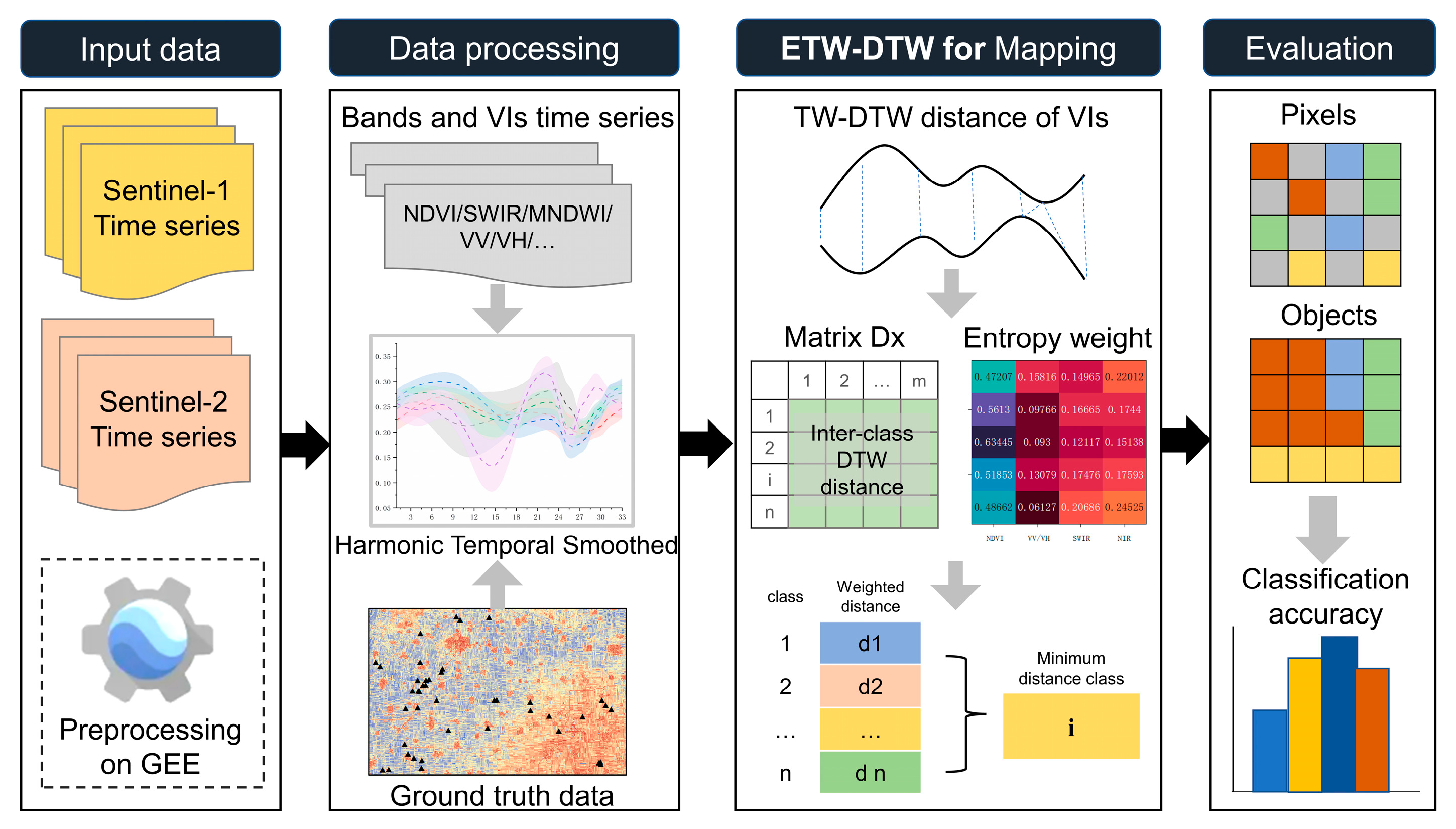
3.3.3. Mapping Fruit-Tree Plantation Using ETW-DTW Method

The minimum distance method is a commonly used approach for determining categories in classification methods based on DTW theory. In this study, due to the introduction of multi-band temporal information, we proposed a minimum distance classification method based on the entropy weight matrix (Section 3.3.2) that enhanced inter-class separability. The workflow is shown in Figure 5. Firstly, for any X to be classified on the dataset, Matrix $D_X$ can be obtained by calculating by row. Line i records the TWDTW distances between the j-sequence curve of class i as the reference and the j-sequence features of x to be classified, respectively. Rows 1 to the n represent the i class as the standard, such as apples, peaches, etc., and columns 1 to m represent various timing features, such as NDVI, NIR, etc. Secondly, based on each category, the weighted distance values $d_i$ of the ith row and m features are calculated. $d_i$ is calculated according to Equation (16), which is the sum of each element in the ith row of the distance matrix and the corresponding entropy weight:

$$d_i=\sum _{j=1}^m(D{x}_{i, j}\times W_j^i)$$

(16)

where $W_j^i$ is the entropy weight of the features obtained in Section 3.3.2, $D{x}_{i, j}$ is the TWDTW distance of j timing curves between X and reference I, and the number of features and categories are m and n, respectively.

Among the n $d_i$ obtained, the class attribute of the X to be classified, $T_X$, is the minimum value of $d_i$:

$$T_X=\mathit{argmin}(d_i)$$

(17)

3.4. Classification Based on Parcel

For the classification of remote sensing images, the most commonly used method is based on the pixel scale. However, it does not utilize the neighborhood information between images, especially for SAR images polluted by speckle noise [74]. To verify the impact of the classification scale on the results, we applied the proposed approach at both pixel and parcel scales. For the pixel basis, the X to be classified is each pixel in the temporal remote sensing images. For the parcel basis, the easiest way is to use a spatial filter [75], such as a mode filter or majority voting. Another approach is to combine it with spatial additional information. Hence, we had two options, called P1 and P2. P1 used the parcel boundaries that we obtained manually on 2020 Google Earth images and the results of pixel classification assigned the parcel to the class with the maximum number of pixels in the parcel. In P2, temporal optical and SAR features were averaged over the polygon based on boundaries (obtained from the 2020 Google earth image manually), and the SITS of the average plot was taken as the minimum unit of classification.

3.5. Accuracy Evaluation

In order to evaluate the accuracy of spatial mapping of the target categories, the most commonly used four indicators, Overall Accuracy (OA), Kappa Coefficient (Kappa Coefficient), Producer Accuracy (PA) and User Accuracy (UA) [76], were selected to evaluate the classification accuracy. The OA and Kappa values are both between 0–1. The closer the value is to 1, the higher the accuracy of the distribution extraction. PA and UA represent the classification accuracy of a single category, and the larger the value, the higher the classification accuracy. Also, the F1-score is used to measure the accuracy of the model. It is the harmonic mean of precision and recall, where precision is the ratio of true positives to all positives, and recall is the ratio of true positives to all actual positives. The F1-score is a better measure of model accuracy than either precision or recall alone, as it takes both into account.

4. Results

4.1. Results of Preprocessing

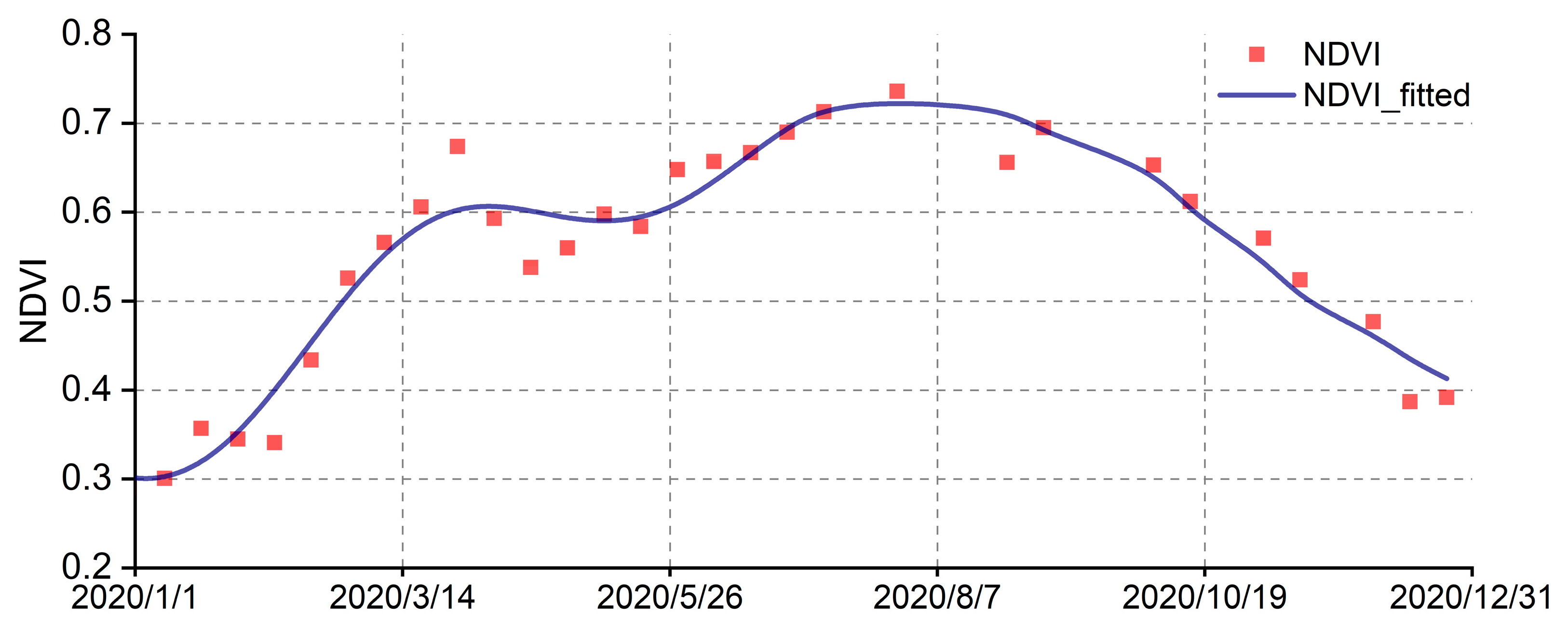
4.1.1. HANTS Simulation of the Time Series Images

As description in article [77], three parameters including the number of frequencies, a high/low suppressions flag and a valid data range were set in the HANTS analysis. The number of frequencies was set to be 1, as the annual scale. The high/low suppressions flag was set to low, considering the cloud and snow contamination led to a low value on the images. The valid data range was set according to different feature characteristics. The HANTS model was applied to every pixel of the S1/2 time series of 2020. An example (NDVI) of the HANTS fitted result and origin time profile is show in Figure 6. The red points are the original values of the NDVI temporal profile, and the HANTS fitted curve is depicted by the bule line. The simulation results demonstrated that HANTS could fit the vegetation index time curve well even in the presence of noticeable data gaps.

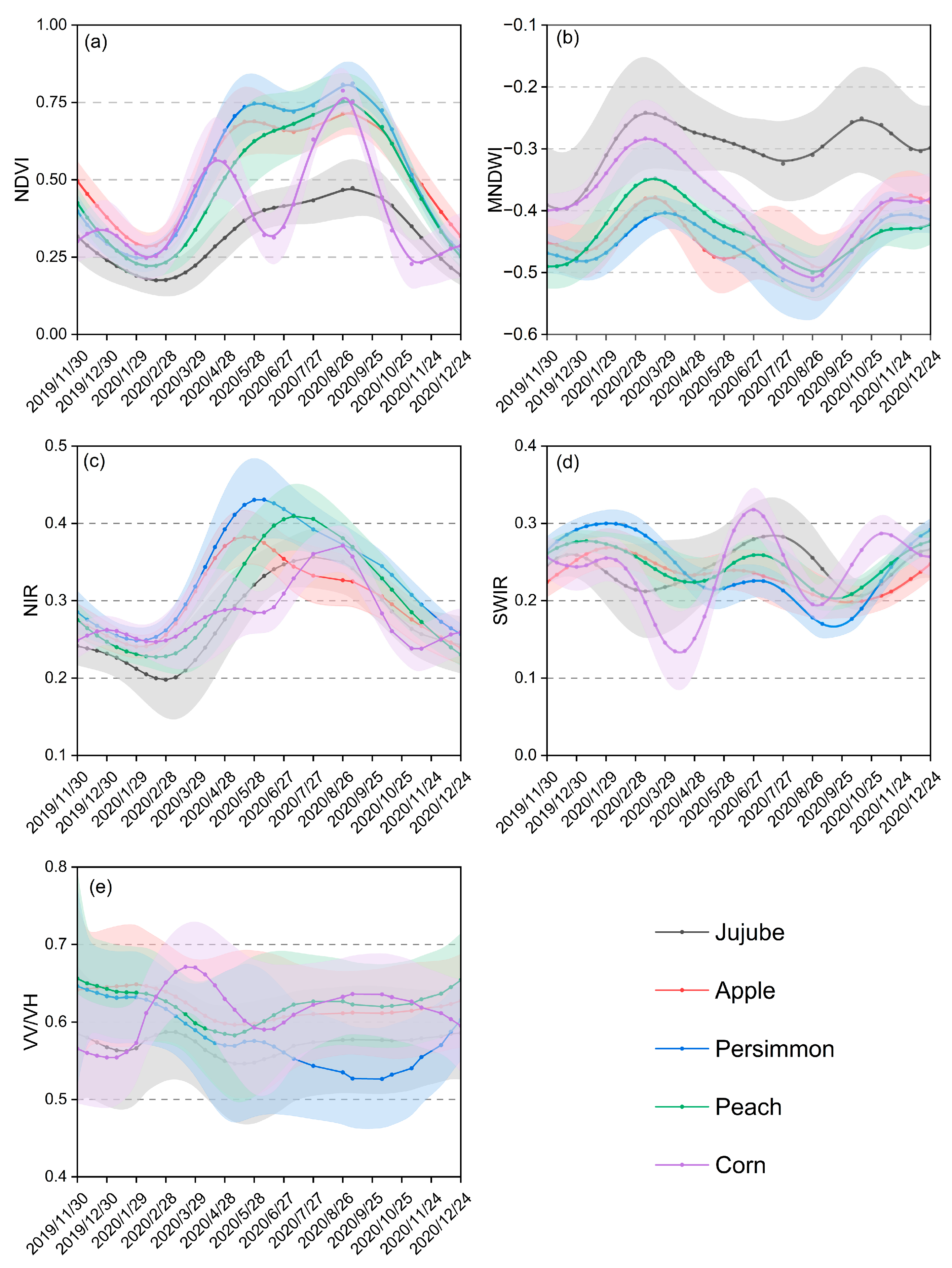
4.1.2. Feature Reduction

On the training set, a two-step approach, as described in Section 3.2, was employed for the temporal index of each class sample, conducting correlation and importance analyses. The results are illustrated in Figure 7. The results showed that three SAR indices, namely VV + VH, VV, and VH, which were ranked low in importance in each period (Figure 7f), were excluded. The correlation matrix [67], calculated using the reference time series curves of each class and each feature, is shown in Figure 7a–e. RVI, EVI, GCVI, GREEN were removed as they were more related to others. Finally, five time series indices, including NDVI, MNDWI, NIR, SWIR, VV/VH, were retained as classification features.

Time series curves depicting NDVI, MNDWI, NIR, SWIR, and VV/VH for jujubes, apples, persimmons, peaches, and corn are presented in Figure 8. Corn, being a food crop, exhibited distinct phenological differences compared to fruit trees, notably evident in the NDVI time series curve (Figure 8a). For the remaining horticultural crops, including jujubes, apples, persimmons and peaches, the time series curves for each optical and SAR index exhibit a remarkably similar shape. This similarity in the temporal patterns poses a challenge for our refined orchard classification, making it more difficult to distinguish between these horticultural crops based solely on the available single index. According to field investigations, in Miaoshang Township, Linyi County, it was observed that the cultivation of jujubes predominantly follows the “greenhouse planting management technology.” The use of jujube tree buckle sheds plays a significant role in reducing natural fertilizer loss, maintaining the ground temperature, accelerating sap flow, and facilitating precise water and fertilizer management as well as yield control. The implementation of buckle sheds resulted in distinctive spectral differences between jujube trees and other fruit trees. In the MNDWI curves (Figure 8b), lower values correspond to higher water content. The regions covered by the plastic film exhibited a lower water content. Conversely, other fruit trees in the natural environment, influenced by the canopy and soil water content, showed relatively high MNDWI values. This difference enhanced the separability between jujubes and other fruit trees.

NIR is related to temperature and moisture. It can be observed (Figure 8c) that in May 2020, the apple curve led by reaching a peak of 0.38, while peaches reached a peak close to 0.40 in July and entered the defoliation period in late October. The slope of the peach curve was significantly higher than that of the apple curve, providing a theoretical basis for the classification of apples and other categories. Persimmons exhibited distinctive wave patterns on the short-wave infrared (SWIR) (Figure 8d) that were quite different from those of the other categories. From early January to mid-February 2020, the patterns showed a continuous upward trend, reaching a peak close to 0.30, significantly higher than the other classes. Subsequently, there was a decline to a minimum value in May 2020, followed by a slight rise to a second peak of 0.23. During this time, the value was lower than for the other types of fruit trees. Afterward, the value dropped sharply to around 0.17 in September 2020, consistently smaller than the other fruit types. Between May and October, the short-wave infrared reflectivity of persimmon orchards remained lower than that of other orchards. The strong absorption of water by short-wave infrared indicates that the water content of persimmon trees during the growth period was higher than that of other orchards.

4.2. The Results of Classification

4.2.1. Entropy Weight Matrix

The key to constructing the ETW-DTW classification method was to select a subset of the classification features and determine the corresponding weight coefficient. In this study, the entropy weight method was employed to quantify the TW-DTW distance weight coefficients of NDVI, MNDWI, NIR, SWIR and VV/VH. A combined classification model was then constructed to classify the fruit trees. Figure 9 displays the results of the entropy matrix, where the horizontal axis represents the five classification features and the ordinate shows the four types of fruit trees. The matrix indicates the weight of each time series index when the four types of orchards are used as the standard. From Figure 9, it was evident that MNDWI had the largest weight in the classification of most crops, particularly in peach classification, with a value of 0.367. NIR exerted the highest impact on jujube classification, with a value of 0.305. NDVI and SWIR contributed similar weights among the target categories, with an average value of 0.207. SAR data contributed to the classification model, with the VV/VH index weights for jujube, persimmon, peach, and apple being 0.145, 0.0672, 0.104, and 0.0915, respectively.

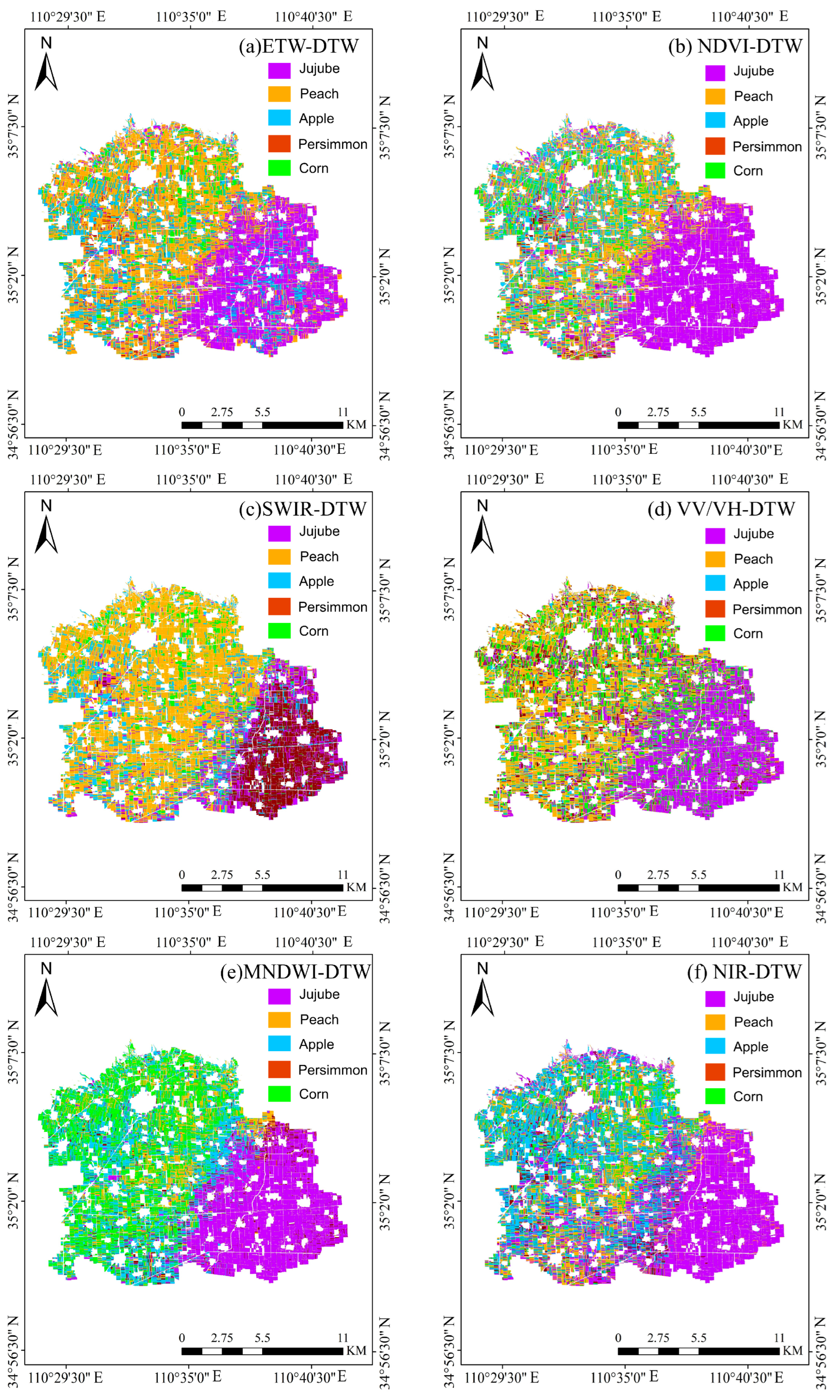
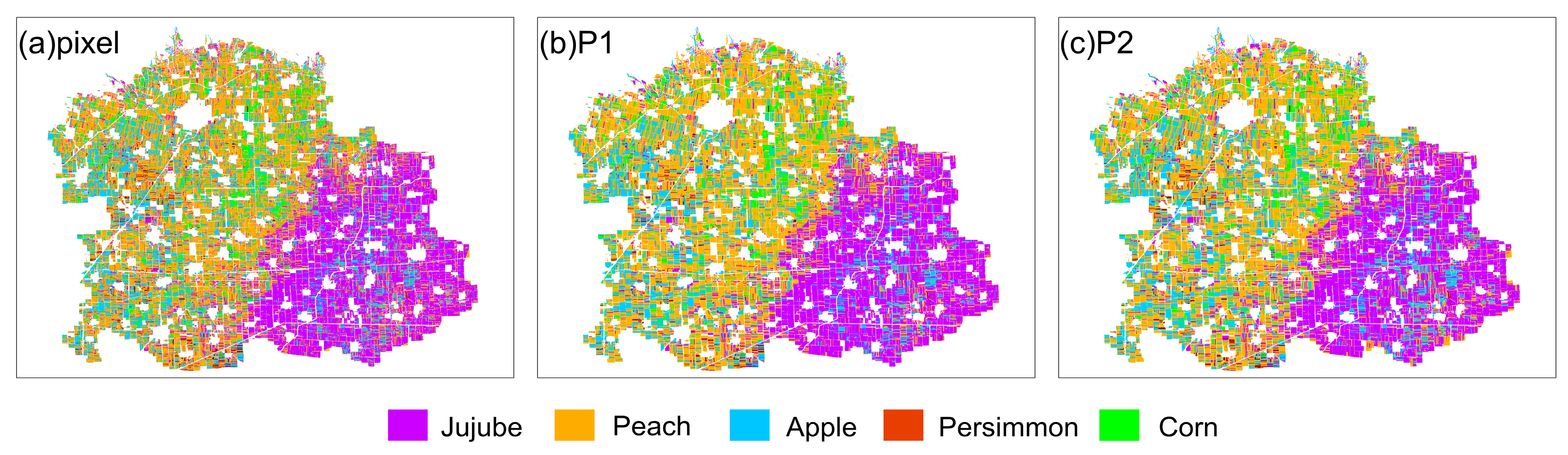
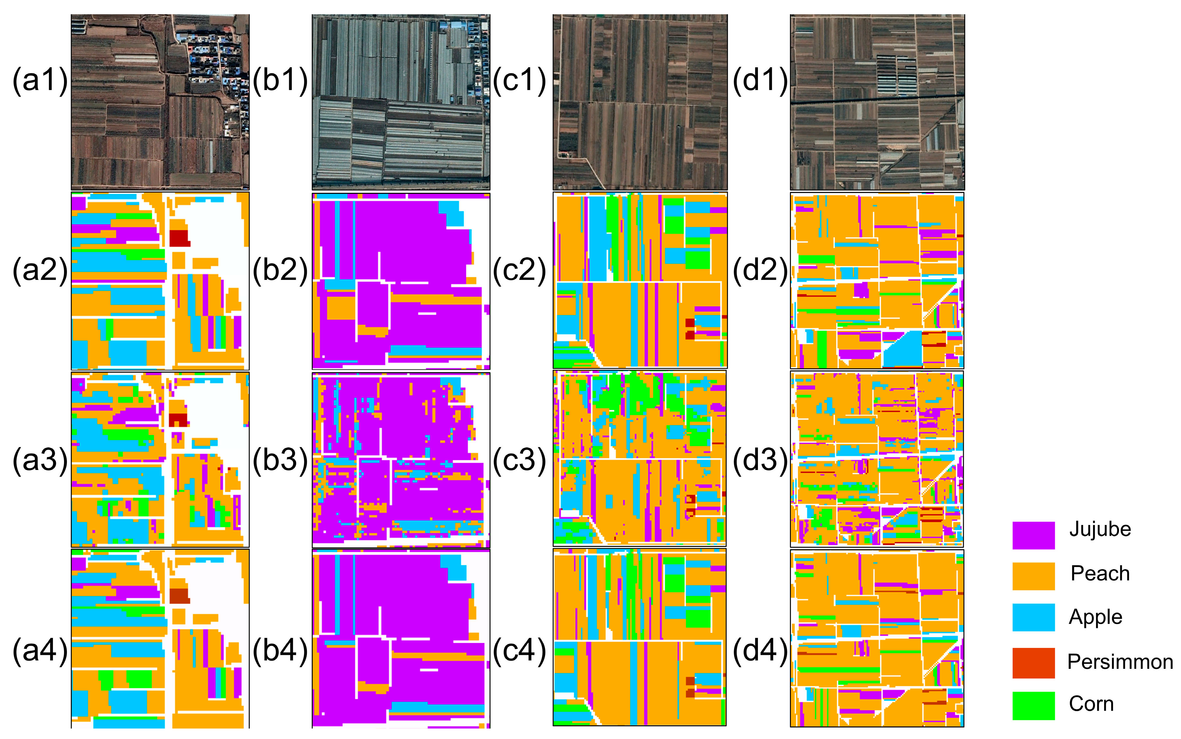
4.2.2. Mapping Orchard Distribution

Using the aforementioned weight matrix, ETW-DTW distances were computed for each pixel/plot. The orchard distribution map (Figure 10a) was then generated employing the minimum distance classification principle (Section 3.3.3). To validate the fine orchard classification model proposed in this paper, we utilized a plot-scale validation set to calculate the accuracy of each fruit tree class. UA, PA, OA, Kappa coefficients, and F1-Score were computed to evaluate the model’s performance. Simultaneously, the classification results with a single time series (NDVI, MNDWI, NIR, SWIR, and VV/VH) were compared. The classification results and accuracy evaluations are presented in Figure 10 and

Table 2. Comparison of extraction accuracy of various crops.

Method	ETW-DTW		NDVI		MNDWI		NIR		SWIR		VV/VH
Class	PA	UA	PA	UA	PA	UA	PA	UA	PA	UA	PA	UA
Jujube	0.932	0.854	0.852	0.937	0.921	0.916	0.763	0.767	0.843	0.495	0.832	0.796
Persimmon	0.509	0.549	0.088	0.212	0.075	0.425	0.137	0.176	0.363	0.436	0.064	0.221
Apple	0.820	0.626	0.743	0.454	0.553	0.377	0.628	0.621	0.712	0.472	0.495	0.112
Peach	0.467	0.710	0.428	0.505	0.514	0.202	0.511	0.475	0.376	0.757	0.316	0.539
OA	0.721		0.643		0.557		0.609		0.544		0.453
KAPPA	0.654		0.580		0.486		0.505		0.403		0.364
F1-score	0.673		0.511		0.446		0.509		0.523		0.374

, respectively. As depicted in Figure 10a, the proposed ETW-DTW fine orchard classification model yielded the best classification results. Table 2 reveals that the overall accuracy (OA) of the ETW-DTW algorithm for each category was 0.721, the Kappa coefficient was 0.654 and the F1-Score was 0.673. Within each fruit tree category, jujube attained the highest user accuracy and producer accuracy of 0.932 and 0.854. The TWDTW classification result of one-dimensional input (NDVI) is shown in Figure 10b. Table 2 indicates that its overall accuracy (OA), Kappa, and F1-Score were 0.643, 0.580, and 0.511, respectively. When NIR was the input (Figure 10f), the OA was 0.609, which was second only to NDVI. However, when SWIR and MNDWI were used as inputs, the overall accuracy was lower, around 0.50, and the Kappa coefficients were less than 0.5. For the VV/VH input, the OA, Kappa coefficients, and F1-Score were the lowest. Therefore, we believe that one-dimensional input does not have an advantage in multi-classification. This type of method can efficiently identify curves that are most different from other categories, but it is challenging to achieve ideal results in multi-class classification with high similarity.

The multi-dimensional input (five optical and SAR indices) provided more favorable classification features, and the weighting amplified the contribution rate of the important indices. The ETW-DTW classification method used multiple features for classification, and the results (Table 2) also showed balanced accuracy results (UA and PA) for various types. The overall classification accuracy was higher than that of the one-dimensional input DTW algorithm. Therefore, ETW-DTW demonstrated the capability to address the multi-classification problem of highly similar phenological features by leveraging the advantages of each index.

4.2.3. Comparison of the Results of the Pixel Scale and Parcel Scale with Two Strategies

In this section, we investigated how the pixel scale and parcel scale affect accuracy. Figure 11 displays the distribution results of horticultural crops by the ETW-DTW model in Miaoshang Township, Qijiao Town, and Linjin Town at the pixel, P1, and P2 scales (described in Section 3.4).

Table 3. Accuracy results of pixel scale classification.

Methods	ETW-DTW-Pixel		ETW-DTW-P1		ETW-DTW-P2
Class	UA	PA	UA	PA	UA	PA
Jujube	0.897	0.841	0.924	0.879	0.932	0.854
Persimmon	0.354	0.399	0.444	0.457	0.509	0.549
Apple	0.752	0.489	0.799	0.518	0.820	0.626
Peach	0.399	0.667	0.443	0.746	0.467	0.710
OA	0.648		0.692		0.721
KAPPA	0.567		0.621		0.654
F1-score	0.584		0.634		0.673

shows the accuracy evaluation on the pixel scale (ETW-DTW-pixel) and parcel scales P1 (ETW-DTW-P1) and P2 (ETW-DTW-P2).

Within the scope of the study area, four areas, such as near buildings, greenhouse areas, farmland areas and roads, were selected for local magnification for further analysis. As shown in Figure 12, the first row Figure 12(a1–d1) displays the Google image of these four areas, the second row Figure 12(a2–d2) displays the P1-based classification results, the third row Figure 12(a3–d3) displays the classification results based on the pixel scale, and the 4th row Figure 12(a4–d4) displays the classification results based on P2. Comparing the second row with the third and fourth rows, it can be observed that the boundary of the classification results based on the plot scale is clear, while the pixel scale exhibits noticeable salt and pepper noise. In Figure 12(a1–a4) were the scene near the building, and both results exhibited a certain spatial consistency. However, in the pixel-scale results, there were different types of ‘sporadic’ pixels in the same plot, which was inconsistent with the actual planting situation. With a spatial resolution of 10 m, the salt and pepper noise caused by ‘sporadic’ pixels will significantly impact the area statistics results of various classes. In Figure 12(b1–b4), the scenario under the mode of greenhouse planting is depicted. Both pixel-scale and plot-scale results could identify open-planted peaches and apples inter-planted in greenhouses, confirming that the ETW-DTW algorithm was feasible at the pixel scale. In Figure 12(c1–c4), in the complex and fragmented farmland plot scene, the results at the plot scale were seriously misclassified as ‘peach trees’ for other categories, while the pixel scale could avoid large-scale misclassification. In Figure 12(d1–d4), in the scene near the road, there were mixed pixels of road and roadside vegetation. In this type of scenario, the influence of confusing pixels at the boundary was suppressed by averaging all pixels at the plot scale during the calculation process, while severe disturbances were evident in the pixel-scale results. Comprehensive Table 3 shows that the overall accuracy of the ETW-DTW model at the pixel scale is lower than of plot scales. The result of using P1 as the plot classification strategy is not as good as that using P2 as the plot classification strategy. The overall accuracy (OA) is 0.029 smaller, Kappa is 0.033 smaller, and the F1-Score is 0.039 smaller. Since P1 is the result of post-processing at the pixel scale, the errors in pixel-scale classification directly affect the performance of P1. For example, as shown in Figure 12(b2,b4), regional differences between P1 and P2 are observed at the boundaries between greenhouses and open orchards. Similarly, in Figure 12(d2,d4), the same phenomenon is evident at the edges of roads where mixed pixels are present. In pixel conditions, pixel-level time series data were more susceptible to noise interference, and even the same features showed time series curves with large differences. Therefore, in areas with mixed pixels, it is advisable to avoid using pixel-scale or pixel post-processing methods like P1. Instead, a plot-based averaging method such as P2 should be used. When considering averaged plots, the influence is eliminated. The time series curve at the plot scale could reflect the real geophysical characteristics, thereby improving the accuracy of classification.

5. Discussion

5.1. Advantages of the ETW-DTW Method

In this paper, we introduced an ETW-DTW classification method rooted in the TWDTW theory that leverages entropy weighting to integrate multiple attributes. This approach was applied to long time series data from S1/2 imagery to identify orchard distributions characterized by extremely similar phenological features. The accuracy evaluation confirmed the feasibility of the ETW-DTW method for classifying highly similar categories at the pixel scale and plot scale. After analysis, this method has the following advantages.

5.1.1. Integration of SAR Data

Since 2017, the launch of Sentinel-2B has increased the original 10-day revisit period of Sentinel-2 data to 5 days. The enhanced time resolution has led researchers worldwide to favor Sentinel-2 as their primary data source for experiments [40,78,79]. However, optical images are vulnerable to cloud and snow interference, posing challenges in acquiring high-quality datasets for extensive study areas. The participation of SAR data (Sentinel-1) can make up for the spatial limitations of optical images, which can obtain time-series images of day and night and are not easily affected by clouds and rain. SAR imagery has been extensively applied in thematic mapping of land use, demonstrating its high sensitivity in identifying bare soils and crops. Moreover, SAR features exhibit a strong correlation with vegetation structure and phenological characteristics [63]. Recent years have witnessed an increasing focus on research exploring the classification applications stemming from the synergistic use of S1 and S2 data. In this paper, an examination of the importance of ranking results obtained from random forest analysis (Figure 7) and the entropy matrix (Figure 9) underscores the substantial contribution of SAR data to the classification process. Furthermore, Figure 8e revealed notable distinctions in the VV/VH timing curves between corn rotation crops and horticultural crops, affirming the discriminative power of SAR data in capturing diverse waveforms associated with different land cover types.

To further validate the contribution of SAR data in orchard classification, we compared the results obtained by combining S1 and S2 with those using only S2 images. In the S2-only experiment, only four optical data indices were involved in the calculation, and their entropy-weighted weights are shown in Figure 13. It was observed that for jujube classification, the NIR had the highest entropy-weighted weight, and for persimmon, peach, and apple, the MNDWI index had the highest weight. This trend was consistent with the one when SAR data was included (Figure 9).

Table 4. Comparison of Accuracy Between S1/2 and S2 Results.

Methods	ETW-DTW-S2		ETW-DTW-S1/2
Class	UA	PA	UA	PA
Jujube	0.933	0.845	0.932	0.854
Persimmon	0.213	0.263	0.509	0.549
Apple	0.793	0.551	0.820	0.626
Peach	0.419	0.674	0.467	0.710
OA	0.665		0.721
KAPPA	0.586		0.654
F1-score	0.572		0.673

shows the difference in accuracy with or without SAR data. In the classification of the jujube orchard, the difference in accuracy between the two was not significant. For persimmons, the UA increased from 0.213 to 0.509 and the PA increased from 0.263 to 0.549. For apples, the UA increased from 0.793 to 0.820 and the PA increased from 0.551 to 0.626. For peaches, the UA increased from 0.419 to 0.467 and the PA increased from 0.674 to 0.710. In overall accuracy, the inclusion of SAR data resulted in a higher OA/KAPPA and F1-score compared to using only optical indices. In conclusion, the addition of SAR data was advantageous for improving the accuracy of fruit tree classification.

5.1.2. Individual Contributions of ETW-DTW Model

• Advantages of TWDTW algorithm in orchard classification The choice of classifier determines the accuracy of the classification result [80]. In this study, the TWDTW algorithm was deliberately chosen due to its demonstrated efficacy in handling crop classification tasks utilizing time series imagery: (1) when employing vegetation phenological characteristics as the basis for classification, variations in weather conditions and agricultural practices can introduce disparities in the time series curve characteristics for the same crop. The TWDTW algorithm adeptly mitigates such differences by distorting and aligning the two curves [41]; and (2) the classifier’s performance is directly influenced by the number of samples available for training [33]. The TWDTW algorithm stands out as one of the few algorithms that do not demand a high number of samples [81]. As long as the standard curve adheres to the temporal pattern characteristics of the target category, ideal accuracy can be achieved [44]. Belgiu and Csillik [40] compared the accuracy of the DTW algorithm and the random forest algorithm under small samples to confirm this view.
• The strengths of the entropy weight matrix In this experiment, we attempted to employ the entropy weight method to assign weights to multiple indices, aiming to enable the input of the TWDTW algorithm for multi-dimensional curves and enhance the accuracy of the results. As shown in Table 2, compared to the traditional single-band TWDTW method, the ETW-DTW method, which integrates multi-band information, demonstrates significant advantages. According to the principle of entropy weighting, the level of information entropy depends on the probability distribution of the data, making it highly robust to outliers. In contrast, the variance weighting method also assigns weights based on data dispersion but is highly sensitive to outliers and performs poorly when the indices have different scales or the data characteristics are not distinct. Using the same approach, we replaced the entropy weights with variance weights to obtain the classification accuracy for orchard classification. The overall accuracy (OA) was 0.627, the Kappa coefficient was 0.494, and the F1-score was 0.593, all of which are lower than the classification accuracy based on entropy weights. Overall, entropy weighting better reflects the relative information content of each index, reduces the impact of outliers and extreme values, and is more suitable for handling complex ecological analysis problems involving multiple indices, scales, and distributions.

5.1.3. The Generalizability of ETW-DTW

Although the ETW-DTW method has achieved reasonable accuracy within the current study area, the generalizability of the classification method remains a topic worth exploring. Here, we discuss the advantages of the ETW-DTW method in classification from two perspectives: geographic transferability and class transferability.

In this study, logistic TWDTW was used to calculate the optimal path length between two curves. Compared to linear TWDTW, logistic TWDTW offers higher classification sensitivity [42] because it heavily penalizes large temporal warping. When analyzing the same type of crops in different geographic locations, due to differences in climate and agricultural practices, the phenological characteristics of the same crops may show similar trends but be asynchronous. TWDTW can effectively align the peaks and troughs of two time series curves through optimal path search, thereby minimizing intra-class errors in phenological curves of the same crop caused by temporal asynchrony. Additionally, the availability of high-quality remote sensing images varies across different geographic regions. In large-scale studies, the inconsistency in the number of time-series images between the sample areas and the regions to be classified is one of the major reasons for suboptimal classification results. Fortunately, TWDTW, initially used for speech recognition, is one of the few methods capable of determining the similarity of time series of different lengths. In time-series remote sensing analysis, TWDTW can mitigate classification errors caused by differences in image availability and has the potential to extract target classes over large areas.

For orchard classification involving different types of fruit trees, the lack of sufficient samples prevents us from validating the accuracy of the trained ETW-DTW model for other types of fruit tree classifications. However, in theory, the core of the ETW-DTW model lies in utilizing entropy theory, where the dispersion of the TWDTW distance set is used as a measure of separability between classes. In this process, the determination of weights is a completely data-driven method, without the subjective participation of the experimenter (the obtained entropy weight results depend on the phenological characteristics of each target class). In theory, the method framework is transferable to other categories.

5.2. Limitations of the ETW-DTW Method

During the experiment, we found some algorithm limitations and areas for improvement. We utilized the ETW-DTW distance to assess class confusions, identifying instances where time series patterns differed from the reference patterns. It has been demonstrated that DTW dissimilarity can be a valuable resource for understanding the spatio-temporal autocorrelation of time series images [39]. However, the DTW algorithm exhibited weak resistance to intra-class variability. Throughout this process, we made the assumption that the difference between categories (inter-class difference) was greater than the difference within the category itself (intra-class difference). However, variations in the planting structure and pattern of fruit trees introduced heterogeneity within the same class, thereby impacting classification accuracy. Intra-class heterogeneity is a contributing factor to the lower classification accuracy of the DTW algorithm compared to machine learning algorithms under conditions of sufficient samples. This limitation may hinder the model from achieving optimal results on a large scale. Although it can mitigate the effects of phenological delays and advances in fruit trees, the heterogeneity caused by different varieties and planting structures within the same type of fruit tree is a non-negligible issue. Therefore, in further efforts to implement orchard classification at national or global scales, suppressing intra-class errors within the same category is a gap that the current version of the ETW-DTW model needs to address. Further research is necessary to explore the significance of the ETW-DTW in measuring spatiotemporal autocorrelation and mitigating intra-class differences. We believe that incorporating an intra-class variability suppression module into the ETW-DTW model would greatly enhance its potential for large-scale classification projects.

6. Conclusions

Utilizing Sentinel-1/2 time series image data, this study introduces a novel classification approach based on the Time-Weighted Dynamic Time Warping (TWDTW) theory and entropy weight theory (ETW-DTW) at the plot scale for orchard class delineation. Building upon the traditional TWDTW algorithm, which outputs single-band results, the ETW-DTW method innovatively integrates multi-attribute time-series data through entropy-weighted theory, achieving an overall improvement in classification accuracy. This approach was applied in three counties in Shanxi Province, China, and yielded satisfactory results for orchard classification, where phenological and structural similarities are high. The ETW-DTW method has a very low dependency on sample size, making it an ideal choice for large-scale agricultural surveys where sufficient sample collection is challenging due to harsh environmental conditions. The successful implementation of this workflow has the potential to enhance the efficiency of cash crop production, ensuring a sustainable agricultural and forestry environment. Additionally, the ETW-DTW method holds potential value for sample augmentation tasks and is of great significance for monitoring cropping systems, assessing crop growth conditions, estimating yields, and characterizing land ecosystem dynamics.

References

1. Yuan, B.; Yue, F.; Cui, Y.; Chen, C. The role of fine management techniques in relation to agricultural pollution and farmer income: The case of the fruit industry. Environ. Res. Lett. 2022, 17, 034001. [Google Scholar] [CrossRef]
2. Massey, R.; Sankey, T.T.; Congalton, R.G.; Yadav, K.; Thenkabail, P.S.; Ozdogan, M.; Meador, A.J.S. MODIS phenology-derived, multi-year distribution of conterminous US crop types. Remote Sens. Environ. 2017, 198, 490–503. [Google Scholar] [CrossRef]
3. Abbasi, N.; Nouri, H.; Didan, K.; Barreto-Muñoz, A.; Chavoshi Borujeni, S.; Salemi, H.; Opp, C.; Siebert, S.; Nagler, P.J.R.S. Estimating actual evapotranspiration over croplands using vegetation index methods and dynamic harvested area. Remote Sens. 2021, 13, 5167. [Google Scholar] [CrossRef]
4. Berni, J.; Zarco-Tejada, P.; Sepulcre-Cantó, G.; Fereres, E.; Villalobos, F. Mapping canopy conductance and CWSI in olive orchards using high resolution thermal remote sensing imagery. Remote Sens. Environ. 2009, 113, 2380–2388. [Google Scholar] [CrossRef]
5. French, A.N.; Hunsaker, D.J.; Sanchez, C.A.; Saber, M.; Gonzalez, J.R.; Anderson, R.J.A.W.M. Satellite-based NDVI crop coefficients and evapotranspiration with eddy covariance validation for multiple durum wheat fields in the US Southwest. Agric. Water Manag. 2020, 239, 106266. [Google Scholar] [CrossRef]
6. Lhermitte, S.; Verbesselt, J.; Verstraeten, W.W.; Coppin, P. A comparison of time series similarity measures for classification and change detection of ecosystem dynamics. Remote Sens. Environ. 2011, 115, 3129–3152. [Google Scholar] [CrossRef]
7. Jin, S.; Sader, S.A. MODIS time-series imagery for forest disturbance detection and quantification of patch size effects. Remote Sens. Environ. 2005, 99, 462–470. [Google Scholar] [CrossRef]
8. Linderman, M.; Rowhani, P.; Benz, D.; Serneels, S.; Lambin, E.F. Land-cover change and vegetation dynamics across Africa. J. Geophys. Res. Atmos. 2005, 110, 12104. [Google Scholar] [CrossRef]
9. Zhang, X.; Friedl, M.A.; Schaaf, C.B. Global vegetation phenology from Moderate Resolution Imaging Spectroradiometer (MODIS): Evaluation of global patterns and comparison with in situ measurements. J. Geophys. Res. Biogeosci. 2006, 111, 367–375. [Google Scholar] [CrossRef]
10. Weiss, M.; Jacob, F.; Duveiller, G. Remote sensing for agricultural applications: A meta-review. Remote Sens. Environ. 2020, 236, 111402. [Google Scholar] [CrossRef]
11. Waldner, F.; Fritz, S.; Di Gregorio, A.; Defourny, P. Mapping priorities to focus cropland mapping activities: Fitness assessment of existing global, regional and national cropland maps. Remote Sens. 2015, 7, 7959–7986. [Google Scholar] [CrossRef]
12. Cai, Y.; Guan, K.; Peng, J.; Wang, S.; Seifert, C.; Wardlow, B.; Li, Z. A high-performance and in-season classification system of field-level crop types using time-series Landsat data and a machine learning approach. Remote Sens. Environ. 2018, 210, 35–47. [Google Scholar] [CrossRef]
13. Fu, G.; Liu, C.; Zhou, R.; Sun, T.; Zhang, Q. Classification for high resolution remote sensing imagery using a fully convolutional network. Remote Sens. 2017, 9, 498. [Google Scholar] [CrossRef]
14. Delrue, J.; Bydekerke, L.; Eerens, H.; Gilliams, S.; Piccard, I.; Swinnen, E. Crop mapping in countries with small-scale farming: A case study for West Shewa, Ethiopia. Int. J. Remote Sens. 2013, 34, 2566–2582. [Google Scholar] [CrossRef]
15. Gella, G.W. Mapping Crop Types in Smallholder Farming Areas using SAR Imagery with Dynamic Time Warping. Master’s Thesis, University of Twente, Enschede, The Netherlands, 2020. [Google Scholar]
16. Xu, D.; Guo, X. Compare NDVI extracted from Landsat 8 imagery with that from Landsat 7 imagery. Am. J. Remote Sens. 2014, 2, 10–14. [Google Scholar] [CrossRef]
17. Pan, Z.; Huang, J.; Zhou, Q.; Wang, L.; Cheng, Y.; Zhang, H.; Blackburn, G.A.; Yan, J.; Liu, J. Mapping crop phenology using NDVI time-series derived from HJ-1 A/B data. Int. J. Appl. Earth Obs. Geoinf. 2015, 34, 188–197. [Google Scholar] [CrossRef]
18. El Hajj, M.; Bégué, A.; Guillaume, S.; Martiné, J.-F. Integrating SPOT-5 time series, crop growth modeling and expert knowledge for monitoring agricultural practices—The case of sugarcane harvest on Reunion Island. Remote Sens. Environ. 2009, 113, 2052–2061. [Google Scholar] [CrossRef]
19. Murakami, T.; Ogawa, S.; Ishitsuka, N.; Kumagai, K.; Saito, G. Crop discrimination with multitemporal SPOT/HRV data in the Saga Plains, Japan. Int. J. Remote Sens. 2001, 22, 1335–1348. [Google Scholar] [CrossRef]
20. McNairn, H.; Brisco, B. The application of C-band polarimetric SAR for agriculture: A review. Can. J. Remote Sens. 2004, 30, 525–542. [Google Scholar] [CrossRef]
21. Khabbazan, S.; Vermunt, P.; Steele-Dunne, S.; Ratering Arntz, L.; Marinetti, C.; van der Valk, D.; Iannini, L.; Molijn, R.; Westerdijk, K.; van der Sande, C. Crop monitoring using Sentinel-1 data: A case study from The Netherlands. Remote Sens. 2019, 11, 1887. [Google Scholar] [CrossRef]
22. Xie, G.; Niculescu, S.J.R.S. Mapping crop types using sentinel-2 data machine learning and monitoring crop phenology with sentinel-1 backscatter time series in pays de Brest, Brittany, France. Remote Sens. 2022, 14, 4437. [Google Scholar] [CrossRef]
23. Danilla, C.; Persello, C.; Tolpekin, V.; Bergado, J.R. Classification of multitemporal SAR images using convolutional neural networks and Markov random fields. In Proceedings of the 2017 IEEE International Geoscience and Remote Sensing Symposium (IGARSS), Fort Worth, TX, USA, 23–28 July 2017; pp. 2231–2234. [Google Scholar]
24. Niculescu Sr, S.; Billey, A.; Talab-Ou-Ali, H., Jr. Random forest classification using Sentinel-1 and Sentinel-2 series for vegetation monitoring in the Pays de Brest (France). In Proceedings of the Remote Sensing for Agriculture, Ecosystems, and Hydrology XX, Berlin, Germany, 10–13 September 2018; p. 1078305. [Google Scholar]
25. Betbeder, J.; Laslier, M.; Corpetti, T.; Pottier, E.; Corgne, S.; Hubert-Moy, L. Multi-temporal optical and radar data fusion for crop monitoring: Application to an intensive agricultural area in Brittany (France). In Proceedings of the 2014 IEEE Geoscience and Remote Sensing Symposium, Quebec City, QC, Canada, 13–18 July 2014; pp. 1493–1496. [Google Scholar]
26. Dusseux, P.; Corpetti, T.; Hubert-Moy, L.; Corgne, S. Combined use of multi-temporal optical and radar satellite images for grassland monitoring. Remote Sens. 2014, 6, 6163–6182. [Google Scholar] [CrossRef]
27. Colson, D.; Petropoulos, G.P.; Ferentinos, K.P. Exploring the potential of Sentinels-1 & 2 of the Copernicus Mission in support of rapid and cost-effective wildfire assessment. Int. J. Appl. Earth Obs. Geoinf. 2018, 73, 262–276. [Google Scholar]
28. Rajah, P.; Odindi, J.; Mutanga, O. Feature level image fusion of optical imagery and Synthetic Aperture Radar (SAR) for invasive alien plant species detection and mapping. Remote Sens. Appl. Soc. Environ. 2018, 10, 198–208. [Google Scholar] [CrossRef]
29. Skriver, H. Crop classification by multitemporal C-and L-band single-and dual-polarization and fully polarimetric SAR. IEEE Trans. Geosci. Remote Sens. 2011, 50, 2138–2149. [Google Scholar] [CrossRef]
30. Huang, X.; Wang, J.; Shang, J.; Liao, C.; Liu, J. Application of polarization signature to land cover scattering mechanism analysis and classification using multi-temporal C-band polarimetric RADARSAT-2 imagery. Remote Sens. Environ. 2017, 193, 11–28. [Google Scholar] [CrossRef]
31. Waske, B.; Braun, M. Classifier ensembles for land cover mapping using multitemporal SAR imagery. ISPRS J. Photogramm. Remote Sens. 2009, 64, 450–457. [Google Scholar] [CrossRef]
32. Sonobe, R.; Tani, H.; Wang, X.; Kobayashi, N.; Shimamura, H. Discrimination of crop types with TerraSAR-X-derived information. Phys. Chem. Earth Parts A/B/C 2015, 83, 2–13. [Google Scholar] [CrossRef]
33. Gao, H.; Wang, C.; Wang, G.; Fu, H.; Zhu, J. A novel crop classification method based on ppfSVM classifier with time-series alignment kernel from dual-polarization SAR datasets. Remote Sens. Environ. 2021, 264, 112628. [Google Scholar] [CrossRef]
34. Zhong, L.; Hu, L.; Yu, L.; Gong, P.; Biging, G.S. Automated mapping of soybean and corn using phenology. ISPRS J. Photogramm. Remote Sens. 2016, 119, 151–164. [Google Scholar] [CrossRef]
35. Waldner, F.; Canto, G.S.; Defourny, P. Automated annual cropland mapping using knowledge-based temporal features. ISPRS J. Photogramm. Remote Sens. 2015, 110, 1–13. [Google Scholar] [CrossRef]
36. Bargiel, D. A new method for crop classification combining time series of radar images and crop phenology information. Remote Sens. Environ. 2017, 198, 369–383. [Google Scholar] [CrossRef]
37. Kenduiywo, B.K.; Bargiel, D.; Soergel, U. Higher order dynamic conditional random fields ensemble for crop type classification in radar images. IEEE Trans. Geosci. Remote Sens. 2017, 55, 4638–4654. [Google Scholar] [CrossRef]
38. Leite, P.B.C.; Feitosa, R.Q.; Formaggio, A.R.; da Costa, G.A.O.P.; Pakzad, K.; Sanches, I.D.A. Hidden Markov Models for crop recognition in remote sensing image sequences. Pattern Recognit. Lett. 2011, 32, 19–26. [Google Scholar] [CrossRef]
39. Csillik, O.; Belgiu, M.; Asner, G.P.; Kelly, M. Object-based time-constrained dynamic time warping classification of crops using Sentinel-2. Remote Sens. 2019, 11, 1257. [Google Scholar] [CrossRef]
40. Belgiu, M.; Csillik, O. Sentinel-2 cropland mapping using pixel-based and object-based time-weighted dynamic time warping analysis. Remote Sens. Environ. 2018, 204, 509–523. [Google Scholar] [CrossRef]
41. Petitjean, F.; Inglada, J.; Gançarski, P. Satellite image time series analysis under time warping. IEEE Trans. Geosci. Remote Sens. 2012, 50, 3081–3095. [Google Scholar] [CrossRef]
42. Maus, V.; Câmara, G.; Cartaxo, R.; Sanchez, A.; Ramos, F.M.; De Queiroz, G.R. A time-weighted dynamic time warping method for land-use and land-cover mapping. IEEE J. Sel. Top. Appl. Earth Obs. Remote Sens. 2016, 9, 3729–3739. [Google Scholar] [CrossRef]
43. Xu, H.; Qi, S.; Gong, P.; Liu, C.; Wang, J. Long-term monitoring of citrus orchard dynamics using time-series Landsat data: A case study in southern China. Int. J. Remote Sens. 2018, 39, 8271–8292. [Google Scholar] [CrossRef]
44. Dong, Q.; Chen, X.; Chen, J.; Zhang, C.; Liu, L.; Cao, X.; Zang, Y.; Zhu, X.; Cui, X. Mapping winter wheat in North China using Sentinel 2A/B data: A method based on phenology-time weighted dynamic time warping. Remote Sens. 2020, 12, 1274. [Google Scholar] [CrossRef]
45. Gella, G.W.; Bijker, W.; Belgiu, M. Mapping crop types in complex farming areas using SAR imagery with dynamic time warping. ISPRS J. Photogramm. Remote Sens. 2021, 175, 171–183. [Google Scholar] [CrossRef]
46. Fagan, M.E.; DeFries, R.S.; Sesnie, S.E.; Arroyo-Mora, J.P.; Soto, C.; Singh, A.; Townsend, P.A.; Chazdon, R.L.J.R.S. Mapping species composition of forests and tree plantations in Northeastern Costa Rica with an integration of hyperspectral and multitemporal Landsat imagery. Remote Sens. 2015, 7, 5660–5696. [Google Scholar] [CrossRef]
47. Xiao, C.; Li, P.; Feng, Z.; Liu, Y.; Zhang, X. Geoinformation, Sentinel-2 red-edge spectral indices (RESI) suitability for mapping rubber boom in Luang Namtha Province, northern Lao PDR. Int. J. Appl. Earth Obs. Geoinf. 2020, 93, 102176. [Google Scholar]
48. Abbasi, M.; Verrelst, J.; Mirzaei, M.; Marofi, S.; Riyahi Bakhtiari, H.R. Optimal spectral wavelengths for discriminating orchard species using multivariate statistical techniques. Remote Sens. 2019, 12, 63. [Google Scholar] [CrossRef] [PubMed]
49. Peña, M.; Liao, R.; Brenning, A. Using spectrotemporal indices to improve the fruit-tree crop classification accuracy. ISPRS J. Photogramm. Remote Sens. 2017, 128, 158–169. [Google Scholar] [CrossRef]
50. Cui, B.; Huang, W.; Ye, H.; Chen, Q. The suitability of PlanetScope imagery for mapping rubber plantations. Remote Sens. 2022, 14, 1061. [Google Scholar] [CrossRef]
51. Nagori, R. Discrimination of mango orchards in Malihabad, India using textural features. Geocarto Int. 2021, 36, 1060–1074. [Google Scholar] [CrossRef]
52. Li, J.; Yang, G.; Yang, H.; Xu, W.; Feng, H.; Xu, B.; Chen, R.; Zhang, C.; Wang, H. Orchard classification based on super-pixels and deep learning with sparse optical images. Comput. Electron. Agric. 2023, 215, 108379. [Google Scholar] [CrossRef]
53. Nabil, M.; Farg, E.; Arafat, S.M.; Aboelghar, M.; Afify, N.M.; Elsharkawy, M.M. Environment, Tree-fruits crop type mapping from Sentinel-1 and Sentinel-2 data integration in Egypt’s New Delta project. Remote Sens.Appl. Soc. Environ. 2022, 27, 100776. [Google Scholar]
54. Kordi, F.; Yousefi, H. Environment, Crop classification based on phenology information by using time series of optical and synthetic-aperture radar images. Remote Sens.Appl. Soc. Environ. 2022, 27, 100812. [Google Scholar]
55. d’Andrimont, R.; Taymans, M.; Lemoine, G.; Ceglar, A.; Yordanov, M.; van der Velde, M. Detecting flowering phenology in oil seed rape parcels with Sentinel-1 and-2 time series. Remote Sens. Environ. 2020, 239, 111660. [Google Scholar] [CrossRef] [PubMed]
56. Griffiths, P.; Nendel, C.; Hostert, P. Intra-annual reflectance composites from Sentinel-2 and Landsat for national-scale crop and land cover mapping. Remote Sens. Environ. 2019, 220, 135–151. [Google Scholar] [CrossRef]
57. Xu, L.; Zhang, H.; Wang, C.; Zhang, B.; Liu, M. Crop classification based on temporal information using sentinel-1 SAR time-series data. Remote Sens. 2018, 11, 53. [Google Scholar] [CrossRef]
58. Lee, J.-S. Digital image smoothing and the sigma filter. Comput. Vis. Graph. Image Process. 1983, 24, 255–269. [Google Scholar] [CrossRef]
59. You, N.; Dong, J.; Huang, J.; Du, G.; Zhang, G.; He, Y.; Yang, T.; Di, Y.; Xiao, X. The 10-m crop type maps in Northeast China during 2017–2019. Sci. Data 2021, 8, 41. [Google Scholar] [CrossRef]
60. Yang, G.; Shen, H.; Zhang, L.; He, Z.; Li, X. A moving weighted harmonic analysis method for reconstructing high-quality SPOT VEGETATION NDVI time-series data. IEEE Trans. Geosci. Remote Sens. 2015, 53, 6008–6021. [Google Scholar] [CrossRef]
61. Xu, Y.; Shen, Y.; Wu, Z. Development, Spatial and temporal variations of land surface temperature over the Tibetan Plateau based on harmonic analysis. Mt. Res. Dev. 2013, 33, 85–94. [Google Scholar] [CrossRef]
62. Peña, M.; Brenning, A. Assessing fruit-tree crop classification from Landsat-8 time series for the Maipo Valley, Chile. Remote Sens. Environ. 2015, 171, 234–244. [Google Scholar] [CrossRef]
63. Denize, J.; Hubert-Moy, L.; Betbeder, J.; Corgne, S.; Baudry, J.; Pottier, E. Evaluation of using sentinel-1 and-2 time-series to identify winter land use in agricultural landscapes. Remote Sens. 2018, 11, 37. [Google Scholar] [CrossRef]
64. Breiman, L. Random forests. Mach. Learn. 2001, 45, 5–32. [Google Scholar] [CrossRef]
65. Kostelich, E.J.; Schreiber, T. Noise reduction in chaotic time-series data: A survey of common methods. Phys. Rev. E 1993, 48, 1752. [Google Scholar] [CrossRef] [PubMed]
66. Pal, M. Random forest classifier for remote sensing classification. Int. J. Remote Sens. 2005, 26, 217–222. [Google Scholar] [CrossRef]
67. Veloso, A.; Mermoz, S.; Bouvet, A.; Le Toan, T.; Planells, M.; Dejoux, J.-F.; Ceschia, E. Understanding the temporal behavior of crops using Sentinel-1 and Sentinel-2-like data for agricultural applications. Remote Sens. Environ. 2017, 199, 415–426. [Google Scholar] [CrossRef]
68. Rakszawski, B.; Wright, R.; Cadieux, J.H.; Davidson, L.S.; Brenner, C. The Effects of Preprocessing Strategies for Pediatric Cochlear Implant Recipients. J. Am. Acad. Audiol. 2016, 27, 85–102. [Google Scholar] [CrossRef]
69. Zhang, Z.; Tang, P.; Huo, L.; Zhou, Z. MODIS NDVI time series clustering under dynamic time warping. Int. J. Wavelets Multiresolut. Inf. Process. 2014, 12, 1461011. [Google Scholar] [CrossRef]
70. Li, F.J.; Ren, J.Q.; Wu, S.R.; Zhao, H.W.; Zhang, N.D. Comparison of Regional Winter Wheat Mapping Results from Different Similarity Measurement Indicators of NDVI Time Series and Their Optimized Thresholds. Remote Sens. 2021, 13, 1162. [Google Scholar] [CrossRef]
71. Peña-Barragán, J.M.; Ngugi, M.K.; Plant, R.E.; Six, J. Object-based crop identification using multiple vegetation indices, textural features and crop phenology. Remote Sens. Environ. 2011, 115, 1301–1316. [Google Scholar] [CrossRef]
72. Fei, S.; Hassan, M.; Ma, Y.; Shu, M.; Cheng, Q.; Li, Z.; Chen, Z.; Xiao, Y. Entropy Weight Ensemble Framework for Yield Prediction of Winter Wheat Under Different Water Stress Treatments Using Unmanned Aerial Vehicle-Based Multispectral and Thermal Data. Front. Plant Sci. 2021, 12, 730181. [Google Scholar] [CrossRef]
73. Farhadinia, B. A multiple criteria decision making model with entropy weight in an interval-transformed hesitant fuzzy environment. Cogn. Comput. 2017, 9, 513–525. [Google Scholar] [CrossRef]
74. Kussul, N.; Lemoine, G.; Gallego, F.J.; Skakun, S.V.; Lavreniuk, M.; Shelestov, A.Y. Parcel-based crop classification in Ukraine using Landsat-8 data and Sentinel-1A data. IEEE J. Sel. Top. Appl. Earth Obs. Remote Sens. 2016, 9, 2500–2508. [Google Scholar] [CrossRef]
75. McNairn, H.; Champagne, C.; Shang, J.; Holmstrom, D.; Reichert, G. Integration of optical and Synthetic Aperture Radar (SAR) imagery for delivering operational annual crop inventories. ISPRS J. Photogramm. Remote Sens. 2009, 64, 434–449. [Google Scholar] [CrossRef]
76. Congalton, R.G. A review of assessing the accuracy of classifications of remotely sensed data. Remote Sens. Environ. 1991, 37, 35–46. [Google Scholar] [CrossRef]
77. Roerink, G.; Menenti, M.; Verhoef, W. Reconstructing cloudfree NDVI composites using Fourier analysis of time series. Int. J. Remote Sens. 2000, 21, 1911–1917. [Google Scholar] [CrossRef]
78. Alhammoud, B.; Jackson, J.; Clerc, S.; Arias, M.; Bouzinac, C.; Gascon, F.; Cadau, E.G.; Iannone, R.Q.; Boccia, V. Sentinel-2 Level-1 Radiometry Assessment Using Vicarious Methods From DIMITRI Toolbox and Field Measurements From RadCalNet Database. Ieee J. Sel. Top. Appl. Earth Obs. Remote Sens. 2019, 12, 3470–3479. [Google Scholar] [CrossRef]
79. Bayle, A.; Carlson, B.Z.; Thierion, V.; Isenmann, M.; Choler, P. Improved Mapping of Mountain Shrublands Using the Sentinel-2 Red-Edge Band. Remote Sens. 2019, 11, 2807. [Google Scholar] [CrossRef]
80. Heydari, S.S.; Mountrakis, G. Effect of classifier selection, reference sample size, reference class distribution and scene heterogeneity in per-pixel classification accuracy using 26 Landsat sites. Remote Sens. Environ. 2018, 204, 648–658. [Google Scholar] [CrossRef]
81. Zhao, F.; Yang, G.; Yang, H.; Zhu, Y.; Meng, Y.; Han, S.; Bu, X. Short and medium-term prediction of winter wheat NDVI based on the DTW–LSTM combination method and MODIS time series data. Remote Sens. 2021, 13, 4660. [Google Scholar] [CrossRef]
Figure 1. (a) Topography of the study area; (b) the location of the study area in Shanxi Province and the position highlighted by a black triangle; (c) a typical fruit plantation landscape in Miaoshang county via Google Earth (Google Earth, Image © 2020 DigitalGlobe).
Remotesensing 16 03390 g001
Figure 2. Cropping calendars of major crops in the study area.
Remotesensing 16 03390 g002
Figure 3. Temporal coverage of the Sentinel-1 and Sentinel-2 time series data used in this study. (a) The cloud cover of Sentinel-2 time series scenes of 2019 and 2020; (b) The data collection of Sentinel-1 and Sentinel-2; (c) The number of high quality observations of Sentinel-2.
Remotesensing 16 03390 g003
Figure 4. The workflow of the ETW-DTW approach for orchards classification.
Remotesensing 16 03390 g004
Figure 5. The Workflow of Minimum intra-class Distance for Classification. The symbol * denotes the element-wise multiplication of corresponding elements in each matrix.
Remotesensing 16 03390 g005
Figure 6. Example of the HANTS-fitted and the original NDVI time series in 2020. The red points represent the original values of the NDVI temporal profile, and the HANTS fitted curve is illustrated by the bule line.
Remotesensing 16 03390 g006
Figure 7. The order and change law of index materiality. (a) The correlation of each index in jujube samples; (b) the correlation of each index in persimmon samples; (c) the correlation of each index in apple samples; (d) the correlation of each index in peach samples; (e) the correlation of each index in corn samples; (f) the importance of each index in each period.
Remotesensing 16 03390 g007
Figure 8. Differences in timing curves of each index or band from November 2019 to April 2020. (a) NDVI timing reference curve for each category; (b) MNDWI timing reference curve for each category; (c) NIR timing reference curve for each category; (d) SWIR timing reference curve for each category; (e) VV/VH timing reference curve for each category; the buffer band is the standard deviation of each timing curve.
Remotesensing 16 03390 g008
Figure 9. Entropy weight matrix. The horizontal axis represents various indices used in the classification, while the vertical axis represents the categories to be classified. Colors range from purple to yellow, indicating the magnitude of weights—darker colors correspond to larger weights, and lighter colors to smaller weights. For instance, when classifying with the apple category as the standard curve, the pixels/plots to be classified need to calculate TW-DTW distances with the respective NDVI, NIR, SWIR, MNDWI, and VV/VH temporal curves of apples. The obtained distances were then multiplied by the corresponding weights of each index to derive the final ETW-DTW distance.
Remotesensing 16 03390 g009
Figure 10. Spatial distribution map of various crops at plot scale: (a) distribution map of ETW-DTW method; (b) distribution map of results with NDVI timing curve as input; (c) distribution map of results with SWIR timing curve as input; (d) distribution map of results with VV/VH timing curve as input; (e) distribution map of results with MNDWI timing curve as input; (f) distribution map of results with NIR timing curve as input.
Remotesensing 16 03390 g010
Figure 11. Distribution extraction results of pixel scale and plot scale in ETW-DTW. (a) classification results of pixel scale ETW-DTW; (b) classification results of P1-based ETW-DTW; (c) classification results of P2-based ETW-DTW.
Remotesensing 16 03390 g011
Figure 12. Comparison of local magnification results of pixel scale and plot scale: the first row (a1d1) displays the Google image of these four areas, the second row (a2d2) displays the P1-based classification results, the third row (a3d3) displays the pixel scale-based classification results, and the 4th row (a4d4) displays the P2-based classification results.
Remotesensing 16 03390 g012
Figure 13. Entropy weight matrix of optical indices. The horizontal axis represents various indices (NDVI, NIR, SWIR, and MNDWI) of optical imagery. The vertical axis represents the categories to be classified (apples, peaches, persimmons, and jujubes). Colors range from purple to yellow, indicating the magnitude of weights—darker colors corresponded to larger weights, and lighter colors to smaller weights.
Remotesensing 16 03390 g013