Phenological and Biophysical Mediterranean Orchard Assessment Using Ground-Based Methods and Sentinel 2 Data

Abstract

A range of remote sensing platforms provide high spatial and temporal resolution insights which are useful for monitoring vegetation growth. Very few studies have focused on fruit orchards, largely due to the inherent complexity of their structure. Fruit trees are mixed with inter-rows that can be grassed or non-grassed, and there are no standard protocols for ground measurements suitable for the range of crops. The assessment of biophysical variables (BVs) for fruit orchards from optical satellites remains a significant challenge. The objectives of this study are as follows: (1) to address the challenges of extracting and better interpreting biophysical variables from optical data by proposing new ground measurements protocols tailored to various orchards with differing inter-row management practices, (2) to quantify the impact of the inter-row at the Sentinel pixel scale, and (3) to evaluate the potential of Sentinel 2 data on BVs for orchard development monitoring and the detection of key phenological stages, such as the flowering and fruit set stages. Several orchards in two pedo-climatic zones in southeast France were monitored for three years: four apricot and nectarine orchards under different management systems and nine cherry orchards with differing tree densities and inter-row surfaces. We provide the first comparison of three established ground-based methods of assessing BVs in orchards: (1) hemispherical photographs, (2) a ceptometer, and (3) the Viticanopy smartphone app. The major phenological stages, from budburst to fruit growth, were also determined by in situ annotations on the same fields monitored using Viticanopy. In parallel, Sentinel 2 images from the two study sites were processed using a Biophysical Variable Neural Network (BVNET) model to extract the main BVs, including the leaf area index (LAI), fraction of absorbed photosynthetically active radiation (FAPAR), and fraction of green vegetation cover (FCOVER). The temporal dynamics of the normalised FAPAR were analysed, enabling the detection of the fruit set stage. A new aggregative model was applied to data from hemispherical photographs taken under trees and within inter-rows, enabling us to quantify the impact of the inter-row at the Sentinel 2 pixel scale. The resulting value compared to BVs computed from Sentinel 2 gave statistically significant correlations (0.57 for FCOVER and 0.45 for FAPAR, with respective RMSE values of 0.12 and 0.11). Viticanopy appears promising for assessing the PAI (plant area index) and FCOVER for orchards with grassed inter-rows, showing significant correlations with the Sentinel 2 LAI (R² of 0.72, RMSE 0.41) and FCOVER (R² 0.66 and RMSE 0.08). Overall, our results suggest that Sentinel 2 imagery can support orchard monitoring via indicators of development and inter-row management, offering data that are useful to quantify production and enhance resource management.

1. Introduction

Climate change constitutes a real threat to agroecosystems in Mediterranean regions. According to Cherif et al. (2020) [1], the Mediterranean basin has undergone a 1.5 °C increase in average annual temperatures in recent decades, and periods of drought have become more pronounced [2]. Any sustained shift in temperature patterns can affect the development of vegetation and modify crop growth and phenological development [3]. The Mediterranean basin is extensively planted with orchards, the productivity of which depends on the timing of development stages. Fruit trees’ ability to intercept incident radiation, which is a function of the leaf area and tree structure, determines tree yields, and these are increasingly threatened by high temperatures [4,5,6] and by water shortages [3,7].

The accurate monitoring of phenological stages and leaf development can improve the effectiveness of management practices and associated decision-support systems. For example, Mediterranean orchards routinely require irrigation to ensure economically viable yields [8]. Irrigation needs to be adjusted according to the stage of development, the soil characteristics, and the climate [9]; as the tree canopy develops and the leaf surface area increases, water requirements also increase. Thus, providing water at the right time and in the right place depends on water managers monitoring vegetation development at both the field and the catchment scales.

Variations in growth rates and developmental timing across different tree species significantly complicate the task of monitoring orchard cover. For instance, the phenological stage crucial for estimating water requirements in cherry trees, which are prevalent in the Mediterranean region, are the flowering and fruit set stages [10]. Detecting these stages appears important for water management.

For most orchard varieties around the Mediterranean basin, the fruit set stage is crucial, as it generally defines the onset of the irrigation season [11].

A range of methods exist for the ground-based monitoring of vegetation development. For instance, the Biologische Bundesanstalt, Bundessortenamt, und CHemische Industrie (BBCH) scale is a standard often used to describe the main phenological stages [12]. However, even with a growing number of observations from numerous locations (e.g., https://tempo.pheno.fr/ accessed on 2 August 2024), data are rarely collected regularly over space or time. Sampling is often scattered irregularly throughout the growing season, with some regions being under-sampled. The lack of the consistent ground-based observation of phenology is currently driving the development of remote sensing as an alternative platform for crop development monitoring [13,14,15].

The diversity of spectral ranges and fine spatial and temporal resolutions currently available means that remote sensing is becoming a valuable tool for crop monitoring [16]. The literature contains a number of contributions reporting on remote sensing as a way of monitoring landcover change and plant phenology [15,17,18,19]. In these and related studies, different vegetation indices (NDVI, SAVI, GNDVI, RDVI, EBI, BC) have been proposed to monitor phenology and leaf development, although the main focus has been on cereals [20,21,22]. Some recent studies have examined the monitoring of forest phenology using Sentinel 2 [23,24]. Again, most exploit vegetation indices to detect specific phenological stages, such as the start of the season or senescence [24,25,26]. To date, comparatively few studies have explored the use of remote sensing to monitor phenological stages in orchards [14,27]. Orchards, which often include tree rows that are interlaced with bare soil, grass, or rocks, make the interpretation of the remote signal more complex [28,29,30].

Biophysical variables such as the leaf area index (LAI), fraction of vegetation cover (FCOVER), and fraction of absorbed photosynthetically active radiation (FAPAR) are regularly used to describe vegetation structure. The LAI can be related to the area of photosynthetic elements developed by the plant per unit of horizontal ground area [31,32]. It represents the ratio between the total area of all leaves (on one side only) per unit of soil surface area (expressed in m²/m²). The LAI is not influenced or affected by the conditions under which observations are made [33,34]. Depending on measurement methods, e.g., if a ceptometer is used, the plant area index (PAI) may be considered instead, covering green parts (leaves or grass) as well as trunks or stems [35]. The FCOVER represents the fraction of ground covered by green vegetation, while the FAPAR corresponds to the fraction of photosynthetically active radiation absorbed by vegetation for photosynthesis [36]. The FAPAR is a key variable for estimating the chlorophyll concentration in the plant [37] and is determined by the canopy leaf area, leaf tilt, and zenith angle of the sun [34]. These variables are critical for understanding plant growth and can be used to monitor the development stages [38,39]. The FAPAR is essential for plant productivity and is closely related to the phenological stages, as changes in the FAPAR indicate leaf development and senescence. Various studies have also shown that vegetation indices can be calibrated and validated against ground-based measurements to accurately estimate these BVs for various crop types [40,41]. These biophysical variables provide information that is essential to the characterisation and modelling of vegetation functioning [42,43]. They play a critical role as indicators of mass and energy exchange processes, such as radiation and rain interception, as well as in photosynthesis and respiration [44,45].

To estimate these biophysical variables from remote sensing, Weiss et al. (2002) [46] developed the BVNET model based on radiative transfer and neural networks. Many studies have used such biophysical variables for crop monitoring [34,47], although few have focused on orchards [27,48,49]. As noted earlier, this is partly due to the complexity of modelling the spectral signal given orchards’ structure, heterogeneity, and the mixing of trees and inter-rows (grassed or non-grassed). To overcome this, orchard characterisation is often addressed using very high-resolution drone images [50,51,52] or sensors such as RapidEye, Quickbird, or Skysat [53]. However, these sensors can only cover limited areas and periods and are often costly. Similarly, there has so far been no validation of biophysical variables estimated from the BVNET model on orchards. Determining whether Sentinel 2 data, freely available via the Copernicus programme, can be combined with the BVNET framework to reliably estimate biophysical variables in orchards is a key motivation behind the present work (detail in Supplementary Figure S1).

Ground measurements are essential to validating remote-sensing-based estimates [44,54,55,56]. Most ground methods of assessing the FCOVER or LAI were developed for cereal crops or grasslands [57], the reference being the destructive sampling method, where all of an area’s leaves are measured with a planimeter [57,58]. While this method remains the gold standard, it is often difficult to apply in practice. This is particularly true for fruit trees (outside of experimental domains), since only a few trees can be sampled, only once a year, and generally only at the end of the fruit harvest [59,60]. The three methods based on optical methods alternative to destructive sampling methods that have been applied in this study are presented below:

• A ceptometer is a tool often used to estimate crop PAI. It measures the solar radiation above and below canopy and calculates the canopy PAI based on the ratio between the two [61];
• Hemispherical photography uses photographs of the canopy acquired with a hemispherical (fish-eye) lens [62,63]. The can-eye software.495 developed by Weiss et al. (2008) [63] (https://www6.paca.inrae.fr/can-eye/ accessed on 2 August 2024) facilitates the computation of the main biophysical variables;
• The Viticanopy application proposed by De Bei et al. (2016) [64] is an easy-to-use method based on photographs collected from a smartphone.

The sampling strategy used to record the LAI is probably as crucial as the technical choices regarding measurements. There is no real consensus on ground measurement protocols to estimate the FCOVER or LAI for fruit trees. The structure of orchards is highly spatially variable, and measurement accuracy involves sampling at multiple locations within and among fields, regardless of the measuring device. Makhloufi et al. (2021) [65] proposed a sampling strategy for olive trees based on tree size, characterising plots of three adjacent rows (each containing three olive trees) within a Sentinel 2 pixel. Orlando et al. (2015) [66] used a mobile app to measure the LAI for plants arranged in rows, with the device positioned below the canopy at a distance from the trunk of approximately half the crown radius. Eight measurements were then obtained while moving in parallel to the row. Poblete-Echeverría et al. (2015) [67] compared different ground measurement methods for apple orchards, including a destructive method, digital photographs, and a ceptometer. Representative apple trees were selected in each field and the trees were then divided into four quadrants, with four photographic images acquired per tree. In all cases, consistency in the timing of imaging appears to be very important, given that in fruit tree orchards, the radiation transmitted can vary significantly throughout the day. Although all the methods used to estimate the LAI are subject to highly variable error, the error can be kept within acceptable limits via extensive (and costly) sampling [68].

From this brief review, it appears that very few studies have addressed the assessment of BVs of fruit orchards. This is largely due to the inherent complexity of their structure, with trees being mixed with inter-rows that can be grassed or non-grassed, involving different irrigation management practices. Inverting biophysical variables obtained from optical satellites remains a challenge with such tree covers. The impact of the background (inter-row) on the spectral signature at the scale of the Sentinel 2 pixel has not yet been quantified. Nor have any standard protocols been defined for acquiring representative ground measurements relevant to characterise the main biophysical variables (BVs) in the differing Mediterranean orchards. The BVNET model can be applied to Sentinel 2 images for orchard areas, but there has been no validation to date of BVs on fruit trees. The main objectives of this study are therefore to (1) address the issues around inverting biophysical variables from optical data by proposing new protocols for ground measurements to assess biophysical variables characterising a range of orchards with different inter-row management systems, (2) quantify the impact of the contribution of the inter-row at the Sentinel 2 pixel scale, and finally, (3) assess whether Sentinel 2 BVs can be used to monitor orchard development and to detect key phenological stages such as flowering and fruit set, as an aid to irrigation timing.

2. Data and Methodology

The Viticanopy, ceptometer, and hemispherical photograph approaches were applied to capture biophysical variables across a range of orchards, including cherry, nectarine, and apricot. The temporalities for these measurements were sometimes different because of the manpower and time required to carry out these field campaigns. The periods are described in detail in the following sections. Figure 1 provides a summary of the different approaches and scales explored. At the watershed scale, several fields (red rectangles on Figure 1) were selected for ground measurements. In each field, a representative plot including 3 by 3 trees has been monitored by different methods to assess the biophysical variables and the phenological stages. Three trees (in red) are monitored by three methods. The ceptometer provides the PAI; the Viticanopy app provides the PAI and canopy porosity; hemispherical photographs provide the FCOVER and FAPAR at the field scale. The performance of each technique is evaluated from the field to watershed scale, using Sentinel 2 imagery. The time series of BVs obtained at the plot level were analysed to detect phenological stages, and the correlations between BVs obtained from Sentinel 2 and from ground measurements were analysed to validate the BVNET model.

2.1. Study Areas

Our study was conducted within two different areas in southeast France, approximately 80 km apart (Figure 2). The sites included locations within the Ouvèze–Ventoux watershed, containing various cherry tree orchards (Figure 2b), as well as a large commercial farm in the La Crau area with a range of varieties of fruit trees (Figure 2c). These two sites have been included in the research projects of the involved teams for several years (PRIMA EU IRRIWELL). Each site includes a weather station and soil moisture measurements described in detail in Rouault et al., 2024 [69] (see Supplementary Part S1 for description). Soil moisture was measured in five different orchards (in bold in

Table 1. Characteristics of the orchards studied in the Ouvèze region (id: identifier, the fields in bold are also monitored with soil moisture measurements described in Section 2.1).

Id	Crop	Cultivar	Monitoring Years	Number of Plots	Area (ha)	Planting Pattern (m) (Inter-Tree × Inter-Row)	Irrigation Type	Grassy
50	Cherry	1 Summit + 1 Belge + 1 Burlat	2021 to 2022	1	0.72	6 × 7	Drip	Yes
56	Cherry		2021	1	0.84	8 × 7	Drip	Yes
72	Cherry	2 Belge + 1 Summit	2021 to 2023	1	0.89	7 × 7	Micro-sprinkler	Yes
183.1 183.2 183.3	Cherry	2 Summit + 1 Sweetheart 2 Belge + 1 Summit 2 Belge+ 1 Summit	2021 to 2023	1 (2021) 3 (2022) 1 (2023)	1.09	5 × 5	Drip	No
259	Apricot		2023	1	0.48	4 × 4	Non-irrigated	No
1378	Cherry		2021	1	0.54	7 × 7	Non-irrigated	Yes
1409	Cherry	2 Belge + 1 Noir de Meched	2021	1	0.42	6 × 7	Drip	Yes
1418	Cherry	2 Folfer + 1 Earlise	2021 to 2023	1	0.22	6 × 7	Micro-sprinkler	Yes
1423	Cherry	3 Belge	2021 to 2023	1	0.62	6 × 7	Micro-sprinkler	Yes
3031	Cherry	3 Summer Charm	2021 to 2023	1	0.43	6 × 7	Micro-sprinkler	Yes
3099.1 3099.2 3099.3 3099.5	Cherry	3 Prime Giant 2 Belge + 1 Summit 2 Belge + 1 Folfer 2 Belge + Summit	2021 to 2023	1 (2021) 4 (2022/2023)	4.57	5.5 × 7	Drip	Yes
3150	Cherry	2 Belge + 1 Summit	2021	1	3.09	5 × 5	Drip	Yes
3311	Cherry	Belge + Summit	2021 to 2023	1	0.74	7 × 7	Drip	Yes
3463	Cherry	2 Van + Burlat	2021 to 2023	1	0.33	6 × 7	Micro-sprinkler	Yes

), with capacitive probes arranged at varying depths between 0 and 50 cm (0–15, 15–30, 30–50 cm). Continuous data were averaged every 30 min from 15 May 2021 up to now, on both the row and the inter-row. The five fields were selected to cover the variability encountered at the watershed scale in terms of soil, irrigation practice, and inter-row management. These two areas were chosen to represent the diversity of Mediterranean orchards and farming practices and were monitored inclusively from 2021 to 2023. In the Ouvèze–Ventoux area, there is a range of approaches to the management of inter-rows (grassed, non-grassed) and of irrigation techniques (micro-sprinkler and drip) (see examples Figure 2b).

In the La Crau area, orchards are considerably larger and have more homogeneous planting patterns, with drip-irrigation and different cultivars (see Table 1 and Figure 2c). Each site is described in detail in the following sections.

2.1.1. Description of Orchards Monitored in the Ouvèze–Ventoux Watershed

The Ouvèze–Ventoux watershed (centred 44°13′050″N, 5°8′579″E), covering an area of around 100 km², lies to the northeast of Mont Ventoux, the highest point in the Vaucluse département at 1915 m. The altitude of cultivated fields ranges from 209 m above sea level (asl) on the plateau area to 600 m asl near Mont Ventoux. The main cultivated area is the large Entrechaux plateau (around 300 m asl), while other cultivated areas (cherry trees) are found in a narrow valley called “le bout du monde”, which is colder and less sunny due to its topography (a microclimate that impacts leaf development). The average annual temperature of the basin is around 14.4 °C based on a 30-year average from the Carpentras weather station, which is 15 km SW of the study area. The station records an annual rainfall of around 650 mm, mainly in autumn and winter. This region principally cultivates vineyards (699 ha, 38% of the territory, including irrigated table grapes and non-irrigated wine grapes) and orchards (631 ha, 34%) of cherry, apricot, plum, and other fruit trees, usually on family farms with many small fields (<2 ha). The cultivation methods vary widely across the catchment area, reflecting the diversity of environments and farmers. Most orchards are grassed and often drip-irrigated (80%). However, some farms use different management systems, including non-weeded fields, micro-sprinkler irrigation (10%), and sprinkler irrigation. A few orchards are non-irrigated.

Cherry trees are the most common type of orchard in the Ouvèze–Ventoux watershed; most farmers start field irrigation after the flowering stage, when the fruit set stage occurs. The specific date of this fruit set stage fluctuates depending on cherry tree cultivars and the local microclimate [70]. Typically, a single plot contains different cherry tree varieties to ensure a staggered harvest and to cater to diverse market demands (an example is provided in Supplementary Figure S2 for the biggest plot 3099). Common cherry tree varieties found in the region include “Prime Giant” (early), “Belge”, “Burlat” (late), and “Folfer” (seasonal). As noted above, most orchards have grass in the inter-rows, although some farmers mow the grass once or up to three times annually to reduce competition for water. Other farmers choose not to mow, resulting in a yellowing effect during the summer months after the fruit harvest, when irrigation levels decrease [71]. Five orchards were monitored for soil moisture with capacitive probes arranged at varying depths from 0 to 50 cm (continuous measurements from 2021 to the present).

To represent the diversity of farming practices within this region, 14 orchards were selected for further study: 13 cherry orchards and 1 apricot orchard. We chose more cherry trees as they are dominant in the region compared to apricot trees. The number of monitored fields have been defined to cover the variability in both the soil properties, the inter-row and irrigation management, and the varieties. Another criterion was the accessibility of the plots, i.e., having the authorization of the farmers to make measurements, and also that all the measurements for the whole basin could be carried out on the same day. Their main characteristics are summarised in Table 1. The sites covered different management approaches to inter-rows (with or without grass) and irrigation (drip-irrigation or micro-sprinkler irrigation). During the period of our study, some farmers transformed individual fields, with trees uprooted in 2022 in field 50 and half of field 183 developed as a greenhouse. We therefore included an additional field in 2023, as a replacement. Over the course of the study, 13 orchards were monitored in 2021, 9 in 2022, and 10 in 2023 (the number decreased from 2021 to 2023 because one typology was used to represent those fields showing very similar behaviour and also because the 2023 protocols involved more ground measurements).

For each of the monitored orchards, at least one representative plot including 9 trees (on 3 rows) was chosen for measurements, to ensure consistency throughout the study period. In the largest field (#3099, 4.6 ha with different cultivars), 4 plots were monitored. Three plots were monitored in field 183 for the year 2022, but only one was sampled in 2023 due to the modification of the orchard by the farmer. Table 1 shows the range of cultivars in the different plots sampled, each with 3 rows of 3 trees and 2 inter-rows. Three trees (in red in Figure 3) in the 3 × 3 diagonal were monitored specifically for the different measurements, with protocols described in the following sections according to each sensor type. Most plots contain 2 different cultivars.

All monitored fields and the locations of the different plots were compiled in a spatialised database. The database was constructed using data from the European LPIS (Land Parcel Identification System) cadastral database, which includes all plots declared by farmers (to obtain subsidies), spanning the period from 2017 to 2021. The LPIS was supplemented with ground and satellite-based observations.

2.1.2. Description of Orchards Monitored in the La Crau Area

The La Crau area (centre 43°34′40.8″N, 4°52′44.4″E, 5 m asl) is bordered on the west side by the Rhône river and on the north by the Alpilles mountain range. The region is predominantly flat, with a surface area of approximately 600 km² [72]. It has an annual average rainfall of 500 mm and a mean air temperature of between 15 and 16 °C [73,74]. The soils are shallow, ranging between 40 and 80 cm in depth, with a high proportion of rocks [73,75], making their available water capacity low. A large farm (120 ha) with commercial orchards was selected to monitor the fruit trees, nectarine (seasonal and early varieties), and apricot trees (early and late). The farm was extensively monitored, and complementary measurements were available to assist in analysing water restriction scenarios for irrigation (PRIMA EU Irriwell project). The field pattern is very regular, with each field forming an elongated rectangle (280 m long and 50 m wide) separated by windbreak hedges. The orchards are designed for industrial production, with a wide variety of cultivars (early, late, and seasonal (

Table 2. Main characteristics of the monitored orchards in the La Crau area (all fields are drip-irrigated and have grassed inter-rows and the same rootstock INRAE “Amandier × pêcher GF 677”).

Id	Crop	Cultivar	Precocity	Water Restrictions	Monitoring Years	Planting Pattern (m) (Inter-Tree × Inter-Row)
4	Nectarine	Big Fire	Early	No	2022 to 2023	5.5 × 3.5
18	Apricot	(Under numbers)	Late	No	2022 to 2023	5.5 × 3.5
20	Nectarine	Queen Glory	Season	No	2022 to 2023	5.5 × 3.5
20a	Nectarine	Queen Glory	Season	Yes (−30%)	2023	5.5 × 3.5
20b	Nectarine	Queen Glory	Season	No	2023	5.5 × 3.5
47	Nectarine	Nectasweet	Early	No	2022 to 2023	5.5 × 3.5

)). All the fields have grassed inter-rows, and the trees are planted on small soil mounds roughly 30 cm high. All are drip-irrigated from April to September (around 480 mm from June to September). Ground-based monitoring was performed on 4 fields (plots 4-18-20-47), as described in Table 2 (see also Figure 2a). In field 20, which contained nectarine trees (Prunus persica var. nucipersica), there was reduced irrigation (−30% of applied water) on one row; this field was monitored at two locations, with (20a in Table 2) and without water restriction (20b). In the other fields, only one plot each was monitored, including an early nectarine (number 4), a late apricot (18), and a late nectarine (47) field.

2.2. Sentinel 2 Data and Image Processing

Sentinel 2 data have been free thanks to the European Copernicus program since 2016. These data provide a frequent revisit time of 3 to 5 days and high spatial resolution in the visible and near-infrared spectral bands, with a pixel size of 10 m. Available Sentinel 2A and B images were acquired for our study sites (Tile 31TFJ) via the THEIA platform (https://www.theia-land.fr/ accessed on 9 August 2024), using Level 2A data corrected for atmospheric effects to provide top-of-canopy reflectance (We have downloaded data from 2016 up to 2023. The last three years were used for comparison with the ground measurements: in 2021, 61 cloudless images, in 2022, 78, in 2023, 65). Reflectance from the green (B3), red (B4), and near-infrared (B8) spectral bands were then used in the BVNET model [76,77] to estimate the LAI, FAPAR, and FCOVER biophysical variables. The BVNET model is based on combining the SAIL radiative transfer model [78] with a neural network and has previously been evaluated across a range of crop types [17,79,80]. However, no validation has yet been conducted on orchards. The biophysical variables were computed by the BVNET model at the pixel level, representing an area of 10 × 10 m. For each monitored field, the mean values of the BVs at the pixel level were computed for all cloudless acquisition dates (204 images for the whole period). A temporal interpolation method was then applied to obtain daily values by smoothing for each field using the “WhittakerFilt” R function [81]. Figure S1 in the Supplementary Part S2 summarises the main data-processing steps.

2.3. Ground Measurements for Monitoring of Orchard Development

There were three methods of data acquisition around each tree of the selected plot: hemispherical photographs, ceptometer measurements, and the use of the Viticanopy application. Although the three methods used for ground measurements differ in their acquisition systems, it can be seen from Figure 3b that the measurements were performed at the same locations with respect to the trees, and always addressed the same plots and the same three trees (illustrated in red). All measurements for the three methods were acquired at the same date to have the same sun and leaf inclination angles.

2.3.1. Hemispherical Photographs: Acquisition and Processing

For each plot, hemispherical photographs were taken using a Sony Alpha 5100 camera equipped with a Lensbaby circular fish-eye lens. Images were collected once a month from 2021 to 2023. More frequent monitoring every 10–15 days was scheduled during the leaf development stage up to maturity. Photographs were taken aiming both at the ground (14 photos per plot) and at the sky (56 photos per plot at each date). All photographs were processed through a python algorithm (developed specifically for this work) to derive the FAPAR and FCOVER biophysical variables for both the inter-row and tree canopy. The main processing steps are summarised in Figure 3a. In Figure 3a, we can see an upward-aimed photo of the tree canopy on the top; on the bottom, we can see a downward-aimed photo of the ground cover. First, the algorithm uses a manually created mask to delete the operator from photographs. Then, the algorithm cuts the image at a 60-degree angle, retaining only the central part. The algorithm asks the operator to define which areas correspond to green vegetation (grass or leaves) and bare soil or sky. A training dataset was developed based on 188 upward-aimed and 160 downward-aimed photographs, while the validation dataset was composed of 40 upward-aimed and 74 downward-aimed photographs. The training dataset covered a wide range of species (cherry/apricot/nectarine trees) at different stages of development (winter/spring/summer) and with different types of inter-rows (stony, or grassed/non-grassed during different seasons, including yellow grass during summer and frozen during winter). With these datasets in place, a deep-learning method (multilayer perceptron MLP) was applied to classify the photograph’s pixels into four main classes (downward-aimed: grass, ground; upward-aimed: vegetation, sky). In the last stage, the gap fraction (percentage of non-vegetation pixels) was computed for each field based on photographs with an angle of 5° to the zenith. It is this last variable that was used to assess the FAPAR and FCOVER according to the equations detailed in Demarez et al. (2008) [57]. The downward-aimed pictures were used to characterise the surface in the inter-row along a transect (see black line in Figure 3c) that crossed the two inter-rows, with 1 m spacing between photographs. The upward-aimed pictures were used to characterise the tree canopy along transects (see blue lines in Figure 3c). Measurement replication was ensured by taking two photographs per tree/inter-row, 50 cm apart. In total, 56 photographs were used to characterise the tree canopy and 16 to characterise the inter-row area for each plot.

To compare biophysical variables derived from the hemispherical photographs with values computed from the BVNET model (using Sentinel 2 data at 10 m resolution), an aggregative model is used to consider the tree canopy and the background (inter-row cover). Here, we use Equation (1), assuming that all radiation is captured and the distribution of grass is homogeneous under the canopy:

$$FAPA{R}_c=FAPA{R}_t+\left(1-FAPA{R}_t\right)\times FAPA{R}_g$$

(1)

$$FCOVE{R}_c=FCOVE{R}_t+\left(1-FCOVE{R}_t\right)\times FCOVE{R}_g$$

(2)

where FAPAR_t (and FCOVER_t) characterises the tree canopy from hemispherical photographs, FAPAR_g (FCOVER_g) characterises the inter-row cover, and FAPAR_c (FCOVER_c) is the integrated variable corresponding to the plot scale. These integrated variables will be compared to the mean values computed from Sentinel 2 data. To explore the impact of the inter-row on the Sentinel 2 mixed-pixel response, the inter-row contribution was also subtracted from Sentinel 2-derived biophysical variables.

2.3.2. Use of the Viticanopy Application to Estimate PAI and Gap Fraction

Viticanopy (https://viticanopy.com.au/ accessed on 2 August 2024) is an app that uses photographs taken by a phone under the row to estimate the biophysical variables of vine plants [82]. The method analyses upward-aimed images of canopies—and transmission of light through the canopy—to estimate the PAI based on Beer’s Law and can be used to approximate the FCOVER. The Viticanopy application has been used successfully on vineyards [64] as well as in orchards [83,84,85]. The algorithm, described in De Bei et al. (2016) [64], estimates the canopy porosity using a similar approach to that proposed by Weiss et al. (2008) [63], considering the proportion of sky pixels visible through the canopy to characterise the porosity. A light extinction coefficient (k), which may vary according to crop type and region, must be defined. In this case, it was set at the default value of 0.7 for vineyards [86], given that there are no reference k values for orchards.

The measurement protocol using Viticanopy is described in Figure 3d. Three photographs were taken aimed upward, towards the canopy, in the four directions around the trunk (two following the row and two perpendicular to the inter-row). Photographs of the three trees were always taken at the same places on each date, within a diagonal 50 cm from the trunk and with intervals of 1 m between photographs (12 photographs were taken per tree, and 36 at the plot scale). For each photograph, the application provides a table listing the canopy cover, canopy porosity, and PAI, which we averaged for each tree and then for each field. An estimate of the FCOVER is computed by using the values of the canopy cover and canopy porosity for each tree:

$$FCOVE{R}_{viti}=CanopyCover-\left(CanopyCover\times CanopyPorosity\right)$$

(3)

2.3.3. Ceptometer Measurements to Estimate PAI

A SunScan ceptometer (Delta T, Cambridge, UK) was used on the plots described in Section 2.1.1 and Section 2.1.2, consisting of two sensors: one located in full sun to measure the incident radiation and the second positioned under the canopy [87]. This method has been employed in different contexts on annual crops [88], on apple trees [67], and in vineyards [35]. The procedure developed for vineyards can be applied to different tree crops via a protocol modification (see e.g., Keane et al. (2005) [89]; Lopes et al. (2014) [90]; or Wünsche et al. (1995) [91]). The ceptometer was deployed in our study areas under protocols adapted from the M2 and M3 protocols defined in López-Lozano and Casterad, (2013) [92] and renamed P1 and P2, respectively. In P1, the ceptometer was placed in the tree shadow for measurements and in P2, 4 measurements perpendicular to the inter-row and the row were performed (see Figure 3e). These measurements were collected from April to August 2023. The main constraint on data collection is that the measurements can only be performed when the sky is perfectly clear. The SunScan estimates the PAI using the difference between the direct incident radiation measured by a sensor placed in the inter-row, in full sun, and a sensor placed in the tree shadow. Three trees were measured per plot, following the P1 protocol, with tree shadow data sampled 20 cm from the trunk in the same direction as the shadow (blue line in Figure 3e). The sampled trees were those characterised using hemispherical photographs. The mean PAI of the plot was also measured following the P2 protocol, on the row and inter-row, along the same transect as the upward-aimed hemispherical photographs, with two data acquisitions per transect taken 50 cm from the trunk and 20 cm from the middle of the row. The first measurement was taken perpendicular to the row and the second, one meter farther towards the centre of the row (in black, Figure 3e). The average value of ceptometer measurements taken at different points in an orchard row has been shown to be representative of the plot in other comparative studies on other species [91,93].

Calculating the PAI via the ceptometer involves several parameters. The ellipsoidal leaf angle distribution probability parameter has been left at the default value of 1 (close to 60°). This angle is the classical value used to define the angle of leaves on trees and vines [94]. For leaf absorption (see definition in Gates, (1968) [95]), we kept the default value at 0.85, since the values proposed in the literature on orchards vary greatly. A value of 85% seems to be representative, particularly at the start of the season, when the leaves are very photosynthetically active [96,97]. The exact location of the measurement is also essential input to estimate the solar angle intercepted by the tree canopy, so latitude and longitude values were entered into the ceptometer for each plot.

2.4. Phenology Monitoring

For the inclusive monitoring period from 2021 to 2023, the tree development stage was monitored between budburst and full canopy development (Figure 4a) for nine cherry tree fields in the Ouvèze area, using the BBCH scale [12,98], and four orchards in La Crau. Observations of the same three trees (in red in Figure 4) were performed for each plot on each observation date; on each tree, one north- and one south-facing branch was characterised according to the BBCH scale (see Figure 4). The observations were generally performed once a month, although with increased frequency between the flowering and fruit set stages (every 12 days). Visual observations were conducted, and photographs are also taken focused on the two branches (north and south). The flowers or leaves are counted according to the phenological stage. Fruit set, BBCH stage 71, corresponds to the beginning of growth and thickening of the fruit organ. This stage also marks the end of petal fall, such that stage 69 (corresponding to 100% of petals fallen) is similar to stage 71. This phenological fruit set stage marks the start of the irrigation period for farmers.

Phenology stage detection was based on the analysis of the time series of the biophysical variables (LAI and FCOVER and particularly FAPAR) each year. The mean value of the FAPAR was computed for each monitored field at each date. Daily interpolation was performed using the “WhittakerFilt” R function [81]. For each field where there were observations of stages 67 and 69, the BV values were extracted for the corresponding days listed. A statistical analysis (correlation, boxplots) was carried out from these extracted values to assess whether the two phenological stages (67 and 69) can be differentiated from the S2 BV. As the dates of the flowering stage (stage 67) for the different cultivars can vary by up to 20 days and as orchards can also vary in age, soil type, and microclimatic condition, with branches more or less stretched (and thus potentially very different FAPAR values), the FAPAR was normalised to avoid these effects and to minimise variability in development between species in different plots, following Equation (4).

$$FAPA{R}_{n,j}=100\times {\displaystyle \frac{FAPA{R}_j-FAPA{R}_{70}}{FAPA{R}_{max}-FAPA{R}_{70}}}$$

(4)

where FAPAR_n,j is the normalised FAPAR (expressed in %) at DOY j, FAPAR₇₀ is the FAPAR of DOY 70 (i.e., 11 March, generally just before flowering, corresponding to minimum FAPAR), and FAPAR_max is the FAPAR at maximum leaf expansion, which corresponds to the highest value in the time series. Normalising the FAPAR also made it possible to minimise the impact of the initial grass cover in the plot inter-row and constitutes a relative indicator of the dynamics of leaf expansion at the beginning of the season, when flowers start to appear.

3. Results

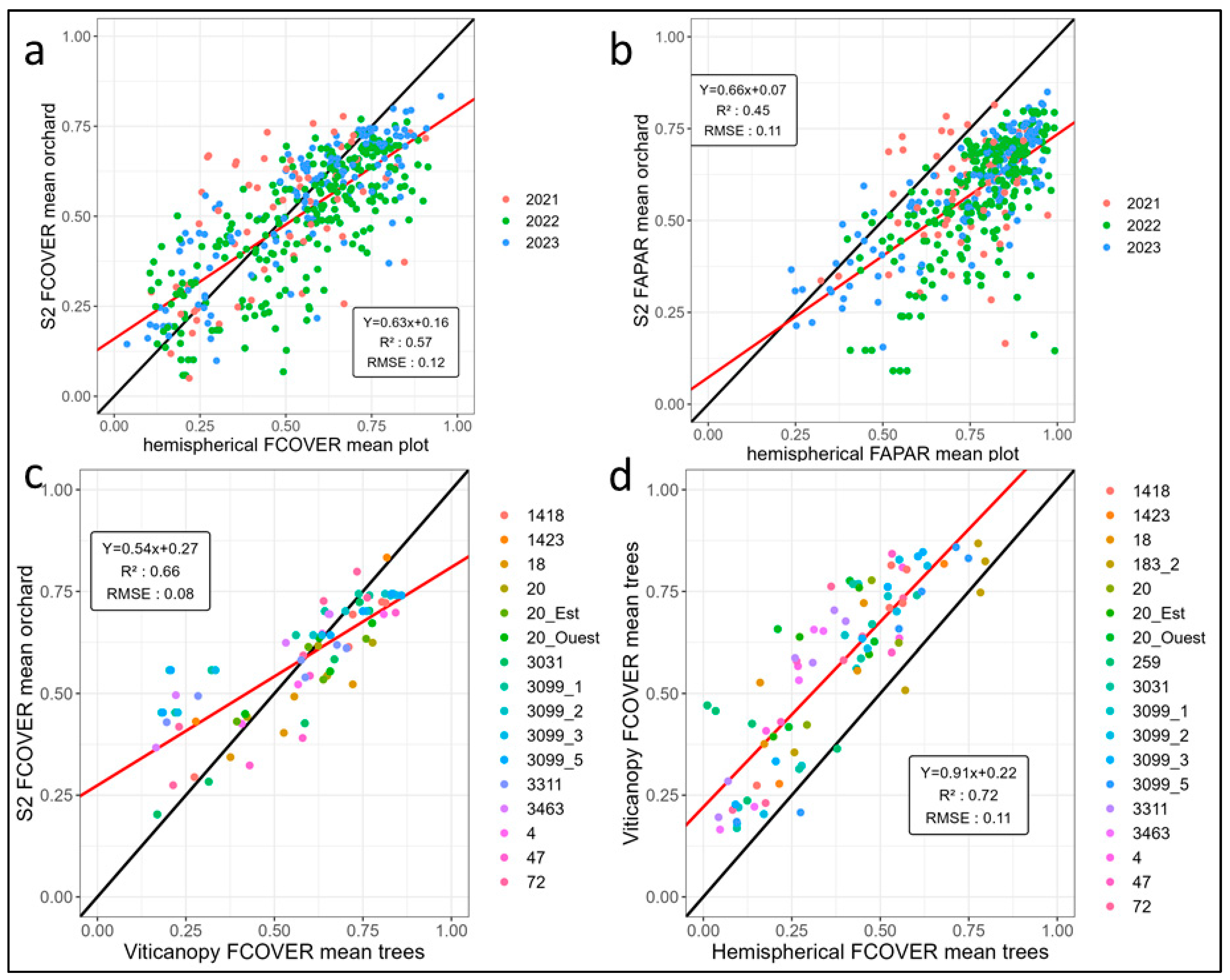
3.1. Analysis of Ground Measurements Compared to Estimations from Sentinel 2

Comparisons between the Sentinel 2 LAI and the PAI results obtained from Viticanopy and ceptometer measurements (protocol P2) are presented in Figure 5 for the first half of 2023 (Results for other plots are presented in Supplementary Figure S5). In all cases, the measurements reflect the same positive trend: an increase from DOY 70 (mid-March) to the beginning of June, corresponding to leaf development, followed by a slight decrease after the fruit harvest (DOY 160) due to decreased irrigation and the subsequent impact on leaves. The ceptometer measurements (blue lines) show a marked spatial variability, which is mainly explained by the heterogeneity of the tree canopy and shadow (two acquisitions were taken 50 cm from the trunk and 20 cm from the middle of the row). While all the trees in a field are pruned at the same period, trees differ in their patterns, growth, crown, and shadow. The farther into the season, the greater the standard deviation. The Viticanopy measurements show less variability due to the smaller view captured by the smartphone. Neither the Viticanopy nor the ceptometer method distinguishes between leaf and non-leaf material. Both methods characterise only the tree canopy, as opposed to Sentinel 2 pixels, which include both the tree canopy and the background due to the inter-row cover. The difference between the Sentinel 2 LAI and the PAI based on these two methods defines the inter-row impact at the pixel scale. For grassed orchards (plot 3099 in the Ouvèze area at left on Figure 5 and plot 4 in La Crau at right), the PAI values from the Viticanopy and ceptometer methods are always lower than the Sentinel 2 LAI values. The inter-row grass in the S2 pixel has a strong impact, particularly at the beginning of the season. After the harvest, when irrigation decreases and the grass becomes yellow, there is less of a difference between the Viticanopy, ceptometer, and Sentinel 2 values. For non-grassed cherry trees with a higher tree density, represented by plot 183 (middle Figure 5b), the PAI from the Viticanopy and ceptometer methods is higher than the LAI from Sentinel 2. The impact of the bare soil results in a lower S2 value.

Scatter plots and correlations between Sentinel 2 LAI data and ceptometer PAI (protocol P2) and Viticanopy PAI measurements across all monitored plots in the two study sites (La Crau and Ouvèze basin) are presented in Figure 6a–c (see additional graphs of comparison with ceptometer protocol 1 in Supplementary Figure S6). The highest correlation for the Sentinel 2 LAI was obtained using the Viticanopy estimates, particularly excluding non-grassed orchards (fields 183.2 and 259, Figure 6c). There is a significant relationship between the ceptometer and Viticanopy values (R² = 0.45 with P1, R² = 0.71 with P2—see Supplementary Figure S6). The ceptometer comparison in Figure 6a shows a lower correlation with the S2 estimation with an R² value at −0.14, mainly due to the large spatial variability of the heterogeneity of the tree canopy and shadows (Figure 6a).

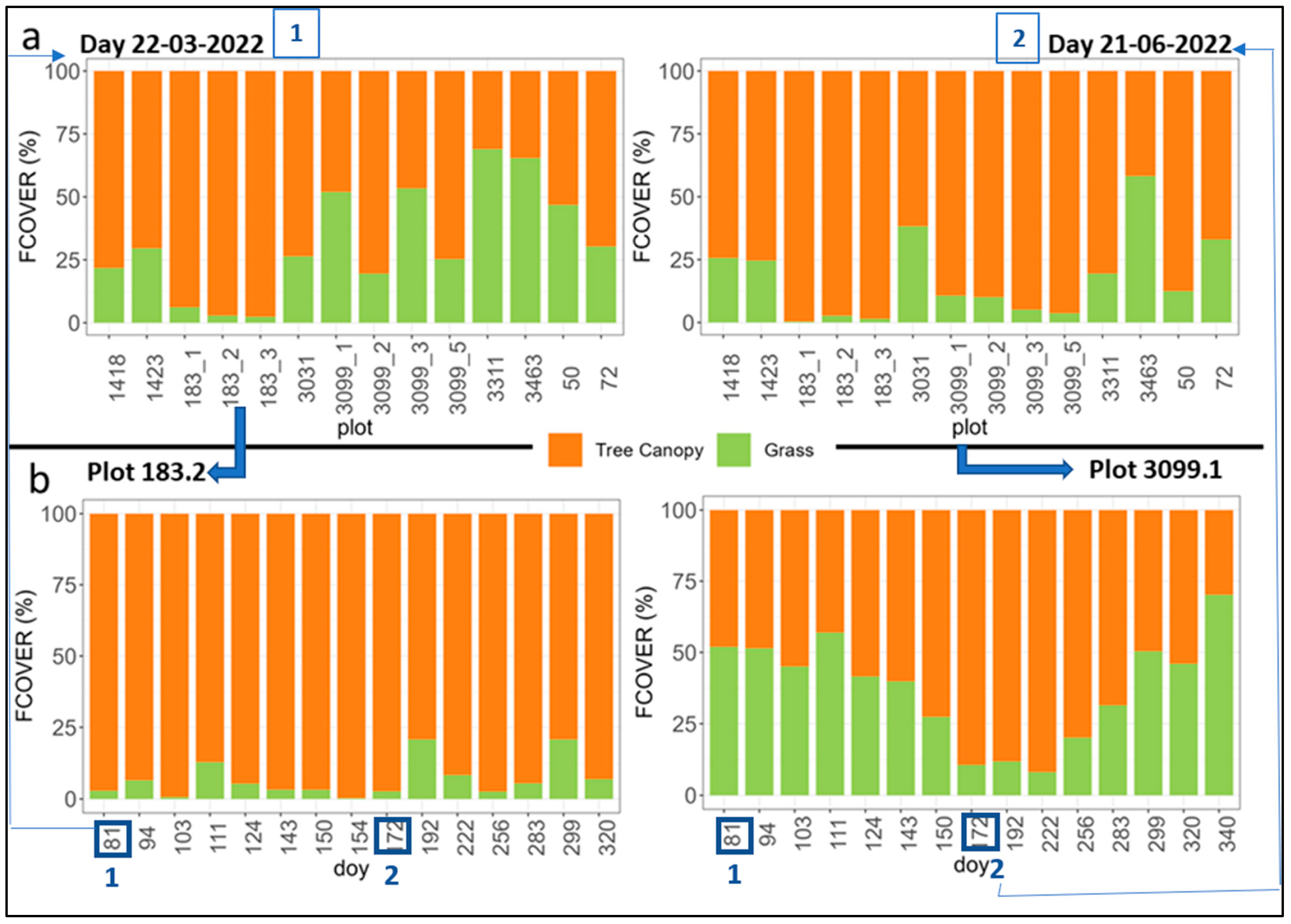
3.2. Analysis of Inter-Row Impact on the Biophysical Variables Assessed from Hemispherical Photographs

The protocols involving hemispherical photographs enable the quantification of the relative impacts of the inter-row and tree canopy at the pixel scale. Figure 7 shows the proportion of the tree (in orange) and inter-row (green) effect calculated from Equation (1) on values obtained from hemispherical photographs taken at cherry orchards in the Ouvèze area. This proportion is computed at a plot scale that is representative of a Sentinel 2 pixel (10 m) for two different days in 2022: 22 March and 21 June in the top graphs (Figure 7a). A significant spatial variability in the grass contribution is observed among the cherry trees, and is more pronounced in March than in June. Such variability can largely be explained by differing agricultural practices: some farms cut the grass or apply weedkiller in the row, which can extend into the inter-row. The plots where the FCOVER or grass remains high tend to correspond to young orchards (e.g., plot 3463). The impact of the tree canopy is greater in June, as leaves and branches are more developed than in March. Some farmers use bands to stretch the branches as far as possible in order to optimise the impact of radiation on the tree, while others cut branches to make it easier for machinery to move about. These different practices induce variations in the structures outlined in these results. The results for the non-grassed field (183) differ substantially from the grassed orchards, showing the FCOVER values close to 100% of the tree canopy proportion, although there is still a small grass fraction due to the grass regrowth between the two treatments. It is important to note that this orchard has the narrowest inter-row spacing as well as a high tree density.

Figure 7b presents the temporal variability for one year (2022) between mid-March and mid-November in the inter-row impact on the FCOVER computed for two different plots (183 non- grassed and 3099 grassed orchards). While a small area of grass can appear on the non-grassed plot due to regrowth, this contribution always remains very low (<5%). For the grassed plot (3099.1, right), the grass contribution varies throughout the year, from 12% in summer to nearly 70% in winter. The variability tends to be correlated with the soil moisture content, especially in spring and in autumn; when there is more rain, the soil water stock is high, and the grass is green and well developed. In summer, soil moisture decreases despite irrigation due to higher evapotranspiration. During these periods, much of the water is preferentially delivered to the trees, and the grass subsequently turns yellow. Thus, the inter-row contribution decreases, and the impact of the tree canopy becomes dominant.

Figure 8a shows the inter-row contribution computed on all the monitored grassed orchards from the hemispherical photographs for 2022 (photographs taken throughout the year outlined in orange). The observed temporal variability is related to differences in grass development and differing farm management practices concerning inter-rows. The contribution of grass is high at the beginning and at the end of the year because the high soil moisture content allows for the maintenance of green cover. To explore the impact of the Sentinel 2 mixed-pixel response, the inter-row contribution (computed in Figure 8a) was subtracted from Sentinel 2-derived biophysical variables. Figure 8b,c show comparisons between the FAPAR (in black) with and without (in green) this inter-row contribution for a non-grassed site (field 183, Figure 8b) and a grassed site (field 1418, Figure 8c).

While there is an obvious and expected grass contribution for field 1418, the impact of the grass signal on the non-grassed site (field 183) is lower, albeit fluctuating slightly during summer due to grass regrowth between the two chemical treatments. The presence of grass has very little impact on the signal of the satellite in this case. In the grassed plot, the signal is highly affected, especially during winter. The grass impact starts to decrease around day 25, with the beginning of tree leaf development in spring and grass-cutting around day 50. Grass development appears to be responsible for the double-curved upward trends observed on the temporal profiles.

3.3. Validation of the Aggregative Model

Figure 9a,b present the correlations between the Sentinel 2 FCOVER (a) and FAPAR (b) computed by the BVNET model and the values obtained from the aggregative model (equation 1 applied with hemispherical photographs) for years 2021 to 2023. Using the aggregative model that considers both trees and inter-rows to compute integrative values for the FCOVER and FAPAR gave satisfactory results, with statistically significant correlation coefficients (R² for FCOVER = 0.57, and R² for FAPAR = 0.45) compared to the Sentinel 2 estimates. There is a slight overestimation of the Sentinel 2 biophysical variables, but this remains acceptable, with an RMSE of 0.12 for the FCOVER and 0.11 for the FAPAR. Thus, the aggregative model can be considered to validate the orchards’ FCOVER and FAPAR estimates provided by Sentinel 2. Figure 9c shows the correlation between the Sentinel 2 FCOVER and Viticanopy FCOVER, which considers only the tree canopy. Figure 9d shows the correlation between the Viticanopy FCOVER and the FCOVER from the upward-aimed hemispherical photographs. Correlation coefficients are slightly higher for the FCOVER than for the FAPAR (Figure 9a,b). The slopes are usually below the 1:1 line, except for the comparison between the Viticanopy and hemispherical FCOVER estimates. The correlation between the FCOVER computed for the tree canopies from hemispherical photographs and using Viticanopy appears quite good, with a high correlation coefficient (0.72) and a low RMSE value (0.11). While an introduced bias is observed, due primarily to the smaller view covered with Viticanopy, this can easily be corrected using these statistical results. In the light of our results, therefore, the Viticanopy approach (Figure 9d) appears to be an easy-to-use tool providing accurate and relevant ground measurements in orchard systems.

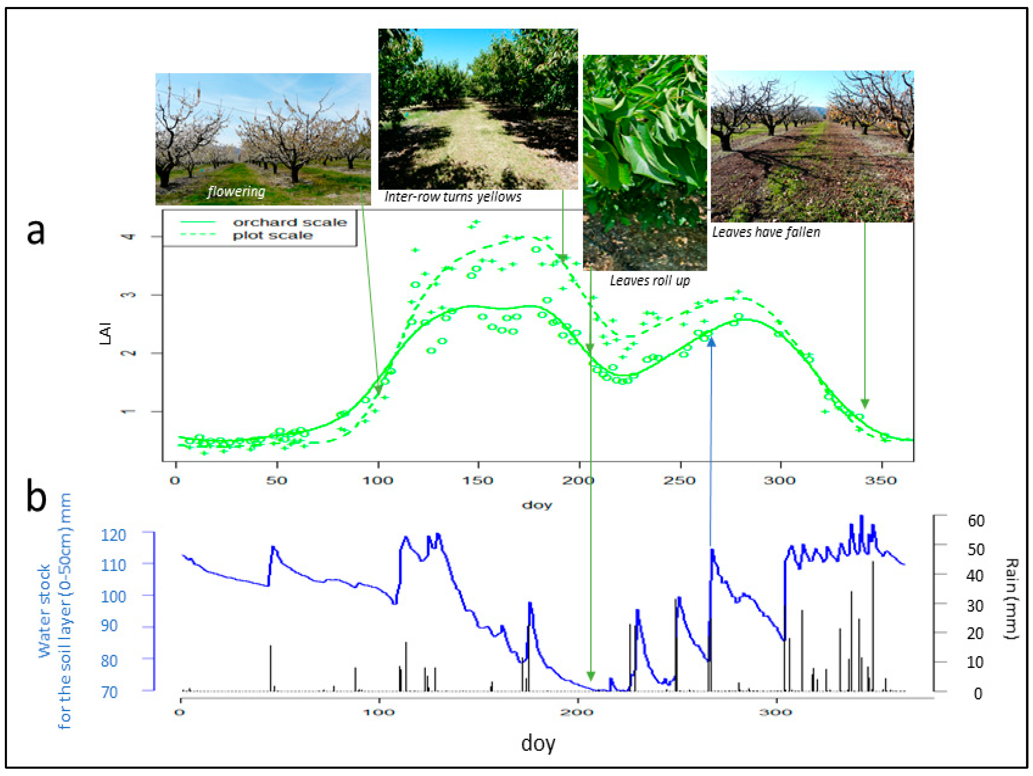
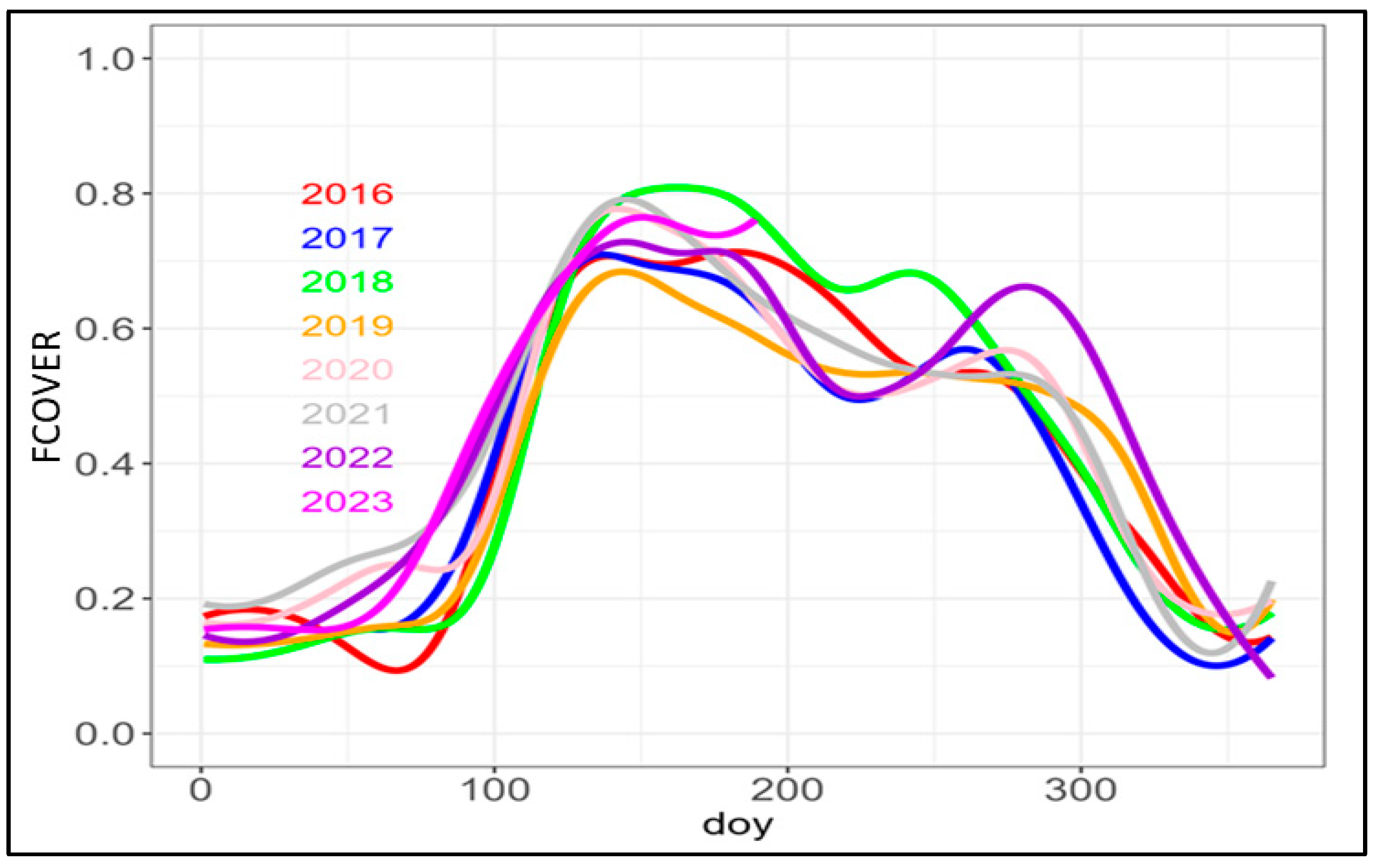
3.4. Analysis of Leaf Development and Identification of Key Phenological Stages from Sentinel 2 Biophysical Variables

Figure 10a shows a temporal profile of the LAI (in green) of grassed cherry trees at two spatial scales, including the plot (dotted lines) and field (solid green line), and Figure 10b shows the soil water stock for the 0–50 cm layer (blue line) for the year 2022.

A rapid increase in the LAI is observed in spring (April to June), when leaves are developing and stems grow, followed by a slight decrease from DOY 180 (July). The LAI decrease can be explained by several factors (hydric stress impacting the leaves, yellowing of the inter-row). After the harvest (generally in June for cherry trees, around DOY 181), irrigation decreases slightly, resulting in less water availability and increasing the risk of leaf “roll up”. In summer, the grass in the inter-row becomes yellow, which impacts the global value recorded at the pixel scale (10 m). In autumn, when rains generally return, the biophysical variables start to increase again, as the inter-row turns green, and tree leaves become less dry. The last stage is reflected in leaves falling and senescence. The evolution of the LAI in this orchard is strongly linked to the soil moisture content, measured here using capacitive sensors and averaged for the 0–50 cm layer. While drip-irrigation is applied from April to September (1 h per day, 6 L/m in spring and 1 h/2–5 days after the harvest), the soil water stock in the 0–50 cm layer decreases from June to September because of the higher evapotranspiration rates, which are also strongly linked to the LAI. At the field scale, a high spatial variability of the LAI is noted due to differing species, with most fields containing at least two different varieties of either early, mid-season, or late varieties (see Figure S2 in Supplementary). Some of the largest fields (e.g., 3099) contain four varieties. Such management practices are reflected in the differences between the averaged value obtained for a field (combining different varieties) and the value extracted at the plot scale (including 3 × 3 trees, LAI Figure 6a, green dotted line). The tree age can also vary at the field scale. When trees suffer too much damage from pests, farmers may cut them down and replant new ones. Soil heterogeneity, particularly in large fields, may also explain the differences observed between the plot and field scale (plots described in Supplementary Figure S2).

This pattern can also vary according to climate conditions in a particular year. Figure 11 shows the temporal profiles of the Sentinel 2 FCOVER from 2016 to 2023 for the same field (3099). The decrease in FCOVER values during the summer period appears more pronounced for drier years (in 2022, annual rainfall of 550 mm; in 2020, 439 mm) than for wetter years, such as 2018 (annual rainfall of 918 mm).

Figure 12a,b present the FAPAR time series in 2022 for two cherry orchards in the Ouvèze area: non-grassed plot 183.1 and grassed plot 3099.1; the vertical lines correspond to the ground observation of the main phenological stages. In these examples, flowering (green vertical line, BBCH 67) occurs at a time when the curve has already started to increase. Similar results obtained in 2021 on several orchards (grassed or non-grassed, with different irrigation practices) are shown in Supplementary Figure S7. As already noted, the flowering date can vary depending on the cultivar (early or late).

Table 3. Dates of fruit set stage (day of year) observed for 2021, 2022, and 2023 on the different cherry trees monitored in the Ouvèze area.

Plot	BBCH 67 2021	BBCH 67 2022	BBCH 67 2023	Plot	BBCH 69 2021	BBCH 69 2022	BBCH 69 2023
50	109 (19/04)	111 (21/04)		50	125 (05/05)	124 (04/05)
72		111 (21/04)	109 (19/04)	72		124 (04/05)	123 (03/05)
183_1		103 (13/04)		183_1		124 (04/05)
183_2		103 (13/04)	104 (14/04)	183_2		124 (04/05)	123 (03/05)
183_3		103 (13/04)		183_3		124 (04/05)
1401	109 (19/04)	111 (21/04)	109 (19/04)	1401	125 (05/05)	124 (04/05)	123 (03/05)
1418	99 (09/04)	94 (04/04)	104 (14/04)	1418	125 (05/05)	111 (21/04)	109 (19/04)
1423		111 (21/04)	109 (19/04)	1423		124 (04/05)	123 (03/05)
1424	99 (09/04)			1424	125 (05/05)
3031		103 (13/04)	104 (14/04)	3031		124 (04/05)	123 (03/05)
3099_1	99 (09/04)	103 (13/04)	104 (14/04)	3099_1	125 (05/05)	124 (04/05)	123 (03/05)
3099_2		111 (21/04)	111 (21/04)	3099_2		124 (04/05)
3099_3		103 (13/04)	111 (21/04)	3099_3		124 (04/05)	123 (03/05)
3099_5		111 (21/04)	111 (21/04)	3099_5		124 (04/05)	123 (03/05)
3311		111 (21/04)	109 (19/04)	3311		124 (04/05)	123 (03/05)
3347	92 (02/04)	103 (13/04)	95 (05/04)	3347	125 (05/05)	111 (21/04)	109 (19/04)
3463		111 (21/04)	109 (19/04)	3463		124 (04/05)	123 (03/05)

shows the dates observed for the monitored fields for the years studied. Field 3099 (Figure 12b) is the largest of the watershed (>4 ha) and contains mainly old trees of several varieties, ranging from very early to late, with grassed inter-rows.

Figure 13 shows the temporal variability observed at this last field (field 3099) across the main phenological stages (BBCH notations). BBCH stage 67 represents the greatest density of open flowers and BBCH stage 69 represents the point at which all the petals fall, which is correlated to the fruit set stage. After this last stage, farmers generally start cherry tree irrigation. As expected, it is mainly from the flowering stage onwards that the dates of this phenological stage vary most. Cherry flowering generally starts in March/April in the south of France [10] and nectarine flowering starts in April/May [99,100]. This key stage for cherry trees is followed by a fruit set stage around 15 days later [101,102], which is characterised by the falling of flower petals. For some stages (between 50 and 57), no variability was observed. However, this lack of variation likely reflects the frequency of observation, which was not dense enough during these periods. A larger number of ground observations were collected closer to the flowering dates (DOY 104–112).

The dates for the phenological stages are slightly later in 2022 and 2023 than in 2021 (see Table 3). In 2021, when fewer plots were monitored, there was already a difference of 17 days in stage 67 observations between fields. In 2023, this shift increased to 28 days. The staggering of the fruit set stage is due to several factors, including climatic conditions, the choice of tree varieties, and the available soil moisture. While stage 67 varied significantly between fields, stage 69 was more stable over time, generally appearing around DOY 123 and 125 each year. As mentioned in Section 2.1.1, most fields contain different varieties to ensure a longer harvesting period. Some fields are also located in a small, colder valley (e.g., field 1401) and receive less radiative input, which may explain why their fruit set stage occurs later than other, more exposed fields located in the plateau (e.g., field 3099). In addition, there were slight variations between the dates of the fruit set stage for 2022 and 2023. Both these years were classified as rather hot and dry in spring compared to 2021, which was wetter. Such climatic variations likely explain the small discrepancies observed between the monitored fields.

Figure 14a shows the normalised FAPAR results expressed in boxplots for the two main stages of interest, based on values extracted for all the orchards in 2021 from Sentinel 2 data. A significant difference between these two stages can be identified from the normalised FAPAR. A normalised FAPAR threshold (FAPAR (n,j > 60%)) distinguishes significantly between the two main phenological stages considered, BBCH 67 and 69. By applying this threshold to the whole normalised FAPAR image on the watershed, it is possible to map the period between the flowering and fruit set stages at the watershed scale. The resulting map is presented in Figure 14b, enabling the orchards already at the fruit set stage to be detected and the appropriate starting point for irrigation on the watershed to be determined.

4. Discussion

4.1. Ground Measurement Protocol to Estimate Biophysical Variables and Comparison with Sentinel 2-Based Estimations

Our study compared different protocols using various ground sensors. Even if the acquisition methods differ, the measurements were performed at the same dates with the same sun and leaf inclinations and on the same trees. To our knowledge, this is the first attempt to use Viticanopy, the ceptometer, and hemispherical photographs for comparison purposes on a variety of orchards. Various studies have shown comparisons between two methods such as [24,46] between ceptometer and PocketLAI methods [61,103] or Viticanopy and LAI 2000 [64,82]. Liu et al. (2013) [104] has discussed the different factors impacting the BVs estimated from different methods. The PAI can replace the tree LAI in certain ranges of the zenith [26,34]. Hemispherical photographs appear to be the best technique, revealing both the inter-row and the tree impacts on biophysical variable values (protocol Supplementary Figure S3), and allowing us to propose an aggregative model to validate the Sentinel 2 estimations (see Figure 9 and Supplementary Figure S4). Inverting the S2 biophysical variables appears achievable using this new approach, with our protocol proposed for validation. The levels of accuracy obtained to validate the BVNET outputs were comparable to those achieved by other studies exploring different crops in various contexts [57,105]. The error on the estimations of the FCOVER and FAPAR remains quite acceptable. The use of the BVNET model for heterogeneous crops is unusual. Other approaches based on geometrical–optical (3D) radiative transfer models (such as DART model https://dart.omp.eu/#/ accessed on 2 August 2024 for example) are well-suited for addressing issues related to shading, background effects, and other complexities inherent in discontinuous canopies such as orchards, but such approaches generally required a lot of input parameters with an accurate description of the tree and leaf, which were not available at our study scale. Our choice to use the BVNET model was motivated by the intention to explore its adaptability and generate comparative observations with a rigorous control with various ground measurements.

The inter-row impact can be quantified at the pixel scale. Numerous photographs allowed the collection of a large dataset for deep-learning image classifications to identify the leaves and grass in the inter-row. A first “expert knowledge” step is required to identify the masks and specify the sky, leaf, grass, or soil. Generally speaking, the larger the learning dataset, the greater the precision. Our ground observations provide a large dataset which can be added to other ground-based data to improve image classification methods for other study cases. It should, however, be mentioned that classifying the soil-facing images is often hindered by heterogeneous surface features (including stones, sparse vegetation, fallen leaves, or grass). Classifying the tree canopy is easier.

Viticanopy or a ceptometer providing PAI values are alternative ways of characterising the tree canopy. For the ceptometer, two protocols derived from López-Lozano and Casterad (2013) [92] were compared (detailed in Figure 3e and comparison of the results in Supplementary Figure S6), neither of which proved particularly satisfactory for orchard applications because of the large spatial variability of orchard structure and the associated shadow. The Viticanopy app showed less variability and was easier to use. Recently, Lai et al. (2022) [106] have proposed a method to correct for the clumping effect by using one-dimensional fractal dimensions. In that study, 3D radiative transfer models were applied to simulate different configurations of crown vegetation canopies. The method warrants further research; the pattern of the orchards studied here could be simulated to evaluate it. Other indirect methods, such the use of LIDAR or UAV [107] have also been proposed, but their applications are spatially limited. Our protocols can be applied in other orchard contexts where ground-based measurements are used to monitor leaf development and evaluate the impact of the inter-row on the validation of BV assessment via Sentinel 2 pixels.

4.2. Sentinel 2 Potential for Orchard Monitoring and the Detection of Key Phenological Stages

This study demonstrated that it is possible to monitor the foliar dynamics of orchards in the Mediterranean region from Sentinel 2 images. Typical dynamic patterns have been observed for orchards, as for many other crop systems, which are strongly related to temporal variations in the soil moisture. The key variables, including the LAI, FCOVER, and FAPAR, can be used to characterise leaf development and we have demonstrated that the normalisation of the FAPAR allowed us to detect some crucial phenology stages (fruit set). The time series from Sentinel 2 for all the monitored biophysical variables show an increase from March to June, then a slight decrease in summer, followed by an increase in autumn. These dynamics stem from different processes related to the water consumption of orchards, depending on both irrigation practices and pedo-climatic conditions [69,108,109]. Notably, it is the first time that the inter-row contribution was quantified at the Sentinel 2 pixel scale, using an original approach based on determining the BVs from hemispherical photographs downward-aimed at the inter-row and upward-aimed at the tree canopy. It is thus possible to quantify the impact of these two factors to determine the relative importance of the grass cover in the spectral signal at the pixel scale. To complete this study, lidar data focused only on the tree canopies could be used to validate the estimations performed at the tree level [104,107]. A different approach developed by Abubakar et al. (2023) [28] was applied to Mediterranean vineyards based on the disaggregation of the Sentinel 2 signal, assuming that in summer the inter-row is bare soil. They employed a phenological model to derive metrics and then subtracted this model from the LAI profile to classify grassed and non-grassed plots. However, this last approach would be difficult to apply in orchards, with their greater diversity of inter-row management and more developed leaf expansion.

We also established that some key phenological stages, including the end of the flowering and fruit set stages, could be identified via a normalised FAPAR through the analysis of nine cherry orchards in the Ouvèze area. This stage is especially important in determining when to start the irrigation of orchards, helping farmers with water management. To detect other phenological stages would require increasing ground observations for validation. As described in particular by Carmona-García et al. (2024) [110], Tubau Comas et al. (2019) [111], or Horton et al. (2017) [112] for other fruit species, the automatic identification of phenological stages by remote sensing is possible, but calibration requires numerous observations on the ground and/or a higher image precision than Sentinel 2 can provide. Other methods based on correlation analysis between various spectral indices derived from Sentinel missions and phenological stages have been explored, but their performance depends on climate years [113,114]. The method based on the use of Sentinel 2 data requires a high frequency of cloud-free images in spring. For tropical countries, where there are more cloudy days, different studies have shown that the ratio between VV and VH from Sentinel 1 radar missions can also be used to fill temporal gaps when monitoring crop development [115]. Other satellites can be used to help with orchard water management, mixing optical and thermal spectral ranges [116,117,118]. The future TRISHNA mission [119], which will be launched in 2026, should also provide high-resolution spatial and temporal thermal data very complementary to Sentinel 2 data.

4.3. Operational Applicability of Methods, Limitations, and Future Research

The LAI, FCOVER, and FAPAR are often used in a range of modelling applications, including simulating soil–vegetation–atmosphere transfers (SVATs) and crop models to predict yields or reproduce water and carbon budgets. However, the assessment of biomass production for orchards is still poorly addressed by functional models. For example, while the generic STICS crop model [120] can simulate a range of crops and technical practices, including vineyards [45,121] and apple trees [122], it is still unable to reproduce cherry tree crops. The introduction into STICS of the LAI derived from Sentinel 2 should help to better simulate the biomass of these fruit trees. This will be one of the avenues to explore in the future, through similar approaches developed by Courault et al. (2021, 2010) [17,123]. Water needs can be estimated using various models, some simplified via the use of crop coefficients defined according to the FAO56 method [19]. In the same way, this method can be improved by computing crop coefficients from the Sentinel 2 FCOVER [108]. Moreover, being able to distinguish the relative impacts of grass and tree canopy at the plot scale provides more useful information on water consumption.

While several applications suggest themselves from these first results, it remains important to evaluate our methods in different environmental contexts. The impact of phytosanitary treatments and fertilisers has not been mentioned here. Contamination by pests or the provision of inputs can modify trees’ foliar dynamics [124], as can the development and composition of the grass cover [125,126]. Monitoring such impacts requires detailed knowledge of agricultural practices and specific ground observations. Some studies have explored these factors using a spectroradiometer or UAV sensors [14,127]. This is a research avenue of its own to be explored in the remote sensing field over the coming years and should enhance orchard management.

5. Conclusions

Here, we have established that Sentinel 2 data can be used to monitor orchard development in Mediterranean regions. For the first time, three different ground-based methods were compared to validate BV values estimated from satellite images via the BVNET model. The validation of the Sentinel 2 LAI was performed using Viticanopy, which proved to be easy to use for monitoring leaf development, providing reliable results. We propose a new aggregative model applied to values derived from hemispherical photographs; combining inter-row and tree impacts, the model can be used to quantify the proportions of the signal linked to grass cover and to trees. This original approach provides a better understanding of the inverting of biophysical variables from Sentinel 2. Our results show statistically significant correlation coefficients for the Sentinel 2-based FCOVER and FAPAR compared to values obtained from the aggregative model. Very few studies have explored a range of different methods on commercial orchards combining, for example, late- and early-fruiting varieties of cherry trees, apricots, and nectarines. Importantly, all the proposed methods can be applied in other orchard contexts. This study also demonstrated that some key phenological stages of cherry trees, like the end of the flowering and fruit set stages, which determine the start of irrigation in our studied regions, can be identified via the normalisation of the FAPAR. The enhanced characterisation of plant phenological development from space offers a range of opportunities for improved orchard management, particularly concerning the efficient use of irrigation scheduling and yield prediction.

References

1. Cherif, S.; Doblas-Miranda, E.; Lionello, P.; Borrego, C.; Giorgi, F.; Rilov, G.; Iglesias, A.; Jebari, S.; Mahmoudi, E.; Moriondo, M.; et al. Drivers of Change. In Climate and Environmental Change in the Mediterranean Basin–Current Situation and Risks for the Future; First Mediterranean Assessment Report; Union for the Mediterranean, Plan Bleu, UNEP/MAP: Marseille, France, 2020; pp. 59–180. [Google Scholar] [CrossRef]
2. MedECC. Climate and Environmental Change in the Mediterranean Basin–Current Situation and Risks for the Future; First Mediterranean Assessment Report; Union for the Mediterranean, Plan Bleu, UNEP/MAP: Marseille, France, 2020; ISBN 978-2-9577416-0-1. [Google Scholar] [CrossRef]
3. Nagai, S.; Saitoh, T.M.; Yoshitake, S. Cultural Ecosystem Services Provided by Flowering of Cherry Trees under Climate Change: A Case Study of the Relationship between the Periods of Flowering and Festivals. Int. J. Biometeorol. 2019, 63, 1051–1058. [Google Scholar] [CrossRef] [PubMed]
4. Benmoussa, H.; Ben Mimoun, M.; Ghrab, M.; Luedeling, E. Climate Change Threatens Central Tunisian Nut Orchards. Int. J. Biometeorol. 2018, 62, 2245–2255. [Google Scholar] [CrossRef] [PubMed]
5. Campoy, J.A.; Ruiz, D.; Egea, J. Dormancy in Temperate Fruit Trees in a Global Warming Context: A Review. Sci. Hortic. 2011, 130, 357–372. [Google Scholar] [CrossRef]
6. El Yaacoubi, A.; Malagi, G.; Oukabli, A.; Hafidi, M.; Legave, J.-M. Global Warming Impact on Floral Phenology of Fruit Trees Species in Mediterranean Region. Sci. Hortic. 2014, 180, 243–253. [Google Scholar] [CrossRef]
7. Primack, R.B.; Higuchi, H.; Miller-Rushing, A.J. The Impact of Climate Change on Cherry Trees and Other Species in Japan. Biol. Conserv. 2009, 142, 1943–1949. [Google Scholar] [CrossRef]
8. Mihailescu, E.; Bruno Soares, M. The Influence of Climate on Agricultural Decisions for Three European Crops: A Systematic Review. Front. Sustain. Food Syst. 2020, 4, 64. [Google Scholar] [CrossRef]
9. Fernández, J.E. Plant-Based Sensing to Monitor Water Stress: Applicability to Commercial Orchards. Agric. Water Manag. 2014, 142, 99–109. [Google Scholar] [CrossRef]
10. Bujdosó, G.; Hrotko, K. Cherry Production. In Cherries: Botany, Production and Uses; CABI: Wallingford, UK, 2017; pp. 1–13. ISBN 978-1-78064-837-8. [Google Scholar]
11. Blanco, V.; Blaya-Ros, P.J.; Castillo, C.; Soto-Vallés, F.; Torres-Sánchez, R.; Domingo, R. Potential of UAS-Based Remote Sensing for Estimating Tree Water Status and Yield in Sweet Cherry Trees. Remote Sens. 2020, 12, 2359. [Google Scholar] [CrossRef]
12. Fadón, E.; Herrero, M.; Rodrigo, J. Flower Development in Sweet Cherry Framed in the BBCH Scale. Sci. Hortic. 2015, 192, 141–147. [Google Scholar] [CrossRef]
13. Gobin, A.; Sallah, A.-H.M.; Curnel, Y.; Delvoye, C.; Weiss, M.; Wellens, J.; Piccard, I.; Planchon, V.; Tychon, B.; Goffart, J.-P.; et al. Crop Phenology Modelling Using Proximal and Satellite Sensor Data. Remote Sens. 2023, 15, 2090. [Google Scholar] [CrossRef]
14. Guimarães, N.; Sousa, J.J.; Pádua, L.; Bento, A.; Couto, P. Remote Sensing Applications in Almond Orchards: A Comprehensive Systematic Review of Current Insights, Research Gaps, and Future Prospects. Appl. Sci. 2024, 14, 1749. [Google Scholar] [CrossRef]
15. Shin, N.; Saitoh, T.M.; Takeuchi, Y.; Miura, T.; Aiba, M.; Kurokawa, H.; Onoda, Y.; Ichii, K.; Nasahara, K.N.; Suzuki, R.; et al. Review: Monitoring of Land Cover Changes and Plant Phenology by Remote-Sensing in East Asia. Ecol. Res. 2023, 38, 111–133. [Google Scholar] [CrossRef]
16. Wu, B.; Zhang, M.; Zeng, H.; Tian, F.; Potgieter, A.B.; Qin, X.; Yan, N.; Chang, S.; Zhao, Y.; Dong, Q.; et al. Challenges and Opportunities in Remote Sensing-Based Crop Monitoring: A Review. Natl. Sci. Rev. 2023, 10, nwac290. [Google Scholar] [CrossRef]
17. Courault, D.; Hossard, L.; Demarez, V.; Dechatre, H.; Irfan, K.; Baghdadi, N.; Flamain, F.; Ruget, F. STICS Crop Model and Sentinel-2 Images for Monitoring Rice Growth and Yield in the Camargue Region. Agron. Sustain. Dev. 2021, 41, 49. [Google Scholar] [CrossRef]
18. Rivas, H.; Delbart, N.; Ottlé, C.; Maignan, F.; Vaudour, E. Disaggregated PROBA-V Data Allows Monitoring Individual Crop Phenology at a Higher Observation Frequency than Sentinel-2. Int. J. Appl. Earth Obs. Geoinf. 2021, 104, 102569. [Google Scholar] [CrossRef]
19. Sun, X.; Zhou, Y.; Jia, S.; Shao, H.; Liu, M.; Tao, S.; Dai, X. Impacts of Mining on Vegetation Phenology and Sensitivity Assessment of Spectral Vegetation Indices to Mining Activities in Arid/Semi-Arid Areas. J. Environ. Manag. 2024, 356, 120678. [Google Scholar] [CrossRef]
20. Boschetti, M.; Stroppiana, D.; Brivio, P.A.; Bocchi, S. Multi-Year Monitoring of Rice Crop Phenology through Time Series Analysis of MODIS Images. Int. J. Remote Sens. 2009, 30, 4643–4662. [Google Scholar] [CrossRef]
21. Duchemin, B.; Hadria, R.; Er-Raki, S.; Boulet, G.; Maisongrande, P.; Chehbouni, A.; Escadafal, R.; Ezzahar, J.; Hoedjes, J.; Kharrou, H.; et al. Monitoring Wheat Phenology and Irrigation in Central Morocco: On the Use of Relationships between Evapotranspiration, Crops Coefficients, Leaf Area Index and Remotely-Sensed Vegetation Indices. Agric. Water Manag. 2006, 97, 1–27. [Google Scholar] [CrossRef]
22. Nasrallah, A.; Baghdadi, N.; El Hajj, M.; Darwish, T.; Belhouchette, H.; Faour, G.; Darwich, S.; Mhawej, M. Sentinel-1 Data for Winter Wheat Phenology Monitoring and Mapping. Remote Sens. 2019, 11, 2228. [Google Scholar] [CrossRef]
23. Kowalski, K.; Senf, C.; Hostert, P.; Pflugmacher, D. Characterizing Spring Phenology of Temperate Broadleaf Forests Using Landsat and Sentinel-2 Time Series. Int. J. Appl. Earth Obs. Geoinf. 2020, 92, 102172. [Google Scholar] [CrossRef]
24. Quesada-Ruiz, L.C.; Caparros-Santiago, J.A.; Garcia-Perez, M.A.; Rodriguez-Galiano, V. Characterising the Spring and Autumn Land Surface Phenology of Macaronesian Species Using Sentinel-2 Data: The Case of Canary Island. In Proceedings of the Remote Sensing for Agriculture, Ecosystems, and Hydrology XXIII, Online, 13–17 September 2021; Neale, C.M., Maltese, A., Eds.; SPIE: Bellingham, WA, USA, 2021; p. 7. [Google Scholar]
25. Grabska-Szwagrzyk, E.; Tymińska-Czabańska, L. Sentinel-2 Time Series: A Promising Tool in Monitoring Temperate Species Spring Phenology. For. Int. J. For. Res. 2024, 97, 267–281. [Google Scholar] [CrossRef]
26. Misra, G.; Cawkwell, F.; Wingler, A. Status of Phenological Research Using Sentinel-2 Data: A Review. Remote Sens. 2020, 12, 2760. [Google Scholar] [CrossRef]
27. Sawant, S.A.; Chakraborty, M.; Suradhaniwar, S.; Adinarayana, J.; Durbha, S.S. Time Series Analysis of Remote Sensing Observations for Citrus Crop Growth Stage and Evapotranspiration Estimation. Int. Arch. Photogramm. Remote Sens. Spat. Inf. Sci. 2016, XLI-B8, 1037–1042. [Google Scholar] [CrossRef]
28. Abubakar, M.A.; Chanzy, A.; Flamain, F.; Courault, D. Characterisation of Grapevine Canopy Leaf Area and Inter-Row Management Using Sentinel-2 Time Series. OENO One 2023, 57. [Google Scholar] [CrossRef]
29. Rao, P.; Zhou, W.; Bhattarai, N.; Srivastava, A.K.; Singh, B.; Poonia, S.; Lobell, D.B.; Jain, M. Using Sentinel-1, Sentinel-2, and Planet Imagery to Map Crop Type of Smallholder Farms. Remote Sens. 2021, 13, 1870. [Google Scholar] [CrossRef]
30. Zarco-Tejada, P.J.; Hornero, A.; Beck, P.S.A.; Kattenborn, T.; Kempeneers, P.; Hernández-Clemente, R. Chlorophyll Content Estimation in an Open-Canopy Conifer Forest with Sentinel-2A and Hyperspectral Imagery in the Context of Forest Decline. Remote Sens. Environ. 2019, 223, 320–335. [Google Scholar] [CrossRef]
31. Fang, H.; Baret, F.; Plummer, S.; Schaepman-Strub, G. An Overview of Global Leaf Area Index (LAI): Methods, Products, Validation, and Applications. Rev. Geophys. 2019, 57, 739–799. [Google Scholar] [CrossRef]
32. Monteith, J.L. Principles of Environmental Physics. Agric. Meteorol. 1973, 13, 429–430. [Google Scholar] [CrossRef]
33. Weiss, M.; Jacob, F.; Duveiller, G. Remote Sensing for Agricultural Applications: A Meta-Review. Remote Sens. Environ. 2020, 236, 111402. [Google Scholar] [CrossRef]
34. Weiss, M.; Baret, F.; Jay, S. S2ToolBox Level 2 Products LAI, FAPAR, FCOVER 2.0. 2020. Available online: https://step.esa.int/docs/extra/ATBD_S2ToolBox_V2.1.pdf (accessed on 2 August 2024).
35. López-Lozano, R.; Baret, F.; García de Cortázar-Atauri, I.; Bertrand, N.; Casterad, M.A. Optimal Geometric Configuration and Algorithms for LAI Indirect Estimates under Row Canopies: The Case of Vineyards. Agric. For. Meteorol. 2009, 149, 1307–1316. [Google Scholar] [CrossRef]
36. Gower, S.T.; Kucharik, C.J.; Norman, J.M. Direct and Indirect Estimation of Leaf Area Index, fAPAR, and Net Primary Production of Terrestrial Ecosystems. Remote Sens. Environ. 1999, 70, 29–51. [Google Scholar] [CrossRef]
37. Prince, S.D. Satellite Remote Sensing of Primary Production: Comparison of Results for Sahelian Grasslands 1981–1988. Int. J. Remote Sens. 1991, 12, 1301–1311. [Google Scholar] [CrossRef]
38. Shobairi, S.R.; Roudbari, S.H.; Ayombekov, Q.; Sadeghi, H.; Beirami, B.; Pirbasti, M. Tracking the Impact of Climate Factors on Vegetation Dynamics across the Alashan Plateau Semi Desert Ecoregion. Comput. Ecol. Softw. 2024, 14, 77. [Google Scholar]
39. Belda, S.; Pipia, L.; Verrelst, J. Trends in Satellite Time Series Processing for Vegetation Phenology Monitoring. In Multitemporal Earth Observation Image Analysis; John Wiley & Sons, Ltd.: Hoboken, NJ, USA, 2024; pp. 151–183. ISBN 978-1-394-30665-7. [Google Scholar]
40. Han, D.; Cai, H.; Zhang, L.; Wen, Y. Multi-Sensor High Spatial Resolution Leaf Area Index Estimation by Combining Surface Reflectance with Vegetation Indices for Highly Heterogeneous Regions: A Case Study of the Chishui River Basin in Southwest China. Ecol. Inform. 2024, 80, 102489. [Google Scholar] [CrossRef]
41. Camacho, F.; Martínez-Sánchez, E.; Brown, L.A.; Morris, H.; Morrone, R.; Williams, O.; Dash, J.; Origo, N.; Sánchez-Zapero, J.; Boccia, V. Validation and Conformity Testing of Sentinel-3 Green Instantaneous FAPAR and Canopy Chlorophyll Content Products. Remote Sens. 2024, 16, 2698. [Google Scholar] [CrossRef]
42. López-Lozano, R.; Duveiller, G.; Seguini, L.; Meroni, M.; García-Condado, S.; Hooker, J.; Leo, O.; Baruth, B. Towards Regional Grain Yield Forecasting with 1km-Resolution EO Biophysical Products: Strengths and Limitations at Pan-European Level. Agric. For. Meteorol. 2015, 206, 12–32. [Google Scholar] [CrossRef]
43. Ines, A.V.M.; Das, N.N.; Hansen, J.W.; Njoku, E.G. Assimilation of Remotely Sensed Soil Moisture and Vegetation with a Crop Simulation Model for Maize Yield Prediction. Remote Sens. Environ. 2013, 138, 149–164. [Google Scholar] [CrossRef]
44. Li, L.; Mu, X.; Jiang, H.; Chianucci, F.; Hu, R.; Song, W.; Qi, J.; Liu, S.; Zhou, J.; Chen, L.; et al. Review of Ground and Aerial Methods for Vegetation Cover Fraction (fCover) and Related Quantities Estimation: Definitions, Advances, Challenges, and Future Perspectives. ISPRS J. Photogramm. Remote Sens. 2023, 199, 133–156. [Google Scholar] [CrossRef]
45. Valdés-Gómez, H.; Celette, F.; de Cortázar-Atauri, I.G.; Jara-Rojas, F.; Ortega-Farías, S.; Gary, C. Modelling Soil Water Content and Grapevine Growth and Development with the Stics Crop-Soil Model under Two Different Water Management Strategies. OENO One 2009, 43, 13–28. [Google Scholar] [CrossRef]
46. Weiss, M.; Baret, F.; Leroy, M.; Hautecoeur, O.; Bacour, C.; Prévot, L.; Bruguier, N. Validation d’une Méthode Basée Sur l’utilisation de Réseaux de Neurones Pour l’estimation de Variables Biophysiques Des Couverts Végétaux à Partir de Données de Télédétection. Agronomie 2002, 22, 547–553. [Google Scholar] [CrossRef]
47. Kalaitzidis, C.; Heinzel, V.; Zianis, D. A Review of Multispectral Vegetation Indices for Biomass Estimation. In Imagin[e,g] Europe; IOS Press: Amsterdam, The Netherlands, 2010; pp. 201–208. [Google Scholar] [CrossRef]
48. Odi-Lara, M.; Campos, I.; Neale, C.M.U.; Ortega-Farías, S.; Poblete-Echeverría, C.; Balbontín, C.; Calera, A. Estimating Evapotranspiration of an Apple Orchard Using a Remote Sensing-Based Soil Water Balance. Remote Sens. 2016, 8, 253. [Google Scholar] [CrossRef]
49. Pôças, I.; Paço, T.A.; Paredes, P.; Cunha, M.; Pereira, L.S. Estimation of Actual Crop Coefficients Using Remotely Sensed Vegetation Indices and Soil Water Balance Modelled Data. Remote Sens. 2015, 7, 2373–2400. [Google Scholar] [CrossRef]
50. Dong, X.; Zhang, Z.; Yu, R.; Tian, Q.; Zhu, X. Extraction of Information about Individual Trees from High-Spatial-Resolution UAV-Acquired Images of an Orchard. Remote Sens. 2020, 12, 133. [Google Scholar] [CrossRef]
51. Özdarici-OK, A.; Ok, A. Using Remote Sensing to Identify Individual Tree Species in Orchards: A Review. Sci. Hortic. 2023, 321, 112333. [Google Scholar] [CrossRef]
52. Park, S.; Nolan, A.; Ryu, D.; Fuentes, S.; Hernandez, E.; Chung, H.; O’Connell, M. Estimation of Crop Water Stress in a Nectarine Orchard Using High-Resolution Imagery from Unmanned Aerial Vehicle (UAV). In Proceedings of the 21st International Congress on Modelling and Simulation, Gold Coast, QLD, Australia, 29 November–4 December 2015; Volume 29. [Google Scholar]
53. Houborg, R.; McCabe, M. Application of a Regularized Model Inversion System (REGFLEC) to Multi-Temporal RapidEye Imagery for Retrieving Vegetation Characteristics. In Proceedings of the SPIE Remote Sensing Conference, Toulouse, France, 21–24 September 2015. [Google Scholar]
54. Bréda, N.J.J. Ground-based Measurements of Leaf Area Index: A Review of Methods, Instruments and Current Controversies. J. Exp. Bot. 2003, 54, 2403–2417. [Google Scholar] [CrossRef]
55. Jonckheere, I.; Fleck, S.; Nackaerts, K.; Muys, B.; Coppin, P.; Weiss, M.; Baret, F. Review of Methods for in Situ Leaf Area Index Determination: Part I. Theories, Sensors and Hemispherical Photography. Agric. For. Meteorol. 2004, 121, 19–35. [Google Scholar] [CrossRef]
56. Weiss, M.; Baret, F.; Smith, G.J.; Jonckheere, I.; Coppin, P. Review of Methods for in Situ Leaf Area Index (LAI) Determination: Part II. Estimation of LAI, Errors and Sampling. Agric. For. Meteorol. 2004, 121, 37–53. [Google Scholar] [CrossRef]
57. Demarez, V.; Duthoit, S.; Baret, F.; Weiss, M.; Dedieu, G. Estimation of Leaf Area and Clumping Indexes of Crops with Hemispherical Photographs. Agric. For. Meteorol. 2008, 148, 644–655. [Google Scholar] [CrossRef]
58. Andrieu, B.; Allirand, J.M.; Jaggard, K. Ground Cover and Leaf Area Index of Maize and Sugar Beet Crops. Agronomie 1997, 17, 315–321. [Google Scholar] [CrossRef]
59. Jackson, J.E. The Biology of Apples and Pears; Cambridge University Press: New York, NY, USA, 2003; ISBN 978-1-139-43705-9. [Google Scholar]
60. Steiner, M.; Magyar, L.; Gueviki, M.; Hrotkó, K. Optimization of Light Interception in Intensive Sweet Cherry Orchard. Horticulture 2015, LIX. Available online: https://horticulturejournal.usamv.ro/pdf/2015/art17.pdf (accessed on 2 August 2024).
61. Pokovai, K.; Fodor, N. Adjusting Ceptometer Data to Improve Leaf Area Index Measurements. Agronomy 2019, 9, 866. [Google Scholar] [CrossRef]
62. Rich, P.M. Characterizing Plant Canopies with Hemispherical Photographs. Remote Sens. Rev. 1990, 5, 13–29. [Google Scholar] [CrossRef]
63. Weiss, M.; Baret, F.; de Solan, B.; Demarez, V. CAN-EYE, logiciel de traitement d’images pour l’estimation de l’indice foliaire. Cah. Tech. L’inra 2008, 159. Available online: https://hal.science/hal-01496819/document (accessed on 2 August 2024).
64. De Bei, R.; Fuentes, S.; Gilliham, M.; Tyerman, S.; Edwards, E.; Bianchini, N.; Smith, J.; Collins, C. VitiCanopy: A Free Computer App to Estimate Canopy Vigor and Porosity for Grapevine. Sensors 2016, 16, 585. [Google Scholar] [CrossRef] [PubMed]
65. Makhloufi, A.; Kallel, A.; Chaker, R.; Gastellu-Etchegorry, J.-P. Retrieval of Olive Tree Biophysical Properties from Sentinel-2 Time Series Based on Physical Modelling and Machine Learning Technique. Int. J. Remote Sens. 2021, 42, 8542–8571. [Google Scholar] [CrossRef]
66. Orlando, F.; Movedi, E.; Paleari, L.; Gilardelli, C.; Foi, M.; Dell’Oro, M.; Confalonieri, R. Estimating Leaf Area Index in Tree Species Using the PocketLAI Smart App. Appl. Veg. Sci. 2015, 18, 716–723. [Google Scholar] [CrossRef]
67. Poblete-Echeverría, C.; Fuentes, S.; Ortega-Farias, S.; Gonzalez-Talice, J.; Yuri, J.A. Digital Cover Photography for Estimating Leaf Area Index (LAI) in Apple Trees Using a Variable Light Extinction Coefficient. Sensors 2015, 15, 2860–2872. [Google Scholar] [CrossRef]
68. Majasalmi, T.; Rautiainen, M.; Stenberg, P.; Lukeš, P. An Assessment of Ground Reference Methods for Estimating LAI of Boreal Forests. For. Ecol. Manag. 2013, 292, 10–18. [Google Scholar] [CrossRef]
69. Rouault, P.; Courault, D.; Flamain, F.; Pouget, G.; Doussan, C.; Lopez-Lozano, R.; McCabe, M.; Debolini, M. High-Resolution Satellite Imagery to Assess Orchard Characteristics Impacting Water Use. Agric. Water Manag. 2024, 295, 108763. [Google Scholar] [CrossRef]
70. Paltineanu, C.; Chitu, E. Climate Change Impact on Phenological Stages of Sweet and Sour Cherry Trees in a Continental Climate Environment. Sci. Hortic. 2020, 261, 109011. [Google Scholar] [CrossRef]
71. Vilà, M.; Sardans, J. Plant Competition in Mediterranean-type Vegetation. J. Veg. Sci. 1999, 10, 281–294. [Google Scholar] [CrossRef]
72. Abubakar, M.A.; Chanzy, A.; Flamain, F.; Pouget, G.; Courault, D. Delineation of Orchard, Vineyard, and Olive Trees Based on Phenology Metrics Derived from Time Series of Sentinel-2. Remote Sens. 2023, 15, 2420. [Google Scholar] [CrossRef]
73. Mohammed, G. Modélisation Biogéochimique du Système “Irrigation-Sol-Plante-Nappe”: Application à la Durabilité du Système de Culture du foin de Crau. Doctoral Thesis, Université d’Avignon, Avignon, France, 2017; p. 285. [Google Scholar]
74. Trolard, F.; Bourrié, G.; Baillieux, A.; Buis, S.; Chanzy, A.; Clastre, P.; Closet, J.-F.; Courault, D.; Dangeard, M.-L.; Di Virgilio, N.; et al. The PRECOS Framework: Measuring the Impacts of the Global Changes on Soils, Water, Agriculture on Territories to Better Anticipate the Future. J. Environ. Manag. 2016, 181, 590–601. [Google Scholar] [CrossRef] [PubMed]
75. Olioso, A.; Lecerf, R.; Baillieux, A.; Chanzy, A.; Ruget, F.; Banton, O.; Lecharpentier, P.; Trolard, F.; Cognard-Plancq, A.-L. Modelling of Drainage and Hay Production over the Crau Aquifer for Analysing Impact of Global Change on Aquifer Recharge. Procedia Environ. Sci. 2013, 19, 691–700. [Google Scholar] [CrossRef]
76. Djamai, N.; Fernandes, R.; Weiss, M.; McNairn, H.; Goïta, K. Validation of the Sentinel Simplified Level 2 Product Prototype Processor (SL2P) for Mapping Cropland Biophysical Variables Using Sentinel-2/MSI and Landsat-8/OLI Data. Remote Sens. Environ. 2019, 225, 416–430. [Google Scholar] [CrossRef]
77. Weiss, M.; Baret, F. Evaluation of Canopy Biophysical Variable Retrieval Performances from the Accumulation of Large Swath Satellite Data. Remote Sens. Environ. 1999, 70, 293–306. [Google Scholar] [CrossRef]
78. Claverie, M.; Vermote, E.F.; Weiss, M.; Baret, F.; Hagolle, O.; Demarez, V. Validation of Coarse Spatial Resolution LAI and FAPAR Time Series over Cropland in Southwest France. Remote Sens. Environ. 2013, 139, 216–230. [Google Scholar] [CrossRef]
79. Delloye, C.; Weiss, M.; Defourny, P. Retrieval of the Canopy Chlorophyll Content from Sentinel-2 Spectral Bands to Estimate Nitrogen Uptake in Intensive Winter Wheat Cropping Systems. Remote Sens. Environ. 2018, 216, 245–261. [Google Scholar] [CrossRef]
80. Zérah, Y.; Valero, S.; Inglada, J. Physics-constrained deep learning for biophysical parameter retrieval from Sentinel-2 images: Inversion of the PROSAIL model. Remote Sens. Environ. 2024, 312, 114309. [Google Scholar] [CrossRef]
81. Eilers, P.H.C. A Perfect Smoother. Anal. Chem. 2003, 75, 3631–3636. [Google Scholar] [CrossRef]
82. Pichon, L.; Taylor, J.; Tisseyre, B. Using Smartphone Leaf Area Index Data Acquired in a Collaborative Context within Vineyards in Southern France. OENO One 2020, 54, 123–130. [Google Scholar] [CrossRef]
83. Xue, J.; Fan, Y.; Su, B.; Fuentes, S. Assessment of Canopy Vigor Information from Kiwifruit Plants Based on a Digital Surface Model from Unmanned Aerial Vehicle Imagery. Int. J. Agric. Biol. Eng. 2019, 12, 165–171. [Google Scholar] [CrossRef]
84. Fuentes, S.; Chacon, G.; Torrico, D.D.; Zarate, A.; Gonzalez Viejo, C. Spatial Variability of Aroma Profiles of Cocoa Trees Obtained through Computer Vision and Machine Learning Modelling: A Cover Photography and High Spatial Remote Sensing Application. Sensors 2019, 19, 3054. [Google Scholar] [CrossRef] [PubMed]
85. Tongson, E.J.; Fuentes, S.; Carrasco-Benavides, M.; Mora, M. Canopy Architecture Assessment of Cherry Trees by Cover Photography Based on Variable Light Extinction Coefficient Modelled Using Artificial Neural Networks. Acta Hortic. 2019, 1235, 183–188. [Google Scholar] [CrossRef]
86. Ilniyaz, O.; Kurban, A.; Du, Q. Leaf Area Index Estimation of Pergola-Trained Vineyards in Arid Regions Based on UAV RGB and Multispectral Data Using Machine Learning Methods. Remote Sens. 2022, 14, 415. [Google Scholar] [CrossRef]
87. Champion, G.T.; Froud-Williams, R.J.; Holland, J.M. Interactions between Wheat (Triticum aestivum L.) Cultivar, Row Spacing and Density and the Effect on Weed Suppression and Crop Yield. Ann. Appl. Biol. 1998, 133, 443–453. [Google Scholar] [CrossRef]
88. Francone, C.; Pagani, V.; Foi, M.; Cappelli, G.; Confalonieri, R. Comparison of Leaf Area Index Estimates by Ceptometer and PocketLAI Smart App in Canopies with Different Structures. Field Crops Res. 2014, 155, 38–41. [Google Scholar] [CrossRef]
89. Keane, R.E.; Reinhardt, E.D.; Scott, J.; Gray, K.; Reardon, J. Estimating Forest Canopy Bulk Density Using Six Indirect Methods. Can. J. For. Res. 2005, 35, 724–739. [Google Scholar] [CrossRef]
90. Lopes, D.; Nunes, L.; Walford, N.; Aranha, J.; Sette, C.J.; Viana, H.; Hernandez, C. A Simplified Methodology for the Correction of Leaf Area Index (LAI) Measurements Obtained by Ceptometer with Reference to Pinus Portuguese Forests. iFor.-Biogeosci. For. 2014, 7, 186. [Google Scholar] [CrossRef]
91. Wünsche, J.N.; Lakso, A.N.; Robinson, T.L. Comparison of Four Methods for Estimating Total Light Interception by Apple Trees of Varying Forms. HortScience 1995, 30, 272–276. [Google Scholar] [CrossRef]
92. López-Lozano, R.; Casterad, M. Comparison of Different Protocols for Indirect Measurement of Leaf Area Index with Ceptometers in Vertically Trained Vineyards. Aust. J. Grape Wine Res. 2013, 19, 116–122. [Google Scholar] [CrossRef]
93. Daymond, A.J.; Hadley, P.; Machado, R.C.R.; Ng, E. Canopy characteristics of contrasting clones of cacao (Theobroma cacao). Exp. Agric. 2002, 38, 359–367. [Google Scholar] [CrossRef]
94. Louarn, G. Analyse et Modélisation de l’organogenèse et de l’architecture Du Rameau de Vigne (Vitis vinifera L.). Ph.D. Thesis, 2005. Available online: https://www.researchgate.net/publication/358146863_Analyse_et_modelisation_de_l%27organogenese_et_de_l%27architecture_du_rameau_de_vigne_Vitis_vinifera_L (accessed on 2 August 2024).
95. Gates, D.M. Transpiration and Leaf Temperature. Annu. Rev. Plant. Physiol. 1968, 19, 211–238. [Google Scholar] [CrossRef]
96. Jackson, J.E.; Palmer, J.W. Interception of Light by Model Hedgerow Orchards in Relation to Latitude, Time of Year and Hedgerow Configuration and Orientation. J. Appl. Ecol. 1972, 9, 341. [Google Scholar] [CrossRef]
97. Wagenmakers, P.S.; Callesen, O. Light Distribution in Apple Orchard Systems in Relation to Production and Fruit Quality. J. Hortic. Sci. 1995, 70, 935–948. [Google Scholar] [CrossRef]
98. Meier, U.; Graf, H.; Hack, H.; Heß, M.; Kennel, W.; Klose, R.; Mappes, D.; Seipp, D.; Stauß, R.; Steif, J.; et al. Phänologische Entwicklungsstadien Des Kernobstes (Malus Domestica Borkh. und Pyrus communis L.), Des Steinobstes (Prunus-Arten), Der Johannisbeere (Ribes-Arten) und Der Erdbeere (Fragaria × Ananassa Duch.). Heft 7 1994, 46, 141–153. [Google Scholar]
99. Grasselly, D.; Perron, G.; Navarro, E. Western Flower Thrips in Peach Orchards in France. In Thrips Biology and Management; Parker, B.L., Skinner, M., Lewis, T., Eds.; NATO ASI Series; Springer: Boston, MA, USA, 1995; pp. 389–392. ISBN 978-1-4899-1409-5. [Google Scholar]
100. Sawamura, Y.; Suesada, Y.; Sugiura, T.; Yaegaki, H. Chilling Requirements and Blooming Dates of Leading Peach Cultivars and a Promising Early Maturing Peach Selection, Momo Tsukuba 127. Hortic. J. 2017, 86, 426–436. [Google Scholar] [CrossRef]
101. Oukabli, A.; Laghezali, M. Évaluation phénologique et pomologique d’une collection variétale de cerisiers en conditions de moyenne altitude au Maroc. Fruits 2000, 55, 83–92. [Google Scholar]
102. Rejeb, H.; Albouchi, A. Déroulement d’un Cycle Végétatif de Jeunes Plants de Cerisiers (Hybrides Prunus cerasus × Prunus avium). Prémisses D’amélior. Vigueur 2011, 26, 167–184. [Google Scholar]
103. Yan, G.; Hu, R.; Luo, J.; Weiss, M.; Jiang, H.; Mu, X.; Xie, D.; Zhang, W. Review of Indirect Optical Measurements of Leaf Area Index: Recent Advances, Challenges, and Perspectives. Agric. For. Meteorol. 2019, 265, 390–411. [Google Scholar] [CrossRef]
104. Liu, C.; Kang, S.; Li, F.; Li, S.; Du, T. Canopy Leaf Area Index for Apple Tree Using Hemispherical Photography in Arid Region. Sci. Hortic. 2013, 164, 610–615. [Google Scholar] [CrossRef]
105. Bsaibes, A.; Courault, D.; Baret, F.; Weiss, M.; Olioso, A.; Jacob, F.; Hagolle, O.; Marloie, O.; Bertrand, N.; Desfond, V.; et al. Albedo and LAI Estimates from FORMOSAT-2 Data for Crop Monitoring. Remote Sens. Environ. 2009, 113, 716–729. [Google Scholar] [CrossRef]
106. Lai, Y.; Mu, X.; Li, W.; Zou, J.; Bian, Y.; Zhou, K.; Hu, R.; Li, L.; Xie, D.; Yan, G. Correcting for the Clumping Effect in Leaf Area Index Calculations Using One-Dimensional Fractal Dimension. Remote Sens. Environ. 2022, 281, 113259. [Google Scholar] [CrossRef]
107. Dian, Y.; Liu, X.; Hu, L.; Zhang, J.-Z.; Hu, C.; Liu, Y.; Zhang, J.; Zhang, W.; Hu, Q.; Zhang, Y.; et al. Characteristics of Photosynthesis and Vertical Canopy Architecture of Citrus Trees under Two Labor-Saving Cultivation Modes Using UAV-Based LiDAR Data in Citrus Orchards. Hortic. Res. 2023, 10, uhad018. [Google Scholar] [CrossRef]
108. Elfarkh, J.; Johansen, K.; El Hajj, M.M.; Almashharawi, S.K.; McCabe, M.F. Evapotranspiration, Gross Primary Productivity and Water Use Efficiency over a High-Density Olive Orchard Using Ground and Satellite Based Data. Agric. Water Manag. 2023, 287, 108423. [Google Scholar] [CrossRef]
109. Padilla-Díaz, C.M.; Rodriguez-Dominguez, C.M.; Hernandez-Santana, V.; Perez-Martin, A.; Fernandes, R.D.M.; Montero, A.; García, J.M.; Fernández, J.E. Water Status, Gas Exchange and Crop Performance in a Super High Density Olive Orchard under Deficit Irrigation Scheduled from Leaf Turgor Measurements. Agric. Water Manag. 2018, 202, 241–252. [Google Scholar] [CrossRef]
110. Carmona-García, J.M.; Arredondo-Bustillos, A.; Salas-Salazar, N.A.; Parra-Quezada, R.A.; Rodríguez-Roque, M.J.; Flores-Córdova, M.A.; Ojeda-Barrios, D.L.; Soto-Caballero, M.C. Monitoring Flowering Phenology of Apple Trees Using Remote Sensing Techniques. Nova Geod. 2024, 4, 196. [Google Scholar] [CrossRef]
111. Tubau Comas, A.; Valente, J.; Kooistra, L. Automatic apple tree blossom estimation from uav rgb imagery. Int. Arch. Photogramm. Remote Sens. Spat. Inf. Sci. 2019, XLII-2-W13, 631–635. [Google Scholar] [CrossRef]
112. Horton, R.; Cano, E.; Bulanon, D.; Fallahi, E. Peach Flower Monitoring Using Aerial Multispectral Imaging. J. Imaging 2017, 3, 2. [Google Scholar] [CrossRef]
113. Chen, B.; Jin, Y.; Brown, P. An Enhanced Bloom Index for Quantifying Floral Phenology Using Multi-Scale Remote Sensing Observations. ISPRS J. Photogramm. Remote Sens. 2019, 156, 108–120. [Google Scholar] [CrossRef]
114. Torgbor, B.A.; Rahman, M.M.; Robson, A.; Brinkhoff, J.; Khan, A. Assessing the Potential of Sentinel-2 Derived Vegetation Indices to Retrieve Phenological Stages of Mango in Ghana. Horticulturae 2022, 8, 11. [Google Scholar] [CrossRef]
115. Veloso, A.; Mermoz, S.; Bouvet, A.; Le Toan, T.; Planells, M.; Dejoux, J.-F.; Ceschia, E. Understanding the Temporal Behavior of Crops Using Sentinel-1 and Sentinel-2-like Data for Agricultural Applications. Remote Sens. Environ. 2017, 199, 415–426. [Google Scholar] [CrossRef]
116. Giuliani, R.; Flore, J.A. Potential Use of Infra-Red Thermometry for the Detection of Water Stress in Apple Trees. Acta Hortic. 2000, 537, 383–392. [Google Scholar] [CrossRef]
117. Isbérie, C.; Regnard, J.L.; Colonges, T.; Virlet, N.; Roux, B.; Labbé, S.; Jolivot, A.; Marti, R.; Bégué, A.; Akakpo, K.; et al. Some Contributions of Remote Sensing for Orchard Irrigation Scheduling Resulting from the TELERIEG Research Program in the South-West of France. Acta Hortic. 2014, 1038, 255. [Google Scholar] [CrossRef]
118. McCabe, M.; Miralles, D.; Holmes, T.; Fisher, J. Advances in the Remote Sensing of Terrestrial Evaporation. Available online: https://www.mdpi.com/2072-4292/11/9/1138 (accessed on 4 July 2023).
119. Roujean, J.-L.; Bhattacharya, B.; Gamet, P.; Pandya, M.R.; Boulet, G.; Olioso, A.; Singh, S.K.; Shukla, M.V.; Mishra, M.; Briottet, X.; et al. TRISHNA: An Indo-French Space Mission to Study the Thermography of the Earth at Fine Spatio-Temporal Resolution. In Proceedings of the 2021 IEEE International India Geoscience and Remote Sensing Symposium (InGARSS), Ahmedabad, India, 6–10 December 2021. [Google Scholar]
120. Brisson, N.; Bussière, F.; Ozier-Lafontaine, H.; Tournebize, R.; Sinoquet, H. Adaptation of the Crop Model STICS to Intercropping. Theoretical Basis and Parameterisation. Agronomie 2004, 24, 409–421. [Google Scholar] [CrossRef]
121. Garcia de Cortazar Atauri, I. Adaptation Du Modèle STICS à La Vigne (Vitis vinifera L.): Utilisation Dans Le Cadre d’une Étude d’impact Du Changement Climatique à l’échelle de La France. Doctoral Thesis, École nationale supérieure agronomique (Montpellier), Montpellier, France, 2006. [Google Scholar]
122. Demestihas, C.; Plénet, D.; Génard, M.; Garcia de Cortazar-Atauri, I.; Launay, M.; Ripoche, D.; Beaudoin, N.; Simon, S.; Charreyron, M.; Raynal, C.; et al. Analyzing Ecosystem Services in Apple Orchards Using the STICS Model. Eur. J. Agron. 2018, 94, 108–119. [Google Scholar] [CrossRef]
123. Courault, D.; Hadria, R.; Ruget, F.; Olioso, A.; Duchemin, B.; Hagolle, O.; Dedieu, G. Combined Use of FORMOSAT-2 Images with a Crop Model for Biomass and Water Monitoring of Permanent Grassland in Mediterranean Region. Hydrol. Earth Syst. Sci. 2010, 14, 1731–1744. [Google Scholar] [CrossRef]
124. Sun, G.; Chen, S.; Zhang, S.; Chen, S.; Liu, J.; He, Q.; Hu, T.; Zhang, F. Responses of Leaf Nitrogen Status and Leaf Area Index to Water and Nitrogen Application and Their Relationship with Apple Orchard Productivity. Agric. Water Manag. 2024, 296, 108810. [Google Scholar] [CrossRef]
125. Garcia, L.; Celette, F.; Gary, C.; Ripoche, A.; Valdés-Gómez, H.; Metay, A. Management of Service Crops for the Provision of Ecosystem Services in Vineyards: A Review. Agric. Ecosyst. Environ. 2018, 251, 158–170. [Google Scholar] [CrossRef]
126. Yang, L.; Mao, Y.-F.; Hu, Y.-L.; Wang, Y.-Y.; Zhang, L.-L.; Yin, Y.-J.; Pang, H.-L.; Su, X.-F.; Liu, Y.-P.; Shen, X. Effects of orchard grass on soil fertility and apple tree nutrition. J. Plant Nutr. Fertil. 2020, 26, 325–337. [Google Scholar] [CrossRef]
127. Heikal, N.H.; Rady, M.H.; Merdan, B.A.; El-Abbassi, T.S.; El-Genaidy, M.A.; Azazy, A.M.; Yones, M.S.; Essa, E.E. Early Detection of Bactrocera Zonata Infestation in Peach Fruit Using Remote Sensing Technique and Application of Nematodes for Its Control. Kuwait J. Sci. 2024, 51, 100191. [Google Scholar] [CrossRef]
Figure 1. Schematic of the three approaches used to monitor orchard development at different spatial scales throughout the year (from tree level for phenological observations to watershed level using Sentinel 2 data).
Remotesensing 16 03393 g001
Figure 2. (a) Locations of the monitored orchards in the Ouvèze–Ventoux watershed (green points at right) and in the La Crau area (yellow points at left), (b) pictures of 2 cherry orchards (13 September and 22 July 2022): top, non-grassed orchard drip-irrigated by two rows of drippers and bottom, grassed orchard drip-irrigated in summer, (c) pictures of 2 orchards in La Crau (top, nectarine tree in spring 22 March 2023 and bottom, in summer 26 June 2022).
Remotesensing 16 03393 g002
Figure 3. (a) Main steps in processing the hemispherical photographs. (b) The three methods of data acquisition around the central tree. (c) Protocol used with hemispherical photographs. (d) Protocol used with the Viticanopy application, with 3 trees monitored in the four directions (blue arrows). (e) Protocols used with the ceptometer: P1 measured in the shadow of the trees and (blue) P2 in the inter-rows (black).
Remotesensing 16 03393 g003
Figure 4. Protocol for the monitoring of the phenological stages of cherry trees. (a) Phenology of cherry trees according to BBCH; (b) at plot scale, in an orchard, three trees in red monitored by observations (BBCH scale); (c) at tree scale, two locations are selected to classify flowering stage in the tree; and (d) flowering stage of a cherry tree in April 2022.
Remotesensing 16 03393 g004
Figure 5. Comparison of temporal profiles of Sentinel 2 LAI interpolated profile (black line) and PAI obtained from the ceptometer (blue line, P2 protocol) and Viticanopy (green line) for three orchards: (a) 3099 (cherry—grassed—Ouvèze), (b) 183 (cherry—non-grassed—Ouvèze), and (c) 4 (nectarine—La Crau) at the beginning of 2023.
Remotesensing 16 03393 g005
Figure 6. Comparison between Sentinel 2 LAI and PAI from (a) ceptometer measurements taken at all orchards of the two areas (La Crau and Ouvèze), (b) Viticanopy measurements at all orchards, and (c) Viticanopy measurements excluding 2 non-grassed orchards (183, 259). The black line represents the optimal correlation 1:1; the red line represents the results from linear regression.
Remotesensing 16 03393 g006
Figure 7. (a)—(top graphs) Proportion of tree (orange 100*FCOVERt/FCOVERc, see Equation (1)) and of inter-row (green 100*((1-FCOVERt)*FCOVERg)/FCOVERc) components computed from hemispherical photographs used to estimate FCOVER for two dates, 22 March 2022 (doy:81) and 21 June 2022 (doy 172), for all the monitored fields. (b)—(bottom graphs) For two plots, left, field 183.2 and right, field 3099.1, temporal variations in proportion of tree and inter-row components for the different observation dates in 2022.
Remotesensing 16 03393 g007
Figure 8. (a) Averaged percentage of grass contribution on FAPAR computed from hemispherical photographs according to Equation (1) for all grassed orchard plots in 2022. Examples of Sentinel 2 FAPAR dynamics (black lines) for plots at (b) non-grassed site 183 and (c) grassed site 1418. Initial values of FAPAR, as computed from BVNET, are provided in black. The green line represents adjusted FAPAR after subtracting the grass contribution (percentage obtained from hemispherical photographs). It corresponds to FAPAR only for the trees. The percentage of grass contribution is in red.
Remotesensing 16 03393 g008
Figure 9. Correlation between (a) FCOVER obtained from hemispherical photographs (from Equation (1)) for all orchards of the two studied areas and FCOVER from Sentinel 2 computed with BVNET (b) FAPAR from hemispherical photographs and FAPAR from Sentinel 2 for all orchards and for the 3 years. (c) Correlation between FCOVER from Viticanopy and Sentinel 2 for all orchards for the two areas, except 183 and 259. (d) Correlation between FCOVER from upward-aimed hemispherical photographs and from Viticanopy for all plots.
Remotesensing 16 03393 g009
Figure 10. (a) LAI temporal profiles obtained from BVNET applied to Sentinel 2 data averaged at plot and field scales (field 3099) for the year 2022 and (b) soil water stock (in mm in blue) computed at 0–50 cm using capacitive sensors (described in Section 2.1), with rainfall recorded at the Carpentras station (see Supplementary Part S1 and Table S1).
Remotesensing 16 03393 g010
Figure 11. Time series of FCOVER (mean value at field scale) for the cherry trees in field 3099 in Ouvèze area from 2016 to 2023.
Remotesensing 16 03393 g011
Figure 12. Sentinel 2 FAPAR evolution in 2022 for two cherry tree fields, with the date of flowering observation (in green) and the date of fruit set observation (in red) for (a) plot 183 (non-grassed cherry trees) and (b) plot 3099 (grassed cherry trees).
Remotesensing 16 03393 g012
Figure 13. Variability in dates for the phenological stages of a cherry tree orchard (plot 3099) observed in 2022.
Remotesensing 16 03393 g013
Figure 14. (a) Normalised FAPAR computed for all observed cherry trees relative to observation dates for BBCH stages in the Ouvèze area in 2021 for five plots. (b) Map of dates distinguishing between flowering and fruit set stages for 2021 obtained by thresholding FAPAR images.
Remotesensing 16 03393 g014