Review of Satellite Remote Sensing of Carbon Dioxide Inversion and Assimilation

Abstract

With the rapid development of satellite remote sensing technology, carbon-cycle research, as a key focus of global climate change, has also been widely developed in terms of carbon source/sink-research methods. The internationally recognized “top-down” approach, which is based on satellite observations, is an important means to verify greenhouse gas-emission inventories. This article reviews the principles, categories, and development of satellite detection payloads for greenhouse gases and introduces inversion algorithms and datasets for satellite remote sensing of XCO₂. It emphasizes inversion methods based on machine learning and assimilation algorithms. Additionally, it presents the technology and achievements of carbon-assimilation systems used to estimate carbon fluxes. Finally, the article summarizes and prospects the future development of carbon-assimilation inversion to improve the accuracy of estimating and monitoring Earth’s carbon-cycle processes.

1. Introduction

The issue of global climate change is one of the most serious challenges facing human society in the twenty-first century. Over the decades of the Industrial Revolution, the growth of the global population and the intensification of human activities have led to the massive combustion of fossil fuels and industrial emissions, resulting in a sharp increase in the concentration of greenhouse gases (GHGs) and pollutants in the atmosphere. Meanwhile, significant deforestation has reduced the absorption capacity for GHGs, contributing to a persistent rise in atmospheric GHG concentrations. Among these, carbon dioxide (CO₂) and methane (CH₄) are the two most important GHGs [1]. According to the latest Intergovernmental Panel on Climate Change (IPCC) Sixth Assessment Report Synthesis Report, human activities have primarily caused global warming through the emission of greenhouse gases. Figure 1 shows that the global atmospheric concentration of CO₂ increased from 280 ppm before the Industrial Revolution to 419.3 ppm in 2023, with a rapid annual increase rate of 2 to 4 ppm [2,3], which contributes to intensified global warming.

As the impacts of global warming become increasingly evident, the international community has reached a consensus that “greenhouse gas emission reduction is the most effective way to curb global warming”. Nearly 200 parties to the United Nations Framework Convention on Climate Change (UNFCCC) reached the Paris Agreement at the Paris Climate Change Conference in December 2015, aiming to limit the increase in global average temperature to less than 2 °C above pre-industrial levels. In October 2018, the IPCC report further proposed a target of limiting the temperature increase to 1.5 °C, which is crucial for the planet’s ecosystems and humanity in the coming decades. Consequently, carbon-cycle research has become a key priority in global change science, necessitating continuous and accurate monitoring of atmospheric greenhouse gas concentrations, particularly CO₂. This includes analyzing CO₂ emissions from anthropogenic and natural sources (carbon sources) and CO₂ uptake by terrestrial and oceanic ecosystems (carbon sinks) to detect increases in atmospheric CO₂ due to human activities.

With the advancement of carbon-cycle research, methodologies for studying carbon sources and sinks have also evolved. Currently, these methods are primarily divided into two categories: the “bottom-up” approach for terrestrial ecosystems and the “top-down” approach for the atmosphere. The “bottom-up” approach focuses on land-based research, estimating carbon sinks through methods such as surveys and statistics, flux observations, and model simulations. In contrast, the “top-down” approach targets the atmosphere, estimating carbon fluxes through an inversion system that includes atmospheric CO₂ concentration-observation data, inversion algorithms, and atmospheric transport models.

During the 49th IPCC Plenary Meeting in 2019, a program to enhance the 2006 IPCC Guidelines for National Inventories was adopted [4]. This program introduced a new calibration method for emission inventories based on greenhouse gas fluxes obtained from the top-down inversion of atmospheric concentration-observation data. The trend emerging from this development is that with the rapid advancement of satellite remote sensing technology, monitoring atmospheric CO₂ concentration changes is no longer limited to traditional ground-based observations. The inversion of carbon fluxes using atmospheric transport modeling and CO₂ concentration measurements will become increasingly important. Satellite remote sensing offers advantages such as objectivity, continuity, stability, large-scale coverage, and the ability to conduct repeated observations. It is a conventional method for achieving high accuracy and high spatial and temporal resolution in carbon-emission monitoring. This technology meets the demand for quantitative monitoring of anthropogenic greenhouse gas emissions and provides sustained, stable global observations. It also verifies traditional bottom-up inventory results through the “top-down” approach, offering a more comprehensive and accurate data source for international climate change negotiations and long-term climate assessments.

Given the unique characteristics of carbon dioxide, there has been growing interest in utilizing high-resolution satellite detection technology for greenhouse gases. The aim is to obtain precise CO₂ concentration-monitoring data and improve the accuracy of atmospheric CO₂ level predictions. This has led to increased research on using satellite-derived XCO₂ observations to invert and optimize CO₂ fluxes and monitor spatial and temporal variations in atmospheric CO₂ concentrations. By leveraging satellite-derived XCO₂ observations, researchers aim to gain insights into CO₂ sources and sinks, better understand the processes affecting its atmospheric distribution, and enhance the tracking and monitoring of CO₂ level changes. As depicted in Figure 2, a key challenge in this approach is distinguishing between background signals and anomalies in XCO₂ observations. Identifying emissions from anthropogenic fossil fuel combustion remains challenging, necessitating effective differentiation between anthropogenic and natural contributions to carbon sinks. This differentiation is crucial for accurate CO₂ flux inversion. Mature satellite remote sensing CO₂ column concentration data can complement ground-based observations, addressing gaps and improving overall monitoring accuracy.

Studies have demonstrated that if the accuracy of atmospheric column-averaged CO₂ dry-air mixing ratio (XCO₂) from satellite observations at a regional scale can achieve 1% or higher (with inversion errors controlled to within 4 ppm), it can effectively address the limitations of ground-based observations. Continuous, high-precision global satellite observations enable researchers to better study the distribution of CO₂ sources and sinks, monitor long-term CO₂ concentration trends, and reduce uncertainty in climate research. As a result, there has been significant effort to enhance the accuracy of atmospheric CO₂ inversions by developing various methods for measuring greenhouse gas concentrations. These measurements are iteratively inverted using complex models to achieve optimal estimates of carbon fluxes, which rely on various assumptions. Beyond improving the quality and quantity of observation data, it is crucial to integrate advanced technologies and methods, such as satellite remote sensing, big data analytics, carbon assimilation, and machine learning. These integrations enhance the computational capacity of inversion models, improve high-precision remote sensing measurements and CO₂ inversion technology, and advance data-assimilation methods and atmospheric chemistry models. Additionally, acquiring high-precision environmental coefficients and ground-checking capabilities is essential for validating satellite estimation results with ground observations [6].

The Carbon-Assimilation System (CAS) represents a “top-down” approach for estimating carbon sources and sinks. It integrates measured atmospheric CO₂ concentrations with atmospheric transport modeling and data-assimilation techniques. CAS is widely used for estimating net land-air CO₂ exchange and has become a crucial tool for carbon-cycle studies at national and regional scales. Current trends in CO₂-assimilation systems include: (1) joint assimilation of XCO₂ data from both ground-based and satellite observations; (2) integration of atmospheric CO₂ concentrations, site fluxes, remote sensing surface parameters, and other relevant data; (3) optimization of ecosystem and anthropogenic carbon fluxes.

Review articles have highlighted the capabilities of remote sensing technology in observing CO₂ concentrations and its significance for understanding global carbon fluxes. Chen et al. [7] reviewed advancements in satellite remote sensing of atmospheric CO₂, focusing on satellite payloads, inversion algorithms, and validation applications. Yue et al. [8] discussed the development of CO₂ retrieval algorithms, spatial interpolation methods, and ground observations, emphasizing the need for high-precision carbon source simulation methods. Lees et al. [9] explored remote sensing capabilities for estimating carbon fluxes in ecosystems, analyzing spatial sensitivities and model-specific assumptions [10], and meteorological input choices [11]. Liu et al. [12] outlined the technological development of carbon remote sensing, detailing three stages for two generations of satellites and clarifying application needs for accuracy, integration of information, and network observation trends. Yang et al. [13] introduced carbon emission-monitoring methods and remote sensing technologies, particularly focusing on current and future onboard sensors for monitoring main carbon emission gases. Liu et al. [14] provided a comprehensive overview of global carbon inventory satellite remote sensing, summarizing research progress on greenhouse gas remote sensing, carbon sink estimation, and carbon flux assimilation, and proposed a carbon-monitoring satellite program for China.

Given the advancements in greenhouse gas satellite observation technology, XCO₂ data requires further analysis. As satellite CO₂ data continues to accumulate, a more thorough analysis of XCO₂ remote sensing data is needed. This includes transitioning from simple space-time grid averaging to more complex data-assimilation methods. This paper reviews the progress in global satellite short-wave infrared hyperspectral CO₂ remote sensing detection and outlines the current status of greenhouse gas remote sensing satellites and gas inversion techniques. It also describes CO₂ data-assimilation techniques used to study global carbon sources and sinks, as well as the techniques and processes involved in the assimilation cycle. The contributions of this paper are as follows:

(1)

An overview of CO₂ satellite observation technologies, launched and planned CO₂ satellites was presented.

(2)

Introduction to the principles and development of algorithms for various CO₂ atmospheric transport models and inversion methods.

(3)

Introduction to carbon dioxide data-assimilation techniques and the global CO₂-assimilation system, as well as the application of the assimilation program for carbon flux estimation.

The structure of this paper is outlined in Figure 3. Section 1 introduces the research’s context, significance, and contributions. Section 2 reviews advancements in ground-based and satellite CO₂ observations, the XCO₂ dataset, and uses CiteSpace to analyze current research trends. Section 3 details various forward models and inversion algorithms for XCO₂ remote sensing. Section 4 covers the development of the CO₂-assimilation system, focusing on data-assimilation algorithms, frameworks, and carbon flux applications. Section 5 provides a summary of the paper.

2. CO₂ Observation, Datasets, Global Related Research

Earth observation for atmospheric GHG, including ground-based observation networks and GHG satellites, are summarized. Compared to ground-based observations, satellite remote sensing has been providing more and more accurate and higher-resolution global GHG detection. This paper outlines the chronological development over time of various countries.

2.1. Ground-Based Observation

Ground-based remote sensing technology is an effective tool for monitoring atmospheric greenhouse gas column concentrations calibrating satellites and studying carbon sinks. Conventional atmospheric CO₂-detection methods are mostly based on ground-based greenhouse gas-observation systems, which are capable of accurate and high-frequency observations of atmospheric CO₂ concentrations. Ground-based observations can be divided into two ways: ground-based observations of global atmospheric CO₂ background concentration and CO₂ column concentration. In the past, ground-based observation data mainly come from the WDCGG global near-surface observation network and the TCCON ground-based observation network. In recent years, the emerging COCCON network for carbon column observation has utilized portable FTIR spectrometers (EM27/SUN) to study greenhouse gas concentrations and emissions [15]. This network serves as an effective supplement to TCCON sites.

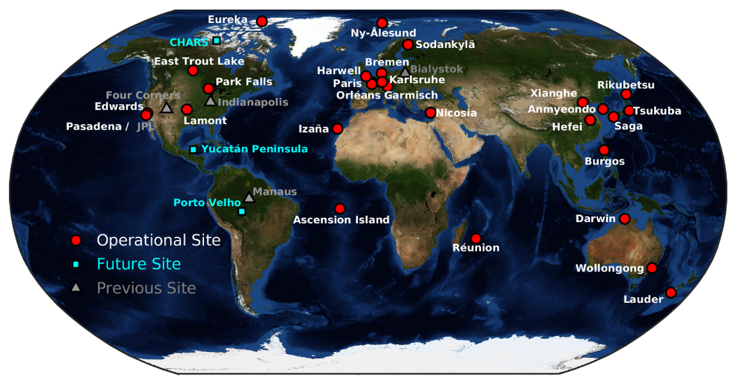
2.1.1. TCCON (Total Column Carbon Observation Network)

The Total Carbon Column Observation Network (TCCON) was established in 2004 as a ground-based network of Fourier Transform Spectrometers (FTS). These instruments record solar spectra to invert and monitor precision greenhouse gas data with the content of atmospheric molecules about CH₄, HF, CO₂, NO₂, etc. Since TCCON can provide accurate measurements (better than 0.25%) and inversion errors within 0.25% [16], the XCO₂ data measured by TCCON has been widely used to assess the accuracy of satellite retrievals, providing an essential data validation resource for GHG remote sensing satellites such as OCO-2 and GOSAT.

TCCON ground-based stations are strategically located around the world to provide long-term monitoring of atmospheric gases. The global distribution of these stations is depicted in Figure 4. In the figure, red dots denote active TCCON stations that measure atmospheric CO₂ column concentrations, grey dots indicate stations that have ceased operation, and bright blue dots represent proposed future sites. While these stations offer continuous time series data on atmospheric CO₂ concentrations, their sparse distribution limits the data to the regions surrounding each station, leaving gaps in the global and regional time series of CO₂ changes.

2.1.2. COCCON (COllaborative Carbon Column Observing Network)

KIT began constructing the COCCON (Collaborative Carbon Column Observing Network) using the portable FTIR spectrometer EM27/SUN in 2016 [15]. The EM27/SUN has a spectral resolution of 0.5 ${\mathrm{cm}}^{-1}$ (corresponding to a maximum optical path difference of 1.8 cm) and an acquisition time of approximately 58 s (the average time for 10 scans at a scanning speed of 10 kHz). It employs a DC-coupled InGaAs (indium gallium arsenide) detector and an extended InGaAs detector [17] to simultaneously observe various gas molecules, including CO₂, CH₄, CO, H₂O, O₂, N₂O, and HDO, within the frequency range of 4000–11,000 ${\mathrm{cm}}^{-1}$. The dual-channel observation mode covers the same spectral range used by TCCON and TROPOMI for short-wavelength inversion of CO and CH₄.

The COCCON network is designed to enhance greenhouse gas monitoring by addressing spatial and temporal gaps left by TCCON (Total Carbon Column Observing Network). By utilizing portable FTIR spectrometers like the EM27/SUN, COCCON accurately measures column concentrations of gases such as CO₂ and CH₄. The portability of COCCON’s instruments allows for flexible deployment in various environments, including remote and challenging areas, thereby extending the spatial coverage of greenhouse gas monitoring. The network provides high-resolution data, improves overall atmospheric observations, and collaborates with existing networks like TCCON to integrate data and enhance monitoring quality. Additionally, COCCON data supports the validation and improvement of satellite-based measurements and aids in climate change research and policy-making. Currently, nearly 100 EM27/SUN units are used by research teams worldwide for greenhouse gas research, including fixed-site concentration observation and field experiment emission estimation.

2.2. Satellite Remote Sensing Observations

Nowadays, satellite remote sensing detection technology is one of the most advanced means of obtaining CO₂ data. Sensors onboard satellites are used to acquire the spectral characteristics of atmospheric CO₂, which are then inverted by inversion algorithms to obtain CO₂ concentration data. Satellite remote sensing offers more continuous data compared to other observation instruments, with notable advantages such as continuity, uniformity, and wide coverage. Satellite observation methods for monitoring CO₂ concentrations are mainly divided into two types: one based on Thermal Infrared Radiation (TIR) detection, which is sensitive to CO₂ concentrations in the upper atmosphere and can provide vertical contour distributions of CO₂ using TIR spectra; the other based on Shortwave Infrared (SWIR) detection. The thermal infrared bands, sensitive to the mid to upper troposphere but less to near-surface CO₂ changes, contrast with shortwave infrared bands, which are sensitive to near-surface CO₂. Inversion channels are selected based on CO₂ absorption bands (strong: 15, 4.3, 2.06 µm; weak: 10, 5, 1.6, 1.4 µm) and are chosen according to regional and seasonal contexts. The primary inversion method uses the O₂-A band at 0.76 µm and CO₂ absorption bands at 1.61 µm and 2.06 µm to infer light scattering and related information. For detecting atmospheric CH₄, the method utilizes absorption near 1.65 µm. Inversion using the 1.65 µm and 2.06 µm bands retains over 90% of CH₄, CO₂, and temperature information, and more than 85% of H₂O information. Since both near-infrared and shortwave infrared are used for CO₂ inversion, the choice of wavelength range and spectral resolution is crucial. This decision depends on factors such as CO₂ absorption features, atmospheric sensitivity, spectral resolution requirements, atmospheric conditions, mission objectives, and sensor capabilities. Strong absorption bands such as 4.3 µm and 2.06 µm are typically used to improve measurement accuracy, while high spectral resolution helps differentiate closely spaced absorption features and enhances precision. However, the chosen bands also need to account for atmospheric factors like water vapor and the mission’s needs for temporal resolution and geographic focus. These factors collectively determine the final wavelength range and resolution to achieve accurate CO₂ measurements. Currently, operational satellites for detecting atmospheric CO₂ concentrations include GOSAT, SCIAMACHY, OCO-2, and TanSat.

In this paper, the development of carbon-monitoring technology is divided into three stages in Figure 5 based on the degree of progress of satellite remote sensing technology and the demand for carbon-monitoring applications: the initial stage (1996–2008), the rapid development stage (2009–2018) and the full-scale application stage (2019–present).

2.2.1. Development of Thermal Infrared Hyperspectral Sensors

The High-spectral Resolution Infrared Sensor (HIRS) developed in the 1970s in the United States marked a significant advancement in satellite remote sensing for atmospheric detection. Initially, infrared sensors were primarily used to monitor atmospheric temperature and humidity profiles. However, with advancements in sensor technology and inversion theory in atmospheric remote sensing, as well as the growing need to understand the atmospheric environment, thermal infrared hyperspectral sensors began to play a crucial role in atmospheric detection.

In August 1996, the Advanced Earth Observation Satellite (ADEOS) was launched, featuring the Interferometric Measurement of Greenhouse Gases (IMG) [18]. IMG was the first onboard hyperspectral Fourier sensor dedicated to gas detection via space-borne observations and demonstrated the feasibility of high-resolution sensors for detecting trace gases [19,20]. In May 2002, NASA’s Aqua satellite was launched, equipped with the Atmospheric Infrared Sounder (AIRS) and NOAA’s Advanced Microwave Sounder Unit (AMSU). AIRS was designed to enhance global climate research and weather prediction by improving the accuracy of tropospheric temperature profiles and atmospheric humidity measurements [21]. Subsequently, the Aura satellite, launched in June 2004, carried the high-resolution Tropospheric Emission Spectrometer (TES). In October 2006, the METOP-A satellite, part of the polar-orbiting meteorological satellite series, was launched with the next-generation hyperspectral atmospheric sounder, the Infrared Atmospheric Sounding Interferometer (IASI). In November 2017, China’s FY-3D satellite launched with the Hyperspectral Infrared Resolution Atmospheric Sounder (HIRAS) and the Greenhouse Gas Absorption Spectrometer (GAS). The following year, the GF-5 satellite was launched, featuring the Atmospheric Environment Infrared Ultraspectral Sounder (AIUS), the first occultation observational sensor with ultraspectral resolution in the infrared band developed by China.

Looking ahead, the Meteosat Third Generation (MTG) satellites will continue to contribute significantly into the 2040s. The MTG system will consist of two identical imaging satellites (MTG-I) with advanced capabilities and a sounding satellite (MTG-S) carrying an infrared sounder (IRS) and the Copernicus Sentinel-4 ultraviolet-visible and near-infrared instrument, marking the first deployment of such a system over Europe.

Table 1. Thermal infrared sensors for CO₂ detection.

Sensor	Mounting Platform	Launching Time	Spectral Type	Spectral Range	Spectral Resolution/cm−1	Spatial Resolution/km	Width/km
IMG	ADEOS	1996	Intervene	600∼3030 ${\mathrm{cm}}^{-1}$	0.15∼0.25	22	-
AIRS	EOS-Aqua	2002	Encoder	8.80∼15.4 µm	0.55	13.5	1650
				6.20∼8.22 µm	1.2
				3.74∼4.61 µm	2.0
TES	EOS-Aura	2004	Intervene	3.2∼15.4 µm	0.06	5	182
IASI	METOP	2006	Intervene	3.4∼15.5 µm	0.35∼0.55	12	2200
HIRAS	FY-3D	2017	Intervene	8.8∼15.38 µm	0.625	16	2250
				5.71∼8.26 µm	1.25
				3.92∼4.64 µm	2.5
AIUS	GF-5	2018	Intervene	750∼4100 ${\mathrm{cm}}^{-1}$	0.02	-	1850
IRS	MTG	2022	Intervene	8.26∼14.28 µm	0.625	4	-
				4.60∼6.25 µm		10

provides a summary of thermal infrared sensors used for CO₂ detection.

2.2.2. Development of Short-Wave Infrared Hyperspectral Sensors

The use of SWIR techniques to analyze atmospheric CO₂ has become a new approach with the continuous advancement of methods and means of space-based remote sensing observations. The reflection spectrum detected in the sensors carries information about the whole atmosphere and contains CO₂ information in the near-surface layer, Short-wave infrared sensors are mainly sensitive to the CO₂ concentration near the surface and are often used to invert the column concentration of atmospheric CO₂. Sensors that utilize the short-wave infrared band (1.6 µm) for the inversion of CO₂ mainly include SCIAMACHY, GOSAT, OCO-2, and TanSat.

European Satellites

The European polar-orbiting Earth observation satellite Envisat-1, launched on 1 March 2002, carried the Scanning Imaging Absorption Spectrometer for Atmospheric Charting (SCIAMACHY), the world’s first satellite sensor capable of measuring carbon dioxide and methane concentrations. SCIAMACHY has three modes of observation: limb, nadir, and occultation, with a spatial resolution of 30 km × 60 km.

Japanese Satellites

The GOSAT satellite, launched by Japan in 2009, was a pioneering mission for greenhouse gas monitoring, utilizing the Thermal and Near Infrared Sensor for carbon Observation Fourier-Transform Spectrometer(TANSO-FTS) and the Cloud and Aerosol Imager (CAI) instruments to measure global CO₂ and CH₄ concentrations. Its data products are categorized into four levels, from raw spectral data (Level 1) to global CO₂ fluxes (Level 4). GOSAT’s spatial resolution is 10 km × 10 km with a re-observation period of 3 days. The GOSAT-2, launched in 2018, improves upon this with enhanced TANSO-FTS-2 and CAI-2 instruments for more precise measurements.

United States Satellites

In 2009, NASA launched the Orbiting Carbon Observatory (OCO), the first satellite dedicated to high-precision, global CO₂ measurements, but it failed that year. In 2014, OCO-2 successfully launched, equipped with a single payload that integrates three high-resolution grating spectrometers. OCO-2 features a spatial resolution of 1.29 km × 2.25 km and revisits locations every 16 days. Its data products include: the primary class contains all the collected soundings; the secondary class has atmospheric CO₂ column concentration, surface albedo, and aerosol content; the tertiary product consists of the global CO₂ concentration maps; the quaternary product is the global CO₂ source/sink carbon fluxes.

In 2019, OCO-3 was launched aboard the International Space Station (ISS). It offers enhanced CO₂ and Solar-Induced Fluorescence (SIF) observations with a broader range and better capability for local and point source measurements [22].

China Satellite

In 2016, China launched the TanSat satellite, which is the third international satellite dedicated to high-precision greenhouse gas detection. TanSat is equipped with two main instruments: Atmospheric Carbon Dioxide Grating Spectrometer (ACGS) and Cloud and Aerosol Polarisation Imager (CAPI). The satellite’s primary goal is to monitor global CO₂ concentrations with high spatial and spectral resolution, covering the entire world, China, and other key regions. The top-tier product from TanSat is the radiospectral data, with CO₂ inversion accuracy of 1% (1–4 ppm). The Institute of Atmospheric Physics of the Chinese Academy of Sciences developed a high-precision inversion algorithm called IAPCAS, which was used to generate the first global CO₂ distribution map from TanSat’s data as Figure 6 shown [23].

Following TanSat, China launched the Fengyun-3D (FY-3D) and Gaofen-5 (GF-5) meteorological satellites after 2017. These satellites primarily measured column concentrations and global distribution changes of CO₂ and CH₄. In 2021, China further advanced its capabilities with the launch of the hyperspectral observation satellite GF5-02, which carries the GMI payload for enhanced measurements.

Planned Future Launches of Remote Sensing Satellites CO₂

In the future, several CO₂ observing satellites are planned for launch.

The next-generation satellite in the GOSAT series, GOSAT-GW (Global Observing Satellite for Greenhouse Gases and the Water Cycle), will launch after 2024. It will carry the TANSO-3, a third-generation thermal infrared and near-infrared carbon-observation grating imaging spectrometer, offering better spatial coverage of greenhouse gases concentrations and addressing the continuous detection limitations of GOSAT and GOSAT-2.

The MicroCarb mission, a French-British satellite collaboration, aims to launch in early summer 2025. It will monitor CO₂ exchanges between sources and sinks, with a 13.5 km strip width, 4.5 km (in cross-tracks) × 9 km (along-tracks) spatial resolution, and a 21-day repeat cycle. The European Space Agency’s Copernicus Anthropogenic CO₂-Monitoring Mission (CO₂M) program, starting in 2025, will consist of two satellites. Its main instrument, the Infrared Spectrometer (ISI), features a 2 km × 2 km resolution and a 250 km wide observational bandwidth [24] with simultaneous imaging observational capability for monitoring anthropogenic CO₂ emissions.

The Carbon Mapper Coalition, in collaboration with public and private partners, announced on 15 April 2021, its plan to deploy an innovative hyperspectral satellite constellation designed to pinpoint, quantify, and track point-source methane and CO₂ emissions. Phase 1, currently underway, involves the development of the first two satellites by Planet and NASA’s Jet Propulsion Laboratory (JPL), also a member of the Carbon Mapper Coalition, with a planned launch in 2024. Phase 2, in development, will expand into an operational multi-satellite constellation starting in 2025. On 16 August 2024, the Carbon Mapper Coalition launched Tanager-1, the first satellite of Phase 1, to improve transparency regarding methane and CO₂ super-emitters and encourage global action. Tanager-1 is equipped to detect, locate, and measure these super-emitters from space. JPL also plans to launch a second Tanager satellite later, which will be outfitted with an imaging spectrometer developed by JPL.

China expects to launch the second-generation carbon satellite (TanSat-2) in 2025. TanSat-2 is a satellite cluster consisting of two to three satellites measuring XCO₂ at an across-track swath of 2900 km and with a pixel size of 2 km × 2 km. TanSat-2 will add the short-wave infrared channel of 2.305∼2.385 µm to the first-generation carbon satellite (TanSat) for CH₄ and CO detection. The precision of its XCO₂ measurements is expected to be less than 1 ppm, which effectively improves the spatial and temporal coverage and global detection capability. It is intended to verify satellite data using ground-based measurements from the Total Carbon Column Observing Network and EM27/SUN measurements for optimizing parameters in satellite sampling.

The summary of typical shortwave infrared satellites and sensors is presented in

Table 2. Summary of typical shortwave infrared satellites and sensors (by time).

Country	Satellite	Detection Payload	Launching Time	Spatial Resolution/km	Spectral Band/µm	Spectral Resolution/cm−1	Width/km
European Union	ENVISAT-1	SCIAMACHY	2002–2003	30 × 60	0.24∼2.4	4.2	960
Japan	GOSAT	TANSO-FTS/CAI	2009–2001	10.5	0.76∼14.3	0.6/0.27	640
United States	OCO-2	3-band grating hyper spectrometer	2014–2007	1.29 × 2.25	0.76∼2.08	0.043/0.083/0.104	10.6
China	TANSAT	ACGS/CAPI	2016–2012	2 × 2	0.76∼2.08	0.044/0.125/0.165	18
China	FY-3D	GAS/FTS	2017–2011	10	0.75∼2.38	0.6/0.27	2250
China	GF-5	GMI	2018–2005	10.3	0.76∼2.06	0.6/0.27	865
Japan	GOSAT-2	TANSO-FTS-2/CAI-2	2018–2010	9.7	0.76∼14.3	0.6/0.27	632
United States	OCO-3	3-band grating hyper spectrometer	2019–2005	1.6 × 2.2	0.76∼2.08	0.044/0.084/0.108	10.6
China	GF-5-02	GMI	2021–2009	10.3	0.76∼2.06	0.6/0.27	865
France	MicroCarb	Infrared spectrometer	2025	4.5 × 9	0.76∼2.06	-	13.5
United States	Carbon Mapper	Hyperspectral imaging spectrometer	2024	0.03	0.4∼2.5	0.05	18
Japan	GOSAT-GW	TANSO-3	2024	10/1∼3	0.45∼1.6	0.05/0.02	911/90
European Union	CO2M	CO2I/NO2I	2025	2 × 2	0.74∼2.09	0.12/0.3/0.35	256
China	TANSAT-2	-	2025	2 × 2	-	-	—

below.

2.3. CO₂ Observation Database

2.3.1. XCO₂ Products

A global team of researchers uses meteorological observation stations, satellite remote sensing, and ground monitoring to create a high-resolution global dataset of near-surface greenhouse gas (GHG) observations. They compare this data with the Total Carbon Column Observing Network (TCCON) [25] and develop inversion algorithms for accuracy. Current XCO₂ products from satellites (GOSAT-2, TanSat, OCO-2) are processed using the RemoTeC full-physics algorithm, UoL FP algorithm, FOCAL algorithm, and IAPCAS algorithm. These datasets and algorithms are publicly available, with updates and data range extensions made annually [26].

The latest XCO₂ product information for specific remote sensing satellites is shown in

Table 3. XCO₂ product information for remote sensing satellites.

Data Name	Algorithm	Version	Time Range	Download Website
SCIAMACHY WFMD	WFM-DOAS	V4.0	10.2002–04.2012	[27]
SCIAMACHY BESD	DOAS-BESD	V2.1.2	01.2003–03.2012	[28]
GOSAT OCFP	UOL-FP	V7.0	04.2009–12.2015	[29]
CO2_EMMA	EMMA	V2.2	06.2009–06.2014	[30]
GOSAT-2 ACOS	ACOS	V9r	04.2009–08.2020	[31]
GOSAT-2 SRFP	RemoTeC	V2.0.0	02.2019–08.2020	[32]
GOSAT-2 NIES	NIES	V2.95	04.2009–08.2020	[33]
Tansat OCFP	UOL-FP	V1.2	11.2017–12.2020	[34]
OCO-2 ACOS	ACOS	V11.1r	09.2014–08.2024	[35]
OCO-2 FOCAL	FOCAL	V10	09.2014–05.2021	[36]
OCO-3 ACOS	ACOS	V10.4r	08.2019–08.2024	[37]

. Certain data products and releases are still undergoing updates.

2.3.2. Anthropogenic Emissions Dataset

Anthropogenic emission data is crucial for estimating the concentration of CO₂ in the atmosphere. This data encompasses emissions from a variety of human activities that contribute to the global carbon footprint. The primary sources of anthropogenic CO₂ emissions come from agricultural activities, industrial production, land use changes, and waste disposal, and are monitored and verified through carbon accounting, climate modeling, and emissions inventories.

ODIAC Dataset

ODIAC, launched by JAXA in 2008, is a global high-resolution dataset for CO₂ emissions from fossil fuel combustion. Its primary aim is to provide foundational information on fossil fuel CO₂ emissions for global and regional flux inversions using GOSAT observations [38]. ODIAC estimates CO₂ emissions by combining spatial allocations of point source locations with nighttime lighting data from power plants around the world. The dataset provides global monthly emissions information with spatial resolutions of 1 km × 1 km and 1° × 1°.

The data can be seen from the website https://db.cger.nies.go.jp/ (accessed on 30 July 2023).

EDGAR Dataset

EDGAR, published by the Joint Research Centre of the European Commission, provides independent estimates of global anthropogenic emissions and trends [39]. It relies primarily on population density data to map emissions spatially. The EDGAR methodology is bottom-up and sectoral, utilizing statistical estimates of CO₂ emissions from various sectors, including industrial facilities. This approach considers factors such as population distribution and land use types to estimate emissions accurately.

The data can be seen from the website https://edgar.jrc.ec.europa.eu/ (accessed on 13 May 2023).

MEIC Dataset

MEIC (Multi-resolution Emission Inventory for China) is a detailed emission inventory for China, providing emissions data at various resolutions [40], including CO₂ and other greenhouse gases. It integrates multiple data sources such as remote sensing data, ground observations, and statistical data to enhance the accuracy of emission estimates. The MEIC model categorizes emission sources into different types, such as energy, industry, and agriculture, offering detailed information on regional and temporal scales. This dataset is crucial for climate change research, policy-making, and environmental monitoring.

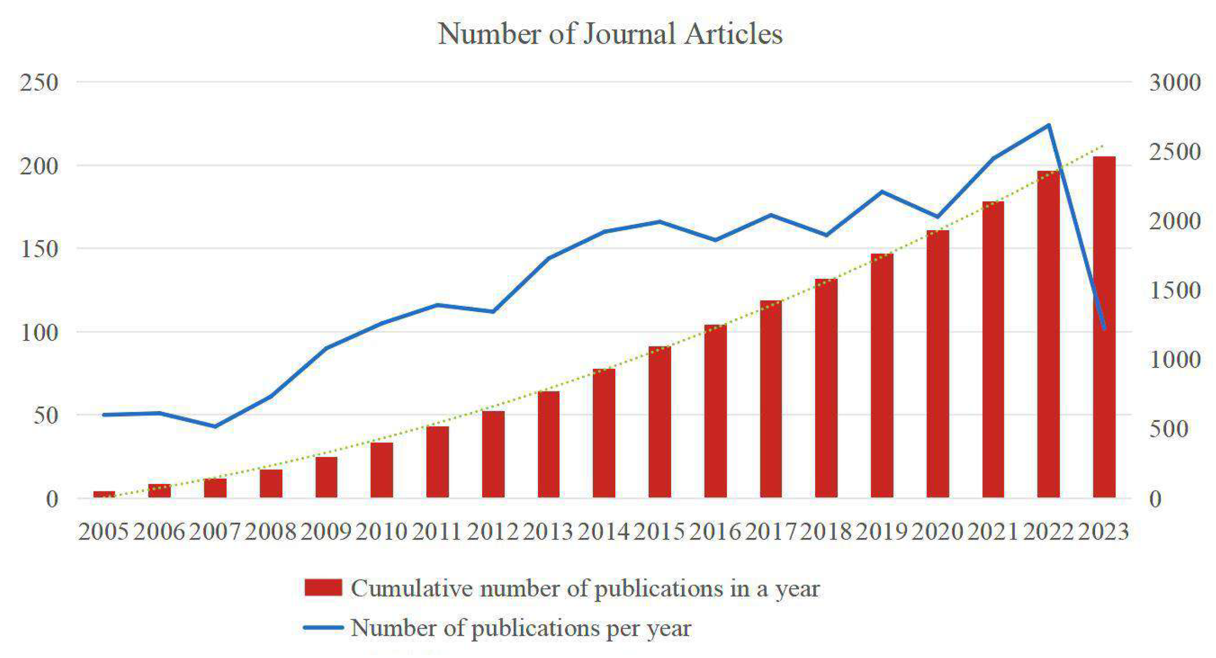
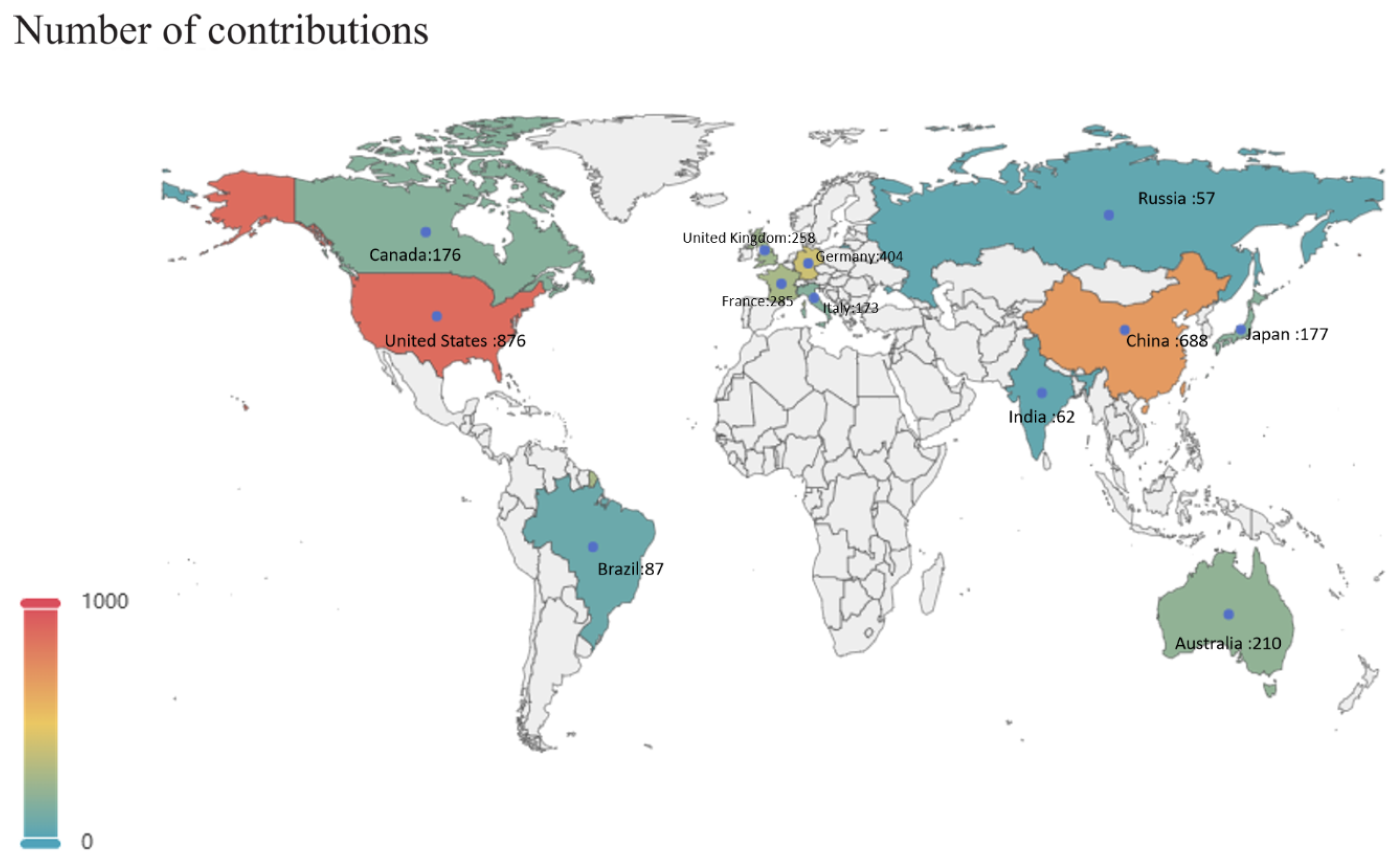
2.4. Citespace-Based Global Research

In this section, Citespace [41,42] software v6.2.4 is used to analyze and visualize literature on global carbon inversion assimilation, focusing on keyword mapping and author contributions, etc. The goal is to outline research activities and trends over the past 20 years in this field. The analysis, based on a Web of Science search with keywords such as satellite remote sensing, carbon inversion, data assimilation, and XCO₂, covers the period from 2005 to 2023 with yearly time slices. Approximately 2000 significant articles were exported for this study. The results include plotted and analyzed data on publication numbers, keywords, national institutions, and research topics.

Figure 7 illustrates the annual number of publications on satellite remote sensing CO₂ and inverse assimilation from 2005 to mid-2023. The blue line shows the yearly publication count, peaking in 2022, while the red bar graph represents the cumulative number of publications, indicating an upward trend. This figure highlights the increasing investment and attention in carbon remote sensing research.

Figure 8 presents a keyword heat map based on approximately 2000 paper articles. The size of the circles corresponds to the frequency of keyword appearance, and the connecting lines indicate relationships between different keywords. Notably large circles for “atmospheric CO₂”, “satellite remote sensing”, “inverse assimilation”, and “modeling” highlight their prominence. This indicates a strong link between CO₂ inversion and satellite remote sensing. Additionally, recent trends include emerging technologies such as satellite inversion, machine learning, and data assimilation, reflecting current hot topics in carbon remote sensing.

Figure 9 displays a map showing the number of publications on satellite-based carbon dioxide remote sensing by national institutions. In this map, larger circles represent higher publication frequencies and greater contributions. Nodes highlighted in red indicate areas of significant attention in the field. The graph reveals that prominent institutions and laboratories from the United States, China, the United Kingdom, and Germany have made substantial contributions to this research area.

This paper employs the Pycharts module in Python to create a flat world map illustrating contributions from different countries to carbon remote sensing research. Figure 10 uses various colors to represent the level of contributions, with grey indicating no contributions from certain regions among around 2000 papers. The map shows that the United States, China, the United Kingdom, and Germany are leading in this field. Other countries are emerging, and increased attention and investment in carbon neutrality are expected to accelerate global progress.

2.5. Section Summary

This section summarizes ground observation and space carbon satellite observation methods. The part gives a detailed introduction to the development of satellite remote sensing sensors and techniques. Additionally, this subsection introduces relevant datasets, incorporating those from carbon satellites and anthropogenic emissions. Finally, the section employs the Citespace visualization tool to showcase recent papers on carbon-emission research in terms of regions, keywords, and topic clustering. Section 3 spotlights the retrieval algorithm of the column concentration of atmospheric CO₂ in satellite observations.

3. Carbon Satellite Remote Sensing Inversion Techniques

Atmospheric components have different sensitive bands for spectral absorption, scattering, and refraction. Based on the inversion theory, the relationship between the concentration of the target gas and the satellite-observed atmospheric absorption spectra can be expressed as a complex nonlinear function, and its mapping relationship includes the effects of emission surface characteristics, temperature, clouds, and the radiative branching of the aerosol contribution. It is also affected by the spectral response function, spectral resolution, and radiative noise associated with the effects related to instrumental characteristics. Obtaining information on atmospheric parameters from these measurements for meteorological applications requires “inversion” of the observational process or “direct assimilation” of the radiative intensity data into numerical atmospheric models. The first step is to understand the basic theory of atmospheric radiative transfer and the methods of its calculation, and on this basis to establish an accurate model describing the process of radiative transfer in the atmosphere, to provide the basis and conditions for the development of inversion algorithms.

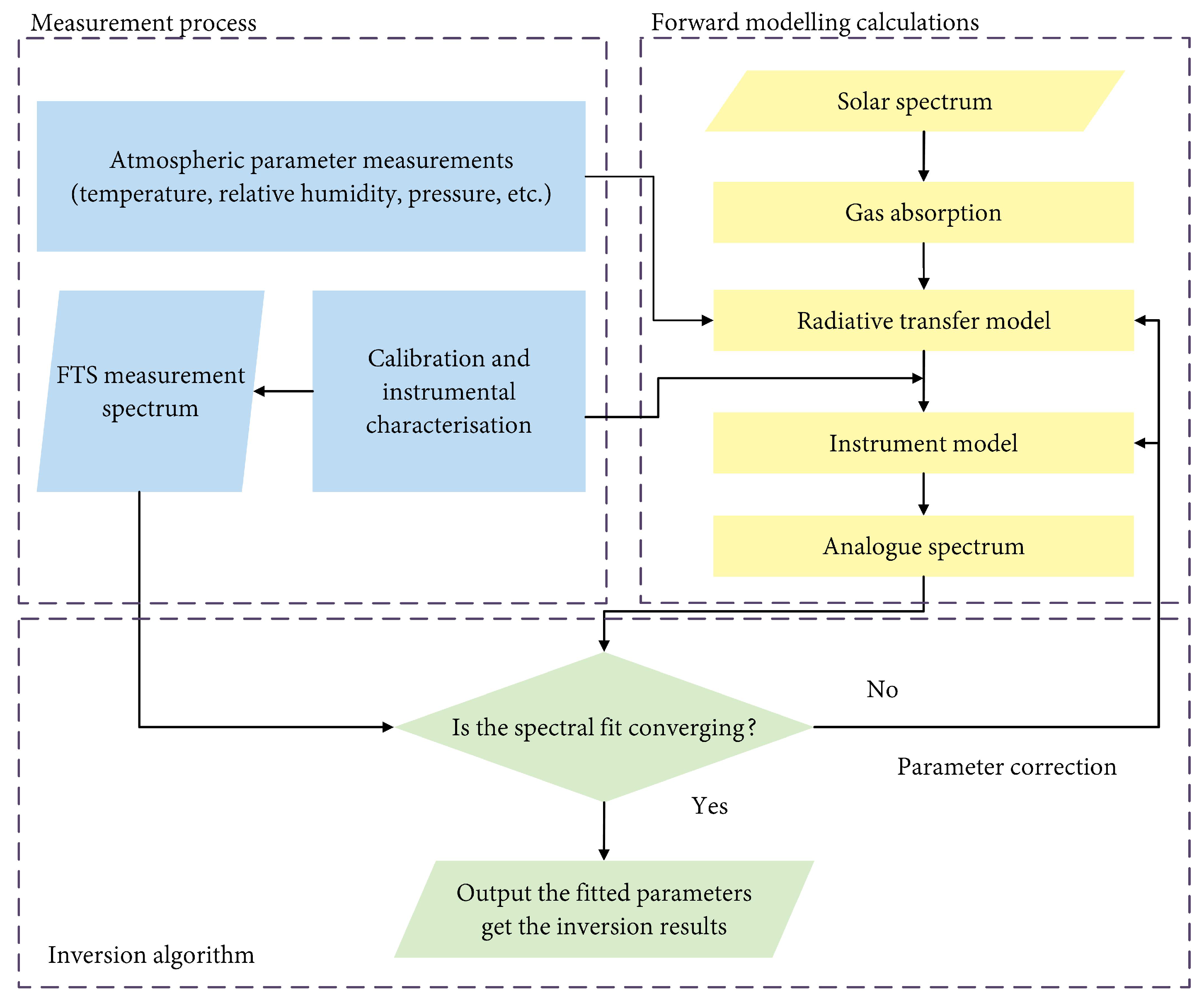
3.1. Orthogonal Modelling and Inversion Principles

3.1.1. Basic Principles of Remote Sensing Inversion

The ultimate goal of satellite remote sensing observations is to analyze and calculate the physical and chemical properties of the atmosphere or target from spectra or images observed by satellite instruments, and to use these input parameters as information about the actually observed atmosphere. To achieve this, appropriate inversion algorithms are required. The main components of remote sensing inversion are the forward model, the inversion method, and the error analysis. The forward model is the basis of the inversion algorithm. The forward process of satellite remote sensing describes the physical process between atmospheric covariates to observations, using the physical process of radiative transfer to simulate the radiant brightness of the sensor and returning a spectrum of simulated radiances and the partial derivatives of these radiances concerning some of the atmospheric and surface state attributes, which also referred to as Jacobi determinants. The Jacobi matrix is used in the inversion process to estimate the state covariates required to minimize the difference between the observed and simulated spectra. The assumed atmospheric state is modified to improve the fit to the measured spectra by controlling the margin of error between the two sides by solving for residuals, and the process is repeated until convergence conditions are met. Once the atmospheric state that produces the best fit to the observed spectrum is found, the algorithm determines the errors from different sources (e.g., vertical smoothing, measurement noise, etc.) in XCO₂, XCO2, and the XCO₂ column-averaged kernel function (CAK), and obtains the corresponding atmospheric state results. The relationship between the atmospheric composition measurements, the forward model, and the inversion algorithm is shown in Figure 11.

The closer the description of each part of the forward model is to the actual situation, the more accurate the simulated spectra will be, and the higher the accuracy of the inversion based on this fitting will be. The inversion algorithm is based on the mapping relationship provided by the forward model to find the optimal set of conditions from all possible states, so that the simulation results of the forward model are the closest to the actual results of the instrument, and the inversion value is obtained at this time.

Combined with the satellite observation model, considering the solar radiation and the satellite instrument modeling function, the forward process can be expressed as follows:

$$y=F(x,b)+\epsilon$$

(1)

where y is the measurement vector, x is the inverse state vector, b is the non-inverse state vector, and $\epsilon$ is the error vector. F(x,b) is a function of the state vector as the forward model, which describes the entire physical process of the measurement. The input parameters to the a priori state vector consist of atmospheric parameters and the observed spectra, and the cost function represents the cost of different minimum deviations by optimizing the difference between the measured and simulated spectra as well as the difference between the state vector and the a priori information. The solution equation can be used to minimize the bias cost function by means of an optimization algorithm [43].

$$J\left(x\right)={[F\left(x\right)-y]}^T{S}_{\epsilon }^{-1}[F\left(x\right)-y]+{(x-x_a)}^T{S}_a^{-1}(x-x_a)$$

(2)

where $S_a$ is the a priori error variance matrix, $x_a$ is the a priori state vector, $S_{\epsilon }$ is the error covariance matrix, and T denotes the matrix transpose matrix. XCO₂ can be computed directly from the x of the cost function formulation, where the forward model is rerun at each iteration in the minimization of the cost function solver, but needs to use the a priori information gained in the previous iteration. The improved state vector x formula is as follows:

$$x_{i+1}=x_i+{(K_i^T{S}_{\epsilon }^{-1}{K}_i+(1+\gamma )S_a^{-1})}^{-1}[K_i^T{S}_{\epsilon }^{-1}(y-F\left(x_i\right))+S_a^{-1}(x_a-x_i)]$$

(3)

where $F\left(x_i\right)$ is the forward model at $x_i$, $K_i$ = ${\displaystyle \frac{\partial F\left(x_i\right)}{\partial x_i}}$ corresponds to the Jacobi matrix, and $\gamma$ is the Levenberg-Marquardt parameter. The process is iterated until the set $\gamma$ convergence condition is satisfied, details of which are given by Crisp et al. [44]. In the inversion process, the profile concentration of CO₂ on the gas column is obtained. In order to calculate the XCO₂, one more step is required with the equation

$$XC{O}_2=h^T\widehat{u}$$

(4)

where $\widehat{u}$ is the CO₂ concentration profile inverted over a fixed pressure layer and h is the pressure weighting parameter [45].

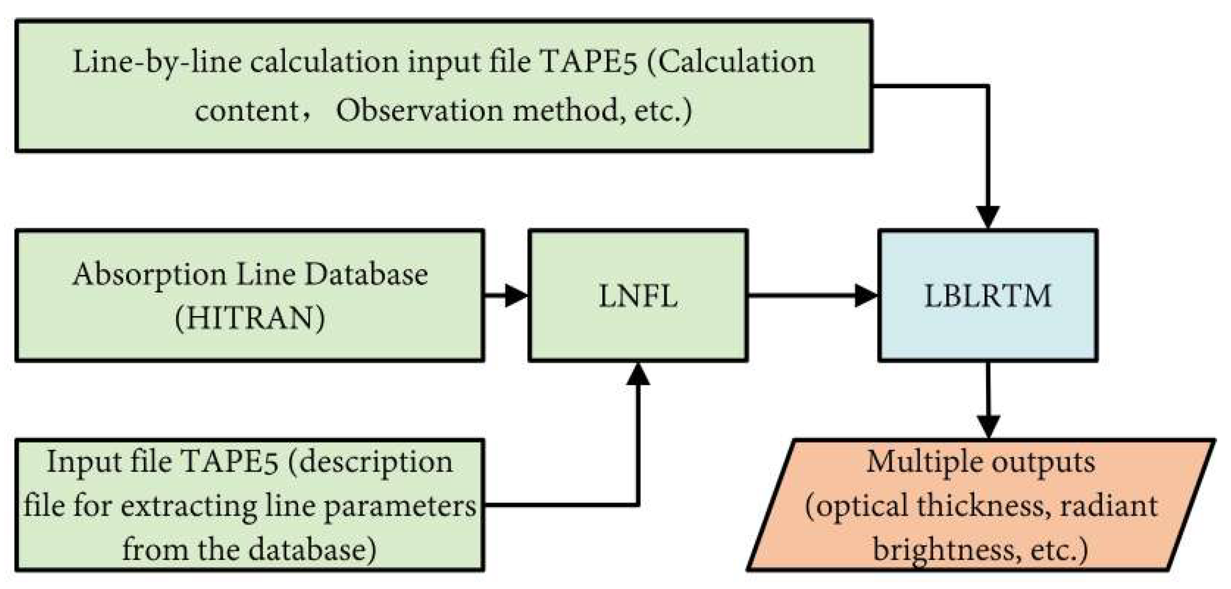
3.1.2. Selection of Forward Modelling

In hyperspectral satellite remote sensing, the forward model is a numerical simulation model that describes the remote sensing observation process of a satellite instrument. The radiative transfer model is the core of the forward model, and the concentration inversion is based on the molecular absorption features generated during the radiative transfer process. As an important component of the forward model, the model is designed to simulate the full physicochemical processes of the atmospheric radiation field, which include the properties of incident sunlight, its transmission, reflection, refraction, scattering, and radiation in the atmosphere, as well as thermal radiation from the ground and bi-directional surface reflections. Theoretically, the intensity of radiation observed by satellite instruments at the top of the atmosphere can be fully determined by these parameters and boundary conditions when a certain observational coordinate system is established.

Atmospheric radiative transfer model calculation parameters generally include absorption, emission, and scattering. The following are descriptions and principles of several atmospheric radiative transfer models:

4A/OP: It is a physical radiative transfer model developed by the LMD Laboratory based on a fast line-by-line integration model. It can be used to simulate atmospheric absorption and scattering for the thermal infrared spectral region. It contains a database of atmospheric absorption GEISA [46] constructed using a wavelength-by-wavelength, layer-by-layer model. With this database, 4A allows the calculation of direct transmittance in each layer of the atmosphere and the calculation of radiation at different altitudes.

6S: The 6S model was developed by Vermote et al. [47] of the University of Maryland, USA, in 1997 based on the 5S. The 6S model consists of the following five main parts: the sun, the geometrical relationship between the features and sensors, the atmospheric model, the aerosol model and spectral properties of sensors, and the reflectance of the ground surface. The solving of the radiation equations takes into consideration the multiple scattering and the interactions between the molecular scattering and the aerosol scattering. The 6S model mainly serves the MODIS atmospheric correction algorithm, which can accurately simulate satellite observations in the visible band.

LOWTRAN: LOWTRAN 7 is a single-parameter, spectral band mode atmospheric transport model developed by the American Geophysical Laboratory, which is a software package for calculating atmospheric transmittance and radiation, and supplemented by molecular line parameters obtained from theoretical calculations. LOWTRAN mainly consists of three algorithms: multi-scattering processing, transmittance calculation, and geometric paths of light rays, which are fast in calculation speed and widely applied for modeling atmospheric forcings and backgrounds. However, it also has inherent defects, such as the two-stream approximation for dealing with scattering problems limits its computational accuracy, and the direction-dependent irradiance calculation is not highly accurate.

MODTRAN: MODTRAN is an atmospheric radiative transfer model developed by the United States Air Force, which is an improved model of LOWTRAN with the basic structure and framework of the program remaining intact, and the absorption band mode parameters calculated using the latest HITRAN database. In addition, by further refining the wave number interval of the K-distribution, the latest version of MODTRAN 5.0 has improved the spectral resolution to 0.1 ${\mathrm{cm}}^{-1}$.

SCIATRAN: An integrated atmospheric radiative transfer and inversion model developed by the University of Bremen, Germany, for SCIAMACHY. It is based on GOMETRAN and can calculate atmospheric radiative intensity, weight function, atmospheric mass, column concentration, and radiative flux simultaneously. It is applied to limb, sky, and occultation observation modes and contains solar spectral data, absorption cross-section data of various atmospheric components, and vertical profile data of atmospheric trace components, as well as aerosol and surface albedo data. However, the range of bands it supports is only 175.44∼2400 nm covered by SCIMACHY.

LBLRTM: LBLRTM v12.1 is an atmospheric radiative transfer model developed by Lawrence Berkeley National Laboratory, based on FASCODE developed by the US Air Force Phillips Laboratory, with improved design and higher computational accuracy. LBLRTM is capable of handling a wide range of gases and aerosols, taking into account atmospheric absorption, scattering, and transmission, and is widely used in the fields of atmospheric chemistry and remote sensing. The LBLRTM radiative transfer software package includes LNFL, a tool for atmospheric spectral line parameterization, and LBLRTM, the radiative transfer calculation component, as documented in Figure 12.

VLIDORT: It is used to simulate the transport process of solar radiation in the atmosphere by vector radiative transfer model based on the discrete coordinate method. Rayleigh scattering of molecules is simple in form and can be calculated directly and accurately by the formulae, which are developed based on the LIDORT radiative transfer model.

DISORT: DISORT is an atmospheric radiative transfer model developed at the University of Illinois at Urbana-Champaign, IL, USA. The main features of DISORT are high computational speed and accuracy, its ability to deal with multi-layer atmospheres and multiple gases, and wavelength coverage ranging from UV to microwave, which includes the physical processes of absorption, scattering, and thermal radiation, as well as bi-directional reflections and emissions at the lower boundary.

RTTOV: RTTOV is a fast radiative transfer model developed and more widely used based on the radiative transfer model of the European Centre for Medium-Range Numerical Weather Forecasts (ECMWF) simulation of the TOVS satellite observations. RTTOV is mainly characterized by high accuracy, fast computation speed, and its ability to deal with a wide range of gases and clouds, and it has been applied to the inversion process of the thermal infrared wavelengths of the satellite CO₂ gases.

LINTRAN: LINTRAN v2.0 is a linearised vector radiative transfer forward model used in famous algorithm RemoTAP, employing forward-adjoint theory, that is capable of modelling cloud contaminated satellite observations and their derivatives with respect to the state of the atmosphere and the Earth’s surface in a numerically efficient manner. Compared to LINTRAN v1.0, v2.0 improves efficiency by combining an iterative solving method with forward-adjoint perturbation theory and separating the first N orders of scattering from the diffuse intensity vector field. LINTRAN is instrumental in analyzing spectral features for identifying and quantifying atmospheric trace gases.

Table 4. Common radiative transfer models.

Radiative Transfer Model	Band Range	Absorption Calculation Methods	Scattering	Polarization	Reference
4A/OP	Near Infrared∼Thermal Infrared	Line by line	Supported	Supported	[48]
6S	Visible Wave	Band pattern	Supported	Supported	[47]
LOWTRAN	50,000 ${\mathrm{cm}}^{-1}$∼Microwave	Band pattern	Supported	Unsupported	[49]
MODTRAN	50,000 ${\mathrm{cm}}^{-1}$∼Microwave	Band pattern/K-distribution	Supported	Supported	[50]
SCIATRAN	Ultraviolet∼Near Infrared	Line by line	Supported	Supported	[51]
LBLRTM/FASCODE	Ultraviolet∼Millimeter Wave	Line by line	Unsupported	Unsupported	[52]
VLIDORT	Ultraviolet∼Microwave	/	Supported	Supported	[53]
DISORT	Ultraviolet∼Microwave	/	Supported	Supported	[54]
LINTRAN	Visible Wave∼Thermal Infrared	Line by line	Supported	Supported	[55]
RTTOV	Near Infrared∼Thermal Infrared	Line by line	Supported	Unsupported	[56]

displays the common radiative transfer models.

3.2. Advances in Remote Sensing Algorithms for Satellite Atmospheric CO₂

The principle of satellite remote sensing inversion of CO₂ is mainly to use the radiation spectra near the absorption band of CO₂ measured by the detector to invert and calculate the concentration of CO₂ column. The choice between profile inversion and column concentration inversion algorithms depends on specific needs and data availability. Profile inversion is used when detailed vertical distribution information is required, such as in-depth studies of vertical mixing in the atmosphere or emission sources at specific heights. This method provides high-resolution vertical data but is complex and data-intensive. In contrast, column concentration inversion is suitable for cases where detailed vertical data is less critical or not available. It provides an overall estimate by integrating concentration data across the entire column, simplifying the inversion process and making it suitable for large-scale assessments and general monitoring.

The CO₂ inversion algorithms mainly include two categories, namely, empirical algorithms and physical inversion algorithms, in which the physical methods are based on the radiative transfer model with the advantages of high precision, universality and quantitative estimation of errors; the empirical statistical methods, which have the advantage of high-speed computation, are generally used in inversion scenarios that have a high time limit and a lower demand for precision. Besides, new data-assimilation algorithms have been applied to satellite data inversion. Atmospheric CO₂ column concentrations obtained from CO₂ satellite observations and satellite remote sensing inversion algorithms, combined with atmospheric transport models and atmospheric inversion algorithms, have been used to assess terrestrial carbon sinks.

3.2.1. Physical Inversion Algorithms

DOAS Algorithm

The conventional Differential Optical Absorption Spectroscopy (DOAS) algorithm was first proposed by Platt et al. [57], which mainly focused on the UV-visible band (200∼760 nm) for the inversion of trace gases in ground-based observations, but the algorithm introduces large errors in the inversion of infrared bands. Buchwitz et al. [58,59,60] developed the WFM-DOAS algorithm based on the DOAS algorithm, which was applied to the inversion of SCIAMACHY near-infrared spectra for atmospheric CO₂ column concentrations. WFM-DOAS is an unconstrained linear least squares method based on the scaling (or shifting) of preselected vertical profiles, and it obtains information on atmospheric CO₂ by matching the logarithms of irradiance of the observed spectrum to the simulated spectrum. The effect of the slow variations in the spectra is removed by the differential absorption. The WFM-DOAS algorithm, with accurate calibration of the observed spectra, performs a first-order Taylor expansion of the natural logarithm of the solar normalized radiation intensity at the wavelength ${\lambda }_i$, expressed as:

$$\begin{array}{c}\hfill ln{I}_i^{means}(V^t,b^t)\approx ln{I}_i^{mod}(\overline{V},\overline{b})+{\displaystyle \frac{\partial ln{I}_i^{mod}}{\partial V_j}}{\mid }_{\overline{V}}\times (\widehat{V}-\overline{V})+\\ \hfill {\displaystyle \sum _{j=1}^F}{\displaystyle \frac{\partial ln{I}_i^{mod}}{\partial b_j}}{\mid }_{\overline{b_j}}\times (b_j-{\overline{b}}_j)+P_i\end{array}$$

(5)

where $I_i^{means}$ and $I_i^{mod}$ are the observed and simulated values of normalized radiation intensity at ${\lambda }_i$, and $V^t$, $\overline{V}$ and $\widehat{V}$ are the true, simulated, and inverted values of the total column of atmospheric components respectively. $b_j$ represents atmospheric temperature, pressure, aerosol, cloud parameters and surface albedo, etc., $P_i$ is a low-order polynomial. Then the simulated spectral constants and column weight functions normalized by the sun can be obtained by the atmospheric radiative transfer simulation software SCIATRAN (V4.6) calculations, and the vertical column concentrations of the inverse-performing gases are based on the least-squares fitting of the spectra to the observed spectra:

$${∥ln{I}_i^{means}(V^t,b^t)-ln{I}_i^{mod}(\overline{V},\overline{b})∥}^2\equiv {∥RE{S}_i∥}^2⟶min$$

(6)

In overview, the WFM-DOAS implementation process [61] is shown in Figure 13.

The initial WFM-DOAS inversion faced challenges due to its inability to address aerosol scattering effects and its low accuracy [62]. To correct for temperature and pressure dependencies of gas absorption cross-sections in the infrared spectrum, various international research groups have developed improved inversion algorithms based on conventional DOAS principles. For example, Frankenberg et al. [63] from the University of Heidelberg developed the IMAP-DOAS algorithm, an enhanced iterative maximum a posteriori probability DOAS method for SCIAMACHY. Barkley et al. [64] further refined this approach with the Full Spectral Initiation (FSI)-WFM-DOAS algorithm, which incorporates an a priori profile with actual atmospheric parameters and accounts for three aerosol modes, increasing computational complexity. Schneising et al. [65] and Oshchepkov et al. [66] improved the WFM-DOAS algorithm by including SCIAMACHY’s M-factor, a multiplicative correction related to absolute radiative calibration, which reduced errors from aerosol and cloud scattering. This enhanced algorithm improved the accuracy of XCO₂ concentration retrieval over long time series and expanded SCIAMACHY’s applicability to non-clear-sky conditions. Additionally, WFM-DOAS has been further enhanced with constant aerosol vertical profiles and cloud-detection algorithms in radiative transfer simulations [67]. Heymann et al. [68] from the University of Bremen developed the BESD algorithm, which integrates optimal estimation with WFM-DOAS to retrieve CO₂ from SCIAMACHY and GOSAT L1B open data.

Optimal Estimation Algorithm

Optimal estimation algorithms need to determine the cost function first and then use different optimization strategies to minimize the cost function.

The National Institute for Environmental Studies (NIES) of Japan developed the NIES-FP inversion algorithm using an optimal estimation approach. This algorithm retrieves the column abundances of CO₂ and CH₄ from short-wavelength infrared spectra collected by the TANSO-FTS [69]. It features an unbiased cloud-detection algorithm [70] that utilizes the TANSO-CAI cloud product for cloud screening and refines the atmospheric light path by simultaneously inverting aerosol, surface, and gas parameters at observational pixels. As the standard algorithm for GOSAT data products, it has demonstrated high accuracy in GHG inversions, achieving errors within 1% [71]. Recently, Someya et al. [72] introduced a new version, V03.xx, of the NIES SWIR L2 product algorithm.

The ACOS retrieval algorithm, initially developed by NASA’s science team for the OCO satellite, was adapted for use with the GOSAT satellite following the OCO mission’s failure [73]. This physics-based algorithm features distinct approaches in cloud filtering, state vectors, forward modeling, and inversion strategies [73,74]. It utilizes optimal estimation to refine input parameters of the forward model, aiming to match the simulated spectrum to the observed spectrum while adhering to a priori constraints. To minimize the cost function, the algorithm employs a modified Levenberg-Marquardt method [45]. The ACOS team continues to work on inverting the GOSAT L1B product, with the ACOS Level 2 Full Physics Field (L2FP) retrieval algorithm recently updated to version 10 [75]. This updated version is used to analyze multi-year observational data from OCO-2 and OCO-3, providing accurate XCO₂ measurements.

The UoL-FP algorithm, developed by Boesch et al. [76] from the University of Leicester, UK, is a comprehensive physics-based algorithm designed for CO₂ inversion using data from OCO and OCO-2. This algorithm utilizes the LIDORT radiative transfer model, which solves the radiative transfer equations through an additive eigenmatrix approach. To address polarization effects, it incorporates a fast second-order scattering vector radiative transfer model. The inversion method employed by UoL-FP relies on the best-estimation technique [77].

The RemoTeC algorithm, developed by the Dutch Space Research Institute SRON and KIT, comes in two versions: SRPR (proxy retrieval) and SRFP (full physics) [78,79]. The SRFP version utilizes the linearized radiative transfer model LINTRAN to retrieve gas concentrations and accounts for multiple scattering effects [67]. It retrieves CO₂ and CH₄ concentrations along with aerosol properties, including optical thickness, elevation, and particle scale. In contrast, the SRPR version simplifies the model by neglecting scattering effects and aerosol influences [80]. RemoTeC is employed for greenhouse gas retrieval from GOSAT, XCO₂ retrieval from OCO-2, and methane retrieval from TROPOMI, as part of ESA’s Climate Change Initiative (CCI).

The RemoTAP algorithm, also developed by SRON, can simultaneously retrieve aerosol and trace gases by integrating measurements from both the CO₂ imager (CO2I) and the multi-angle polarimeter (MAP). Originating from the SRON aerosol retrieval algorithm (or SRON-MAP algorithm) that uses MAP measurements, RemoTAP has been recently extended to include spectroscopic measurements and the capability to retrieve trace gas columns [24]. This extension builds on the RemoTeC algorithm, which infers trace gases from spectrometer data. By combining the strengths of the SRON-MAP and RemoTeC algorithms, RemoTAP supports versatile applications: aerosol retrieval from MAP-only measurements, trace gas retrieval from spectrometer-only measurements, and simultaneous retrieval of both aerosols and trace gases using data from both MAP and spectrometer [81].

The Institute of Atmospheric Physics at the Chinese Academy of Sciences has developed the IAPCAS satellite remote sensing inversion algorithm [82,83]. This “full-physics” algorithm employs a nonlinear optimal estimation method to simulate solar radiation transmission in the atmosphere with high precision. Initially, it used LBLRTM for gas absorption coefficient calculations in GOSAT observations, optimizing aerosol optical properties and cirrus cloud absorption to enhance inversion accuracy. The updated IAPCAS v2.0 improves efficiency and accuracy by replacing LBLRTM with a multi-dimensional gas absorption coefficient lookup table and refining line strength, position, and profile [84]. Validation against TCCON measurements demonstrated a 1% (4 ppm) error in XCO₂ retrieval [85], indicating that the algorithm’s accuracy is now at a leading international standard.

3.2.2. Photon Path Length Probability Density Function Algorithm

The photon path length probability density function algorithm, or PPDF algorithm [66], is a simplified estimation method. In the atmospheric radiative transfer, thin cirrus clouds and aerosol scattering can cause lengthening or shortening of the optical radiative transfer path and changes in the photon optical range. The PPDF achieves a correction for the scattering problem in atmospheric CO₂ inversions by varying the photon optical range in atmospheric radiative transfer. Thin clouds are considered in the retrieval of CO₂ from space-based reflected solar observations in the near-infrared region [86].

A typical atmospheric scenario consists of clouds and aerosol layers, with at least three layers having different photon path length distributions: within the aerosol layer, between the aerosol layer and clouds, and above the clouds. Here the PPDF algorithm divides the whole atmosphere into two layers [86]. The lower layer contains clouds and aerosols, where sunlight is scattered many times resulting in longer light paths, and the upper layer of the atmosphere contains no aerosols, where sunlight is reflected from cloud tops resulting in shorter light paths. The effective transmittance model for the whole atmosphere can be expressed as:

$$\overline{T}=\alpha ·T_2\left(h_{\alpha }\right)+(1-\alpha )·T_1(\gamma ,\rho ,h_{\alpha })·T_2\left(h_{\alpha }\right)$$

(7)

where $\alpha$ is the reflectivity of the cloud top, $T_1$ and $T_2$ are the transmittance of the lower and upper atmosphere respectively, $h_{\alpha }$ is the height of the top of the lower atmosphere, $\rho$ is the correction factor for the path of photons in the lower atmosphere, and $\gamma$ is the linear correction factor of the PPDF in the lower atmosphere. $\alpha$, $h_{\alpha }$, $\rho$ and $\gamma$ are the four parameter factors introduced to describe the scattering effect, i.e., PPDF factors, and the transmittances of the two layers of the atmosphere $T_1$ and $T_2$, are functions of the PPDF factors. The basic principle of the PPDF algorithm is to obtain the PPDF factors by inversion in a specific band, and then modify the atmospheric effective transmittance model accordingly in order to estimate the scattering effect.

3.2.3. Statistical Methods for Principal Component Analysis (PCA)

Solving the radiative transfer equation for atmospheric CO₂ is essentially a pathological problem due to the unavailability of a sufficient number of parameters. Due to the pathological nature of the inversion problem, the use of a priori information to constrain the range of inversion values has become the basic idea of the current CO₂ inversion method, at the same time determining the value of the a priori information is one of the most important parts of the optimal estimation of the inversion algorithm. The PCA method [87,88] is actually to find the transformational relationship between the CO₂ profiles and the simulated irradiance, which provides the initial value for the algorithm. The transformed relationship between CO₂ contours and simulated irradiance can be obtained from the expressions of the covariance matrix $C_{cov}$ for the CO₂ sample set and the covariance matrix $R_{cov}$ for the simulated irradiance sample set. The expressions of $C_{cov}$ and $R_{cov}$ are:

$$C_{cov}=\Delta C{(\Delta C)}^T/N$$

(8)

$$R_{cov}=\Delta R{(\Delta R)}^T/N$$

(9)

where $\Delta C$ is the relative deviation matrix between the CO₂ profile and its sample set, N is the number of spectral channels, $\Delta R$ is the deviation matrix between the simulated irradiance spectra and its mean value, and the transformation relationship between $\Delta C$ and $\Delta R$ obtained by using the PCA method is

$$\Delta C=S\Delta R$$

(10)

where S is the transformation matrix between $\Delta R$ and $\Delta C$. The vertical profile of CO₂ obtained by inversion using PCA method $C_{re}$ is

$$C_{re}=\overline{C}+S\Delta R_{obs}$$

(11)

where $\Delta R_{obs}$ is the difference matrix between the measured and simulated spectra, and $\overline{C}$ is the mean matrix of the CO₂ sample set. The PCA method can be used to quickly obtain the relatively real CO₂ profiles under different conditions, which provides a better a priori value for the PPDF and improves the inversion accuracy of CO₂ from the surface.

3.2.4. Empirical Algorithms

Accurate retrieval of XCO₂ typically involves complex methods and significant computational resources, especially when processing data from orbiting satellites such as GOSAT-2, OCO-2, and OCO-3. Achieving high-precision XCO₂ measurements demands even greater computational power [89]. To enhance the spatial and temporal resolution of greenhouse gas (GHG) remote sensing satellite observations, there is a need for a substantial increase in the computational capacity for XCO₂ retrieval.

In contrast, empirical algorithms offer a more efficient alternative. These algorithms leverage large datasets of observational samples to train models, bypassing the need for iterative optimization and forward radiative transfer calculations during the inversion process [90]. Unlike optimization algorithms, empirical methods do not provide an average kernel function or an error estimation matrix. Current empirical algorithms primarily include statistical regression and neural network approaches.

Statistical Regression Inversion Algorithm

The statistical inversion method estimates CO₂ concentrations by modeling the regression relationship between satellite spectral remote sensing data and atmospheric CO₂ levels. This approach involves fitting and analyzing observed data, thereby avoiding issues related to the adaptability of radiative transfer models and automatically correcting biases in the forward model. However, the accuracy of the inversion is influenced by the representativeness of the training samples and the chosen regression analysis method.

In constructing the model, a large dataset of observations with known CO₂ concentrations is typically used as a training set. The weighting coefficients for individual observations are determined through regression analysis and optimization algorithms. Common regression methods include linear regression, polynomial regression, and support vector regression. For example, multivariate linear regression has been employed to model the linear relationships between GOSAT XCO₂ measurements and variables such as temperature, vegetation cover, and productivity [91].

During regression analysis, it is crucial to select an appropriate regression model and determine its parameters. However, the relationships between CO₂ and predictor variables can vary significantly over space and time and are often nonlinear. This complexity can make it challenging to accurately model these relationships using multiple linear regression alone. Therefore, data preprocessing steps—such as calibration, filtering, and interpolation—are often necessary to enhance the accuracy and stability of these algorithms.

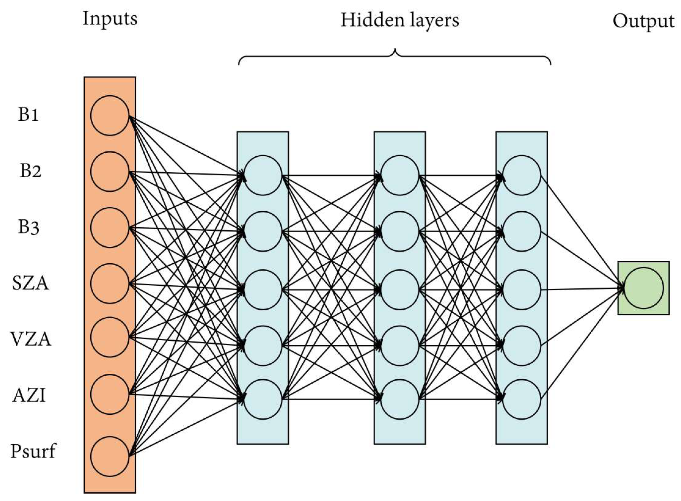
Neural Network Inversion Algorithm

Sontag [92] theoretically demonstrated that any inversion problem can be addressed using a multilayer perceptron network with two hidden layers. This approach does not require linear assumptions regarding the radiative transfer equation or the assumption of normality in random variables, making it a powerful tool for solving nonlinear problems. With the advancement of artificial intelligence technology, although training neural networks is time-consuming and demands extensive a priori knowledge, they can perform efficient numerical iterative calculations during model application to meet the real-time data processing needs. Currently, this method is used to retrieve the mean atmospheric carbon dioxide concentration in the troposphere from meteorological satellites [93,94].

The neural network inversion CO₂ algorithm estimates unknown CO₂ concentrations by creating a neural network model that relates observed remote sensing data to known CO₂ levels. This algorithm features adaptive learning and intelligent decision-making capabilities, with its core principle being the establishment of a nonlinear mapping between the observed data and CO₂ concentrations. Compared to parametric regression models, neural networks are better equipped to handle spatiotemporal variability and model complex nonlinear relationships, leading to superior prediction performance [95]. However, their application in CO₂ modeling remains limited. Additionally, due to the complex effects of clouds on thermal infrared outgoing radiation, neural networks are typically effective only for inversion under clear sky conditions.

Turquety et al. [96] developed a rapid neural network-based algorithm for IASI sensors, enabling nearly real-time inversion of CO and CH₄. Crevoisier et al. [97] utilized a neural network algorithm to invert the 5° $\times$ 5° distribution of CO₂ over the global tropical oceans using clear-sky data from IASI. They compared their 2008 inversion results with previous CONTAIL flight data, confirming consistent temporal and spatial distribution trends. Minjie Wu [98] introduced a new, fast algorithm for the radiative transfer model of the hyperspectral thermal infrared atmosphere, leveraging radial basis function (RBF) neural network techniques. This multilayer neural network, trained for specific bands, efficiently calculates radiative transfer brightness at the top of the hyperspectral thermal infrared atmosphere. Wu’s experimental results demonstrated that this algorithm not only achieves high computational accuracy but also increases processing speed by over 100 times compared to traditional radiative transfer models. Zeng et al. [99] employed a feed-forward neural network (FFNN) with a sigmoid function, using variables such as moon phase, latitude, longitude, sea surface temperature, sea surface salinity, and chlorophyll-a concentration (CHL) to model XCO₂ concentrations over the ocean. Siabi et al. [100] used a multilayer perceptron (MLP) to simulate monthly XCO₂ coverage based on data from the Orbiting Carbon Observatory-2 (OCO-2) and eight environmental variables, highlighting the application of machine learning in satellite XCO₂ retrieval. Bril et al. [101] proposed a novel retrieval algorithm for rapid XCO₂ extraction from GOSAT observation spectra, employing an empirical orthogonal function approach with GOSAT training sets and ground observations. Wu Hao et al. [102] developed a BRDF model [103] for inversion using single observations from MODIS surface two-way reflectance distribution function (BRDF) data. Their model, applied to the urban area of Beijing over five years (2011–2016), facilitates the simultaneous inversion of surface BRDF parameters and atmospheric CO₂ content.

David et al. [104] introduced an alternative method using artificial neural network (ANN) techniques to estimate XCO₂ from OCO-2 spectral measurements. The model was trained on real nadir-mode measurements collected during cloud-free conditions in even-numbered months and was subsequently evaluated using similar observations from odd-numbered months. Unlike the initial version of the model [105], which did not incorporate surface pressure as an input, this updated model integrates surface pressure data from numerical weather models and XCO₂ data from atmospheric transport simulations. Figure 14 illustrates the neural network architecture, which uses three-band spectra and observation geometry (including solar and field of view zenith angles: SZA and VZA, and relative azimuth angle: AZI) as inputs. Some versions of the model also include surface pressure (Psurf) as an additional input.

Zhao et al. [106] introduced a two-step machine learning approach for atmospheric XCO₂ retrieval using a multilayer perceptron neural network. This method, applied to satellite spectral measurements, aims to efficiently retrieve atmospheric CO₂ column densities. The approach involves creating a database of pressure-based line-by-line (LBL) CO₂ absorption coefficients sourced from the HITRAN spectral database [107,108]. A one-dimensional line-by-line forward radiation model is developed to simulate the GOSAT observational spectra, generating training data for the machine learning model. In the first step of the model, spectral deconvolution is performed to derive the atmospheric spectral optical thickness. This result is then used in the second step to extract XCO₂ based on the optical thickness. The results indicate that this method offers a promising alternative for efficient XCO₂ retrieval and that further improvements could enhance the model’s accuracy [109].

Figure 15 illustrates the schematic of the two-step machine learning model. In the first step, the input layer neurons represent the measured spectral intensities of 502 data points, denoted as $I_{C,\eta }$. Each spectral value is assigned to a neuron, producing the output $L_{C,\eta }$. In the second step, the model uses the lower resolution spectral optical thickness ${\tau }_{C,\eta }$, obtained from the first step, as input to predict XCO₂ directly after network training.

Yunfei Miao et al. [110] developed a machine-learning-based remote sensing inversion method for short-wave infrared channel CO₂ satellites. They created a training dataset incorporating satellite observation irradiance, aerosol optical thickness, and temperature. A feed-forward neural network, combined with a quantized conjugate gradient algorithm, was used to develop an inversion model for CO₂ concentrations based on GOSAT satellite spectral data. The results confirmed the effectiveness of this inversion method. Wang Biao et al. [111] integrated HITRAN database simulations with a BP neural network deep learning approach to propose a CO₂ concentration inversion algorithm. This algorithm, which can be implemented on SIM32F407, showed minimal detection errors, providing a theoretical foundation for embedded concentration inversion systems.

Neural network-based models and inversion algorithms can offer accurate and rapid processing for real-time satellite atmospheric parameter applications, with accuracy controlled within 2% [96]. However, these methods demand high spectral resolution and extensive statistical data for training and may struggle with unknown scenarios. At present, neural network algorithms are less mature and reliable compared to physical methods.

3.2.5. NLS-4DVar Data-Assimilation Algorithm

Obtaining accurate CO₂ concentrations and vertical profiles from satellite measurements remains challenging [8], with some algorithms providing reliable results only under very clear skies. This difficulty arises from the limitations in parameterization and simplification in the algorithms, such as the time-consuming burden of initial guesses for CO₂ profiles, atmospheric parameters, and their vertical distributions, as well as the simplification of calculating the weighting function matrix. Jin et al. [112] proposed a new algorithm called the Nonlinear Least Squares Four-Dimensional Variational Data-Assimilation (NLS-4DVar)-based CO₂ Retrieval Algorithm (NARA). This algorithm utilizes parameters from the LIDORT radiative transfer model and the ACOS algorithm in the forward model, optimizing state vectors to compute accurate carbon dioxide column averages, constrained by satellite measurements and prior information. The NLS-4DVar method simplifies the process by reformulating the cost function as a nonlinear least squares problem, which eliminates the need to compute the weighting function matrix and its transpose. This reduction in computational complexity is crucial for handling large data volumes in satellite retrievals while maintaining accuracy.

The NARA algorithm consists of data preparation, XCO₂ retrieval, and bias correction. The NARA algorithm flowchart is shown in Figure 16.

The NARA algorithm is effective for retrieving XCO₂ and CO₂ profiles from any GHG satellite, though it requires modifications based on satellite instrumentation. The relatively large daily standard deviation in XCO₂ retrievals, especially over oceans, results from differences in observation modes, surface properties, and varying accuracies of prior values. Land and ocean surface reflections are modeled differently—Lambertian over land and Cox-Munk with a Lambertian component over water. Factors contributing to the large standard deviation include the complex ocean surface modeling with the Cox-Munk model, variations in observation modes and satellite instrument sensitivity, and inaccuracies in prior values like initial state vectors and ensemble forecasts. Environmental variability, such as weather and surface roughness, also increases retrieval variability. Future work will focus on optimizing surface reflection models, improving observation modes, and enhancing prior value accuracy to boost the algorithm’s robustness over marine areas.

3.3. Summary

This section provides an overview of the various inversion algorithms and their accuracies applied to satellite data for deriving CO₂ column concentrations. These inversion algorithms are generally classified into two main categories: empirical statistical methods and physical methods.Empirical statistical methods can bypass the complex calculations required for radiative transfer. However, they often suffer from significant inversion errors due to factors such as sample set selection, model simplifications, and inadequate error estimation. Consequently, these methods typically cannot produce reliable global CO₂ satellite products and are usually employed to supply the a priori information needed by physical algorithms [113].

Despite advancements in remote sensing inversion algorithms both domestically and internationally, there is still a need for improvement. Enhanced algorithms and refined orthorectified radiative transfer models are required to achieve high-quality observations of CO₂ and CH₄ with improved accuracy, coverage, reliability, and computational efficiency.

4. Carbon Flux Data Assimilation and Inversion Studies

Carbon flux-assimilation inversion is a technique that integrates atmospheric carbon-assimilation models, observational data, and statistical tools to estimate the carbon dioxide absorption by ecosystems. This method enhances our understanding of carbon exchange on Earth’s surface and is crucial for global carbon-cycle research. It employs an atmospheric transport model as the forward model and continuously refines prior carbon fluxes using a Bayesian and data-assimilation-based optimization algorithm by comparing simulated and observed CO₂ concentrations. Carbon flux-assimilation inversion leverages various technical methods, effectively capturing both anthropogenic CO₂ emissions and natural variations in land-air CO₂ fluxes, making it a prominent approach in carbon-cycle research.

Building and applying an atmospheric CO₂ carbon-assimilation system involves several key aspects, including selecting assimilation algorithms, designing assimilation frameworks, processing observational data, and weighting prior fluxes. Due to the complexity and breadth of the global carbon-assimilation system, providing a comprehensive overview in a brief space is challenging. Consequently, this chapter offers an in-depth introduction to the historical development, primary research methods, notable achievements, and recent advancements in atmospheric carbon-assimilation systems.

4.1. History of the Development of the Data-Assimilation System for Atmospheric CO₂

The atmospheric CO₂ data-assimilation method belongs to the “top-down” approach for estimating surface carbon sources/sinks. It involves comparing simulated and observed atmospheric CO₂ concentrations and using optimization algorithms to adjust carbon source/sink data, thereby inferring global or regional carbon source/sink distributions. This method is an important approach for carbon source/sink estimation, providing an effective means for estimating carbon fluxes in regional and global ecosystems.

Early atmospheric carbon data-assimilation models had many issues. Due to the limited number of CO₂-observation sites, their temporal resolution was yearly, and the Transcom carbon-assimilation framework divided the world into 23 regions with coarse spatial resolution. In the case of difficulty in improving the density of ground-based atmospheric CO₂ observations, researchers began to improve and optimize the atmospheric CO₂ data-assimilation framework. Deng et al. [114] subdivided the regions and introduced a nested model based on the Transcom system, which improved the spatiotemporal resolution of carbon source and sink inversion.

In order to comprehensively understand the global carbon cycle and the spatiotemporal evolution mechanism of carbon sources and sinks, the National Oceanic and Atmospheric Administration (NOAA) of the United States developed the world’s first global carbon-tracking-assimilation system (Carbon Tracker, CT) in 2007 [115]. It assimilates global ground and aircraft CO₂ concentration observations to optimize weekly global ecosystem carbon fluxes. The system uses a nested atmospheric transport model (1° × 1° for North America and 3° × 2° for other regions) and assimilates global ground and aircraft CO₂ concentration observations to optimize weekly global ecosystem carbon fluxes. In addition, the team developed the Carbon Tracker-Lagrange carbon-assimilation system based on the Lagrangian particle dispersion model [116]. In 2005, the European Centre developed the CAMS carbon-assimilation system based on the LMDz model, using the variational assimilation method [117]. Currently, many countries and regions around the world have transplanted and improved the Carbon Tracker system, establishing localized carbon-assimilation inversion systems such as CT-Australasia, CT-Asia [118], CT-Europe [119], and CT-China [120]. However, the CT system uses the Ensemble Kalman Filter (EnKF) method. Theoretically, a single assimilation window can only assimilate observations from one time point and one type of observation data, which limits the effective utilization of rich information from multiple sources and frequencies of observational data. On the other hand, the CT system overlooks the impact of initial errors in atmospheric CO₂ concentration on the optimization results. The simulation errors in CO₂ concentration accumulate with the forward integration of the atmospheric transport model, increasing the uncertainty of the results. Additionally, mismatches between models and observational data and high computational costs present challenges. Despite these issues, modern systems like Carbon Tracker significantly enhance the accuracy of carbon flux estimates by integrating global observational data and employing higher resolution models, though the scarcity of observational data in some regions remains a concern.

Based on the Carbon Tracker system and its improved carbon-assimilation inversion systems, researchers from various countries have conducted numerous estimations of carbon sources and sinks. Ingrid et al. [121] improved the core module of the CT-Europe system and used the newly improved carbon-assimilation inversion system to estimate global carbon fluxes, revealing the distribution of carbon sinks in terrestrial and marine ecosystems. Kim et al. [122] used the Carbon Tracker system with a three-layer nested model to estimate carbon sources and sinks in the Asian region, and the results showed good performance of the Carbon Tracker system. Jiang et al. [123] and Zhang et al. [124] simulated and analyzed the spatiotemporal distribution of carbon sources/sinks in the Chinese region using the nested atmospheric CO₂ Transcom assimilation system and the Carbon Tracker assimilation system, respectively. Their results indicated that the terrestrial ecosystem in China is a large carbon sink that has been underestimated. Around 2014, the NASA team developed the CMS-Flux system based on the GEOS-Chem model for CO₂ flux estimation and attribution, using the four-dimensional variational assimilation method. Other global carbon-assimilation systems include PHILIP, AMES, and BAKER, which are based on the GEOS-Chem model and PCTM transport model, respectively. All of these model systems participated in the OCO-2 MIP model intercomparison project, which provided multi-model inversion results of CO₂ fluxes in land systems of various countries from 2015 to 2020.

China’s advancements in carbon-assimilation inversion research have been noteworthy despite a late start. In 2015, the GCAS (Global Carbon-Assimilation System) was developed, incorporating an atmospheric transport model, a terrestrial ecosystem process model, and a land–atmosphere-assimilation system using the four-dimensional variational assimilation method [124]. Although this system laid a solid foundation, it initially struggled with integrating diverse observational data effectively. The creation of the China Carbon-Tracking-Assimilation System (CT-China) by adapting the CarbonTracker system provided a robust framework but did not fully address previous limitations. In 2016, Nanjing University developed GCAS-v2, enhancing spatial resolution to 1° $\times$ 2.5° and 4D sliding sampling [125], though spatial resolution issues persisted. Regionally, the CFI-CMAQ system by Nanjing University and the Institute of Atmospheric Physics employed advanced ensemble methods for CO₂ data assimilation but faced scaling challenges [126]. Lu Lijiang’s Tracers Tracker combined the ensemble four-dimensional variational method with the CMAQ model for high-resolution regional analysis but lacked integration with ecological models, limiting its optimization of carbon fluxes from photosynthesis and respiration. Despite these advancements, integrating ecological models and optimizing data assimilation across various scales remains a challenge.

All of the above-mentioned global carbon-assimilation systems optimize the CO₂ flux between the land surface and the atmosphere, assuming that the error in anthropogenic carbon flux can be ignored, in order to obtain the net carbon flux between the terrestrial ecosystem and the atmosphere. The atmospheric carbon-assimilation inversion system is still constrained by observational data, and the observational data it relies on are still global ground-based observational data, resulting in large uncertainties in the simulation results of carbon sources/sinks.

4.2. Data-Assimilation Algorithms

Assimilation systems typically include process models, observational data, assimilation algorithms (or schemes), and observation operators. Data-assimilation algorithms are central to these systems, serving as the crucial link between observational data and models. This process involves dynamically integrating new observational information—characterized by various types, spatiotemporal scales, and varying accuracy—into numerical models. It takes into account data distribution, background field errors, and observation errors to provide the most accurate estimation of model parameters and state variables [127].

From an algorithmic perspective, data-assimilation methods fall into two primary categories: sequential assimilation algorithms and variational assimilation algorithms [128]. Modern techniques are further classified into variational methods based on optimal control theory and ensemble Kalman filtering rooted in estimation theory. Most contemporary assimilation methods can be expressed by the following formula:

$$x^{opt}=x_b+W(y^{obs}-y)$$

(12)

where $x^{opt}$ is the optimal value; $x_b$ is the background value; $y^{obs}$ is the observed value; y is the simulated value; and W is the difference between the different assimilation methods, which yield different a posteriori weights [129]. Due to the limitations of instruments and observation conditions, there are some differences between the observed data and the “real data”, i.e., the observation error, which can be expressed as follows:

$$\widehat{x}=x_b+{\epsilon }_b$$

(13)

$$y^{obs}=H\left(x_0\right)+{\epsilon }^{obs}$$

(14)

where $\widehat{x}$ is the truth value; $x_b$ is the background field; ${\epsilon }_b$ is the error between the background field and the truth value, and the background error covariance matrix is denoted by B; $y^{obs}$ is the observed non-conventional data matrix; $x_0$ is the variable to be solved by the model; H is the observation model operator; the observation error ${\epsilon }^{obs}$, denoted as matrix R, includes the discrepancy between the observed data and the true value, the error caused by the observation operator, and the representative error generated when mapping the state variables to the observation space. These two types of errors control the operation of the assimilation process and ultimately yield the analysis error. The purpose of data assimilation is to minimize the final analysis error.

This section first reviews the data-assimilation methods used in the early stage, compares the improvements of these assimilation methods and explains modern assimilation algorithms such as three-dimensional and four-dimensional variational assimilation, Kalman filtering, ensemble Kalman filtering, and neural network algorithms. Finally, it analyzes and comments on these assimilation algorithms.

4.2.1. Overview of Assimilation Data

In 1949, Panofsky [130] introduced the polynomial interpolation method, primarily based on least squares fitting of regional polynomials that include observation points. In 1955, Bergthorsson et al. [131] presented the background field analysis method, arguing that initial values should be incorporated in objective analysis to address the problem of insufficient observations. Building on background field analysis, two variations of interpolation methods were developed: the successive correction method (SCM) and the optimal interpolation method (OI). During the 1980s and 1990s, variational assimilation methods, such as three-dimensional variational assimilation (3D-VAR) and four-dimensional variational assimilation (4D-VAR), effectively tackled the nonlinearity issues in data assimilation [132]. Wang et al. [133] categorized these approaches into three stages: simple analysis methods, statistical or OI methods, and variational analysis.

After the 1990s, sequential assimilation algorithms, notably the Kalman filter (KF) and its derivatives, became predominant. Recently, various particle filter (PF) algorithms derived from the ensemble approach have rapidly evolved and gained widespread use. Traditional KF algorithms are mainly suited for linear system models, while many sequential assimilation algorithms have been adapted for complex, nonlinear models, such as the extended Kalman filter (EKF) [134], unscented Kalman filter (UKF) [135], and ensemble Kalman filter (EnKF) [136]. Although the ensemble Kalman filter offers advantages over earlier algorithms, it faces challenges like rank-deficient inverses in the gain matrix and filter divergence. To address these issues, several ensemble Kalman filter-based algorithms have been improved and optimized, including the ensemble transform Kalman filter (ETKF) [137], ensemble square root filter (EnSRF) [138], ensemble adjustment Kalman filter (EAKF) [139], local ensemble Kalman filter (LEKF) [140], and ensemble steady-state Kalman filter (EnSSKF) [141].

Additionally, the particle filter, a novel sequential assimilation algorithm based on Monte Carlo simulation and Bayesian sampling, is particularly effective for complex nonlinear and non-Gaussian system models. With a sufficient number of particles, it can achieve near-optimal accuracy and deliver robust results, demonstrating considerable potential for various applications. The field of data assimilation is also evolving with the integration of artificial intelligence technologies, including genetic algorithms, neural networks, and simulated annealing, leading to the development of modern intelligent assimilation algorithms.

4.2.2. Data-Assimilation Algorithms

This part introduces 3D-VAR, 4D-VAR, Kalman Filter (KF), EnKF algorithm, and Neural Network algorithm.

3D-Var & 4D-Var

Three-dimensional variational analysis (3D-Var) compares the observed fields at different time steps with the analysis fields obtained by forward calculation from the initial fields. By defining a function for the initial fields and using a certain descent algorithm, the gradient function of the corresponding initial fields is solved to minimize the function and obtain the optimal initial fields. Compared to optimal interpolation, three-dimensional variational analysis has a larger amount of data analysis and can perform global analysis, avoiding local discontinuity issues.

Three-dimensional variational analysis is based on the theoretical methods of Bayesian filtering and maximum likelihood estimation. The objective function of 3D-Var [142] is as follows:

$$J\left(x_0\right)={\displaystyle \frac{1}{2}}{(x_0-x_b)}^T{B}^{-1}(x_0-x_b)+{\displaystyle \frac{1}{2}}{[H\left(x_0\right)-y^{obs}]}^T{R}^{-1}[H\left(x_0\right)-y^{obs}]$$

(15)

where $x_0$ represents the variable to be solved for. The formula can also be interpreted as assuming that the background field and error covariance are known, and ultimately the goal is to minimize the total analysis error covariance. The purpose of solving the cost function is to find an optimal initial field $x_0$ that minimizes the cost function. The solution of the cost function is mainly achieved through the gradient function, which is iteratively solved using the following equation:

$$\nabla J=\nabla J_b+\nabla J_0=B^{-1}(x_0-x_b)+H^T{R}^{-1}[H\left(x_0\right)-y^{obs}]$$

(16)

where H represents the tangent linear mode of the observation operator; $H^T$ is the concomitant operator of this tangent linear mode. The number of iterations can be set artificially or stopped by setting $\nabla J$ a decreasing limit.

Three-dimensional variational assimilation (3D-Var) utilizes observations from specific time points, whereas four-dimensional variational assimilation (4D-Var) extends this by incorporating a forecast operator, thus integrating observations over time. Talagrand and Coutier [143] significantly advanced 4D-Var by introducing the adjoint model, simplifying its solution and fostering its development. Unlike 3D-Var, the cost function in 4D-Var assimilation includes both the observation operator and the forecast model, thus extending the analysis across the temporal dimension. However, this temporal extension increases the computational cost and memory usage of 4D-Var and complicates the solution of the tangent linear adjoint model, which remains a challenging task [144].

The objective function of 4D-Var is:

$$\begin{array}{c}\hfill J\left(x_0\right)={\displaystyle \frac{1}{2}}{(x_0-x_0^b)}^T{B}^{-1}(x_0-x_0^b)+{\displaystyle \frac{1}{2}}{\displaystyle \sum _{n=0}^N}\{H_n\left\{M_n[\cdots M_0\left(x_0\right)]\right\}-\\ \hfill y_n^{\mathit{obs}}{\}}^T{R}_n^{-1}\left\{H_n\left\{M_n[\cdots M_0\left(x_0\right)]\right\}-y_n^{\mathit{obs}}\right\}\end{array}$$

(17)

where $x_0$ is the state at the initial moment; $x_0^b$ is the initial background field; $y_n^{obs}$ is the observation at the nth moment; $M(t_0,t_i)\left(x_0\right)$ is the state quantity predicted by the nonlinear model at the $t_i$ moment; $H_i$ is the observation operator that maps the state variables to the observation space at the $t_i$ moment; B is the background error covariance; R is the observation error covariance at the $t_i$ moment [145].

4D-Var variational assimilation is a nonlinear optimization problem under constraint conditions. The solution to the four-dimensional variational assimilation problem adopts a similar algorithm to the three-dimensional variational assimilation, using the adjoint method and the optimal control theory of partial differential equations to solve it.

The gradient of the objective function in 4D-Var is obtained as follows:

$$\begin{array}{c}\hfill {\displaystyle \frac{\partial J\left[x\left(t_0\right)\right]}{\partial x}}=B^{-1}[x\left(t_0\right)-x^b\left(t_0\right)]+H_0^T{d}_0+M_0^T[H_1^T{d}_1+\\ \hfill M_1^T(H_2^T{d}_2+\cdots +M_n^T\left(H_n^T{d}_n\right)\cdots ]\end{array}$$

(18)

In the equation, $d_n=R_n^{-1}[H_n\left(x_n\right)-y_n^{obs}]$. During the minimization process, the adjoint matrix is used to search for the gradient information corresponding to the initial state in order to reduce the value of the objective function. This involves forward integration of the forecast model once and backward integration of the adjoint equation to the initial time to adjust the gradient of the cost function. The adjusted initial field is then used in the forward model. This process is repeated in a loop until the convergence condition is met.

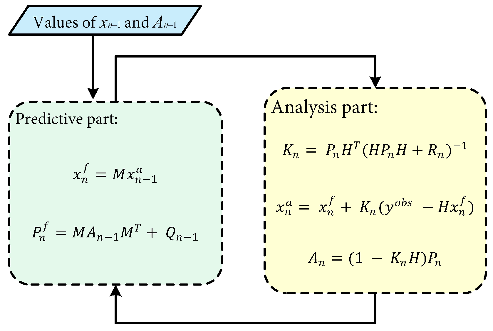
Kalman Filter Algorithm (KF)

The classic Kalman filter assimilation algorithm is an optimal recursive data processing method. It estimates the state variables by utilizing the statistical characteristics of the observations, as well as the errors between the model and the observations. The basic idea is as follows: first, make a forecast of the state variables, then introduce the observation data, reanalyze the state variables based on the observation data, and then make another forecast. This completes the cycle of forecast-analysis-forecast [146].

The Kalman filter consists of two parts: prediction and analysis, with a total of 5 equations, expressed as follows [147].

Prediction part:

$$x_n^f=M{x}_{n-1}^a$$

(19)

$$P_n^f=M{A}_{n-1}{M}^T+Q_{n-1}$$

(20)

The first equation is the prediction of the state variable, $x_n^f$ denotes the prediction operator M forward integrating to obtain the predicted value of the state quantity at the n moment; the second equation is the prediction of the prediction error covariance $P_n^f$, which can be considered to be composed of two parts, one of which is the part of the initial value as well as the part of the error caused by the evolution of its model, and the other part of which is the model’s prediction error at the nth moment $Q_{n-1}$, which is caused by the model itself, such as the driving data and the error of boundary conditions, the error of model parameters, etc. [148], $A_{n-1}$ is the analyzed error of the previous moment.

Analysis part:

$$K_n=P_n{H}^T{(H{P}_n{H}^T+R_n)}^{-1}$$

(21)

$$x_n^a=x_n^f+K_n(y^{obs}-H{x}_n^f)$$

(22)

$$A_n=(1-K_{n}H)P_n$$

(23)

where $K_n$ denotes the Kalman gain at the n moment, H is the observation operator used to project the state variables into the observation space, and $R_n$ is the observation error covariance; a posteriori adjustments to the state quantities can be made using the second equation, which is the same as the OI and the update formula in the variational assimilation and is obtained by multiplying the predicted value (or the background value) plus an increase in the observed value by a certain weight, K; the third equation concludes with an analytical error covariance that can be used to predict the prediction error covariance at the next moment.

The whole process of Kalman filtering is shown in Figure 17.

Ensemble Kalman Filter Algorithm (EnKF)

The ensemble Kalman filter algorithm is a method that uses a limited ensemble and is based on the Monte Carlo algorithm to estimate the error covariance [136,149]. It generates a certain number of ensembles by adding perturbations to the background field and observation values and obtains the corresponding analysis values. Then, based on the differences in these values, it statistically calculates the error covariance matrix. The biggest advantage of the ensemble Kalman filter algorithm is that it does not require the development of tangent linear and adjoint models, and it can explicitly provide initial perturbations for ensemble forecasts. For the k ensembles X at time step $n-1$, the predicted state variables are as follows:

$$x_{k,n}^f=M{x}_{k,n-1}^a+{\epsilon }_{k,n-1}$$

(24)

where M is the prediction model; ${\epsilon }_{k,n-1}$ is the corresponding error term. By using these randomly simulated sets, the covariance of the sample error can be estimated.

$$P_n^f={\displaystyle \frac{1}{K-1}}{\sum }_{i=1}^K[x_{k,n}^f-\overline{x_n^f}]{[x_{k,n}^f-\overline{x_n^f}]}^T$$

(25)

$$\overline{x_n^f}={\displaystyle \frac{1}{k}}{\sum }_{i=1}^k{x}_{k,n}^f$$

(26)

where $x_{k,n}^f$ is the forecast value of the k ensemble at the nth moment. Theoretically, as the number of ensembles N rises, the Monte Carlo sampling error decreases proportionally to $1/\sqrt{N}$ [147], but the rise in the number of ensembles brings with it a greater amount of computation and memory. The state update equation can also be obtained for the set Kalman:

$$x_{k,n}^a=x_{k,n}^f+P_n^f{H}^T{(H{P}_n^f{H}^T+R_{n-1})}^T(y_{k,n}^{obs}-H{x}_{k,n}^f)$$

(27)

$$P_n^f{H}^T={\displaystyle \frac{1}{K-1}}{\sum }_{i=1}^K[x_{k,n}^f-\overline{x_k^f}][H(x_{k,n}^f)-\overline{H(x_k^f}){]}^T$$

(28)

$$R_{n-1}={\displaystyle \frac{1}{k-1}}{\sum }_{i=1}^N[y_{k,n-1}^{obs}-\overline{x_k^f}][H(x_{k,n}^f)-\overline{H(x_k^f}){]}^T$$

(29)

where M and H are the model operator and observation operator respectively; R is the observation error covariance, and $y_{k,n-1}^{obs}$ is also the observed value of the k ensemble at the nth moment; $x_{k,n}^a$ is the value obtained from the k ensemble corrected at the nth moment. The analyzed error covariance can be calculated as follows:

$$A_n={\displaystyle \frac{1}{K-1}}{\sum }_{i=1}^K[x_{k,n}^a-\overline{x_k^a}]{[x_{k,n}^a-\overline{x_k^a}]}^T$$

(30)

The size of the set ranges from dozens to hundreds depending on the situation. As the number of sets increases, the estimation accuracy is expected to be higher. However, the computational complexity also increases. If the number of sets is too small, the average value cannot truly represent the objective state. Therefore, further research is needed to determine the most appropriate number of sets to choose.

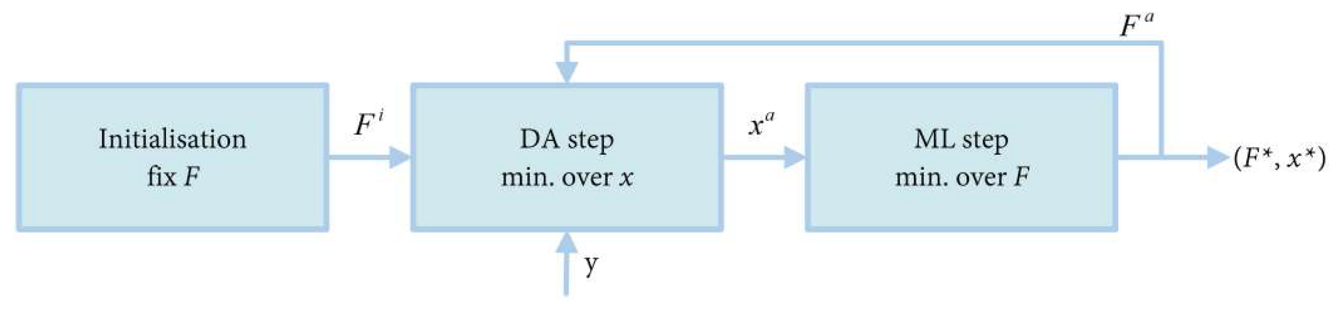
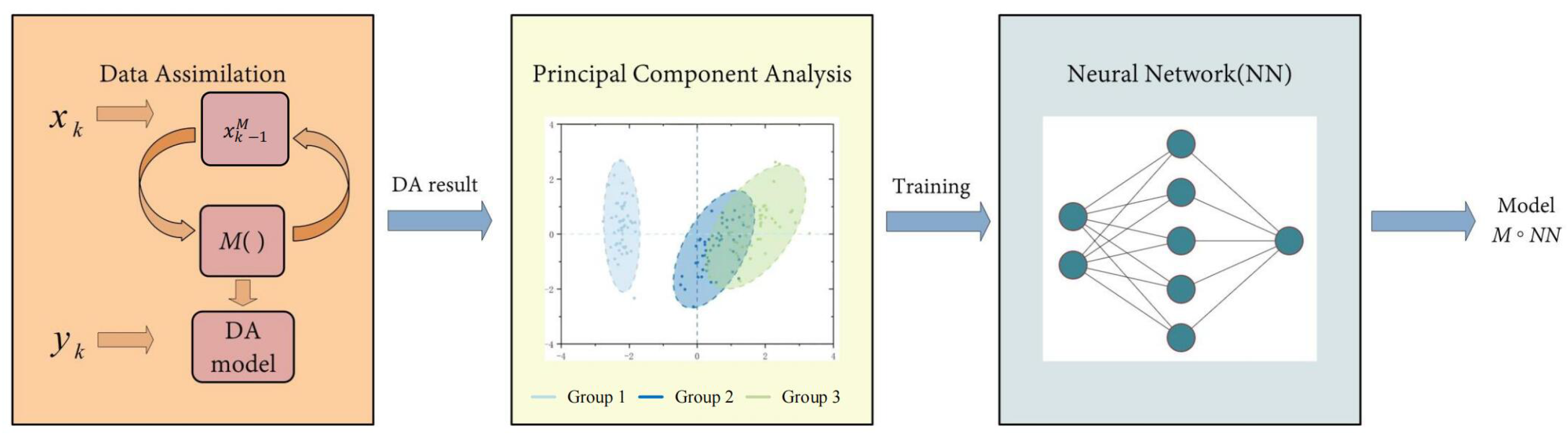
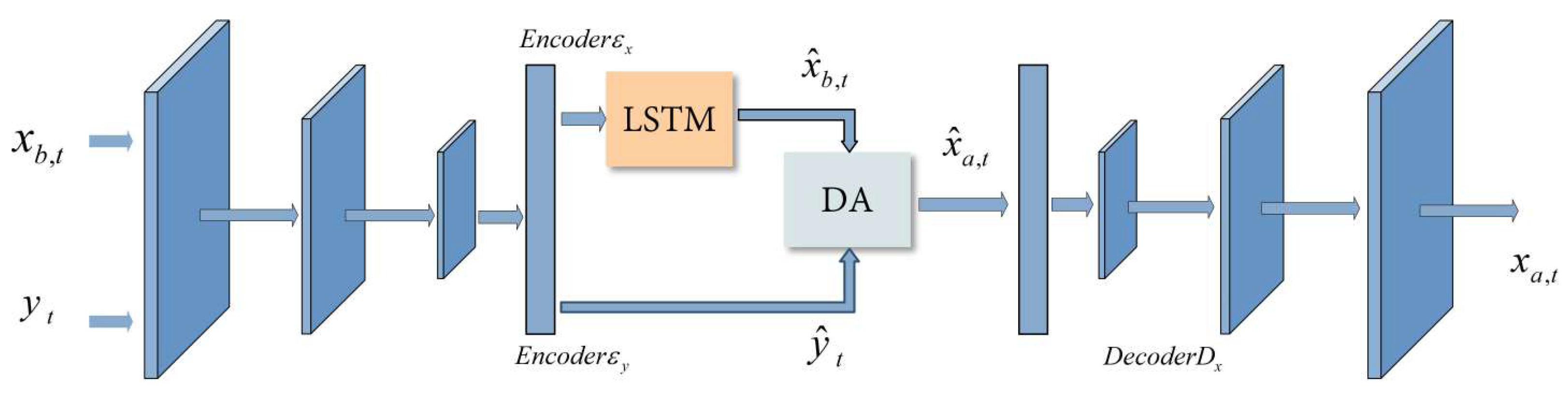
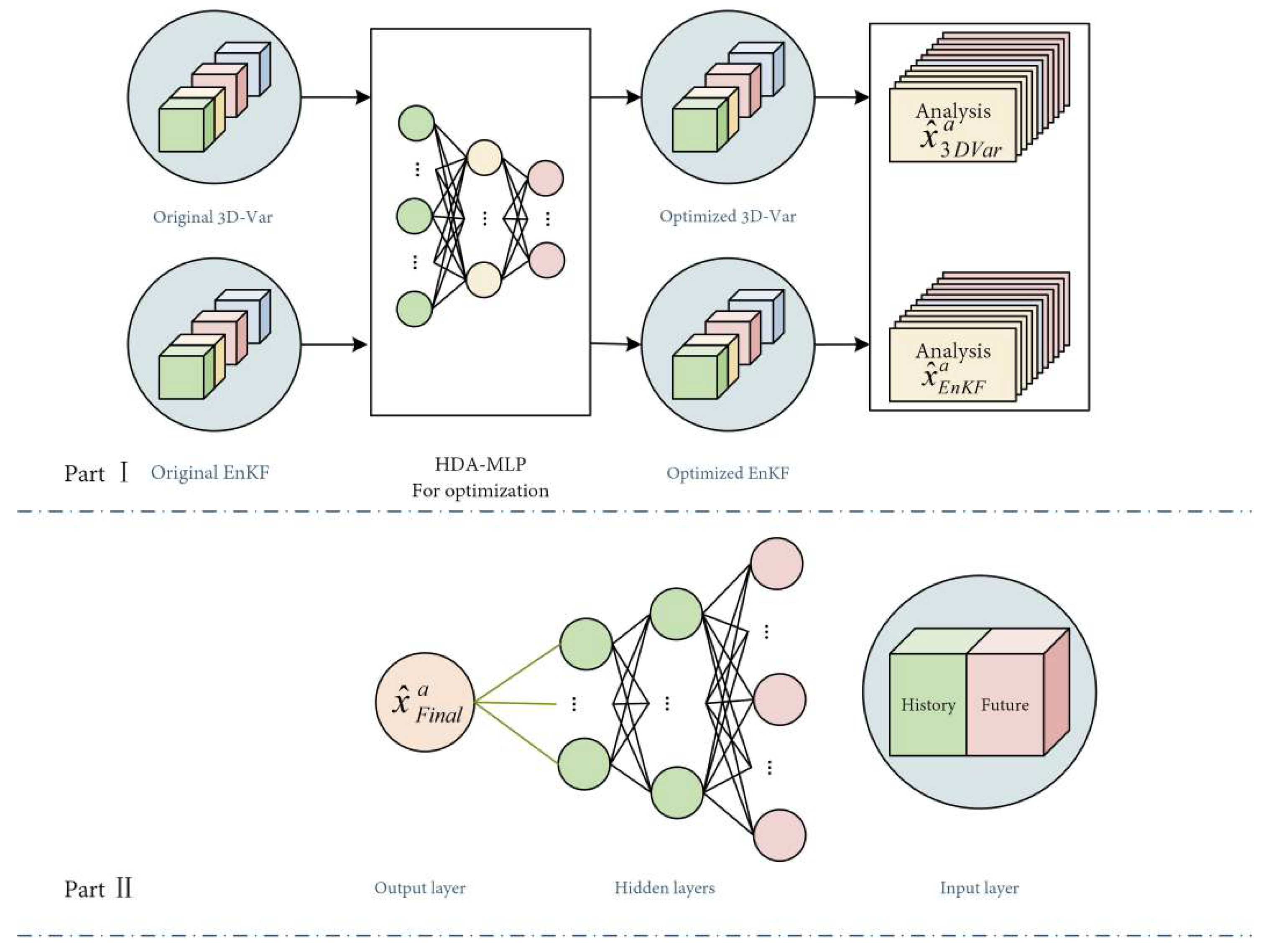
Machine Learning (ML) Algorithms

The advent of remote sensing satellites, the increase in observational data, and the rising demand for accuracy necessitate more sophisticated variational methods and Kalman filter models to meet application needs and mitigate implementation challenges. However, these methods continue to grapple with issues related to model errors, parameter estimation, and error covariance specification [150]. Recently, machine learning (ML) has shown promise in approximating nonlinear systems and extracting meaningful insights from high-dimensional data [151,152]. ML algorithms can complement or even replace traditional methods by addressing their assumptions and limitations, correcting model errors, and facilitating real-time improvements and adjustments during data assimilation and prediction.

Typically, model correction methods involve using statistical models, such as neural networks, to adjust knowledge-based physical models. One straightforward approach is to apply a correction to each model. Brajard et al. [153] proposed an offline learning method that alternates between data assimilation (DA) and ML to learn system states and observations in sparse and noisy environments. This method, which minimizes a defined loss function through coordinate descent [154], is illustrated in Figure 18. Additionally, Bocquet et al. [155,156,157] developed an online learning method that replaces offline learning, utilizing enhanced state DA techniques to estimate system states and statistical correction parameters.

Due to the complexity of system models, online parameter estimation for high-dimensional dynamical systems has long been a challenge [158]. For handling high-dimensional big data, reduced-order modeling and low-dimensional surrogate models generated by machine learning algorithms have been increasingly applied to enhance algorithm efficiency. Traditionally, dimension reduction methods included Principal Component Analysis (PCA) and Empirical Orthogonal Function (EOF) techniques. Buizza et al. [159] proposed a deep learning (DL) model that integrates Kalman filter-based reduced-order modeling, neural networks, and data assimilation, as shown in Figure 19. This model combines the efficiency of reduced-order modeling (ROM), the accuracy of data assimilation (DA), and the speed of deep learning. It effectively addresses issues such as dimensionality constraints, noisy data, and low-quality data, with PCA enabling DA to be conducted in a reduced-dimensional space.

Chen et al. [160] introduced Generalized Latent Assimilation (GLA), a system that integrates a reduced-order surrogate model using Autoencoder (AE) and Long Short-Term Memory (LSTM) techniques with advanced data-assimilation methods. This system adjusts model parameters in real-time by incorporating observational data. Additionally, it employs a local smoothing surrogate function to connect the spatial representation of encoded system variables with current observations, facilitating variational data assimilation while reducing computational costs. The flowchart for Generalized Latent Assimilation is depicted in Figure 20.

Error covariance matrix modeling is a crucial component in data-assimilation algorithms, as it significantly impacts prediction accuracy. Estimating these covariances typically relies on empirical assumptions and physical constraints, which can be imprecise and computationally demanding, particularly for high-dimensional systems.

Cheng et al. [161] developed and tested an innovative data-driven approach using Long Short-Term Memory Recurrent Neural Networks (LSTM) to enhance the accuracy and efficiency of covariance specification for dynamic data-assimilation problems. During training, synthetically generated observation sequences are used as inputs to the LSTM. A key advantage of this data-driven approach is its ability to handle both non-parametric and parametric covariance models.

Lilan Huang et al. [162] introduced a new data-driven method called HDA-MLP to address data-assimilation challenges, as illustrated in Figure 21. This method involved formal optimization of individual data-assimilation techniques (3D-Var and EnKF) using Multi-Layer Perceptrons (MLP), while another neural network model implicitly updated the background error covariance matrix. By leveraging short-term predictions to correct current assimilation results, this approach reduced dependence on traditional data-assimilation methods. The results demonstrated improved robustness and a better capability to capture variations in state variables, significantly enhancing both the quality of the analysis and computational efficiency.

Recent research has increasingly employed machine learning (ML) techniques to develop end-to-end learning solutions for entire data-assimilation (DA) systems, mapping observed data directly to target state sequences or model parameters. Zhu et al. [163] introduced a framework that integrates neural networks (NN) with physical models via a data-assimilation algorithm to enhance model error correction and prediction accuracy, as depicted in Figure 22. The effectiveness of this framework was demonstrated through various case studies and sensitivity analyses. The figure illustrates the overall process of the Deep Data-Assimilation (DDA) model. The paper introduces the network $G_{\omega }$, with the training objective of this network being:

$$x_k=G_{\omega }\left(F\left(x_{k-1}\right)\right)$$

(31)

The article takes the values of $F\left(x_{k-1}^{DA}\right)$ and $x_k^{DA}$ as inputs and outputs of the network $G_{\omega }$ and then uses the results of the DA $\left\{(x_{k-1}^{DA},x_k^{DA})\right\}$ to train $G_{\omega }$, which is updated by the observations and the gradient loss function on its parameters.

4.2.3. Summary of Data-Assimilation Algorithms

In the field of traditional data assimilation, each method has its strengths and limitations, depending on specific applications and resources. The Kalman Filter (KF) optimizes state estimates based on linear models and Gaussian noise assumptions but struggles with nonlinearity and non-Gaussian scenarios. The Ensemble Kalman Filter (EnKF) captures nonlinearity and broader uncertainties using multiple samples, though its performance is influenced by sample size. The Particle Filter (PF) addresses complex nonlinearity and non-Gaussian issues through weighted particles, albeit with high computational costs. Variational Methods optimize a cost function to integrate observations and model predictions, effectively managing uncertainty but requiring accurate error covariances and significant computational resources.

Emerging Machine Learning Methods tackle uncertainty by learning complex patterns from data, though their efficacy depends on data quality and model training. While 4D-VAR and the ensemble Kalman filter series are well-established and widely used, intelligent assimilation algorithms, including particle filters, Bayesian methods, and neural networks, represent promising directions for future development. The choice of assimilation algorithms and models in practical research largely depends on the specific characteristics of the problem (such as model structure, observation data type, and error manifestations) and available computational resources. Researchers may opt for a single suitable method or combine various methods to leverage their strengths and mitigate their weaknesses.

4.3. Framework and Techniques for Assimilation of Atmospheric CO₂

The atmospheric CO₂-assimilation system is a cutting-edge simulation tool for analyzing carbon sources and sinks in terrestrial ecosystems on global or regional scales. It leverages prior carbon flux data from sources such as land, oceans, biomass burning, and fossil fuel emissions. The system employs an atmospheric transport model as a “forward” model and uses CO₂ concentration data as observational input. By integrating Bayesian theory with iterative solving, the system determines the optimal CO₂ flux values and ultimately simulates the spatiotemporal variations of carbon sources, sinks, and concentrations. As illustrated in Figure 23, the framework of the CO₂-assimilation system includes prior flux data, the atmospheric transport model, CO₂ concentration data, and assimilation algorithms.

4.3.1. Prior Flux

Prior flux is divided into four parts: ocean carbon flux, fossil fuel carbon-emission inventory, ecosystem carbon flux, and fire carbon-emission data. Due to the large differences in the absolute values of prior flux in different regions, it is generally not directly assimilated as a system state variable. Instead, assimilation is performed by adding a difference or multiplying by a scaling factor to the prior flux. This adjusted flux is then used as the posterior flux. The difference or scaling factor, being dimensionless, can be better used as a system state variable for statistical calculations in the carbon-assimilation system.

4.3.2. Atmospheric Transport Model

The atmospheric transport model serves as the “forward” model in the atmospheric CO₂-assimilation system, connecting atmospheric CO₂ concentrations and land surface fluxes. It simulates the distribution of atmospheric CO₂ concentrations by using land surface carbon fluxes and meteorological driving data as inputs. The model utilizes global atmospheric chemical transport models to simulate atmospheric CO₂ and compare it with observational data. This research helps understand the spatiotemporal variations of CO₂ in different regions and reveals the changes in carbon emissions and land ecosystem carbon sources and sinks in different regions globally. It is an essential component of the CO₂-assimilation system.

The atmospheric chemical transport model can be divided into mesoscale atmospheric chemical transport models and global atmospheric chemical transport models. Mesoscale atmospheric chemical transport models are commonly used to simulate the distribution of atmospheric CO₂ concentrations over a short period in a specific region. Compared to global atmospheric chemical transport models, they have higher resolution and often include nested regional models with resolutions ranging from a few kilometers to tens of kilometers. Global atmospheric chemical transport models, on the other hand, are used to simulate the distribution of atmospheric CO₂ concentrations over a longer period globally, with lower resolutions generally between 1° and 3°. Some commonly used mesoscale atmospheric chemical transport models for simulating regional atmospheric CO₂ concentrations include WRF-Ghem [164], CMAQ [165], CHIMERE [166], and REMO [167]. For simulating global atmospheric CO₂ concentrations, commonly used global atmospheric chemical transport models include GEOS-Chem [168], MOZART [169], TM [170], and LMDZ [171]. Unlike observations, atmospheric transport models can provide globally comprehensive coverage of atmospheric CO₂ concentrations with higher spatiotemporal resolutions.

However, due to the resolution of atmospheric chemical transport models and the fact that the values are averaged over a certain period and space, combined with the uncertainties in land surface carbon fluxes and the “chaotic” nature of the atmospheric system, long-term predictions of atmospheric CO₂ are challenging, and the uncertainties cannot be eliminated regardless of how accurately the physical and chemical processes of CO₂ transport are simulated by the models.

4.3.3. Satellite CO₂ Column Concentration Data-Assimilation Process

Data-assimilation techniques for atmospheric CO₂ aim to determine the optimal CO₂ flux by minimizing the difference between simulated and observed concentrations. Different assimilation methods use distinct cost functions. The assimilation process is divided into two parts: the forecast process of CO₂ flux (state forecast) and the analysis process (state analysis). The state forecast step calculates the current state variable (CO₂ flux) and estimates the error covariance to create a prior estimate for the next time step. Typically, a simple forecast model, such as the identity matrix I, is used for this. The state analysis step combines the prior estimate with new measurement data to produce an improved posterior estimate. The CO₂ flux from the forecast process serves as input for simulating current CO₂ concentrations using atmospheric transport models (e.g., TM5, GEOS-Chem). The simulated CO₂ concentrations are then compared with observed concentrations to refine the CO₂ flux and optimize carbon sources and sinks.

The satellite column concentration-assimilation-cycle integrates observations, atmospheric transport models, state forecasts, and state analysis. Unlike other data-assimilation processes, it incorporates state variables across multiple time steps within the same carbon-assimilation cycle (with a time step of one week). This approach accounts for the time lag between CO₂ flux and concentration, as the observed CO₂ concentration at any given time reflects the accumulation of CO₂ flux transport and diffusion from previous periods. This lag issue is described mathematically as a “lag window“ in the assimilation system. The entire assimilation process includes several cycles, with each cycle’s duration determined by the assimilation window. For clarity, the “lag window“ is set to 5 weeks. Figure 24 illustrates the assimilation-cycle process, where the state variable (CO₂ flux) is denoted as $x_i$ (0,1,2,3,4). The numbers in parentheses (0,1,2,3,4) indicate the number of times the state variable (CO₂ flux) has been assimilated in previous cycles, and the subscript i represents the set of state variables (CO₂ flux). The light blue box shows the background field (forecast field) of the state variable, with data representing the background state vectors. The blue area denotes the assimilation-cycle process, while the light green box represents the analysis field of the state variable, with data as the analysis state vectors.

The complete assimilation inversion CO₂-cycle process is described as follows:

(1)

In the first analysis cycle, the background state vector is updated using observational data. At time t, the driving data $x_i$(0, l, ⋯, 4) within the light blue box is used to drive the atmospheric transport model to simulate the CO₂ concentration values from ${\mathrm{CO}}_{2i}(x,y,z,t+1)$ to ${\mathrm{CO}}_{2i}(x,y,z,t+5)$ for a period of 5 weeks. The simulated concentrations are sampled based on the temporal, spatial, and elevation information of the concentration observations $y\left(t\right)$∼$y(t+5)$ to prepare for assimilation.

(2)

The assimilation process is performed on the state variables (average and deviation of CO₂ flux) $x_i$(0, l, ⋯, 4) at time t, according to the formula, to obtain the analyzed values of the state variables (CO₂ flux) within the green box for the assimilation period of 5 weeks.

(3)

The $x_i$(4) will not proceed to the next cycle at time $t+1$. The optimized state vector $x_i$(4) is used as the driving data to simulate the optimized ${\mathrm{CO}}_{2i}(x,y,z,t+1)$ concentration by the assimilation inversion module and the atmospheric transport model.

(4)

The analyzed field $x_i$(0, 1, 2, 3) at time t becomes the background field for the next cycle at time $t+1$. A new state variable $x_i$(0) and new observation data $y(t+6)$ enter the cycle to start a new assimilation process. Afterward, in each analysis cycle, the analysis state vector from the previous cycle is used as the background state vector for the current cycle.

4.4. Application of Carbon Flux Estimation Based on Assimilation Schemes

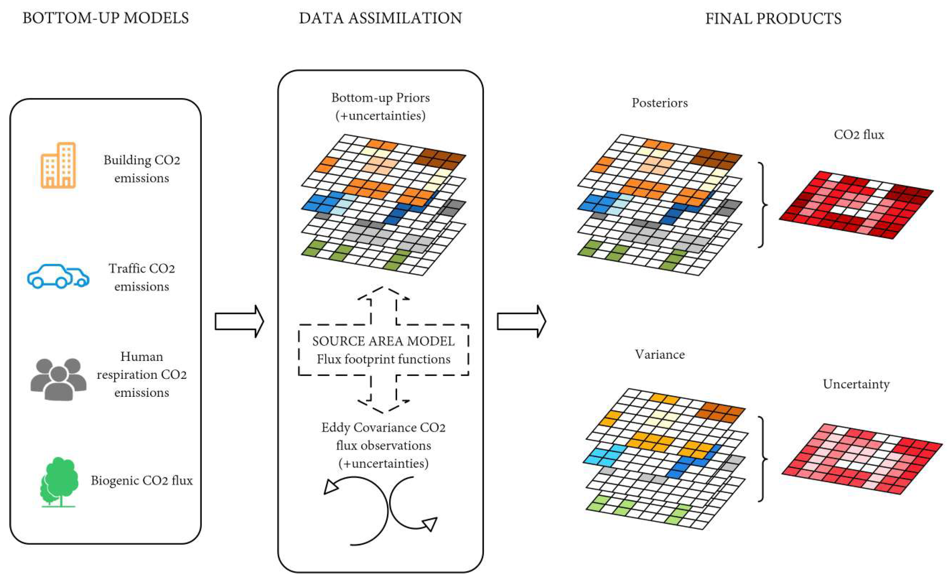
4.4.1. Optimising CO₂ Emissions in Urban Areas

Accurate monitoring of urban CO₂ emissions is essential for guiding sustainable urban development. Currently, CO₂-emission inventories are compiled using a bottom-up (BU) approach, which offers more precise prior fluxes for inverse assimilation and helps reduce prior flux uncertainties. Ground-based flux-observation networks can validate the “top-down” models and enhance inversion models [172]. However, this approach has notable limitations. Yang et al. [173] used X-STILT to analyze urban XCO₂ enhancements in five Middle Eastern cities and found that the simulation results were not sensitive to different spatial emission patterns in the bottom-up inventory, which hinders understanding of spatial and temporal emission variations. While data-assimilation (DA) techniques have been applied to urban environments [174,175,176], combining transport models with atmospheric observations to refine urban emissions, challenges remain. Urban emission studies often aim to validate bottom-up CO₂ inventories by constraining fossil fuel fluxes but frequently overlook fundamental emission processes causing discrepancies between observed and simulated concentrations. To address this, higher-resolution prior emissions are needed to capture significant spatiotemporal variations.

Super et al. [177] developed the CarbonTracker Data-Assimilation Shell (CTDAS), a city-scale DA system designed to quantify CO₂ emissions from various urban sectors. This system uses a dynamic fossil fuel-emission model with optimized parameters and the Weather Research and Forecasting-Stochastic Time-Inverted Lagrangian Transport (WRF-STILT) model to represent non-point source emissions. It also estimates model parameter uncertainties, providing insights into spatiotemporal uncertainty and error correlations among emission sources. Stagakis et al. [178] introduced a new method within the Bayesian inversion framework, combining direct CO₂ flux observations from urban eddy covariance (EC) towers with detailed data from an advanced urban BU surface flux model to refine urban emission estimates. This approach yields optimized gridded CO₂ flux information for various surface flux components—such as building heating, commercial/industrial activities, traffic, human respiration, and biotic net exchange—at a 20-m resolution and weekly time step. Figure 25 illustrates the BU model inputs as detailed by Stagakis et al. [179].

The results indicate that urban EC observations can be sustainably used to improve high-resolution BU surface CO₂ flux model estimates and provide realistic seasonal variations for each flux component. However, the current approach needs further expansion of the model domain and should be combined with atmospheric inversion methods and tall tower EC to extend the model domain to city-wide emissions and establish an observation-based comprehensive monitoring system to address potential surface flux processes at different scales.

4.4.2. Assimilation of High-Resolution Carbon Fluxes Based on Satellite Observations

In recent years, the increasing volume of CO₂-observation data has highlighted a significant challenge: the computational cost of traditional atmospheric inversion methods for CO₂ column concentration (XCO₂) products from satellite observations is prohibitively high. This makes it difficult to assimilate large datasets for high-resolution carbon flux optimization.

The global carbon-assimilation system offers a promising solution to this problem. By employing data-assimilation techniques, it helps mitigate the discrepancies between carbon flux predictions from land surface models and atmospheric CO₂ concentration measurements. This approach reduces uncertainties in land surface models and enhances carbon flux estimates by integrating observed carbon-related data [180]. For instance, European scientists have developed the Global Carbon Data-Assimilation System (CCDAS). This system assimilates a variety of data sources, including satellite and ground-based atmospheric CO₂ concentrations, site flux data, remote sensing land surface parameters, and more, to optimize ecosystem model parameters and carbon flux estimates. This process improves the accuracy of regional and global carbon source and sink estimations and lays the groundwork for developing high-resolution global carbon-assimilation systems. However, CCDAS faces challenges due to its substantial computational demands. As a result, it operates with relatively low spatial resolution and has limited capacity for incorporating ground-based CO₂ concentration observations. These limitations affect the accuracy of data assimilation and the ability to capture regional variations in CO₂ emissions.

To address these challenges, data assimilation using atmospheric transport models and observational data is a common method to enhance the accuracy of CO₂ flux and concentration measurements. Research on the assimilation of atmospheric CO₂ from satellite and ground-based observations indicates that satellite data significantly improve the accuracy of both regional and global carbon source and sink estimations. This advancement facilitates the development of high-resolution global carbon-assimilation systems. Integrating satellite data into carbon flux-assimilation inversion systems holds substantial promise for enhancing the precision of carbon source and sink estimations and deepening our understanding of land carbon sink dynamics.

Progress has been made in carbon-assimilation inversion studies utilizing satellite observation data. For example, Feng et al. [181] integrated CO₂ column concentration data from the OCO satellite into the EnKF data-assimilation algorithm, using the GEOS-Chem atmospheric chemistry transport model. This approach improved regional-scale estimates of land surface CO₂ flux by reducing prediction uncertainties. Similarly, Basu et al. [182] employed the SRONKIT RemoTeC method with GOSAT satellite column concentration data for global land carbon flux inversion. Their results highlighted the effectiveness of satellite data in enhancing the accuracy of carbon sink estimations, particularly in areas with limited ground observations. Maksyutov et al. [183] combined atmospheric transport models, land flux exchange models, and ocean flux simulation models to develop a CO₂ flux-assimilation inversion system, incorporating GOSAT satellite data to produce global monthly average CO₂ flux estimates. Chevallier et al. [184] utilized various atmospheric transport models and inversion algorithms to analyze global CO₂ flux, assessing the uncertainty and robustness of the results based on GOSAT satellite data. Parazoo et al. [185] established a global carbon-assimilation inversion system using the GEOS-Chem model and examined the uncertainty of CO₂ flux estimates in both land and ocean regions with satellite data. Additionally, Maki et al. [186] developed a global carbon-assimilation inversion system using the MJ98-CDTM atmospheric transport model and the ensemble Kalman filter assimilation algorithm, assimilating both GOSAT and OCO-2 data to estimate global CO₂ flux. Furthermore, in 2020, scientists compared net CO₂ flux changes between European regional land ecosystems and the atmosphere using multiple assimilation system simulations within the EUROCOM program framework [187]. JIANG et al. [188] conducted global CO₂ flux inversion from 2010 to 2015 using the GCAS system and GOSAT CO₂ column concentration data, achieving robust surface carbon flux estimations.

Although atmospheric CO₂ concentration data from satellite observations have greatly contributed to global carbon flux research, there are still significant limitations. The observed data obtained by carbon satellites generally represent the average column concentration of CO₂ from the ground to the top of the atmosphere. Such observations cannot meet the accuracy requirements of assimilation inversion systems for CO₂ concentration observations, and satellite data differs significantly from traditional ground-based CO₂ data in terms of processing, analysis, and scale. Therefore, how to assimilate two different types of CO₂ concentration-observation data simultaneously in atmospheric inversion models is a research challenge for atmospheric carbon-assimilation inversion systems.

4.4.3. Assimilation Inversion Based on Regional Scale Models

Currently, most carbon flux inversion studies in China focus on global or continental scales, utilizing global transport models with relatively low resolution. This approach faces significant challenges due to the heterogeneity in the spatiotemporal distribution of the biosphere, errors in transport models, and limited in-situ observational data. Consequently, there is considerable uncertainty in carbon flux assimilation, with results often lacking the resolution needed for accurate regional carbon source and sink research. The expansion of the CO₂ in-situ network and new atmospheric CO₂ remote sensing data have spurred the development of regional inversion systems, which use regional chemical transport models (CTMs) for higher-resolution CO₂ flux and atmospheric transport analysis at feasible computational costs. However, CTM simulations still suffer from high uncertainty, leading to notable discrepancies in CO₂ flux estimates at sub-continental scales [187].

Huang et al. [189] highlighted the critical role of assimilation in enhancing regional CTM performance, suggesting that EnKF (Ensemble Kalman Filter) and CMAQ (Community Multiscale Air Quality Modeling System) can improve the accuracy of synchronized-scale CO₂ concentrations. Zhang et al. [190] utilized WRF-Chem/DART to assimilate OCO-2 retrieval results, enhancing CO₂ concentration estimates. Recent studies have employed regional CTMs to invert CO₂ fluxes from ground stations, towers, and aircraft, using models like CMAQ, WRF-Chem, CHIMERE, and FLEXPART Lagrangian. These efforts have estimated land ecosystem exchanges (e.g., Europe, North America, East Asia) and urban CO₂ emissions (e.g., Los Angeles, Paris, Indianapolis), demonstrating the increasing recognition of regional CTMs in resolving fine-scale CO₂ concentrations [190,191,192,193,194,195].

Despite these advancements, regional CTMs are rarely used for inverting satellite carbon data for land carbon sinks in China. Future work should focus on developing inversion schemes that integrate extensive observational data and account for correlations between XCO₂ observations and model errors [196]. A promising approach is to combine CO₂ inversion schemes with atmospheric data-assimilation systems to jointly optimize surface CO₂ fluxes and atmospheric variables. Previous studies have shown that dual-state carbon flux inversion systems can reduce uncertainties in initial CO₂ fields and fluxes [193,197,198]. Recently, Peng et al. [199,200,201] improved air quality forecasting and emission estimation in China by creating a novel flux prediction model based on an ensemble-based joint data-assimilation framework (JDAS), allowing for high-resolution concentration and flux ensembles. Kou et al. [202] extended this work by developing a high-resolution CO₂ flux inversion using CMAQ and the ensemble Kalman smoother (EnKS) with historical GOSAT observations, showing advantages over global models. Chen et al. [160] proposed the TRACE (Transport and Chemical Evolution over Complex Terrain) regional atmospheric-carbon ensemble data-assimilation system, which uses ensemble-based synchronous state and parameter estimation (ESSPE) to jointly optimize atmospheric CO₂ mole fractions and surface CO₂ fluxes, incorporating extensive satellite observational data. Figure 26 illustrates the main components of the TRACE system.

4.5. Summary of Assimilation Research

After decades of development, the assimilation inversion method has achieved numerous achievements in the estimation of carbon sources and sinks. New inversion methods and observational data are continuously being incorporated into carbon source and sink estimation research, greatly promoting progress in this field. Despite significant research achievements and advancements in global carbon-assimilation studies, there are still many challenges. To further improve the accuracy and precision of assimilation systems, coupling ecosystem, and atmospheric transport models, optimizing the accuracy and efficiency of atmospheric transport models, and speeding up the assimilation algorithm framework are all urgent issues to be addressed in carbon flux-assimilation inversion systems. In the future, surface carbon flux-assimilation inversion systems will develop in the directions of model assimilation, joint assimilation of satellite and ground-based data, regional assimilation, and simultaneous assimilation of multiple gases, aiming to better apply and support carbon-assimilation systems in the field of carbon cycling.

5. Conclusions and Prospect

With advancements in carbon-cycle research, observing and analyzing the spatiotemporal distribution of atmospheric CO₂ concentrations has become crucial for accurately estimating carbon sources and sinks. This article reviews the progress in ground-based observation stations and carbon satellite sensors. Unlike traditional “bottom-up” methods, modern observations of atmospheric CO₂ are no longer confined by ground-based limitations, allowing for high-resolution and precise concentration monitoring. The article also discusses various satellite CO₂ inversion datasets and explains the inversion principles and algorithms of current carbon remote sensing satellites. Despite the success of these remote sensing inversion algorithms, there remains a need to enhance high-precision remote sensing measurements and CO₂ inversion technologies. Additionally, atmospheric radiative transfer models require further refinement.

Moreover, integrating advanced technologies such as big data analytics, carbon assimilation, and machine learning can improve the computational efficiency of inversion models and validate satellite-derived estimates against ground-based observations. Satellite remote sensing technology has provided extensive, high-resolution spatiotemporal data on atmospheric CO₂, significantly enhancing global carbon flux estimation capabilities. Current carbon-assimilation systems can effectively simulate global carbon sources and sinks at grid and weekly scales. However, challenges persist, including the simplification of forecast operators, the accuracy of atmospheric transport models, and the design of assimilation algorithms. These challenges limit the inversion accuracy and precision of assimilation systems and represent key bottlenecks requiring ongoing research. Future research in CO₂-assimilation systems should focus on regional-scale studies, the integration of ground-based and satellite data, and the simultaneous assimilation of atmospheric CO₂ concentrations, site fluxes, and remote sensing surface parameters. Given that satellite and ground-based data have different spatial representations, developing a global carbon-assimilation system capable of integrating these diverse data forms remains a crucial research direction.

References

1. Kiehl, J.; Trenberth, K. Earth’s Annual Global Mean Energy Budget. Bull. Am. Meteorol. Soc. 1997, 78, 197–208. [Google Scholar] [CrossRef]
2. Friedlingstein, P.; O’Sullivan, M.; Jones, M.; Andrew, R.; Hauck, J.; Olsen, A.; Peters, G.; Peters, W.; Pongratz, J.; Sitch, S.; et al. Global Carbon Budget 2020. Earth Syst. Sci. Data 2020, 12, 3269–3340. [Google Scholar] [CrossRef]
3. Friedlingstein, P.; O’Sullivan, M.; Jones, M.W.; Andrew, R.M.; Bakker, D.C.E.; Hauck, J.; Landschützer, P.; Le Quéré, C.; Luijkx, I.T.; Peters, G.P.; et al. Global Carbon Budget 2023. Earth Syst. Sci. Data 2023, 15, 5301–5369. [Google Scholar] [CrossRef]
4. Cai, B.; Zhu, S.; Yu, S.; Dong, H.; Zhang, C.; Wang, C.; Zhu, J.; Gao, Q.; Fang, S.; Pan, X.; et al. Interpretation of “IPCC 2006 National Greenhouse Gas Inventory Guidelines 2019 Revised Edition”. Environ. Eng. 2019, 37, 4–14. [Google Scholar]
5. Hu, K.; Zhang, Q.; Gong, S.; Zhang, F.; Weng, L.; Jiang, S.; Xia, M. A Review of Anthropogenic Ground-Level Carbon Emissions Based on Satellite Data. IEEE J. Sel. Top. Appl. Earth Obs. Remote Sens. 2024, 17, 8339–8357. [Google Scholar] [CrossRef]
6. Hu, K.; Zhang, Q.; Feng, X.; Liu, Z.; Shao, P.; Xia, M.; Ye, X. An Interpolation and Prediction Algorithm for XCO2 based on Multi-source Time Series Data. Remote Sens. 2024, 16, 1907. [Google Scholar] [CrossRef]
7. Chen, L.; Zhang, Y.; Zou, M.; Xu, Q.; Li, L.; Li, X.; Tao, J. Overview of atmospheric CO2 remote sensing from space. J. Remote Sens. 2015, 19, 1–11. [Google Scholar]
8. Yue, T.X.; Zhang, L.L.; Zhao, M.W.; Wang, Y.F.; Wilson, J. Space- and ground-based CO2 measurements: A review. Sci. China-Earth Sci. 2016, 59, 2089–2097. [Google Scholar] [CrossRef]
9. Lee, E.; Zeng, F.W.; Koster, R.D.; Weir, B.; Ott, L.E.; Poulter, B. The impact of spatiotemporal variability in atmospheric CO2 concentration on global terrestrial carbon fluxes. Biogeosciences 2018, 15, 5635–5652. [Google Scholar] [CrossRef]
10. Ito, A.; Inatomi, M.; Huntzinger, D.N.; Schwalm, C.; Michalak, A.M.; Cook, R.; King, A.W.; Mao, J.; Wei, Y.; Post, W.M.; et al. Decadal trends in the seasonal-cycle amplitude of terrestrial CO2 exchange resulting from the ensemble of terrestrial biosphere models. Tellus Chem. Phys. Meteorol. 2016, 68, 28968. [Google Scholar] [CrossRef]
11. Poulter, B.; Frank, D.C.; Hodson, E.L.; Zimmermann, N.E. Impacts of land cover and climate data selection on understanding terrestrial carbon dynamics and the CO2 airborne fraction. Biogeosciences 2011, 8, 2027–2036. [Google Scholar] [CrossRef]
12. Liu, Y.; Wang, J.; Che, K.; Cai, Z.; Yang, D.; Wu, L. Satellite remote sensing of greenhouse gases: Progress and trends. Yaogan Xuebao/J. Remote Sens. 2021, 25, 53–64. [Google Scholar] [CrossRef]
13. Yang, X.; Wang, Z.; Pan, G.; Xiong, W.; Zhou, W.; Zhang, L.; Wang, Z.; Jiang, T.; Liu, J.; Dai, Y.; et al. Advances in atmospheric observation techniques for greenhouse gases by satellite remote sensing. J. Atmos. Environ. Opt. 2022, 17, 581–597. [Google Scholar]
14. Liu, L.Y.; Chen, L.F.; Liu, Y.; Yang, D.X.; Zhang, X.Y.; Lu, N.M.; Ju, W.M.; Jiang, F.; Yin, Z.S.; Liu, G.H.; et al. Satellite remote sensing for global stocktaking: Methods, progress and perspectives. Natl. Remote Sens. Bull. 2022, 26, 243–267. [Google Scholar] [CrossRef]
15. Frey, M.; Sha, M.K.; Hase, F.; Kiel, M.; Blumenstock, T.; Harig, R.; Surawicz, G.; Deutscher, N.M.; Shiomi, K.; Franklin, J.E.; et al. Building the COllaborative Carbon Column Observing Network (COCCON): Long-term stability and ensemble performance of the EM27/SUN Fourier transform spectrometer. Atmos. Meas. Tech. 2019, 12, 1513–1530. [Google Scholar] [CrossRef]
16. Wunch, D.; Toon, G.C.; Blavier, J.F.L.; Washenfelder, R.A.; Notholt, J.; Connor, B.J.; Griffith, D.W.T.; Sherlock, V.; Wennberg, P.O. The Total Carbon Column Observing Network. Philos. Trans. R. Soc. Math. Phys. Eng. Sci. 2011, 369, 2087–2112. [Google Scholar] [CrossRef]
17. Hase, F.; Frey, M.; Kiel, M.; Blumenstock, T.; Harig, R.; Keens, A.; Orphal, J. Addition of a channel for XCO2 observations to a portable FTIR spectrometer for greenhouse gas measurements. Atmos. Meas. Tech. 2016, 9, 2303–2313. [Google Scholar] [CrossRef]
18. Ogawa, T.; Shimoda, H.; Hayashi, M.; Imasu, R.; Ono, A.; Nishinomiya, S.; Kobayashi, H. IMG, interferometric measurement of greenhouse gases from space. Adv. Space Res. 1994, 14, 25–28. [Google Scholar] [CrossRef]
19. Clerbaux, C.; Hadji-Lazaro, J.; Payan, S.; Camy-Peyret, C.; Megie, G. Retrieval of CO columns from IMG/ADEOS spectra. IEEE Trans. Geosci. Remote Sens. 1999, 37, 1657–1661. [Google Scholar] [CrossRef]
20. Lubrano, A.M.; Serio, C.; Clough, S.A.; Kobayashi, H. Simultaneous inversion for temperature and water vapor from IMG radiances. Geophys. Res. Lett. 2000, 27, 2533–2536. [Google Scholar] [CrossRef]
21. Aumann, H.H.; Chahine, M.T.; Gautier, C.; Goldberg, M.D.; Kalnay, E.; McMillin, L.M.; Revercomb, H.; Rosenkranz, P.W.; Smith, W.L.; Staelin, D.H.; et al. AIRS/AMSU/HSB on the Aqua mission: Design, science objectives, data products, and processing systems. IEEE Trans. Geosci. Remote Sens. 2003, 41, 253–264. [Google Scholar] [CrossRef]
22. Taylor, T.E.; Eldering, A.; Merrelli, A.; Kiel, M.; Somkuti, P.; Cheng, C.; Rosenberg, R.; Fisher, B.; Crisp, D.; Basilio, R.; et al. OCO-3 early mission operations and initial (vEarly) XCO2 and SIF retrievals. Remote Sens. Environ. 2020, 251, 112032. [Google Scholar] [CrossRef]
23. Yang, D.X.; Liu, Y.; Cai, Z.N.; Chen, X.; Yao, L.; Lu, D.R. First Global Carbon Dioxide Maps Produced from TanSat Measurements. Adv. Atmos. Sci. 2018, 35, 621–623. [Google Scholar] [CrossRef]
24. Rusli, S.P.; Hasekamp, O.; aan de Brugh, J.; Fu, G.; Meijer, Y.; Landgraf, J. Anthropogenic CO2 monitoring satellite mission: The need for multi-angle polarimetric observations. Atmos. Meas. Tech. 2021, 14, 1167–1190. [Google Scholar] [CrossRef]
25. Dils, B.; Buchwitz, M.; Reuter, M.; Schneising, O.; Boesch, H.; Parker, R.; Guerlet, S.; Aben, I.; Blumenstock, T.; Burrows, J.P.; et al. The Greenhouse Gas Climate Change Initiative (GHG-CCI): Comparative validation of GHG-CCI SCIAMACHY/ENVISAT and TANSO-FTS/GOSAT CO2 and CH4 retrieval algorithm products with measurements from the TCCON. Atmos. Meas. Tech. 2014, 7, 1723–1744. [Google Scholar] [CrossRef]
26. Buchwitz, M.; Reuter, M.; Schneising, O.; Boesch, H.; Guerlet, S.; Dils, B.; Aben, I.; Armante, R.; Bergamaschi, P.; Blumenstock, T.; et al. The Greenhouse Gas Climate Change Initiative (GHG-CCI): Comparison and quality assessment of near-surface-sensitive satellite-derived CO2 and CH4 global data sets. Remote Sens. Environ. 2015, 162, 344–362. [Google Scholar] [CrossRef]
27. CO2_SCI_WFMD. Available online: https://catalogue.ceda.ac.uk/uuid/e493802d83c846c8b76f817866fb74cc (accessed on 25 June 2023).
28. CO2_SCI_BESD. Available online: https://catalogue.ceda.ac.uk/uuid/294b4075ddbc4464bb06742816813bdc (accessed on 25 June 2023).
29. CO2_GOS_OCFP. Available online: https://catalogue.ceda.ac.uk/uuid/9255faeb392f41debf5402caa40dada8 (accessed on 25 June 2023).
30. CO2_EMMA. Available online: https://catalogue.ceda.ac.uk/uuid/9f002827ba7d48f59019fcfd3577a57e (accessed on 25 June 2023).
31. CO2_GO2_ACOS. Available online: https://daac.gsfc.nasa.gov/datasets/ACOS_L2_Lite_FP_9r (accessed on 25 June 2024).
32. CO2_GO2_SRFP. Available online: https://catalogue.ceda.ac.uk/uuid/169c76a05fa247eebc5ee53f239871a7 (accessed on 25 June 2023).
33. CO2_GO2_NIES. Available online: https://data2.gosat.nies.go.jp (accessed on 25 June 2023).
34. CO2_TAN_OCFP. Available online: https://catalogue.ceda.ac.uk/uuid/2cc63301f1854239aa61c70e58c61207 (accessed on 25 June 2023).
35. CO2_OC2_ACOS. Available online: https://daac.gsfc.nasa.gov/datasets/OCO2_L2_Lite_FP_11.1r (accessed on 25 June 2024).
36. CO2_OC2_FOCA. Available online: https://catalogue.ceda.ac.uk/uuid/070522ac6a5d4973a95c544beef714b4 (accessed on 25 June 2023).
37. CO2_OC3_ACOS. Available online: https://daac.gsfc.nasa.gov/datasets/OCO3_L2_Lite_FP_10.4r (accessed on 25 June 2024).
38. Oda, T.; Maksyutov, S. A very high-resolution (1 km × 1 km) global fossil fuel CO2 emission inventory derived using a point source database and satellite observations of nighttime lights. Atmos. Chem. Phys. 2011, 11, 543–556. [Google Scholar] [CrossRef]
39. Minx, J.C.; Lamb, W.F.; Andrew, R.M.; Canadell, J.G.; Crippa, M.; Döbbeling, N.; Forster, P.M.; Guizzardi, D.; Olivier, J.; Peters, G.P.; et al. A comprehensive and synthetic dataset for global, regional, and national greenhouse gas emissions by sector 1970–2018 with an extension to 2019. Earth Syst. Sci. Data 2021, 13, 5213–5252. [Google Scholar] [CrossRef]
40. Li, M.; Liu, H.; Geng, G.; Hong, C.; Liu, F.; Song, Y.; Tong, D.; Zheng, B.; Cui, H.; Man, H.; et al. Anthropogenic emission inventories in China: A review. Natl. Sci. Rev. 2017, 4, 834–866. [Google Scholar] [CrossRef]
41. Chen, C.; Leydesdorff, L. Patterns of connections and movements in dual-map overlays: A new method of publication portfolio analysis. J. Assoc. Inf. Sci. Technol. 2014, 65, 334–351. [Google Scholar] [CrossRef]
42. Chen, C.; Dubin, R.; Kim, M.C. Emerging trends and new developments in regenerative medicine: A scientometric update (2000–2014). Expert Opin. Biol. Ther. 2014, 14, 1295–1317. [Google Scholar] [CrossRef]
43. Rodgers, C.D. Inverse Methods for Atmospheric Sounding: Theory and Practice; World Scientific: Singapore, 2000. [Google Scholar]
44. Crisp, D.; Atlas, R.M.; Breon, F.M.; Brown, L.R.; Burrows, J.P.; Ciais, P.; Connor, B.J.; Doney, S.C.; Fung, I.Y.; Jacob, D.J.; et al. The Orbiting Carbon Observatory (OCO) mission. Adv. Space Res. 2004, 34, 700–709. [Google Scholar] [CrossRef]
45. Connor, B.J.; Boesch, H.; Toon, G.; Sen, B.; Miller, C.; Crisp, D. Orbiting Carbon Observatory: Inverse method and prospective error analysis. J. Geophys. Res. Atmos. 2008, 113, D05305. [Google Scholar] [CrossRef]
46. Jacquinet-Husson, N.; Scott, N.A.; Chédin, A.; Crépeau, L.; Armante, R.; Capelle, V.; Orphal, J.; Coustenis, A.; Boonne, C.; Poulet-Crovisier, N.; et al. The GEISA spectroscopic database: Current and future archive for Earth and planetary atmosphere studies. J. Quant. Spectrosc. Radiat. Transf. 2008, 109, 1043–1059. [Google Scholar] [CrossRef]
47. Kotchenova, S.Y.; Vermote, E.F.; Matarrese, R.; Klemm, J.F.J. Validation of a vector version of the 6S radiative transfer code for atmospheric correction of satellite data. Part I: Path radiance. Appl. Opt. 2006, 45, 6762–6774. [Google Scholar] [CrossRef]
48. Scott, N.A.; Chedin, A. A Fast Line-by-Line Method for Atmospheric Absorption Computations: The Automatized Atmospheric Absorption Atlas. J. Appl. Meteorol. Climatol. 1981, 20, 802–812. [Google Scholar] [CrossRef]
49. Kneizys, F.X. Users Guide to LOWTRAN 7. Air Force Geophysics Lab. 1988. Available online: https://ui.adsabs.harvard.edu/abs/1988ugls.rept.....K (accessed on 25 June 2024).
50. Berk, A.; Bernstein, L.S.; Anderson, G.P.; Acharya, P.K.; Robertson, D.C.; Chetwynd, J.H.; Adler-Golden, S.M. MODTRAN Cloud and Multiple Scattering Upgrades with Application to AVIRIS. Remote Sens. Environ. 1998, 65, 367–375. [Google Scholar] [CrossRef]
51. Rozanov, A.; Rozanov, V.; Buchwitz, M.; Kokhanovsky, A.; Burrows, J.P. SCIATRAN 2.0—A new radiative transfer model for geophysical applications in the 175–2400 nm spectral region. Adv. Space Res. 2005, 36, 1015–1019. [Google Scholar] [CrossRef]
52. Shephard, M.W.; Clough, S.A.; Payne, V.H.; Smith, W.L.; Kireev, S.; Cady-Pereira, K.E. Performance of the line-by-line radiative transfer model (LBLRTM) for temperature and species retrievals: IASI case studies from JAIVEx. Atmos. Chem. Phys. 2009, 9, 7397–7417. [Google Scholar] [CrossRef]
53. Schulz, F.M.; Stamnes, K. Angular distribution of the Stokes vector in a plane-parallel, vertically inhomogeneous medium in the vector discrete ordinate radiative transfer (VDISORT) model. J. Quant. Spectrosc. Radiat. Transf. 2000, 65, 609–620. [Google Scholar] [CrossRef]
54. Stamnes, K.; Tsay, S.C.; Wiscombe, W.; Jayaweera, K. Numerically stable algorithm for discrete-ordinate-method radiative transfer in multiple scattering and emitting layered media. Appl. Opt. 1988, 27, 2502–2509. [Google Scholar] [CrossRef]
55. Schepers, D.; aan de Brugh, J.M.J.; Hahne, P.; Butz, A.; Hasekamp, O.P.; Landgraf, J. LINTRAN v2.0: A linearised vector radiative transfer model for efficient simulation of satellite-born nadir-viewing reflection measurements of cloudy atmospheres. J. Quant. Spectrosc. Radiat. Transf. 2014, 149, 347–359. [Google Scholar] [CrossRef]
56. Saunders, R.; Hocking, J.; Turner, E.; Rayer, P.; Rundle, D.; Brunel, P.; Vidot, J.; Roquet, P.; Matricardi, M.; Geer, A.; et al. An update on the RTTOV fast radiative transfer model (currently at version 12). Geosci. Model Dev. 2018, 11, 2717–2737. [Google Scholar] [CrossRef]
57. Platt, U.; Perner, D.; Pätz, H.W. Simultaneous measurement of atmospheric CH2O, O3, and NO2 by differential optical absorption. J. Geophys. Res. Ocean 1979, 84, 6329–6335. [Google Scholar] [CrossRef]
58. Buchwitz, M.; Beek, R.; Noel, S.; Burrows, J.; Bovensmann, H. Carbon Monoxide, Methane and Carbon Dioxide over China Retrieved from SCIAMACHY/ENVISAT by WFM-DOAS; Special Publication, ESA SP; European Space Agency: Paris, France, 2006. [Google Scholar]
59. Buchwitz, M.; de Beek, R.; Noël, S.; Burrows, J.P.; Bovensmann, H.; Bremer, H.; Bergamaschi, P.; Körner, S.; Heimann, M. Carbon monoxide, methane and carbon dioxide columns retrieved from SCIAMACHY by WFM-DOAS: Year 2003 initial data set. Atmos. Chem. Phys. 2005, 5, 3313–3329. [Google Scholar] [CrossRef]
60. Buchwitz, M.; Rozanov, V.V.; Burrows, J.P. A near-infrared optimized DOAS method for the fast global retrieval of atmospheric CH4, CO, CO2, H2O, and N2O total column amounts from SCIAMACHY Envisat-1 nadir radiances. J. Geophys. Res. Atmos. 2000, 105, 15231–15245. [Google Scholar] [CrossRef]
61. Sun, Y.W.; Xie, P.H.; Xu, J.; Zhou, H.J.; Liu, C.; Wang, Y.; Liu, W.Q.; Si, F.Q.; Zeng, Y. Measurement of atmospheric CO2 vertical column density using weighting function modified differential optical absorption spectroscopy. Acta Phys. Sin. 2013, 62, 130703. [Google Scholar] [CrossRef]
62. Huo, Y. Ground-Based Observation and CO2 Retrieval of Ultra-Fine Solar Spectra in the Near-Infrared Band. Ph.D. Thesis, Lanzhou University, Lanzhou, China, 2015. [Google Scholar]
63. Frankenberg, C.; Platt, U.; Wagner, T. Iterative maximum a posteriori (IMAP)-DOAS for retrieval of strongly absorbing trace gases: Model studies for CH4 and CO2 retrieval from near infrared spectra of SCIAMACHY onboard ENVISAT. Atmos. Chem. Phys. 2005, 5, 9–22. [Google Scholar] [CrossRef]
64. Barkley, M.P.; Frieß, U.; Monks, P.S. Measuring atmospheric CO2 from space using Full Spectral Initiation (FSI) WFM-DOAS. Atmos. Chem. Phys. 2006, 6, 3517–3534. [Google Scholar] [CrossRef]
65. Schneising, O.; Buchwitz, M.; Reuter, M.; Heymann, J.; Bovensmann, H.; Burrows, J.P. Long-term analysis of carbon dioxide and methane column-averaged mole fractions retrieved from SCIAMACHY. Atmos. Chem. Phys. 2011, 11, 2863–2880. [Google Scholar] [CrossRef]
66. Oshchepkov, S.; Bril, A.; Yokota, T. An improved photon path length probability density function–based radiative transfer model for space-based observation of greenhouse gases. J. Geophys. Res. Atmos. 2009, 114, D19207. [Google Scholar] [CrossRef]
67. Heymann, J.; Bovensmann, H.; Buchwitz, M.; Burrows, J.P.; Deutscher, N.M.; Notholt, J.; Rettinger, M.; Reuter, M.; Schneising, O.; Sussmann, R.; et al. SCIAMACHY WFM-DOAS XCO2: Reduction of scattering related errors. Atmos. Meas. Tech. 2012, 5, 2375–2390. [Google Scholar] [CrossRef]
68. Heymann, J.; Reuter, M.; Hilker, M.; Buchwitz, M.; Schneising, O.; Bovensmann, H.; Burrows, J.P.; Kuze, A.; Suto, H.; Deutscher, N.M.; et al. Consistent satellite XCO2 retrievals from SCIAMACHY and GOSAT using the BESD algorithm. Atmos. Meas. Tech. 2015, 8, 2961–2980. [Google Scholar] [CrossRef]
69. Yoshida, Y.; Ota, Y.; Eguchi, N.; Kikuchi, N.; Nobuta, K.; Tran, H.; Morino, I.; Yokota, T. Retrieval algorithm for CO2 and CH4 column abundances from short-wavelength infrared spectral observations by the Greenhouse gases observing satellite. Atmos. Meas. Tech. 2011, 4, 717–734. [Google Scholar] [CrossRef]
70. Ishida, H.; Nakajima, T.Y. Development of an unbiased cloud detection algorithm for a spaceborne multispectral imager. J. Geophys. Res. Atmos. 2009, 114, D07206. [Google Scholar] [CrossRef]
71. Oshchepkov, S.; Bril, A.; Yokota, T.; Wennberg, P.O.; Deutscher, N.M.; Wunch, D.; Toon, G.C.; Yoshida, Y.; O’Dell, C.W.; Crisp, D.; et al. Effects of atmospheric light scattering on spectroscopic observations of greenhouse gases from space. Part 2: Algorithm intercomparison in the GOSAT data processing for CO2 retrievals over TCCON sites. J. Geophys. Res. Atmos. 2013, 118, 1493–1512. [Google Scholar] [CrossRef]
72. Someya, Y.; Yoshida, Y.; Ohyama, H.; Nomura, S.; Kamei, A.; Morino, I.; Mukai, H.; Matsunaga, T.; Laughner, J.L.; Velazco, V.A.; et al. Update on the GOSAT TANSO–FTS SWIR Level 2 retrieval algorithm. Atmos. Meas. Tech. 2023, 16, 1477–1501. [Google Scholar] [CrossRef]
73. O’Dell, C.W.; Connor, B.; Bösch, H.; O’Brien, D.; Frankenberg, C.; Castano, R.; Christi, M.; Eldering, D.; Fisher, B.; Gunson, M.; et al. The ACOS CO2 retrieval algorithm—Part 1: Description and validation against synthetic observations. Atmos. Meas. Tech. 2012, 5, 99–121. [Google Scholar] [CrossRef]
74. Crisp, D.; Fisher, B.M.; O’Dell, C.; Frankenberg, C.; Basilio, R.; Bösch, H.; Brown, L.R.; Castano, R.; Connor, B.; Deutscher, N.M.; et al. The ACOS CO2 retrieval algorithm—Part II: Global XCO2 data characterization. Atmos. Meas. Tech. 2012, 5, 687–707. [Google Scholar] [CrossRef]
75. Taylor, T.E.; O’Dell, C.W.; Baker, D.; Bruegge, C.; Chang, A.; Chapsky, L.; Chatterjee, A.; Cheng, C.; Chevallier, F.; Crisp, D.; et al. Evaluating the consistency between OCO-2 and OCO-3 XCO2 estimates derived from the NASA ACOS version 10 retrieval algorithm. Atmos. Meas. Tech. 2023, 16, 3173–3209. [Google Scholar] [CrossRef]
76. Boesch, H.; Baker, D.; Connor, B.; Crisp, D.; Miller, C. Global Characterization of CO2 Column Retrievals from Shortwave-Infrared Satellite Observations of the Orbiting Carbon Observatory-2 Mission. Remote Sens. 2011, 3, 270–304. [Google Scholar] [CrossRef]
77. Cogan, A.J.; Boesch, H.; Parker, R.J.; Feng, L.; Palmer, P.I.; Blavier, J.F.L.; Deutscher, N.M.; Macatangay, R.; Notholt, J.; Roehl, C.; et al. Atmospheric carbon dioxide retrieved from the Greenhouse gases Observing SATellite (GOSAT): Comparison with ground-based TCCON observations and GEOS-Chem model calculations. J. Geophys. Res. Atmos. 2012, 117, D21301. [Google Scholar] [CrossRef]
78. Butz, A.; Hasekamp, O.P.; Frankenberg, C.; Aben, I. Retrievals of atmospheric CO2 from simulated space-borne measurements of backscattered near-infrared sunlight: Accounting for aerosol effects. Appl. Opt. 2009, 48, 3322–3336. [Google Scholar] [CrossRef]
79. Yang, D.; Liu, Y.; Cai, Z.; Deng, J. Study on the Spatiotemporal Distribution of Carbon Dioxide Concentration in China Based on GOSAT Inversion. J. Atmos. Sci. 2016, 40, 541–550. [Google Scholar]
80. Schepers, D.; Guerlet, S.; Butz, A.; Landgraf, J.; Frankenberg, C.; Hasekamp, O.; Blavier, J.F.; Deutscher, N.M.; Griffith, D.W.T.; Hase, F.; et al. Methane retrievals from Greenhouse Gases Observing Satellite (GOSAT) shortwave infrared measurements: Performance comparison of proxy and physics retrieval algorithms. J. Geophys. Res. Atmos. 2012, 117, D10307. [Google Scholar] [CrossRef]
81. Lu, S.; Landgraf, J.; Fu, G.; van Diedenhoven, B.; Wu, L.; Rusli, S.P.; Hasekamp, O.P. Simultaneous Retrieval of Trace Gases, Aerosols, and Cirrus Using RemoTAP—The Global Orbit Ensemble Study for the CO2M Mission. Front. Remote Sens. 2022, 3, 914378. [Google Scholar] [CrossRef]
82. Yang, D.; Liu, Y.; Cai, Z.; Deng, J.; Wang, J.; Chen, X. An advanced carbon dioxide retrieval algorithm for satellite measurements and its application to GOSAT observations. Sci. Bull. 2015, 60, 2063–2066. [Google Scholar] [CrossRef]
83. Yang, D.; Liu, Y.; Boesch, H.; Yao, L.; Di Noia, A.; Cai, Z.; Lu, N.; Lyu, D.; Wang, M.; Wang, J.; et al. A New TanSat XCO2 Global Product towards Climate Studies. Adv. Atmos. Sci. 2021, 38, 8–11. [Google Scholar] [CrossRef]
84. Thompson, D.R.; Chris Benner, D.; Brown, L.R.; Crisp, D.; Malathy Devi, V.; Jiang, Y.; Natraj, V.; Oyafuso, F.; Sung, K.; Wunch, D.; et al. Atmospheric validation of high accuracy CO2 absorption coefficients for the OCO-2 mission. J. Quant. Spectrosc. Radiat. Transf. 2012, 113, 2265–2276. [Google Scholar] [CrossRef]
85. Liu, Y.; Wang, J.; Yao, L.; Chen, X.; Cai, Z.; Yang, D.; Yin, Z.; Gu, S.; Tian, L.; Lu, N.; et al. The TanSat mission: Preliminary global observations. Sci. Bull. 2018, 63, 1200–1207. [Google Scholar] [CrossRef]
86. Oshchepkov, S.; Bril, A.; Yokota, T. PPDF-based method to account for atmospheric light scattering in observations of carbon dioxide from space. J. Geophys. Res. Atmos. 2008, 113, D23210. [Google Scholar] [CrossRef]
87. Duan, F.; Wang, X.; Ye, H.; Jiang, Y.; Wu, H. A Method for Carbon Dioxide Retrieval Based on Statistics and Path Length Distribution. Acta Opt. Sin. 2017, 37, 26–32. [Google Scholar]
88. Sang, H.; Wang, X.; Ye, H.; Jiang, Y. CO2 Statistical Inversion Method Based on Principal Component Analysis. J. Atmos. Environ. Opt. 2017, 12, 202–209. [Google Scholar]
89. Noël, S.; Reuter, M.; Buchwitz, M.; Borchardt, J.; Hilker, M.; Bovensmann, H.; Burrows, J.P.; Di Noia, A.; Suto, H.; Yoshida, Y.; et al. XCO2 retrieval for GOSAT and GOSAT-2 based on the FOCAL algorithm. Atmos. Meas. Tech. 2021, 14, 3837–3869. [Google Scholar] [CrossRef]
90. Ren, T.; Li, H.; Modest, M.F.; Zhao, C. Efficient two-dimensional scalar fields reconstruction of laminar flames from infrared hyperspectral measurements with a machine learning approach. J. Quant. Spectrosc. Radiat. Transf. 2021, 271, 107724. [Google Scholar] [CrossRef]
91. Guo, M.; Wang, X.; Li, J.; Yi, K.; Zhong, G.; Tani, H. Assessment of Global Carbon Dioxide Concentration Using MODIS and GOSAT Data. Sensors 2012, 12, 16368–16389. [Google Scholar] [CrossRef] [PubMed]
92. Sontag, E.D. Feedback stabilization using two-hidden-layer nets. IEEE Trans. Neural Netw. 1992, 3, 981–990. [Google Scholar] [CrossRef] [PubMed]
93. Chédin, A.; Serrar, S.; Scott, N.A.; Crevoisier, C.; Armante, R. First global measurement of midtropospheric CO2 from NOAA polar satellites: Tropical zone. J. Geophys. Res. Atmos. 2003, 108, 4581. [Google Scholar] [CrossRef]
94. Crevoisier, C.; Heilliette, S.; Chédin, A.; Serrar, S.; Armante, R.; Scott, N.A. Midtropospheric CO2 concentration retrieval from AIRS observations in the tropics. Geophys. Res. Lett. 2004, 31, L17106. [Google Scholar] [CrossRef]
95. He, Z.; Lei, L.; Zhang, Y.; Sheng, M.; Wu, C.; Li, L.; Zeng, Z.C.; Welp, L.R. Spatio-Temporal Mapping of Multi-Satellite Observed Column Atmospheric CO2 Using Precision-Weighted Kriging Method. Remote Sens. 2020, 12, 576. [Google Scholar] [CrossRef]
96. Turquety, S.; Hadji-Lazaro, J.; Clerbaux, C.; Hauglustaine, D.A.; Clough, S.A.; Cassé, V.; Schlüssel, P.; Mégie, G. Operational trace gas retrieval algorithm for the Infrared Atmospheric Sounding Interferometer. J. Geophys. Res. Atmos. 2004, 109, D21301. [Google Scholar] [CrossRef]
97. Crevoisier, C.; Nobileau, D.; Fiore, A.M.; Armante, R.; Chédin, A.; Scott, N.A. Tropospheric methane in the tropics—First year from IASI hyperspectral infrared observations. Atmos. Chem. Phys. 2009, 9, 6337–6350. [Google Scholar] [CrossRef]
98. Wu, M.; Jiang, X.; Tang, B. Rapid Algorithm for Hyperspectral Thermal Infrared Radiation Transmission Model Based on Neural Networks. J. Arid. Land Geogr. 2010, 33, 99–105. [Google Scholar]
99. Zeng, J.; Nojiri, Y.; Landschützer, P.; Telszewski, M.; Nakaoka, S. A Global Surface Ocean fCO2 Climatology Based on a Feed-Forward Neural Network. J. Atmos. Ocean. Technol. 2014, 31, 1838–1849. [Google Scholar] [CrossRef]
100. Siabi, Z.; Falahatkar, S.; Alavi, S.J. Spatial distribution of XCO2 using OCO-2 data in growing seasons. J. Environ. Manag. 2019, 244, 110–118. [Google Scholar] [CrossRef] [PubMed]
101. Bril, A.; Maksyutov, S.; Belikov, D.; Oshchepkov, S.; Yoshida, Y.; Deutscher, N.M.; Griffith, D.; Hase, F.; Kivi, R.; Morino, I.; et al. EOF-based regression algorithm for the fast retrieval of atmospheric CO2 total column amount from the GOSAT observations. J. Quant. Spectrosc. Radiat. Transf. 2017, 189, 258–266. [Google Scholar] [CrossRef]
102. Wu, H.; Wang, X.; Ye, H.; Jiang, Y.; Duan, F.; Lv, S. Algorithm for Atmospheric CO2 Inversion of Beijing Urban Underlying Surface. J. Remote Sens. 2019, 23, 1223–1231. [Google Scholar]
103. Shuai, Y.; Schaaf, C.B.; Strahler, A.H.; Liu, J.; Jiao, Z. Quality assessment of BRDF/albedo retrievals in MODIS operational system. Geophys. Res. Lett. 2008, 35, L05407. [Google Scholar] [CrossRef]
104. Bréon, F.M.; David, L.; Chatelanaz, P.; Chevallier, F. On the potential of a neural-network-based approach for estimating XCO2 from OCO-2 measurements. Atmos. Meas. Tech. 2022, 15, 5219–5234. [Google Scholar] [CrossRef]
105. David, L.; Bréon, F.M.; Chevallier, F. XCO2 estimates from the OCO-2 measurements using a neural network approach. Atmos. Meas. Tech. 2021, 14, 117–132. [Google Scholar] [CrossRef]
106. Zhao, Z.; Xie, F.; Ren, T.; Zhao, C. Atmospheric CO2 retrieval from satellite spectral measurements by a two-step machine learning approach. J. Quant. Spectrosc. Radiat. Transf. 2022, 278, 108006. [Google Scholar] [CrossRef]
107. Rothman, L.S.; Gordon, I.E.; Babikov, Y.; Barbe, A.; Chris Benner, D.; Bernath, P.F.; Birk, M.; Bizzocchi, L.; Boudon, V.; Brown, L.R.; et al. The HITRAN2012 molecular spectroscopic database. J. Quant. Spectrosc. Radiat. Transf. 2013, 130, 4–50. [Google Scholar] [CrossRef]
108. Zhu, M.; Zhang, F.; Li, W.; Wu, Y.; Xu, N. The impact of various HITRAN molecular spectroscopic databases on infrared radiative transfer simulation. J. Quant. Spectrosc. Radiat. Transf. 2019, 234, 55–63. [Google Scholar] [CrossRef]
109. Xie, F.; Ren, T.; Zhao, Z.; Zhao, C. A machine learning based line-by-line absorption coefficient model for the application of atmospheric carbon dioxide remote sensing. J. Quant. Spectrosc. Radiat. Transf. 2023, 296, 108441. [Google Scholar] [CrossRef]
110. Miao, Y.; Zou, M.; Sheng, S.; Zhu, K.; Ding, W.; Lin, J.; Qu, Z.; Li, D. CO2 satellite inversion methocl based on machine learning. China Environ. Sci. 2023, 43, 20–27. [Google Scholar]
111. Wang, B.; Yang, Z.; Bian, G.; Wang, G.; Zhao, Y.; Xue, J.; Cheng, L. Implementation of Embedded CO2 Concentration Inversion Algorithm Based on Deep Learning. Laser J. 2023, 44, 42–46. [Google Scholar]
112. Jin, Z.; Tian, X.; Duan, M.; Han, R. An Efficient Algorithm for Retrieving CO2 in the Atmosphere From Hyperspectral Measurements of Satellites: Application of NLS-4DVar Data Assimilation Method. Front. Earth Sci. 2021, 9, 688542. [Google Scholar] [CrossRef]
113. Zhao, L. Remote Sensing Inversion of Atmospheric CO2 and CH4 Based on GOSAT Satellite. Ph.D. Thesis, Jilin University, Changchun, China, 2018. [Google Scholar]
114. Deng, F.; Chen, J.M.; Ishizawa, M.; Yuen, C.W.; Mo, G.; Higuchi, K.; Chan, D.; Maksyutov, S. Global monthly CO2 flux inversion with a focus over North America. Tellus B 2007, 59, 179–190. [Google Scholar] [CrossRef]
115. Peters, W.; Jacobson, A.R.; Sweeney, C.; Andrews, A.E.; Conway, T.J.; Masarie, K.; Miller, J.B.; Bruhwiler, L.M.P.; Pétron, G.; Hirsch, A.I.; et al. An atmospheric perspective on North American carbon dioxide exchange: CarbonTracker. Proc. Natl. Acad. Sci. USA 2007, 104, 18925–18930. [Google Scholar] [CrossRef]
116. He, W.; van der Velde, I.R.; Andrews, A.E.; Sweeney, C.; Miller, J.; Tans, P.; van der Laan-Luijkx, I.T.; Nehrkorn, T.; Mountain, M.; Ju, W.; et al. CTDAS-Lagrange v1.0: A high-resolution data assimilation system for regional carbon dioxide observations. Geosci. Model Dev. 2018, 11, 3515–3536. [Google Scholar] [CrossRef]
117. Chevallier, F.; Fisher, M.; Peylin, P.; Serrar, S.; Bousquet, P.; Bréon, F.M.; Chédin, A.; Ciais, P. Inferring CO2 sources and sinks from satellite observations: Method and application to TOVS data. J. Geophys. Res. Atmos. 2005, 110, D24309. [Google Scholar] [CrossRef]
118. Kenea, S.T.; Oh, Y.S.; Rhee, J.S.; Goo, T.Y.; Byun, Y.H.; Li, S.; Labzovskii, L.D.; Lee, H.; Banks, R.F. Evaluation of Simulated CO2 Concentrations from the CarbonTracker-Asia Model Using In-situ Observations over East Asia for 2009–2013. Adv. Atmos. Sci. 2019, 36, 603–613. [Google Scholar] [CrossRef]
119. Peters, W.; Krol, M.C.; van der Werf, G.R.; Houweling, S.; Jones, C.D.; Hughes, J.; Schaefer, K.; Masarie, K.A.; Jacobson, A.R.; Miller, J.B.; et al. Seven years of recent European net terrestrial carbon dioxide exchange constrained by atmospheric observations. Glob. Chang. Biol. 2010, 16, 1317–1337. [Google Scholar] [CrossRef]
120. Zhang, H.F.; Chen, B.Z.; van der Laan-Luijk, I.T.; Machida, T.; Matsueda, H.; Sawa, Y.; Fukuyama, Y.; Langenfelds, R.; van der Schoot, M.; Xu, G.; et al. Estimating Asian terrestrial carbon fluxes from CONTRAIL aircraft and surface CO2 observations for the period 2006–2010. Atmos. Chem. Phys. 2014, 14, 5807–5824. [Google Scholar] [CrossRef]
121. van der Laan-Luijkx, I.T.; van der Velde, I.R.; van der Veen, E.; Tsuruta, A.; Stanislawska, K.; Babenhauserheide, A.; Zhang, H.F.; Liu, Y.; He, W.; Chen, H.; et al. The CarbonTracker Data Assimilation Shell (CTDAS) v1.0: Implementation and global carbon balance 2001–2015. Geosci. Model Dev. 2017, 10, 2785–2800. [Google Scholar] [CrossRef]
122. Kim, J.; Kim, H.M.; Cho, C.H.; Boo, K.O. Estimation of Surface CO2 Flux Using a Carbon Tracking System Based on Ensemble Kalman Filter. AGU Fall Meeting Abstracts. 2015. Available online: https://ui.adsabs.harvard.edu/abs/2015AGUFM.B23G0666K/abstract (accessed on 25 June 2024).
123. Jiang, F.; Wang, H.W.; Chen, J.M.; Zhou, L.X.; Ju, W.M.; Ding, A.J.; Liu, L.X.; Peters, W. Nested atmospheric inversion for the terrestrial carbon sources and sinks in China. Biogeosciences 2013, 10, 5311–5324. [Google Scholar] [CrossRef]
124. Zhang, S.; Yi, X.; Zheng, X.; Chen, Z.; Dan, B.; Zhang, X. Global carbon-assimilation system using a local ensemble Kalman filter with multiple ecosystem models. J. Geophys. Res. Biogeosci. 2014, 119, 2171–2187. [Google Scholar] [CrossRef]
125. Tian, X.; Xie, Z.; Cai, Z.; Liu, Y.; Fu, Y.; Zhang, H. The Chinese carbon cycle data-assimilation system (Tan-Tracker). Chin. Sci. Bull. 2014, 59, 1541–1546. [Google Scholar] [CrossRef]
126. Lu, L. Development of Regional High-Resolution Carbon Assimilation System and Research on Anthropogenic Carbon Emission Estimation. Ph.D. Thesis, China University of Mining and Technology, Beijing, China, 2020. [Google Scholar]
127. Ma, J.; Qin, S. A Review of the Research Status of Data Assimilation Algorithms. Adv. Earth Sci. 2012, 27, 747–757. [Google Scholar]
128. Zhao, L.; Shen, Z.; Li, C.; Gao, L.; Guo, M.; Sun, Y.; Peng, M. Advances in Observation, Simulation, and Assimilation of Surface Net Radiation Flux. J. Remote Sens. 2019, 23, 24–36. [Google Scholar]
129. Zou, X. The Theory and Application of Data Assimilation; China Meteorological Press: Beijing, China, 2009. [Google Scholar]
130. Panofsky, R.A. Objective weather-map analysis. J. Atmos. Sci. 1949, 6, 386–392. [Google Scholar] [CrossRef]
131. Bergthorsson, P.; DÖÖs, B.R.; Fryklund, S.; Haug, O.; Lindquist, R. Routine Forecasting with the Barotropic Model. Tellus 1955, 7, 272–274. [Google Scholar] [CrossRef]
132. Dimet, F.X.L.; Talagrand, O. Variational algorithms for analysis and assimilation of meteorological observations: Theoretical aspects. Tellus A 1986, 38A, 97–110. [Google Scholar] [CrossRef]
133. Wang, B.; Zou, X.; Zhu, J. Data assimilation and its applications. Proc. Natl. Acad. Sci. USA 2000, 97, 11143–11144. [Google Scholar] [CrossRef] [PubMed]
134. Ghil, M. Advances in Sequential Estimation for Atmospheric and Oceanic Flows (gtSpecial IssueltData Assimilation in Meteology and Oceanography: Theory and Practice). J. Meteorol. Soc. Jpn. 1997, 75, 289–304. [Google Scholar] [CrossRef]
135. Julier, S.J.; Uhlmann, J.K.; Durrant-Whyte, H.F. A new approach for filtering nonlinear systems. In Proceedings of the 1995 American Control Conference—ACC’95, Seattle, WA, USA, 21–23 June 1995; Volume 3, pp. 1628–1632. [Google Scholar]
136. Evensen, G. Sequential data assimilation with a nonlinear quasi-geostrophic model using Monte Carlo methods to forecast error statistics. J. Geophys. Res. 1994, 99, 10143–10162. [Google Scholar] [CrossRef]
137. Bishop, C.H.; Etherton, B.J.; Majumdar, S.J. Adaptive Sampling with the Ensemble Transform Kalman Filter. Part I: Theoretical Aspects. Mon. Weather Rev. 2001, 129, 420–436. [Google Scholar] [CrossRef]
138. Whitaker, J.S.; Hamill, T.M. Ensemble Data Assimilation without Perturbed Observations. Mon. Weather Rev. 2002, 130, 1913–1924. [Google Scholar] [CrossRef]
139. Anderson, J.L. An Ensemble Adjustment Kalman Filter for Data Assimilation. Mon. Weather Rev. 2001, 129, 2884–2903. [Google Scholar] [CrossRef]
140. Ott, E.; Hunt, B.R.; Szunyogh, I.; Zimin, A.V.; Kostelich, E.J.; Corazza, M.; Kalnay, E.; Patil, D.J.; Yorke, J.A. A local ensemble Kalman filter for atmospheric data assimilation. Tellus A 2004, 56, 415–428. [Google Scholar] [CrossRef]
141. El Serafy, G.Y.H.; Mynett, A.E. Improving the operational forecasting system of the stratified flow in Osaka Bay using an ensemble Kalman filter–based steady state Kalman filter. Water Resour. Res. 2008, 44, W06416. [Google Scholar] [CrossRef]
142. Parrish, D.F.; Derber, J.C. The National Meteorological Center’s Spectral Statistical-Interpolation Analysis System. Mon. Weather Rev. 1992, 120, 1747–1763. [Google Scholar] [CrossRef]
143. Talagrand, O.; Courtier, P. Variational Assimilation of Meteorological Observations With the Adjoint Vorticity Equation. I: Theory. Q. J. R. Meteorol. Soc. 1987, 113, 1311–1328. [Google Scholar] [CrossRef]
144. Ménard, R. Bias Estimation. In Data Assimilation: Making Sense of Observations; Lahoz, W., Khattatov, B., Menard, R., Eds.; Springer: Berlin/Heidelberg, Germany, 2010; pp. 113–135. [Google Scholar]
145. Peters, W.; Miller, J.B.; Whitaker, J.; Denning, A.S.; Hirsch, A.; Krol, M.C.; Zupanski, D.; Bruhwiler, L.; Tans, P.P. An ensemble data assimilation system to estimate CO2 surface fluxes from atmospheric trace gas observations. J. Geophys. Res. Atmos. 2005, 110, D24304. [Google Scholar] [CrossRef]
146. Zhu, L. Application Research of Background Field Error Covariance Estimation Technique. Master’s Thesis, Nanjing University of Information Science and Technology, Nanjing, China, 2005. [Google Scholar]
147. Evensen, G. Data Assimilation. The Ensemble Kalman Filter; Springer: Berlin/Heidelberg, Germany, 2005; Available online: https://link.springer.com/book/10.1007/978-3-642-03711-5 (accessed on 25 June 2024).
148. Liang, S.; Li, X.; Xie, X. Land Surface Observation, Modeling, and Data Assimilation; World Scientific: Singapore, 2013. [Google Scholar] [CrossRef]
149. Hamill, T.M.; Snyder, C. A Hybrid Ensemble Kalman Filter–3D Variational Analysis Scheme. Mon. Weather Rev. 2000, 128, 2905–2919. [Google Scholar] [CrossRef]
150. Annan, J.D.; Hargreaves, J.C.; Edwards, N.R.; Marsh, R. Parameter estimation in an intermediate complexity earth system model using an ensemble Kalman filter. Ocean Model. 2005, 8, 135–154. [Google Scholar] [CrossRef]
151. Hu, K.; Xu, K.; Xia, Q.; Li, M.; Song, Z.; Song, L.; Sun, N. An overview:Attention mechanisms in multi-agent reinforcement learning. Neurocomputing 2024, 598, 128105. [Google Scholar] [CrossRef]
152. Hu, K.; Li, M.; Song, Z.; Xu, K.; Xia, Q.; Sun, N.; Zhou, P.; Xia, M. A Review of Research on Reinforcement Learning Algorithms for Multi-Agent. Neurocomputing 2024, 599, 128068. [Google Scholar] [CrossRef]
153. Brajard, J.; Carrassi, A.; Bocquet, M.; Bertino, L. Combining data assimilation and machine learning to emulate a dynamical model from sparse and noisy observations: A case study with the Lorenz 96 model. J. Comput. Sci. 2020, 44, 101171. [Google Scholar] [CrossRef]
154. Farchi, A.; Bocquet, M.; Laloyaux, P.; Bonavita, M.; Malartic, Q. A comparison of combined data assimilation and machine learning methods for offline and online model error correction. J. Comput. Sci. 2021, 55, 101468. [Google Scholar] [CrossRef]
155. Bocquet, M.; Farchi, A.; Malartic, Q. Online learning of both state and dynamics using ensemble Kalman filters. Found. Data Sci. 2021, 3, 305–330. [Google Scholar] [CrossRef]
156. Malartic, Q.; Farchi, A.; Bocquet, M. State, global, and local parameter estimation using local ensemble Kalman filters: Applications to online machine learning of chaotic dynamics. Q. J. R. Meteorol. Soc. 2022, 148, 2167–2193. [Google Scholar] [CrossRef]
157. Farchi, A.; Chrust, M.; Bocquet, M.; Laloyaux, P.; Bonavita, M. Online Model Error Correction With Neural Networks in the Incremental 4D-Var Framework. J. Adv. Model. Earth Syst. 2023, 15, e2022MS003474. [Google Scholar] [CrossRef]
158. Modares, H.; Alfi, A.; Fateh, M.M. Parameter identification of chaotic dynamic systems through an improved particle swarm optimization. Expert Syst. Appl. 2010, 37, 3714–3720. [Google Scholar] [CrossRef]
159. Buizza, C.; Quilodrán Casas, C.; Nadler, P.; Mack, J.; Marrone, S.; Titus, Z.; Le Cornec, C.; Heylen, E.; Dur, T.; Baca Ruiz, L.; et al. Data Learning: Integrating Data Assimilation and Machine Learning. J. Comput. Sci. 2022, 58, 101525. [Google Scholar] [CrossRef]
160. Chen, H.W.; Zhang, F.; Lauvaux, T.; Scholze, M.; Davis, K.J.; Alley, R.B. Regional CO2 Inversion Through Ensemble-Based Simultaneous State and Parameter Estimation: TRACE Framework and Controlled Experiments. J. Adv. Model. Earth Syst. 2023, 15, e2022MS003208. [Google Scholar] [CrossRef]
161. Cheng, S.; Qiu, M. Observation error covariance specification in dynamical systems for data assimilation using recurrent neural networks. Neural Comput. Appl. 2022, 34, 13149–13167. [Google Scholar] [CrossRef]
162. Huang, L.; Leng, H.; Li, X.; Ren, K.; Song, J.; Wang, D. A Data-Driven Method for Hybrid Data Assimilation with Multilayer Perceptron. Big Data Res. 2021, 23, 100179. [Google Scholar] [CrossRef]
163. Zhu, J.; Hu, S.; Arcucci, R.; Xu, C.; Zhu, J.; Guo, Y. Model error correction in data assimilation by integrating neural networks. Big Data Min. Anal. 2019, 2, 83–91. [Google Scholar] [CrossRef]
164. Peckham, S.E.; Grell, G.A.; McKeen, S.A.; Ahmadov, R.; Wong, K.Y.; Barth, M.; Pfister, G.; Wiedinmyer, C.; Fast, J.D.; Gustafson, W.I.; et al. WRF-Chem Version 3.8.1 User’s Guide. 2017. Available online: https://repository.library.noaa.gov/view/noaa/14945 (accessed on 25 June 2024). [CrossRef]
165. Appel, K.W.; Napelenok, S.L.; Foley, K.M.; Pye, H.O.T.; Hogrefe, C.; Luecken, D.J.; Bash, J.O.; Roselle, S.J.; Pleim, J.E.; Foroutan, H.; et al. Description and evaluation of the Community Multiscale Air Quality (CMAQ) modeling system version 5.1. Geosci. Model Dev. 2017, 10, 1703–1732. [Google Scholar] [CrossRef]
166. Mailler, S.; Menut, L.; Khvorostyanov, D.; Valari, M.; Couvidat, F.; Siour, G.; Turquety, S.; Briant, R.; Tuccella, P.; Bessagnet, B.; et al. CHIMERE-2017: From urban to hemispheric chemistry-transport modeling. Geosci. Model Dev. 2017, 10, 2397–2423. [Google Scholar] [CrossRef]
167. Jacob, D.; Van den Hurk, B.J.J.M.; Andræ, U.; Elgered, G.; Fortelius, C.; Graham, L.P.; Jackson, S.D.; Karstens, U.; Köpken, C.; Lindau, R.; et al. A comprehensive model inter-comparison study investigating the water budget during the BALTEX-PIDCAP period. Meteorol. Atmos. Phys. 2001, 77, 19–43. [Google Scholar] [CrossRef]
168. Bey, I.; Jacob, D.J.; Yantosca, R.M.; Logan, J.A.; Field, B.D.; Fiore, A.M.; Li, Q.; Liu, H.Y.; Mickley, L.J.; Schultz, M.G. Global modeling of tropospheric chemistry with assimilated meteorology: Model description and evaluation. J. Geophys. Res. Atmos. 2001, 106, 23073–23095. [Google Scholar] [CrossRef]
169. Emmons, L.K.; Walters, S.; Hess, P.G.; Lamarque, J.F.; Pfister, G.G.; Fillmore, D.; Granier, C.; Guenther, A.; Kinnison, D.; Laepple, T.; et al. Description and evaluation of the Model for Ozone and Related chemical Tracers, version 4 (MOZART-4). Geosci. Model Dev. 2010, 3, 43–67. [Google Scholar] [CrossRef]
170. Krol, M.; Houweling, S.; Bregman, B.; van den Broek, M.; Segers, A.; van Velthoven, P.; Peters, W.; Dentener, F.; Bergamaschi, P. The two-way nested global chemistry-transport zoom model TM5: Algorithm and applications. Atmos. Chem. Phys. 2005, 5, 417–432. [Google Scholar] [CrossRef]
171. Hourdin, F.; Rio, C.; Grandpeix, J.Y.; Madeleine, J.B.; Cheruy, F.; Rochetin, N.; Jam, A.; Musat, I.; Idelkadi, A.; Fairhead, L.; et al. LMDZ6A: The Atmospheric Component of the IPSL Climate Model With Improved and Better Tuned Physics. J. Adv. Model. Earth Syst. 2020, 12, e2019MS001892. [Google Scholar] [CrossRef]
172. Liu, J.; Bowman, K. A method for independent validation of surface fluxes from atmospheric inversion: Application to CO2. Geophys. Res. Lett. 2016, 43, 3502–3508. [Google Scholar] [CrossRef]
173. Yang, E.G.; Kort, E.A.; Wu, D.; Lin, J.C.; Oda, T.; Ye, X.; Lauvaux, T. Using Space-Based Observations and Lagrangian Modeling to Evaluate Urban Carbon Dioxide Emissions in the Middle East. J. Geophys. Res. Atmos. 2020, 125, e2019JD031922. [Google Scholar] [CrossRef]
174. Boon, A.; Broquet, G.; Clifford, D.; Chevallier, F.; Butterfield, D.; Pison, I.; Ramonet, M.; Paris, J.D.; Ciais, P. Analysis of the potential of near-ground measurements of CO2 and CH4 in London, UK, for the monitoring of city-scale emissions using an atmospheric transport model. Atmos. Chem. Phys. 2016, 16, 6735–6756. [Google Scholar] [CrossRef]
175. Staufer, J.; Broquet, G.; Bréon, F.M.; Puygrenier, V.; Chevallier, F.; Xueref-Remy, I.; Dieudonné, E.; Lopez, M.; Schmidt, M.; Ramonet, M.; et al. A first year-long estimate of the Paris region fossil fuel CO2 emissions based on atmospheric inversion. Atmos. Chem. Phys. Discuss. 2016, 16, 14703–14726. [Google Scholar] [CrossRef]
176. Brophy, K.; Graven, H.; Manning, A.; White, E.; Arnold, T.; Fischer, M.; Jeong, S.; Cui, X.; Rigby, M. Characterizing uncertainties in atmospheric inversions of fossil fuel CO2 emissions in California. Atmos. Chem. Phys. 2019, 19, 2991–3006. [Google Scholar] [CrossRef]
177. Super, I.; Denier van der Gon, H.A.C.; van der Molen, M.K.; Dellaert, S.N.C.; Peters, W. Optimizing a dynamic fossil fuel CO2 emission model with CTDAS (CarbonTracker Data Assimilation Shell, v1.0) for an urban area using atmospheric observations of CO2, CO, NOx, and SO2. Geosci. Model Dev. 2020, 13, 2695–2721. [Google Scholar] [CrossRef]
178. Stagakis, S.; Feigenwinter, C.; Vogt, R.; Brunner, D.; Kalberer, M. A high-resolution monitoring approach of urban CO2 fluxes. Part 2—surface flux optimisation using eddy covariance observations. Sci. Total Environ. 2023, 903, 166035. [Google Scholar] [CrossRef]
179. Stagakis, S.; Feigenwinter, C.; Vogt, R.; Kalberer, M. A high-resolution monitoring approach of urban CO2 fluxes. Part 1—bottom-up model development. Sci. Total Environ. 2023, 858, 160216. [Google Scholar] [CrossRef] [PubMed]
180. Raupach, M.R.; Rayner, P.J.; Barrett, D.J.; DeFries, R.S.; Heimann, M.; Ojima, D.S.; Quegan, S.; Schmullius, C.C. Model–data synthesis in terrestrial carbon observation: Methods, data requirements and data uncertainty specifications. Glob. Chang. Biol. 2005, 11, 378–397. [Google Scholar] [CrossRef]
181. Feng, L.; Palmer, P.I.; Bösch, H.; Dance, S. Estimating surface CO2 fluxes from space-borne CO2 dry air mole fraction observations using an ensemble Kalman Filter. Atmos. Chem. Phys. 2009, 9, 2619–2633. [Google Scholar] [CrossRef]
182. Basu, S.; Guerlet, S.; Butz, A.; Houweling, S.; Hasekamp, O.; Aben, I.; Krummel, P.; Steele, P.; Langenfelds, R.; Torn, M.; et al. Global CO2 fluxes estimated from GOSAT retrievals of total column CO2. Atmos. Chem. Phys. 2013, 13, 8695–8717. [Google Scholar] [CrossRef]
183. Maksyutov, S.; Takagi, H.; Valsala, V.K.; Saito, M.; Oda, T.; Saeki, T.; Belikov, D.A.; Saito, R.; Ito, A.; Yoshida, Y.; et al. Regional CO2 flux estimates for 2009–2010 based on GOSAT and ground-based CO2 observations. Atmos. Chem. Phys. 2013, 13, 9351–9373. [Google Scholar] [CrossRef]
184. Chevallier, F.; Palmer, P.I.; Feng, L.; Boesch, H.; O’Dell, C.W.; Bousquet, P. Toward robust and consistent regional CO2 flux estimates from in situ and spaceborne measurements of atmospheric CO2. Geophys. Res. Lett. 2014, 41, 1065–1070. [Google Scholar] [CrossRef]
185. Deng, F.; Jones, D.B.A.; O’Dell, C.W.; Nassar, R.; Parazoo, N.C. Combining GOSAT XCO2 observations over land and ocean to improve regional CO2 flux estimates. J. Geophys. Res. Atmos. 2016, 121, 1896–1913. [Google Scholar] [CrossRef]
186. Maki, T.; Sekiyama, T.T.; Miyoshi, T.; Nakamura, T.; Iwasaki, T. Multiple Satellite Data Assimilation in Carbon Cycle Analysis Using a Local Ensemble Transform Kalman Filter (LETKF). AGU Fall Meeting Abstracts. 2016. Available online: https://ui.adsabs.harvard.edu/abs/2016AGUFM.A31E0085M/abstract (accessed on 25 June 2024).
187. Monteil, G.; Broquet, G.; Scholze, M.; Lang, M.; Karstens, U.; Gerbig, C.; Koch, F.T.; Smith, N.E.; Thompson, R.L.; Luijkx, I.T.; et al. The regional European atmospheric transport inversion comparison, EUROCOM: First results on European-wide terrestrial carbon fluxes for the period 2006–2015. Atmos. Chem. Phys. 2020, 20, 12063–12091. [Google Scholar] [CrossRef]
188. Jiang, F.; Wang, H.; Chen, J.M.; Ju, W.; Tian, X.; Feng, S.; Li, G.; Chen, Z.; Zhang, S.; Lu, X.; et al. Regional CO2 fluxes from 2010 to 2015 inferred from GOSAT XCO2 retrievals using a new version of the Global Carbon Assimilation System. Atmos. Chem. Phys. 2021, 21, 1963–1985. [Google Scholar] [CrossRef]
189. Huang, Z.; Peng, Z.; Liu, H.; Zhang, M.; Ma, X.; Yang, S.C.; Lee, S.D.; Kim, S.Y. Development of CMAQ for East Asia CO2 data assimilation under an EnKF framework: A first result. Chin. Sci. Bull. 2014, 59, 3200–3208. [Google Scholar] [CrossRef]
190. Zhang, Q.; Li, M.; Wei, C.; Mizzi, A.P.; Huang, Y.; Gu, Q. Assimilation of OCO-2 retrievals with WRF-Chem/DART: A case study for the Midwestern United States. Atmos. Environ. 2021, 246, 118106. [Google Scholar] [CrossRef]
191. Lauvaux, T.; Miles, N.L.; Deng, A.; Richardson, S.J.; Cambaliza, M.O.; Davis, K.J.; Gaudet, B.; Gurney, K.R.; Huang, J.; O’Keefe, D.; et al. High-resolution atmospheric inversion of urban CO2 emissions during the dormant season of the Indianapolis Flux Experiment (INFLUX). J. Geophys. Res. Atmos. 2016, 121, 5213–5236. [Google Scholar] [CrossRef] [PubMed]
192. Thompson, R.L.; Patra, P.K.; Chevallier, F.; Maksyutov, S.; Law, R.M.; Ziehn, T.; van der Laan-Luijkx, I.T.; Peters, W.; Ganshin, A.; Zhuravlev, R.; et al. Top–down assessment of the Asian carbon budget since the mid 1990s. Nat. Commun. 2016, 7, 10724. [Google Scholar] [CrossRef]
193. Kou, X.; Tian, X.; Zhang, M.; Peng, Z.; Zhang, X. Accounting for CO2 variability over East Asia with a regional joint inversion system and its preliminary evaluation. J. Meteorol. Res. 2017, 31, 834–851. [Google Scholar] [CrossRef]
194. Zheng, T.; French, N.H.F.; Baxter, M. Development of the WRF-CO2 4D-Var assimilation system v1.0. Geosci. Model Dev. 2018, 11, 1725–1752. [Google Scholar] [CrossRef]
195. Monteil, G.; Scholze, M. Regional CO2 inversions with LUMIA, the Lund University Modular Inversion Algorithm, v1.0. Geosci. Model Dev. 2021, 14, 3383–3406. [Google Scholar] [CrossRef]
196. Baker, D.F.; Bell, E.; Davis, K.J.; Campbell, J.F.; Lin, B.; Dobler, J. A new exponentially decaying error correlation model for assimilating OCO-2 column-average CO2 data using a length scale computed from airborne lidar measurements. Geosci. Model Dev. 2022, 15, 649–668. [Google Scholar] [CrossRef]
197. Tian, X.; Xie, Z.; Liu, Y.; Cai, Z.; Fu, Y.; Zhang, H.; Feng, L. A joint data assimilation system (Tan-Tracker) to simultaneously estimate surface CO2 fluxes and 3-D atmospheric CO2 concentrations from observations. Atmos. Chem. Phys. 2014, 14, 13281–13293. [Google Scholar] [CrossRef]
198. Peng, Z.; Zhang, M.; Kou, X.; Tian, X.; Ma, X. A regional carbon data assimilation system and its preliminary evaluation in East Asia. Atmos. Chem. Phys. 2015, 15, 1087–1104. [Google Scholar] [CrossRef]
199. Peng, Z.; Liu, Z.; Chen, D.; Ban, J. Improving PM2.5 forecast over China by the joint adjustment of initial conditions and source emissions with an ensemble Kalman filter. Atmos. Chem. Phys. 2017, 17, 4837–4855. [Google Scholar] [CrossRef]
200. Peng, Z.; Lei, L.; Liu, Z.; Sun, J.; Ding, A.; Ban, J.; Chen, D.; Kou, X.; Chu, K. The impact of multi-species surface chemical observation assimilation on air quality forecasts in China. Atmos. Chem. Phys. 2018, 18, 17387–17404. [Google Scholar] [CrossRef]
201. Peng, Z.; Lei, L.; Liu, Z.; Liu, H.; Chu, K.; Kou, X. Impact of Assimilating Meteorological Observations on Source Emissions Estimate and Chemical Simulations. Geophys. Res. Lett. 2020, 47, e2020GL089030. [Google Scholar] [CrossRef]
202. Kou, X.; Peng, Z.; Zhang, M.; Hu, F.; Han, X.; Li, Z.; Lei, L. The carbon sink in China as seen from GOSAT with a regional inversion system based on the Community Multi-scale Air Quality (CMAQ) and ensemble Kalman smoother (EnKS). Atmos. Chem. Phys. 2023, 23, 6719–6741. [Google Scholar] [CrossRef]
Figure 1. Monthly average of global CO2 concentrations (from https://gml.noaa.gov/ccgg/trends/global.html, accessed on 25 June 2023).
Remotesensing 16 03394 g001
Figure 2. Carbon satellite observation of carbon flux columns [5].
Remotesensing 16 03394 g002
Figure 3. The structure of this paper.
Remotesensing 16 03394 g003
Figure 4. Distribution of stations of the Total Carbon Column Observation Network (from https://tccon-wiki.caltech.edu/Main/TCCONSites, accessed on 23 August 2023).
Remotesensing 16 03394 g004
Figure 5. Developments of carbon dioxide remote sensing satellites.
Remotesensing 16 03394 g005
Figure 6. First global map of carbon dioxide distribution.
Remotesensing 16 03394 g006
Figure 7. The number of communications issued in a year.
Remotesensing 16 03394 g007
Figure 8. Keyword heat map.
Remotesensing 16 03394 g008
Figure 9. Map of relevant national institutions.
Remotesensing 16 03394 g009
Figure 10. Contribution of papers from different countries.
Remotesensing 16 03394 g010
Figure 11. Forward model and inversion process.
Remotesensing 16 03394 g011
Figure 12. Schematic diagram of the LBLRTM calculation process.
Remotesensing 16 03394 g012
Figure 13. Block diagram of the implementation process of the WFM-DOAS algorithm.
Remotesensing 16 03394 g013
Figure 14. Graphical representation of the neural network.
Remotesensing 16 03394 g014
Figure 15. Schematic of the two-step machine learning model.
Remotesensing 16 03394 g015
Figure 16. Flowchart of the NARA algorithm.
Remotesensing 16 03394 g016
Figure 17. Assimilation-cycle process.
Remotesensing 16 03394 g017
Figure 18. Schematic representation of the system correction. The DA step is used to estimate the system state from sparse and noisy observations, while the ML step is used to estimate the parameters of statistical calibration based on the estimated state.
Remotesensing 16 03394 g018
Figure 19. Integration diagram of DA, PCA and NNs.
Remotesensing 16 03394 g019
Figure 20. Flowchart of LA with heterogeneous potential space.
Remotesensing 16 03394 g020
Figure 21. Two parts of the HDA-MLP.
Remotesensing 16 03394 g021
Figure 22. Schematic diagram of DA + NN.
Remotesensing 16 03394 g022
Figure 23. Schematic diagram of the general data-assimilation system.
Remotesensing 16 03394 g023
Figure 24. Technology roadmap for assimilation-cycle process of satellite column concentration.
Remotesensing 16 03394 g024
Figure 25. Schematic diagram of the BU model methodology.
Remotesensing 16 03394 g025
Figure 26. Simplified schematic of the TRACE system. The dashed lines indicate how the ensemble of posterior atmospheric fields, including atmospheric CO2 mole fractions, and posterior flux parameters are passed to the next assimilation cycle as the new prior.
Remotesensing 16 03394 g026