Projecting Response of Ecological Vulnerability to Future Climate Change and Human Policies in the Yellow River Basin, China

Abstract

Exploring the dynamic response of land use and ecological vulnerability (EV) to future climate change and human ecological restoration policies is crucial for optimizing regional ecosystem services and formulating sustainable socioeconomic development strategies. This study comprehensively assesses future land use changes and EV in the Yellow River Basin (YRB), a climate-sensitive and ecologically fragile area, by integrating climate change, land management, and ecological protection policies under various scenarios. To achieve this, we developed an EV assessment framework combining a scenario weight matrix, Markov chain, Patch-generating Land Use Simulation model, and exposure–sensitivity–adaptation. We further explored the spatiotemporal variations of EV and their potential socioeconomic impacts at the watershed scale. Our results show significant geospatial variations in future EV under the three scenarios, with the northern region of the upstream area being the most severely affected. Under the ecological conservation management scenario and historical trend scenario, the ecological environment of the basin improves, with a decrease in very high vulnerability areas by 4.45% and 3.08%, respectively, due to the protection and restoration of ecological land. Conversely, under the urban development and construction scenario, intensified climate change and increased land use artificialization exacerbate EV, with medium and high vulnerability areas increasing by 1.86% and 7.78%, respectively. The population in high and very high vulnerability areas is projected to constitute 32.75–33.68% and 34.59–39.21% of the YRB’s total population in 2040 and 2060, respectively, and may continue to grow. Overall, our scenario analysis effectively demonstrates the positive impact of ecological protection on reducing EV and the negative impact of urban expansion and economic development on increasing EV. Our work offers new insights into land resource allocation and the development of ecological restoration policies.

1. Introduction

Ecological vulnerability (EV) has become a critical issue in the context of global change and sustainable development [1]. The Intergovernmental Panel on Climate Change (IPCC) released its sixth assessment report, “Climate Change 2022: Impacts, Adaptation, and Vulnerability”, in February 2022 [2], stating that unsustainable development models will exacerbate the vulnerability of ecosystems and humans. The report noted that approximately 3.3–3.6 billion people globally live in fragile ecosystems. Furthermore, global land use and cover change (LUCC) has profoundly affected the structure and function of terrestrial ecosystems [3,4,5]. The resulting issues, such as sandstorm and soil erosion, ecosystem degradation, and biodiversity loss, have significantly increased the EV of arid and semi-arid regions. These challenges pose serious threats to regional ecological stability and human well-being and bring significant challenges to regional and global sustainable development [6,7,8]. In recent decades, due to the combined effects of land management policies and ecological protection projects in various countries, the ecological environment of vulnerable regions worldwide has improved, and their vulnerability has gradually decreased [9,10,11]. However, with ongoing grassland degradation and the continued expansion of cropland and built-up areas, how to optimize land use type structure and continually improve the regional ecological environment remain significant challenges for sustainable development [12,13].

EV refers to the sensitive response and self-recovery ability of the ecosystem in the face of external disturbances, which is jointly determined by internal and external vulnerability [14,15]. Internal vulnerability is determined by the natural attributes of the ecological environment and is closely related to natural conditions such as topography, landform, and climate. External vulnerability is profoundly affected by human activities [16], such as population growth, resource development, and policy management. Currently, the methods and frameworks for assessing EV are relatively mature. For instance, the landscape pattern method, principal component analysis (PCA), quantitative evaluation model, and comprehensive index method [15,17,18]. Based on these methods, researchers have conducted vulnerability assessments in arid areas [19], islands [20], river basins [15], and mining areas [21]. However, the PCA method is ambiguous in interpreting the indicators’ meaning, resulting in the meaning of the EV evaluation function being unclear at times. Quantitative evaluation models, such as the improved Lund–Potsdam–Jena (LPJ) dynamic vegetation model, reduce the impact of subjective judgment, but they focus on the ecosystem status under natural conditions and climate change [22]. Comprehensive index methods, such as the pressure–state–response framework (P-S-R) and the exposure–sensitivity–adaptation framework (E-S-A), are currently widely used evaluation methods. The E-S-A framework is more complete than the previous system, which takes the human–environment coupled ecosystem as the analysis object and emphasizes the EV changes under natural and human influences [15]. Zheng et al. [23] aimed to summarize vulnerability as a function of exposure, sensitivity, and adaptability. Zhang et al. [15] assessed the EV in the Yellow River Basin during different policy periods based on the E-S-A framework and using earth observation data. Since EV prediction requires multiple types of data, which are often difficult to obtain, most studies focus on historical and current vulnerabilities. Comprehensive research on the development and changes in future EV and key influencing factors remains limited. This limitation may hinder our capacity to effectively safeguard and restore these fragile ecosystems under global change scenarios [1].

The previous studies on EV predictions predominantly analyze vulnerability changes from the perspective of LUCC trends. Li, et al. [24] combined the response relationship between LUCC and EV in Liaoning Province from 2010 to 2020, predicted the growth trend of vulnerability for 2025, and analyzed its driving factors. However, EV is influenced by both natural environmental factors and human activities [16]. EV forecasts based on simulated LUCC mainly adopt the trend extrapolation method, which focuses on the future LUCC possibilities while ignoring various ecological and environmental degradation caused by natural factors, LUCC, and other human factors [25]. Moreover, the influences of LUCC on the ecological environment under different development processes vary, leading to corresponding vulnerabilities differing from region to region [26,27]. Furthermore, existing research often sets a single scenario and rarely selects diverse scenarios for comparison, particularly potential scenarios with regional characteristics.

Scenario analysis is a key tool in strategic management, used to analyze future transformations by investigating potential long-term impacts of climate, environmental, and human pressures [28,29]. Multi-scenario simulations and predictions depend on the persistence of current trends or phenomena. However, the complex interactions between various factors introduce uncertainty and challenges to future scenario predictions and analyses [29,30,31,32]. As a typical arid and semi-arid region and ecologically fragile area, the Yellow River Basin (YRB) has experienced severe water and soil erosion, and its ecosystem is highly sensitive to climate and human interference [33,34]. Since the 1990s, numerous ecological restoration projects have been implemented in the YRB [15,35,36] (Figure 1), with a total investment of approximately USD 109.7 billion. Vegetation restoration projects in the YRB play a crucial role in constructing ecological barriers in China. The convening of the Zhengzhou, China Symposium, in September 2019 marked the rise of ecological protection and high-quality development of the YRB to a major national strategy. Although ecological projects such as “Grain-for-Green” (GFG) have significantly increased regional forest and grass coverage, new issues, such as reduced terrestrial water storage and groundwater recharge, are intensifying [25,37,38]. Furthermore, the lack of order in ecosystem restoration has led to vegetation degradation, over-maturity of plantations, and over-recovery of ecosystems in some areas in recent years, which pose a major threat to the sustainable development of the YRB [15]. Under the combined effects of climate change and human activities, future LUCC and EV patterns in the YRB remain unclear. Therefore, identifying ecologically fragile areas from the perspectives of climate change, land management, and ecological protection policies under the concept of green development, and clarifying future changes in land use/land cover (LULC) and EV in the YRB is necessary for sustainable ecosystem management and high-quality development of the basin.

This study aims to assess the future dynamics of LULC and EV under various climate change, socioeconomic, and land development scenarios in the YRB over the next five decades. To achieve this, we design three scenarios: historical trend scenario (HTS), ecological conservation management scenario (ECMS), and urban development and construction scenario (UDCS), along with their corresponding land use growth factors based on various SSPs-RCPs scenario parameters and relevant policy planning. We enhance the Markov-PLUS model to forecast multi-scenario land use demand and spatial pattern changes, considering climate change, land management, and ecological protection policies. We evaluate EV under different future scenarios and explore the impact of land management and ecological protection policies on future EV. Our work may provide new insights into the allocation of land resources and the formulation of ecological restoration policies.

2. Materials and Methods

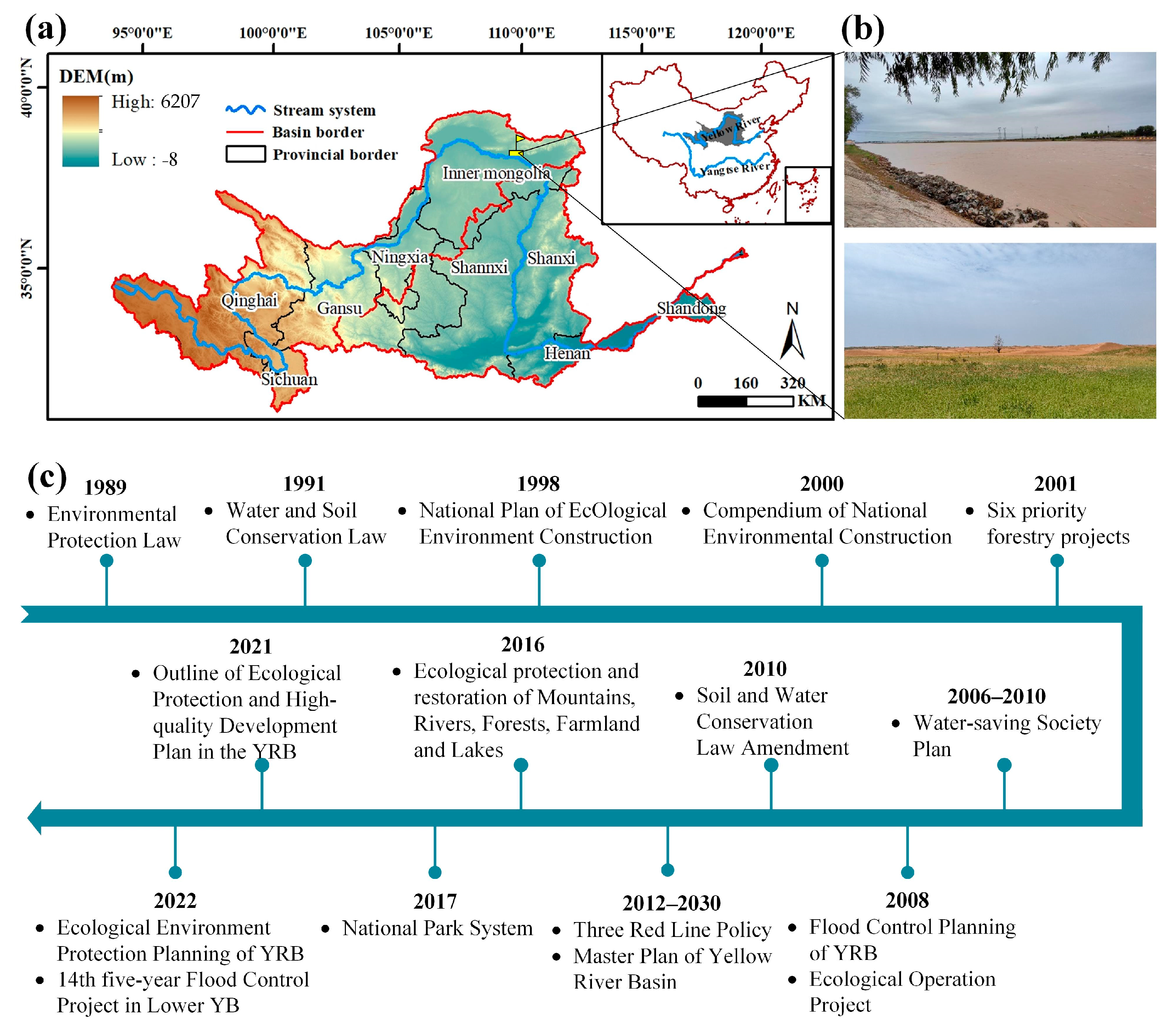
2.1. Study Area

The Yellow River Basin is located in northern China (95°53′~119°15′E, 32°10′~41°50′N) and covers a total area of 795,000 km² (Figure 1a). It is the second-largest basin and a critical ecosystem in China. The climate in the YRB transitions from arid and semi-arid in the northwest to semi-humid in the southeast. Precipitation is unevenly distributed, predominantly occurring between June and September, with average annual precipitation ranging from 140 mm to 1200 mm. The average annual evaporation is 1100 mm. The upstream region serves as the primary water-producing area, supplying freshwater resources for the agricultural and industrial needs of the YRB. The midstream and upstream regions include the Loess Plateau, one of the most serious soil erosion areas in the world [39]. The soil in this area is loose and the slopes are steep. Sparse vegetation and frequent rainstorms in summer lead to serious wind–sand erosion, soil erosion in the basin, and high sediment concentration in the river (Figure 1b). In addition, the YRB is located in arid and semi-arid areas with severe water shortages. In recent years, the overdevelopment of agriculture has led to a further increase in irrigation water, over-exploitation of groundwater, and a decrease in soil organic matter, which have brought tremendous pressure on the sustainable development of the regional ecological environment [40].

2.2. Dataset and Preprocessing

We collected multi-source remote sensing data, soil data, meteorological station data, and future meteorological model data. The detailed categories, years, and sources of the datasets are listed in

Table 1. Multi-source dataset information and their sources used in this study.

Data	Data Type	Data Product	Year	Resolution	Sources
MODIS	LULC	MCD12Q1	2010, 2020	500 m	https://ladsweb.modaps.eosdis.nasa.gov/ (accessed on 5 January 2024)
	NDVI	MOD13A3	2020	1000 m
	ET/PET	MOD16A2	2010–2020	500 m
Meteorological station	PRE	China Surface Meteorological Observation Dataset (Monthly)	2010–2020	Spatially interpolated to 1000 m	https://data.cma.cn/ (accessed on 5 January 2024)
	TEM
	WIN
SoilGrids	SOC	Soil Organic Carbon	—	250 m	https://soilgrids.org/ (accessed on 9 January 2024)
	Soil Texture	Clay content, Sand, Silt	—
SNPP	Night Light	NPP-VIIRS	2020	1000 m	https://www.resdc.cn/ (accessed on 12 January 2024)
SRTM	DEM	SRTM V4.1	—	90 m	https://www.gscloud.cn/ (accessed on 12 January 2024)
SEDAC	POP	Global 1-km Downscaled Population	2000–2100	1000 m	https://doi.org/10.7927/q7z9-9r69 (accessed on 18 January 2024)
CMIP6	Pre, Tem, Winds, GPP	CESM2	2001–2014, 2015–2100	1.25° × 0.94°	https://esgf-node.llnl.gov/search/cmip6/ (accessed on 18 January 2024)
		CNRM-CM6-1		1.41° × 1.41°
		CNRM-ESM2-1		1.41° × 1.41°
		TaiESM1		1.25° × 0.9°
		BCC-CSM2-MR		1.12° × 1.12°

.

2.2.1. Vegetation, Climate, and LULC Data

MCD12Q1, MOD13A3, and MOD16A2, from the Moderate Resolution Imaging Spectroradiometer (MODIS) of the National Aeronautics and Space Administration (NASA), are selected and applied for land use prediction and EV indicators calculation. LULC data (MCD12Q1) are simplified into eight categories, namely woodland, shrub, grassland, wetland, cropland, built-up, water, and others. The MOD13A3 dataset is a monthly Normalized Difference Vegetation Index (NDVI)/Enhanced Vegetation Index (EVI) product with a spatial resolution of 1000 m. Considering the sparse vegetation in the YRB, the overall vegetation coverage is low. NDVI is easily saturated in high coverage, but has obvious advantages in low coverage, which can better characterize the surface vegetation coverage information [41]. Thus, NDVI is selected to calculate the EV index in this study. The maximum value synthesis method and pixel dichotomy model are utilized to calculate the annual NDVI and vegetation coverage, respectively [42,43]. MOD16A2 is the Evapotranspiration (ET) product of MODIS, which is an accumulated 8-day composite data product with a spatial resolution of 500 m.

Meteorological data are obtained from the National Meteorological Data Center, including monthly average precipitation (PRE), temperature (TEM), and wind speed (WIN) data from each meteorological station in the YRB and surrounding areas. Anusplin interpolation software (V4.3) is employed to perform spatial interpolation on these meteorological station data, resulting in raster data with a spatial resolution of 1000 m.

Soil data are obtained from the Global Grid Soil Information System (SoilGrids), including soil organic carbon (SOC) and soil texture. Soil texture is divided into three categories: sand, silt, and clay. Soil conservation is calculated using the Revised Universal Soil Loss Equation (RUSLE) in this study [44].

Night light dataset is downloaded from the Resource and Environmental Science Data Platform (RESDP). This dataset is developed using the monthly products of the Suomi National Polar-orbiting Partnership Satellite VIIRS Sensor (NPP-VIIRS) with a spatial resolution of 1000 m. The denoising process of NPP-VIIRS data consists of two steps, and the specific steps are detailed in the Supplementary Materials. The first step is to remove background noise (abnormally low values). The second step is to correct for outliers (abnormally high values) that may be caused by short-lived light sources such as oil or gas fires [45,46,47].

Socioeconomic data, such as gross domestic product (GDP) and population density (spatial resolution of 1000 m), and ecological function protection area boundary data are downloaded from the RESDP. Current highway, railway, town point, and river datasets are acquired from the BIGEMAP map downloader. The digital elevation model (DEM) is obtained from the Shuttle Radar Topography Mission (SRTM). The DEM spatial resolution is 90 m and is used to extract the slope factor.

2.2.2. Projections Dataset

The combined scenario data of different Shared Socioeconomic Pathways (SSPs) and Representative Concentration Pathways (RCPs) of the latest Coupled Model Intercomparison Project Phase 6 (CMIP6) are applied in this study. This dataset emphasizes the driving effect of different socioeconomic development patterns on climate change [32,48]. We collected the simulation results dataset from the Earth System Models of five CMIP6 models (Table 1). These model data provide monthly precipitation, Gross Primary Productivity (GPP), air temperature, and wind speed, which are utilized for LULC prediction and vulnerability index calculation. Three scenarios—SSP1-2.6 (SSP1 and RCP2.6), SSP2-4.5 (SSP2 and RCP4.5) and SSP5-8.5 (SSP5 and RCP8.5)—are adopted in this study. Among these, historical data from 2001 to 2014 and simulation data from 2015 to 2019 are used to verify the CMIP6 model data. The scenario-predicted data for 2020–2070 are applied for future EV assessment. The average values of future climate change scenario precipitation data (2030–2070) are calculated at ten-year intervals (Figure S1). In addition, we adopt the multi-model average value of CMIP6 to overcome uncertainties between CMIP6 models [49,50].

Future population data are acquired from NASA’s Socioeconomic Data and Applications Center (SEDAC), which provides global gridded population data with a resolution of 1000 m. The dataset includes total population data for ten-year intervals in 2000 (base year) and 2010–2100 (forecast years), consistent with global population and urbanization predictions under different SSPs [51].

The multi-scenario monthly potential evapotranspiration (PET) dataset for China (2021–2100) is obtained from the Qinghai-Tibet Plateau Data Center. The spatial resolution of the data is 0.008° (about 1000 m), and the dataset is obtained using the Hargreaves PET calculation formula [52].

Considering the variances in the data sources and spatial accuracy of the datasets utilized in this study, the spatial resolution of datasets is resampled at 1000 m using the nearest neighbor resampling method [53,54]. This study applies the WGS 1984 coordinate system and UTM 43N projection to maintain the spatial consistency of all datasets.

2.3. Models and Processes

This study proposes an integrated EV assessment framework that combines Markov, PLUS, and E-S-A models (Figure 2). First, various future scenarios are designed by integrating the CMIP6 climate change scenario with LULC and ecological protection planning for the YRB, introducing the land use growth factor (i.e., scenario weight matrix) to optimize the Markov model. Second, the coupled Markov-PLUS models are utilized to distribute land use demand across various spatial distributions. Third, the E-S-A framework, along with an optimized index system, is employed to simulate and forecast EV under multiple future scenarios.

2.3.1. Multi-Scenarios in the Future

The implementation of ecological projects and policies, including the Grain-for-Green (GFG), the Natural Forest Protection (NFP), and the Three Norths Shelterbelt Project (TNSP), has significantly influenced the LULC structure in the YRB [35,55,56,57]. These initiatives have contributed to increased vegetation coverage and a reduction in soil erosion [58]. In the YRB, approximately 50% of the cropland consists of sloping land, with some slopes greater than 25° restored to forest and grassland under the GFG between 2000 and 2013 [59]. After the implementation of the GFG in Yanchuan County in the midstream of the YRB, above 46% of the cropland was converted to orchards and sparse forests. Nevertheless, the complex trade-off between the continued increase in forest and grassland and the dissipation of water resources remains challenging to effectively recognize and regulate.

Over the past 30 years, the urbanization rate of the Loess Plateau has risen by 30%, with Xi’an nearing an urbanization rate of 80%. Rapid urbanization and the encroachment on cropland have resulted in a decline in agricultural production potential. The Yellow River Basin Comprehensive Plan (2012–2030), the National Ecological Function Zoning (Revised Edition 2015) [60], the ecological red-line policy [61], and the Framework of the plan for ecological protection and high-quality development of the Yellow River Basin [62] pointed out that the YRB is facing issues of how to balance the relationship between urban development—cropland protection, ecological conservation—and water resources supply.

Due to changes in influencing factors, future land use simulations are fraught with uncertainty [63]. Scenario development provides a relatively realistic simulation of LUCC according to varying climatic conditions and socioeconomic factors, thereby offering guidance for land policy formulation [64,65]. This study synthesizes the land use management orientation of the relevant policy planning, and existing research [25,66,67], to construct a set of LULC development scenarios corresponding to the three combination scenarios of CMIP6, establishing growth factors for each scenario, namely Markov weight factors (

Table 2. The weight values (W_n) in different scenarios.

Scenarios	Weight Values (Wn)
Ecological conservation scenario (SSP1-2.6)	Diag (Woodland, Shrub, Grassland, Wetland, Cropland, Built-up, Water, Others) = (1.2, 1.1, 1.2, 1, 0.95, 0.85, 1, 1)
Historical trend scenario (SSP2-4.5)	―
Urban development scenario (SSP5-8.5)	Diag (Woodland, Shrub, Grassland, Wetland, Cropland, Built-up, Water, Others) = (0.9, 1, 0.9, 1, 1.1, 1.2, 1, 1)

). For example, 2 of the 1.2 in “Diag (Woodland, Shrub, Grassland, Wetland, Cropland, Built-up, Water, Others) = (1.2, 1.1, 1.2, 1, 0.95, 0.85, 1, 1)” represent a 20% increase in the change in woodland and grassland areas relative to historical trends (i.e., 2010–2020), while cropland and built-up areas are limited by policy and scenario settings, with reductions of 5% and 15%, respectively.

The ecological conservation management scenario (ECMS) corresponds to the SSP1-2.6 scenario. This scenario simulates the effectiveness of ecological land protection policies and measures, such as grazing bans and GFG initiatives, by moderately increasing forests and grasslands, mitigating cropland degradation, and limiting urban land expansion. For instance, GFG measures are implemented on cropland with slopes greater than 25°.

The historical trend scenario (HTS) corresponds to SSP2-4.5. This scenario employs the trend extrapolation method, positing that the current rate of LUCC will persist unchanged.

Urban development and construction scenario (UDCS) is designed to simulate the large-scale expansion of urban land and cropland, corresponding to the SSP5-8.5 scenario. This scenario simulates the urban expansion of population growth and cropland degradation by assuming an increase of 10% in the proportions of forest, grassland, and fallow land areas.

Furthermore, in the ECMS, nature reserves and ecological function reserves are designated as restricted areas for land expansion. In contrast, the UDCS operates without spatial limitations.

2.3.2. Spatiotemporal Modeling and Prediction of Land Use

(1)

Markov-PLUS-based land use modeling

The Markov chain is formed based on the Markov random process system. The primary method involves extracting the transition probability matrix (A_ij) of LULC over two periods to simulate LUCC. Markov chain exhibits high computational efficiency and robustness, and it has been widely utilized in various random process simulations and predictions [68,69].

$$A(t+1)=A(t)A_{ij}$$

(1)

where A(t + 1) and A(t) represent the state of LULC at times t + 1 and t, respectively, n is the total number of LULC types, and A_ij is the probability of the i-type transferring to the j-type.

Since A_ij is only related to the LULC type at time t and has no aftereffect, the probability matrix based on the initial LULC cannot predict LUCC under different development scenarios. Therefore, to simulate LULC under different scenarios, this study introduces the scenario weight matrix (W_n) based on the probability matrix of the initial LULC type.

$$A_{ij}^{\prime }=\left[\begin{array}{cccc}{A}_{11}& A_{12}& \cdots & A_{1n}\\ A_{21}& A_{22}& \cdots & A_{2n}\\ ⋮& ⋮& \ddots & ⋮\\ A_{n1}& A_{n2}& \cdots & A_{nn}\end{array}\right]\left[\begin{array}{llll}{w}_1& & & \\ & w_2& & \\ & & \ddots & \\ & & & w_n\end{array}\right]$$

(2)

$$A_{ij}^{″}=\left[\begin{array}{llll}{\displaystyle \raisebox{1ex}{$1$}\!\left/ \!\raisebox{-1ex}{${\displaystyle {\sum }_{k=1}^n{A}_{1k}^{\prime }}$}\right.}& & & \\ & {\displaystyle \raisebox{1ex}{$1$}\!\left/ \!\raisebox{-1ex}{${\displaystyle {\sum }_{k=1}^n{A}_{2k}^{\prime }}$}\right.}& & \\ & & \ddots & \\ & & & {\displaystyle \raisebox{1ex}{$1$}\!\left/ \!\raisebox{-1ex}{${\displaystyle {\sum }_{k=1}^n{A}_{nk}^{\prime }}$}\right.}\end{array}\right]\times A_{ij}^{\prime }$$

(3)

where $A_{ij}^{\prime }$ is the transfer matrix after the scenario weight W_n is applied and $A_{ij}^{″}$ is obtained after normalization. According to the specific W_n, multi-scenario LUCC is reflected. The improved Markov model is A(t + 1) = A(t)$A_{ij}^{″}$.

The Patch-generating Land Use Simulation model (PLUS) combines a rule-mining framework based on the Land Expansion Analysis Strategy (LEAS) with the Cellular Automata (CA) model using multi-type random seeds (CARSs) [66]. First, LEAS is utilized to extract the areas where LULC types have changed over two periods. Next, based on the random forest algorithm, LULC expansion is identified to determine the change law and development potential of different LULC types. The CARSs model simulates local LULC competition based on adaptive coefficients, neighborhood effect, and development probabilities, thereby dynamically generating patches. By coupling the PLUS model with a multi-objective optimization algorithm, the influence of various spatial factors is better combined with geographical units, resulting in higher simulation accuracy [70,71]. Furthermore, the PLUS model can simulate multi-type LUCC at the patch level, providing a more realistic landscape pattern. The modeling results more effectively support planning policies aimed at sustainable development [72].

In summary, the coupled Markov-PLUS model can accurately simulate the spatiotemporal changes in regional LULC under different policies or planning schemes by setting different scenarios. The coupled model requires a large amount of LULC data and driving factors as input, which may make the model construction and operation relatively complex. However, due to its strong universality and application value, the Markov-PLUS model has been widely used in the field of LUCC simulation and prediction [73,74,75], providing a theoretical reference for regional ecological environmental protection and effective resource utilization. Additionally, the model is not only applicable to high surface coverage areas such as urban agglomerations and small watersheds, but also to arid areas with low vegetation coverage.

(2)

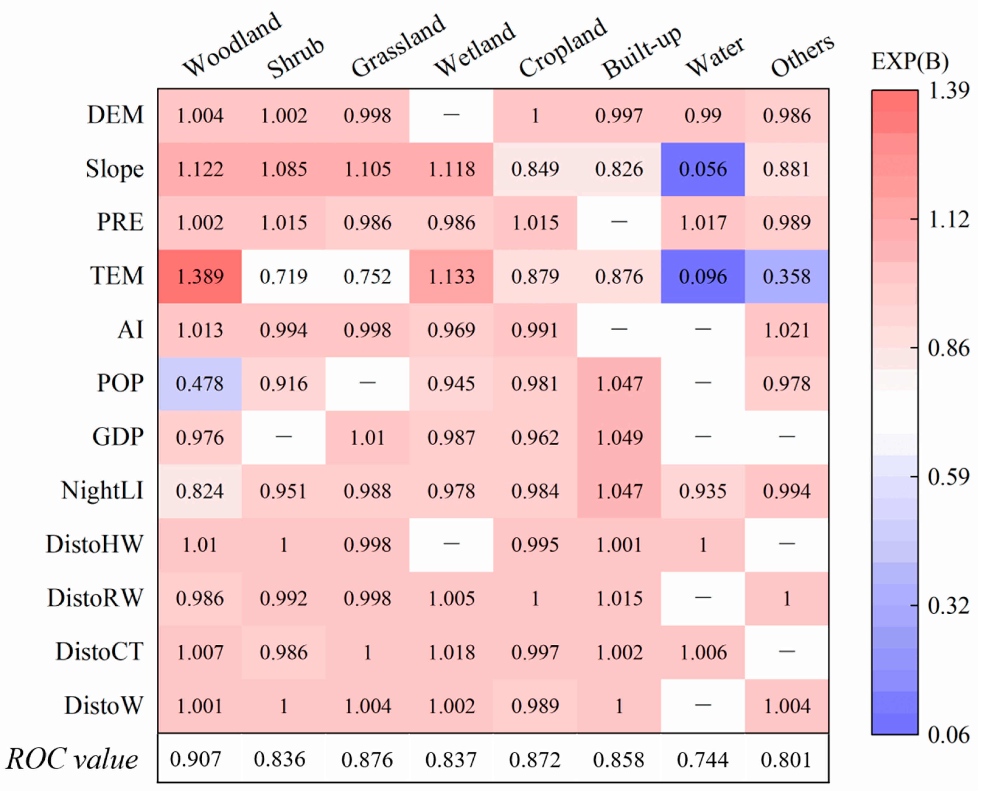
Selection of LUCC driving factors

The selection of driving factors for LUCC is a critical component of PLUS modeling. Population expansion, urbanization, excessive agricultural development, and ecological restoration policies substantially altered LUCC in the YRB. Drawing from previous studies [29,66,76], environmental factors such as slope, PRE, TEM, aridity index (AI), and socioeconomic factors like GDP, population density, and road networks are selected as driving factors for LUCC modeling in this study (Figure S2). Aridity index is the ratio of PER to PET (i.e., AI = PRE/PET), which is widely applied to assess drought conditions [77]. These twelve factors are input into the PLUS model as predictors to determine the suitability probability for each LULC type.

A logistic regression model is utilized to verify and identify potential driving factors of LULC [78]. Moreover, the receiver operating characteristic curve (ROC) method is utilized to test the goodness of fit for the logistic regression model. The area under the ROC curve represents the ROC value [79]. An ROC value closer to 1 indicates higher prediction accuracy. Generally, ROC > 0.7 indicates good interpretative accuracy.

2.3.3. Multi-Scenario Modeling and Assessment of Ecological Vulnerability

The exposure–sensitivity–adaptation (E-S-A) framework highlights the intrinsic causes of vulnerability and is widely used in ecological assessment [7,80,81]. This study primarily refers to the E-S-A evaluation index system, grading standards, and ESVI index calculation method constructed by Zhang et al. [15]. By further optimizing and improving specific indicators, this study evaluates future ecological vulnerability under different climate scenarios and ecological restoration policies (

Table 3. Evaluation index system of future ecological vulnerability in the YRB and their weight coefficients.

Overall Objective	First-Level Indicator (Weight)	Second-Level Indicator (Weight) (±)	Formula	Description
Ecological vulnerability	Exposure B1. (0.297)	Precipitation (0.524) (−)	$PR{I}_i={\displaystyle \frac{{\displaystyle {\sum }_{k=1}^{n}PR{E}_{ik}\times S_0}}{PR{E}_{i.\max }\times S_i}}$	X1. PREik is the annual PRE of the k-th pixel in the i-th grid; PREi.max is the maximum PRE in the i-th grid; S0 is the area of the pixel, which is 1 km2; Si is the area of the i-th grid.
		Terrain slope (0.197) (+)	$TS{I}_i={\displaystyle \frac{{\displaystyle {\sum }_{k=1}^{n}T{S}_{ik}\times S_0}}{90\cdot S_i}}\times \left({\sigma }_i/{\mu }_i\right)$	X2. TSik is the slope of the k-th pixel in the i-th grid; σi and μi are the slopes’ variance and mean values in the i-th grid, respectively.
		Population coefficient (0.279) (+)	$POP{C}_i=Po{p}_i\times {\displaystyle \frac{U_i}{S_i}}\times 100$	X3. Popi and Ui are the population density and built-up land area in the i-th grid, respectively.
	Sensitivity B2. (0.540)	Ecosystem elasticity (0.214) (−)	$EE{I}_i={\displaystyle \frac{{\displaystyle {\sum }_{p=1}^n{V}_{ip}\times S_{ip}}}{S_i}}$	X4. Vip and Sip are the elasticity coefficient and area of land use type p of the i-th grid.
		Ecosystem vitality (0.214) (−)	$EV{I}_i={\displaystyle \frac{{\displaystyle {\sum }_{k=1}^{n}GP{P}_{ik}\times S_0}}{GP{P}_{i.\max }\times S_i}}$	X5. GPPik is the GPP value of the k-th pixel in the i-th grid; GPPi.max is the largest GPP value in the i-th grid.
		Ecosystem services (0.286) (−) (+)	$A{c}_i=R_i\times K_i\times L{S}_i\times (1-C_i\times P_i)$	X6. Soil conservation (Ac): Ri and Ki are the rainfall erosivity and soil erodibility factors, respectively; LSi is the slope steepness and slope length factor; Ci and Pi are the vegetation coverage and governance measure factors, respectively.
			$E_i=Cw{e}_i\times {(8.2\times {10}^{-5})}^{C_i}$$Cw{e}_i={\displaystyle \frac{1}{100}}{\displaystyle {\sum }_{n=1}^{12}{w}_i^3\left(\frac{PE{T}_i-PR{E}_i}{PE{T}_i}\right)}$	X7. Wind–sand erosion (Ei). Cwei is the wind erosion and climate erosion factor; wi and PETi are the average wind speed and PET in the n-th month.
		Aridity stress (0.286) (+)	$VS{I}_i={\displaystyle \frac{{\displaystyle {\sum }_{k=1}^n\left(\frac{PR{E}_{ik}}{PE{T}_{ik}}\right)\times S_0}}{S_i}}$	X8. PREik and PETik are the annual PRE and PET of the k-th pixel in the i-th grid, respectively.
	Adaptability B3. (0.163)	Protected area coefficient (−)	$EP{I}_i={\displaystyle \frac{S_{i.EPI}}{S_i}}$	X9. Si.EPI is an ecological function protection zone area in the i-th grid.

).

Considering the availability of predicted data, such as future nighttime light data, NDVI and ET cannot be accurately simulated. In this study, average population density replaces the population aggregation coefficient in the human disturbance intensity index, and GPP is used to replace NDVI in the ecosystem vitality index. The essence of ecosystem vitality is the rate of ecosystem accumulation of dry matter, generally expressed by GPP or NPP. Therefore, it is reasonable to apply GPP to calculate ecosystem vitality. Ecological elasticity refers to the ability of an ecosystem to self-recover and adapt in the face of external disturbances [82]. Based on previous studies [15,82], the elasticity coefficient for various land use types in the YRB is determined by expert consultation as follows: Woodland and Shrub, 1; Grassland, 0.8; Wetland and water, 1; Cropland, 0.6; Built-up, 0.2; Others, 0.4. The YRB is highly sensitive to hydraulic and wind erosion [83]. Loose soil, sparse vegetation, and periodic heavy rainfall lead to severe soil erosion in the region. Moreover, there is a large amount of bare soil and sparse grassland in the northwest, and wind erosion is particularly serious in spring, autumn, and winter. Changes in LULC types and vegetation structure directly affect changes in ecosystem service functions in the basin. Therefore, this study chooses soil conservation and wind–sand erosion to characterize the changes in ecosystem service functions in the YRB under the combined effects of natural factors and human restoration measures. The detailed calculation process and related parameters for soil conservation can be found in the study by Zhang et al. [58]. The AI provides a measure of water availability for potential plant growth and offers an important baseline for measuring and predicting climate change and its impact on plant growth. Thus, AI is adopted to replace the vegetation water stress index. Moreover, the constructed future EV assessment indicator system integrates the ecological model with remote sensing data and future climate scenario data (precipitation, wind speed, and Gross Primary Production), developing and enriching the contents and methods for calculating exposure, sensitivity, and adaptability. This study assumes that the terrain slope and soil attribute in the YRB remain unchanged. In addition, the fuzzy analytic hierarchy process (FAHP) is utilized to calculate the weight of each indicator in Table 3. FAHP uses the fuzzy consistency matrix as the judgment matrix, which can better deal with the inaccuracy and ambiguity in indicator judgment. The specific weight calculation method and process are detailed by Zhang et al. and Xue et al. [15,81].

To depict the change characteristics of the comprehensive index of EV, this study adopts the relative change rate to capture the change in EVSI under future scenarios. Using the EVSI under the HTS as the baseline value, the relative change rates of the EVSI under the ECMS and UDCS are calculated and analyzed to reflect temporal changes in future EV under these two scenarios.

$$\alpha ={\displaystyle \raisebox{1ex}{$\left(EVS{I}_{k,j}-EVS{I}_{k,HTS}\right)$}\!\left/ \!\raisebox{-1ex}{$EVS{I}_{k,HTS}$}\right.}\times 100\%$$

(4)

where α represents the relative change rate of EVSI relative to the baseline scenario. EVSI_k,j represents the EVSI value of the ECMS and UDCS in different years, and EVSI_k,HTS represents the EVSI value under the HTS in the corresponding year.

Population is an important influencing factor in LULC analysis and EV assessment. If the regional ecological environment remains fragile for a prolonged period, it will inevitably have a negative impact on sustainable human development and economic growth. This study adopts the CMIP6 dataset to estimate the population affected by the expansion of EV by overlaying future population data onto different levels of ecologically vulnerable areas. To explore the potential influence of climate change on the population in vulnerable areas, this study analyzes the population changes within these areas over time under the three future scenarios (ECMS, HTS, UDCS).

3. Results

3.1. Parameter Selection and Accuracy Verification

Before simulating LULC in future scenarios, we verify the selected 14 driving factors and the PLUS model. Logistic regression analysis is performed for each land type in relation to selected driving factors to test their influence on LULC (Figure 3). EXP(B), the occurrence ratio, is a key index for measuring the influence of explanatory variables on dependent variables. The EXP(B) of driving factors for woodland is TEM (1.389) > Slope (1.122) > AI (1.013) > DistoHW (1.007), indicating that the influence of temperature, slope, and drought degree is significant. Similarly, slope has the most significant effect on shrubs and grasslands. The driving factors that have an obvious impact on built-up land are POP, GDP, and nighttime light index. Furthermore, Figure 3 shows that the ROC value of woodland is the highest (ROC_woodland = 0.907), followed by grassland (ROC_grassland = 0.876). Although more than half of the driving factors have little effect on water (EXP(B) is less than 0.1 or eliminated), the ROC_water value reaches 0.744. In general, the ROC values for each LULC type are greater than 0.7, indicating that the regression model is appropriate and the 14 driving factors have good explanatory power for LULC modeling in the YRB.

Based on the above driving factors, the LULC data from 2010 is utilized to simulate the LULC for 2020, thereby verifying the applicability of the PLUS model in the YRB (Figure 4a,b). The model accuracy demonstrates that the PLUS model effectively simulates dynamic LUCC in the YRB. Specifically, the Kappa coefficient of PLUS is 0.85, and the overall accuracy is 92.42%. Further analysis of the producer accuracy (PA) of different LULC types shows that the PAs of cropland (98.20%), others (96.35%), woodland (96.20%), and grassland (90.62%) are above 90%. Due to the area of shrub and wetland accounting for less than 0.3%, the PAs of the two are low, at 69.87% and 72.41%, respectively.

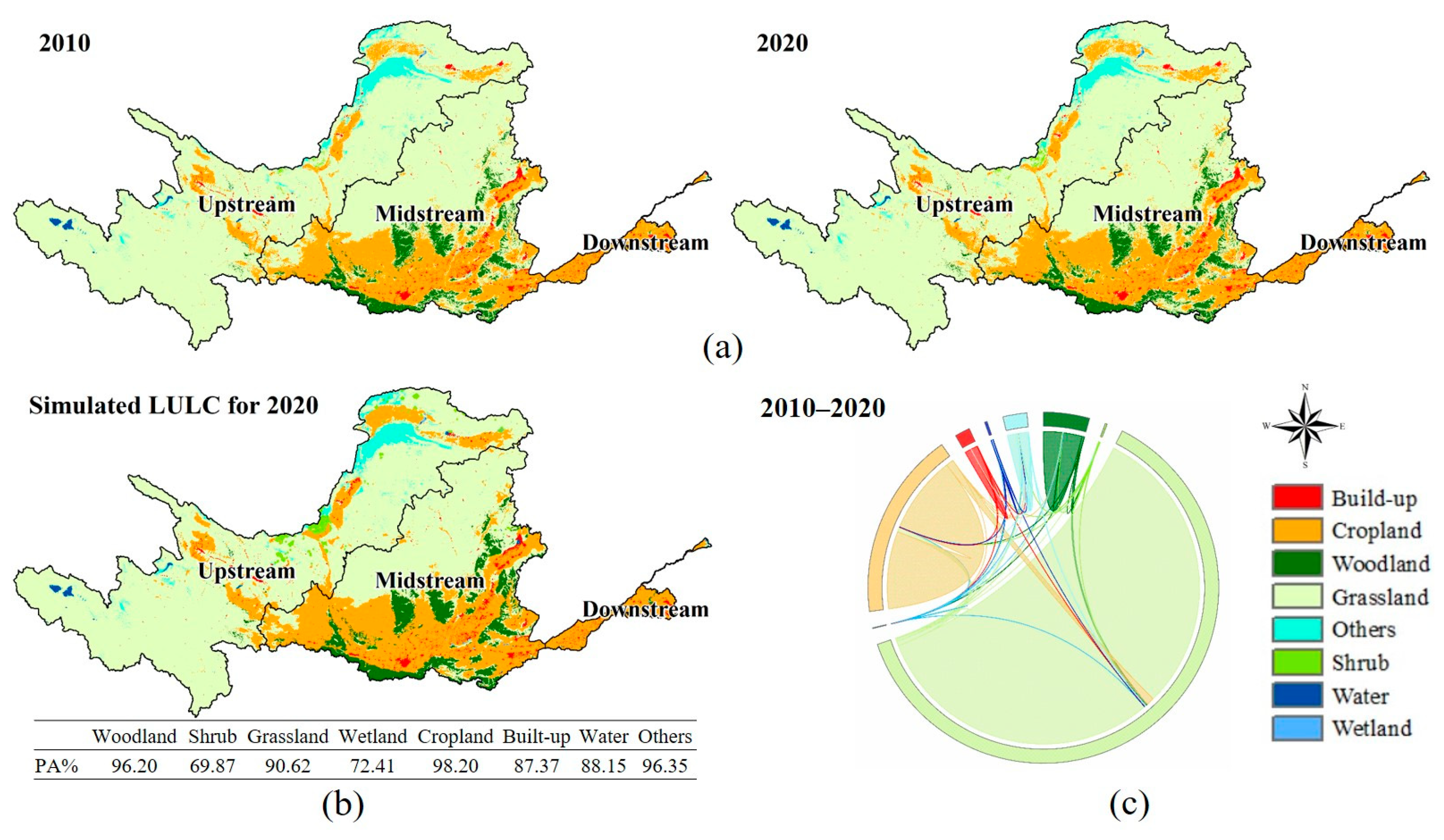
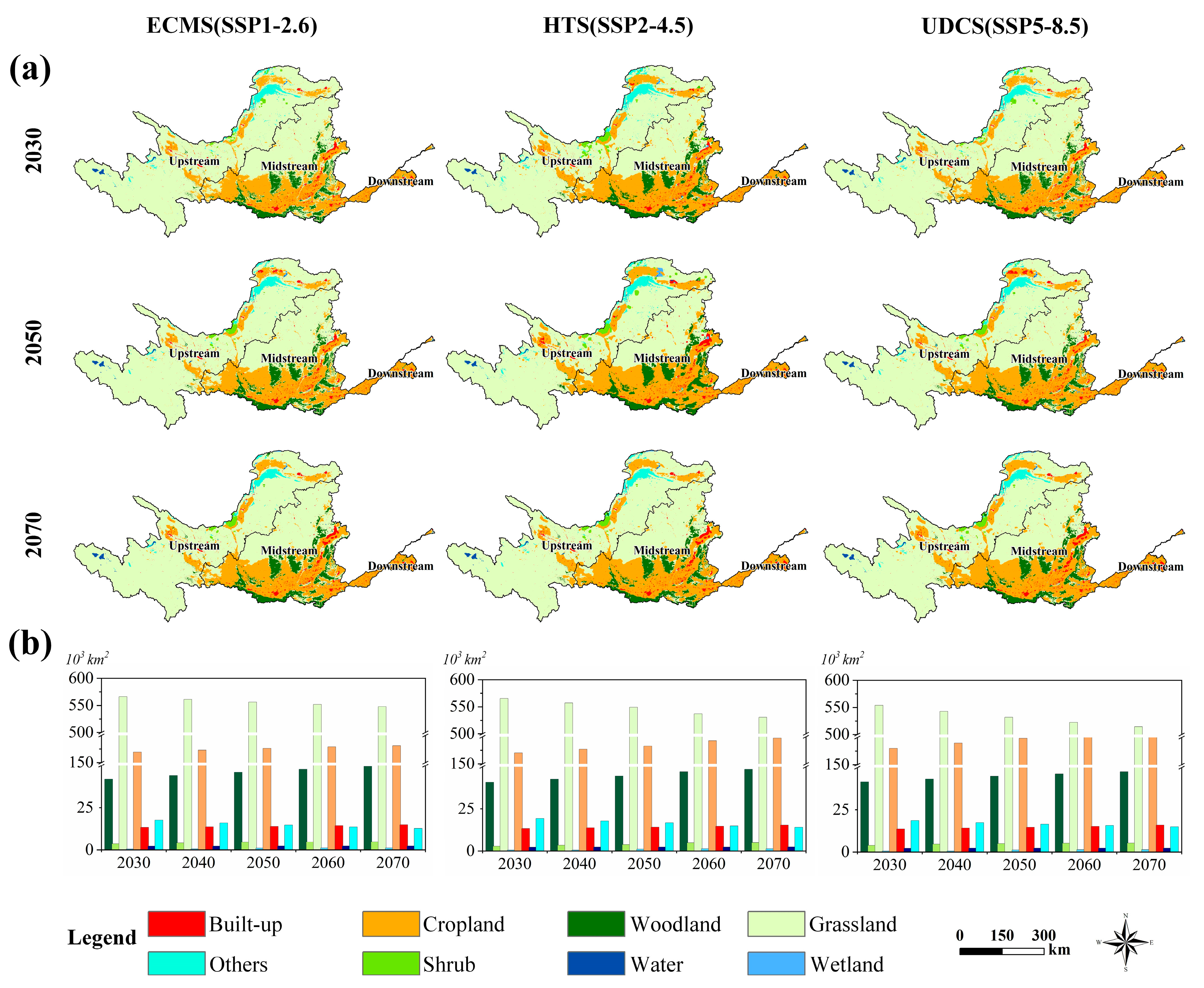
3.2. LUCC during 2010–2020 and under Three Development Scenarios

The LULC types in the YRB are primarily grassland, cropland, and woodland, accounting for 70.4%, 20.0%, and 5.1%, respectively, in 2020 (Figure 4). Grassland is widely distributed, concentrated in the high mountainous areas upstream and the desert areas midstream and upstream. The woodland in the midstream is densely distributed and extends to the north of the midstream. Cropland is mainly distributed in the valley plain in the south of the midstream and downstream region. These areas are flat and have favorable climatic conditions. From 2010 to 2020, 4.78% of the area’s LULC types have changed in the YRB. Figure 4a,c indicate that the most significant LUCC is the mutual conversion between grassland, woodland, cropland, and built-up land. In the increment of woodland, grassland accounts for the largest proportion, at 0.52%. With the implementation of the GFG project, cropland is mainly transferred to grassland and woodland (1.10% and 0.04%, respectively). However, the expansion of cropland and the acceleration of urbanization have caused a large area of grasslands to be occupied, resulting in a negative growth in grasslands (−0.85%). The main manifestations of land use changes from 2010 to 2020 in YRB are forest restoration, cropland expansion, and urbanization.

The LULC simulation results from 2030–2070 indicate substantial differences in local areas of the YRB under three future scenarios, particularly at the intersection of woodland, grassland, built-up land, and cropland (Figure 5a). Under the HTS, cropland expanded into grassland, while shrub and wetland areas remained relatively intact. The woodland in the eastern part of the midstream presented a certain degree of expansion, and built-up land showed a trend of expanding into cropland in the southern region. Under the ECMS, woodland and shrubs increased significantly. Moreover, the trend of grassland degradation slowed, indicating that the effect of ecological engineering is substantial. Compared with the HTS, the expansion of cropland is significantly reduced, particularly in the gully region of the Loess Plateau in the midstream. Under the UDCS, cropland in the southern part of the midstream is largely occupied, and there is spatial overlap with the increase in ecological land. In general, there is a notable relationship between rapid urbanization, ecological protection, and economic development.

There are significant variances in areas with different LULC from 2030 to 2070. The woodland and shrub areas increased under the three scenarios, with the trend of increasing woodland being ECMS (7465.5 km²) > HTS (6845.25 km²) > UDCS (6646.5 km²) (Figure 5b). Cropland and built-up land increased under all three scenarios, with the largest areas under UDCS (32,902.75 km² and 2174.25 km², respectively). Grassland showed varying degrees of decline under the three scenarios. Conversely, the extent of water and wetland areas showed varying degrees of increase.

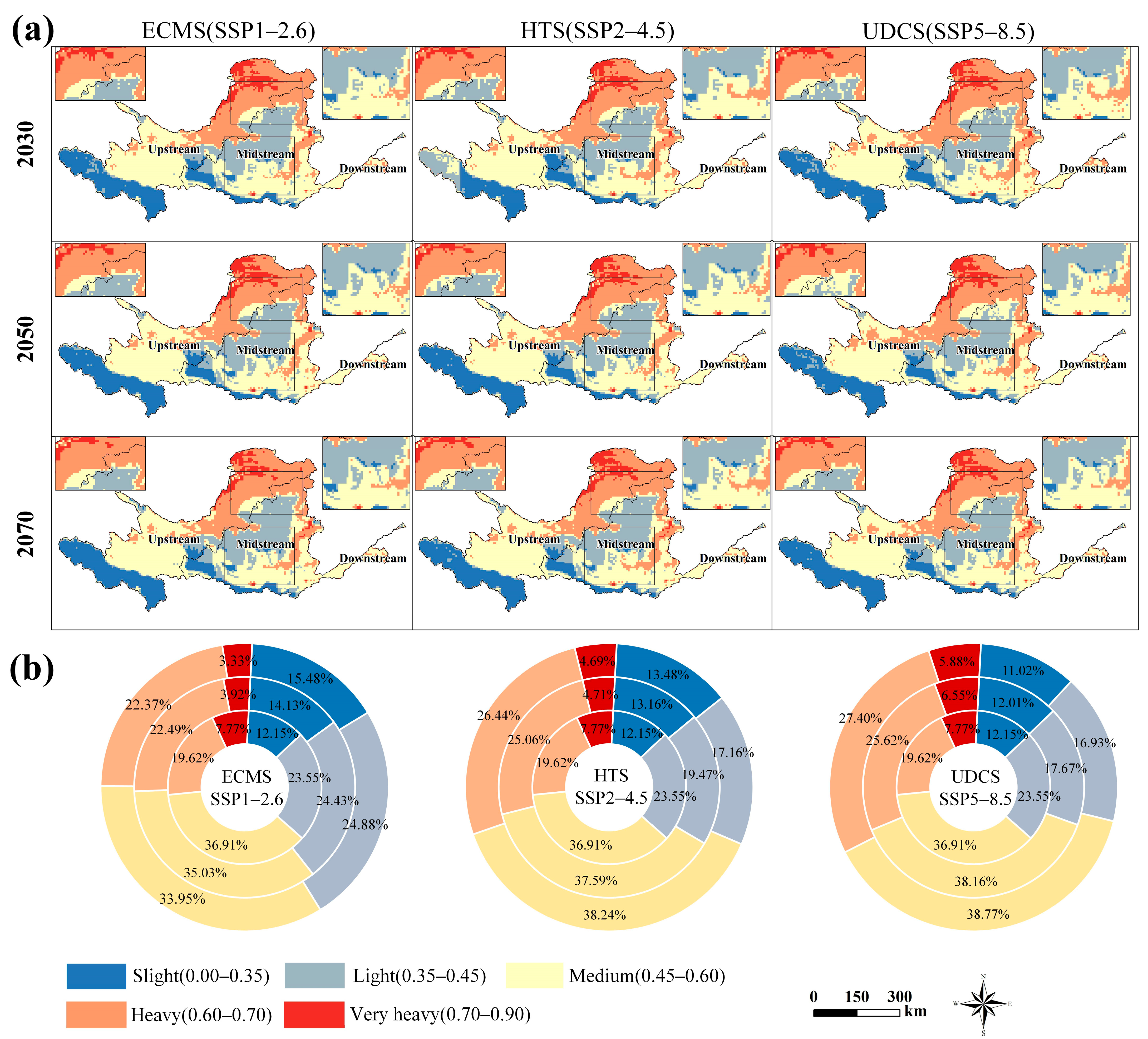
3.3. Multi-Scenario Assessment and Changes in Future EV

By integrating the Markov-PLUS and E-S-A model framework, we forecast the future (2030–2070) EV spatial patterns and changes in the YRB under the ECMS, HTS, and UDCS scenarios at a 10 km × 10 km grid scale (Figure 6). The spatial pattern of future EV in the three scenarios is consistent, while there are obvious geographical spatial differences in the vulnerability levels (Figure 6a). Consistent with the spatial distribution pattern of EV in 2020 (Figure S3), the northern part of the upstream YRB remains the region with a very heavy EV level over the next fifty years. Areas with heavy EV levels are mainly located in the middle of the upstream and east of the midstream. These vulnerability regions are consistent with those published by the Ministry of Ecology and Environment [84,85]. Affected by the monsoon climate, the community structure in the central and northern parts of the YRB is complex, with less precipitation and severe sand and soil erosion [86,87]. These conditions have led to the sensitivity of the regional ecosystem and poor resilience.

Under the ECMS, areas with reduced vulnerability are mainly distributed in the water conservation areas in the west of the upstream and the key areas of the GFG and NFP in the midstream. Under the HTS, the regions with decreased EV are similar to those under the ECMS, while the contribution of the ecological land expansion area is significantly lower. Under the UDCS, areas with increased vulnerability outnumber those with decreased vulnerability. These regions are mainly distributed in areas where cropland expands into grassland in the north and southeast of the YRB, and in areas where urban land expands into cropland or unused land.

To highlight the changes in EV, we compare the different levels of EV in 2040 and 2060 with those in 2020. Figure 6b shows that a large proportion of areas (above 33%) have a medium EV level in the YRB. Next are the areas with heavy and light EV levels, the trends of area proportions are opposite and vary significantly among the three future scenarios.

Under the HTS, the percentage of areas with slight EV levels will continue to increase in 2020–2040 and 2040–2060, with increases of 1.01% and 0.32%, respectively. The percentage of areas with medium and heavy EV levels will also increase. However, the proportion of areas with very heavy EV levels will be reduced by 3.06% and 0.02%, respectively. All of these indicate that the ecological environment under the HTS is gradually recovering, albeit at a very slow pace.

Under the ECMS, the percentage of areas with slight and light EV levels increases in 2020–2040 and 2040–2060 (1.98% and 1.35%, respectively). Moreover, the proportion of areas with medium and very heavy EV levels will decrease. This is due to enhanced precipitation in the midstream and downstream, as well as increased woodland and shrubs in the northern upstream region. Under the UDCS, the percentage of areas with slight and light EV levels decreases. Compared with the other two scenarios, the proportion of areas with light EV levels will decrease significantly from 2020 to 2040 and from 2040 to 2060 (5.88% and 0.74%, respectively). On the contrary, the percentage of areas with medium and heavy EV levels will increase rapidly by 1.25% and 0.61% from 2020 to 2040, and by 6.00% and 1.79% from 2040 to 2060, respectively.

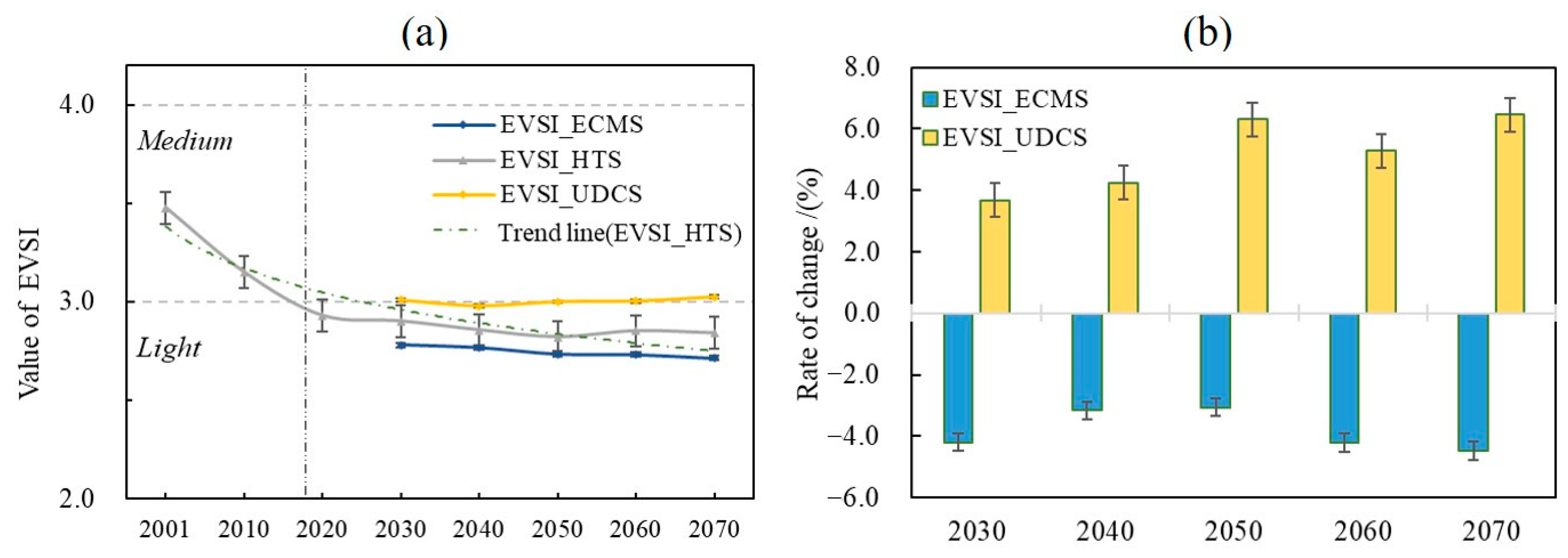
3.4. Analysis of Changes in and Influence of Future EV

To illustrate the impact of future climate change and LULC development on ecological vulnerability, this study used the historical trend scenario EVSI as a baseline to analyze EVSI changes in the YRB under the ECMS and UDCS scenarios from 2030 to 2070 (Figure 7a,b).

The vulnerability of the basin continues to decline slowly from 2030 to 2070 under the ECMS and HTS. By 2070, the EVSI under the ECMS is 2.72, showing a change rate of −4.48% compared to the EVSI under the HTS in the same year. In the HTS, the EVSI measures 2.84 in 2070, which is 0.06 lower than that in 2030 and 0.08 lower than under ECMS. This is due to significant woodland expansion expected under the ECMS over the next 50 years, while built-up land increases at a slower rate compared to the other scenarios (Figure 5b). This is consistent with the fact that the stability of forests and farmland is greater than that of built-up land. Similar patterns have been observed in previous studies [88,89].

The EVSI exhibits an overall upward trend under the UDCS in the YRB, which is detrimental to the restoration of the ecological environment. From 2030 to 2040, the EVSI decreases slightly, followed by a continued increase thereafter. By 2070, the overall EVSI increases by 0.02 compared to 2030, with a change rate of 6.47%, indicating gradual ecological deterioration under this scenario in the YRB.

Comparing the future population across different EV levels under the three scenarios reveals that the medium and heavily vulnerable areas contain a substantial proportion of the affected population, with the UDCS showing the highest impact (Figure 8). This trend correlates with the significant presence of areas with slight and light ecological vulnerabilities, coupled with the concentration of populations in the middle and lower reaches of the study area (Figure 6 and Figure S2). By 2040, the total affected population in medium and heavily vulnerable regions reaches 65.0 million, 66.47 million, and 67.02 million under ECMS, HTS, and UDCS, respectively. In 2060, a slight decline is observed, with affected populations of 55.7 million, 57.9 million, and 60.3 million under ECMS, HTS, and UDCS, respectively. From 2020 to 2060, despite a decline in population within the very heavily vulnerable areas across all three scenarios, the affected population is projected to remain above 5.1 million by 2060. In this sense, ecosystem degradation and population expansion in ecologically vulnerable areas are expected to be primary challenges for the high-quality development of the region in the future.

Populations in the slightly and lightly vulnerable areas (4.8 million and 9.0 million) are higher under the UDCS compared to the other scenarios from 2040 to 2060. Conversely, the population in the very heavily vulnerable areas (5.1 million) is lower than in the HTS (5.5 million) and ECMS (5.3 million). Hence, restoring ecological vulnerability and fostering sustainable socioeconomic development remain long-term challenges in the YRB.

4. Discussion

4.1. Ecological Vulnerability Assessment Rationality and Reliability

Using multi-source remote sensing, LULC, and CMIP6 multi-mode scenario data, this study analyzes the spatiotemporal evolution of LULC and EV in the YRB under three future scenarios. Based on CMIP6 multi-model average data for PRE, WIN, GPP (historical data: years 2001 and 2010; forecast data: 2020 for SSP2-4.5) and population data (historical data: year 2000; forecast data: 2010 and 2020 for SSP2-4.5), we calculate the EV for 2001, 2010, and 2020, and unify the results as the simulation results in HTS (Figure 7a). Findings reveal a consistent downward trend in EV from 2001 to 2020, reaching medium levels by 2020. These findings, alongside the EV spatial patterns depicted in Figure S3, align closely with those reported by previous research [15]. Therefore, the optimized E-S-A evaluation framework and CMIP6 model-simulated meteorological and population data perform well in simulating the EV.

The influence of climate change and human policies on EV under different future scenarios is complex and far-reaching. ECMS and UDCS represent contrasting scenarios: one emphasizing ecological protection (ECMS) and the other focusing on economic development (UDCS). Under the ECMS, climate change exhibits mild effects, and ecological lands such as woodland, shrubland, and grassland are protected, thereby contributing to reduced EV. Conversely, under the UDCS, intensified human activities, including urban and cropland expansion, alongside shifts in vegetation patterns and surface water resources due to climate warming, lead to ecological degradation and exacerbated EV. This issue is particularly acute in urban centers, suburbs, and their surrounding areas. Our findings corroborate those of Deng et al. [25], indicating that urbanization expansion results in substantial growth of artificial surfaces, thereby exacerbating regional ecological risks.

In the HTS, despite ongoing extensive ecological protection and restoration efforts, there has been a noticeable increase in built-up land and cropland, leading to limited improvement in EV. Recent research has highlighted that farmland reclamation significantly diminishes the effectiveness of ecological restoration [90]. Furthermore, rapid urbanization is related to current social and economic development trends, and the expansion of cropland correlates closely with population growth and food production. As human activities and climate change become more frequent in the future, EV intensity could potentially increase. Therefore, this study provides valuable insights into identifying potential vulnerability areas under various climate change and land development policy scenarios, facilitating the development of sustainable ecosystem management strategies for the YRB.

4.2. Insights for Future Development and Management of the YRB

This study attempts to explore LUCC and future EV evolution from the perspective of climate change, land management, and ecological protection policies. Scenario analysis reveals that human-related pressures significantly impact EV. In the UCDS, rapid urban and economic development will continuously increase EV and gradually deteriorate the ecological environment. Rapid climate change negatively impacts vegetation growth [66,91], altering the hydrological cycle and surface runoff patterns, and further aggravating rainfall-induced soil erosion. Additionally, the expansion of built-up land and cropland is driven by economic development and population growth, respectively [92]. Therefore, timely adjustment of socioeconomic development policies, slowing the pace of economic growth and climate change, and promoting the transformation of economic development from “high speed” to “high quality” may improve the fragile ecological environment of the YRB. Emphasizing the rationalization of landscape patterns, adopting a low-carbon new urbanization model, and optimizing LULC structure are effective strategies for the basin to cope with future climate change.

Under the HTS and ECMS, the EVSI will not increase in the YRB, but its degree of weakening is very limited (Figure 7a). Moreover, the population in high and very high vulnerability areas is projected to constitute 32.75–33.68% and 34.59–39.21% of the YRB’s total population in 2040 and 2060, respectively (Figure 8), and this proportion may continue to grow. Therefore, future ecosystem management of the YRB should balance economic and ecological considerations. Building on previous research results [15,89], the continued and increased implementation of GFG, NFP, and other projects is crucial for future ecosystem restoration in the YRB. Enhancing the connectivity of forests, grasslands, and wetlands can improve ecosystem services, resistance, and resilience [93]. Additionally, given future climate change and factors such as loose soil and serious soil erosion in arid and semi-arid areas, tree species and plants with developed root systems, drought resistance, and poor soil resistance should be prioritized. It is crucial to coordinate vegetation restoration with water resource management [18].

In view of the different vulnerability manifestations in the upper, middle, and lower reaches of the YRB, differentiated zoning protection and governance measures should be scientifically formulated according to local conditions. For instance, efforts should focus on upstream water conservation, midstream soil and water conservation, pollution control, and downstream wetland protection and restoration. It is important to note that the northern part of the upstream region serves as a barrier to wind–sand erosion in China, and its ecosystem is relatively uniform but highly vulnerable. Therefore, attention should be given to the spatial layout of vegetation structure and the construction of sand-fixing forest belts to enhance the quality of forests and grasslands and their ecosystem regulation functions.

4.3. Strengths and Limitations

Based on the climate change scenario of CMIP6 and LULC policy planning, this study designed future development scenarios, optimized the Markov-PLUS model with the aid of scenario weight matrix, and dynamically simulated the spatial distribution pattern and change characteristics in LULC in the YRB from 2030 to 2070. On this basis, the Markov-PLUS–ESA model framework is further proposed for modeling the EV under different future scenarios from the perspective of climate change, land management, and ecological protection policies. The inherent complexity, dynamics, and uncertainty of the future ecosystem in YRB highlight the necessity of further enhancing theoretical and practical research.

However, we acknowledge that this study has some limitations that can be addressed by future research. First, the YRB spans three climatic zones, resulting in complex and diverse ecosystem types. Different ecosystem types exhibit unique characteristics and varying responses to topography and precipitation. Moreover, these ecosystems play distinct and irreplaceable roles in ecological protection and restoration. Future research should further subdivide ecosystem types and assess and optimize within these subdivisions, such as farmland, grassland, and woodland vulnerabilities. Moreover, the setting and calculation of the elasticity coefficients are limited by the LULC type in this study. In the future, the elasticity differences between different types of forests, grasslands, and farmland should be fully considered to improve the accuracy of assessment results. The calculation of wind–sand erosion does not account for the soil and terrain factors, and the calculation of soil conservation and the LS factor is limited by the spatial resolution of the data, which affect the accuracy of the research results to a certain extent. Second, this study unifies the data resolution to 1000 m by resampling or downscaling techniques, which inevitably introduces uncertainty. Especially for the future climate model data with coarse resolution, it may not be able to fully simulate the small-scale physical processes due to the inherent defects of the original data model. Future research should further explore more advanced downscaling and upscaling methods and integrate multi-source high-resolution data to ensure the accuracy and reliability of climate prediction and EV evaluation while improving computational efficiency. Third, 0 and 1 only represent the relative lowest and highest EV levels in the YRB in this study. Therefore, the EV index and ranking obtained in this study only have direct comparative significance within the basin and may not be directly compared with other basins or wider geographical areas. Additionally, this study combines only three widely used and representative economic development and climate change scenarios [94,95], which may not fully reflect all possible future development directions. In future work, more SSP-RCP scenarios and policy demands should be considered to design more comprehensive scenarios and gain a deeper understanding of the future evolution of LULC and EV.

5. Conclusions

By designing future development scenarios, optimizing the Markov-PLUS model, and integrating the E-S-A framework, this study systematically predicted the spatiotemporal variation in LULC and EV in the YRB under different scenarios from 2020 to 2070 and their potential impact on future populations. Our research indicates that the overall spatial distribution pattern of LULC over the next 50 years remains relatively consistent across the three scenarios, with significant variations in specific local areas, particularly at the intersections of woodland and grassland, built-up land, and cropland. The northern part of the upstream watershed continues to exhibit very high vulnerability. Under ECMS, land protection measures and ecological policies significantly improve EV, reducing vulnerability by 0.22 between 2020 and 2070. In HTS, vulnerability shows a slight decrease (0.09), though the reduction is limited. Under UDCS, anthropogenic factors have a more pronounced impact, increasing the areas of medium and heavy vulnerability by 1.86% and 7.78%, respectively, posing a serious threat to ecosystem stability.

The affected population in medium and heavy vulnerability areas occupies a substantial proportion, especially under UDCS. Although the population in very high vulnerability areas shows a downward trend across all three scenarios from 2020 to 2060, the affected population will still exceed 5.1 million. Therefore, ecosystem degradation and population expansion in ecologically vulnerable areas are expected to be primary challenges for the region’s future high-quality development. Our research provides a valuable reference for future LULC planning, ecological restoration, and resource development in the YRB.

References

1. Feng, H.; Lei, X.; Yu, G.; Changchun, Z. Spatio-temporal evolution and trend prediction of urban ecosystem service value based on CLUE-S and GM (1,1) compound model. Environ. Monit. Assess. 2023, 195, 1282. [Google Scholar] [CrossRef] [PubMed]
2. IPCC. Climate Change 2022—Impacts, Adaptation and Vulnerability: Working Group II Contribution to the Sixth Assessment Report of the Intergovernmental Panel on Climate Change; Cambridge University Press: Cambridge, UK, 2023. [Google Scholar]
3. Nie, X.; Lu, B.; Chen, Z.; Yang, Y.; Chen, S.; Chen, Z.; Wang, H. Increase or decrease? Integrating the CLUMondo and InVEST models to assess the impact of the implementation of the Major Function Oriented Zone planning on carbon storage. Ecol. Indic. 2020, 118, 106708. [Google Scholar] [CrossRef]
4. Shirmohammadi, B.; Malekian, A.; Salajegheh, A.; Taheri, B.; Azarnivand, H.; Malek, Z.; Verburg, P.H. Impacts of future climate and land use change on water yield in a semiarid basin in Iran. Land Degrad. Dev. 2020, 31, 1252–1264. [Google Scholar] [CrossRef]
5. Graves, R.A.; Pearson, S.M.; Turner, M.G. Species richness alone does not predict cultural ecosystem service value. Proc. Natl. Acad. Sci. USA 2017, 114, 3774–3779. [Google Scholar] [CrossRef] [PubMed]
6. Dong, N.; You, L.; Cai, W.J.; Li, G.; Lin, H. Land use projections in China under global socioeconomic and emission scenarios: Utilizing a scenario-based land-use change assessment framework. Glob. Environ. Chang. 2018, 50, 164–177. [Google Scholar] [CrossRef]
7. Jiang, L.; Huang, X.X.; Wang, F.T.; Liu, Y.C.; An, P.L. Method for evaluating ecological vulnerability under climate change based on remote sensing: A case study. Ecol. Indic. 2018, 85, 479–486. [Google Scholar] [CrossRef]
8. Zhao, M.M.; He, Z.B.; Du, J.; Chen, L.F.; Lin, P.F.; Fang, S. Assessing the effects of ecological engineering on carbon storage by linking the CA-Markov and InVEST models. Ecol. Indic. 2019, 98, 29–38. [Google Scholar] [CrossRef]
9. He, L.; Shen, J.; Zhang, Y. Ecological vulnerability assessment for ecological conservation and environmental management. J. Environ. Manag. 2018, 206, 1115–1125. [Google Scholar] [CrossRef]
10. Chen, Y.; Xiong, K.N.; Ren, X.D.; Cheng, C. An overview of ecological vulnerability: A bibliometric analysis based on the Web of Science database. Environ. Sci. Pollut. Res. 2022, 29, 12984–12996. [Google Scholar] [CrossRef]
11. Ager, A.A.; Day, M.A.; Vogler, K. Production possibility frontiers and socioecological tradeoffs for restoration of fire adapted forests. J. Environ. Manag. 2016, 176, 157–168. [Google Scholar] [CrossRef]
12. Caballero, C.B.; Biggs, T.W.; Vergopolan, N.; West, T.A.P.; Ruhoff, A. Transformation of Brazil’s biomes: The dynamics and fate of agriculture and pasture expansion into native vegetation. Sci. Total Environ. 2023, 896, 166323. [Google Scholar] [CrossRef] [PubMed]
13. Liu, L.J.; Liang, Y.J.; Hashimoto, S. Integrated assessment of land-use/coverage changes and their impacts on ecosystem services in Gansu Province, northwest China: Implications for sustainable development goals. Sustain. Sci. 2020, 15, 297–314. [Google Scholar] [CrossRef]
14. Folke, C. Resilience: The emergence of a perspective for social–ecological systems analyses. Glob. Environ. Chang. 2006, 16, 253–267. [Google Scholar] [CrossRef]
15. Zhang, X.; Liu, K.; Wang, S.; Wu, T.; Li, X.; Wang, J.; Wang, D.; Zhu, H.; Tan, C.; Ji, Y. Spatiotemporal evolution of ecological vulnerability in the Yellow River Basin under ecological restoration initiatives. Ecol. Indic. 2022, 135, 108586. [Google Scholar] [CrossRef]
16. Li, Q.; Shi, X.; Wu, Q. Effects of protection and restoration on reducing ecological vulnerability. Sci. Total Environ. 2021, 761, 143180. [Google Scholar] [CrossRef]
17. Peng, B.; Huang, Q.; Elahi, E.; Wei, G. Ecological Environment Vulnerability and Driving Force of Yangtze River Urban Agglomeration. Sustainability 2019, 11, 6623. [Google Scholar] [CrossRef]
18. Liu, X.; Li, H.; Wang, S.; Liu, K.; Li, L.; Li, D.; Jia, A. Ecological Security Assessment of “Grain-for-Green” Program Typical Areas in Northern China Based on Multi-Source Remote Sensing Data. Remote Sens. 2023, 15, 5732. [Google Scholar] [CrossRef]
19. Segnon, A.C.; Totin, E.; Zougmoré, R.B.; Lokossou, J.C.; Thompson-Hall, M.; Ofori, B.O.; Achigan-Dako, E.G.; Gordon, C. Differential household vulnerability to climatic and non-climatic stressors in semi-arid areas of Mali, West Africa. Clim. Dev. 2021, 13, 697–712. [Google Scholar] [CrossRef]
20. Shah, M.A.R.; Wang, X. Assessing social-ecological vulnerability and risk to coastal flooding: A case study for Prince Edward Island, Canada. Int. J. Disast. Risk Reduct. 2024, 106, 104450. [Google Scholar] [CrossRef]
21. Dai, X.; Feng, H.; Xiao, L.; Zhou, J.; Wang, Z.; Zhang, J.; Fu, T.; Shan, Y.; Yang, X.; Ye, Y.; et al. Ecological vulnerability assessment of a China’s representative mining city based on hyperspectral remote sensing. Ecol. Indic. 2022, 145, 109663. [Google Scholar] [CrossRef]
22. Gao, Q.; Guo, Y.; Xu, H.; Ganjurjav, H.; Li, Y.; Wan, Y.; Qin, X.; Ma, X.; Liu, S. Climate change and its impacts on vegetation distribution and net primary productivity of the alpine ecosystem in the Qinghai-Tibetan Plateau. Sci. Total Environ. 2016, 554–555, 34–41. [Google Scholar] [CrossRef] [PubMed]
23. Zheng, Y.; Wang, S.; Cao, Y.; Shi, J.; Qu, Y.; Li, L.; Zhao, T.; Niu, Z.; Yang, R.; Gong, P. Assessing the ecological vulnerability of protected areas by using Big Earth Data. Int. J. Digit. Earth 2021, 14, 1624–1637. [Google Scholar] [CrossRef]
24. Li, D.; Huan, C.Y.; Yang, J.; Gu, H.L. Temporal and Spatial Distribution Changes, Driving Force Analysis and Simulation Prediction of Ecological Vulnerability in Liaoning Province, China. Land 2022, 11, 1025. [Google Scholar] [CrossRef]
25. Deng, G.; Jiang, H.; Zhu, S.; Wen, Y.; He, C.; Wang, X.; Sheng, L.; Guo, Y.; Cao, Y. Projecting the response of ecological risk to land use/land cover change in ecologically fragile regions. Sci. Total Environ. 2024, 914, 169908. [Google Scholar] [CrossRef] [PubMed]
26. Ma, L.X.; Hou, K.; Tang, H.J.; Liu, J.W.; Wu, S.Q.; Li, X.X.; Sun, P.C. A new perspective on the whole process of ecological vulnerability analysis based on the EFP framework. J. Clean. Prod. 2023, 426, 139160. [Google Scholar] [CrossRef]
27. Xie, Z.L.; Li, X.Z.; Jiang, D.G.; Lin, S.W.; Yang, B.; Chen, S.L. Threshold of island anthropogenic disturbance based on ecological vulnerability Assessment-A case study of Zhujiajian Island. Ocean Coast. Manag. 2019, 167, 127–136. [Google Scholar] [CrossRef]
28. Kebede, A.S.; Nicholls, R.J.; Allan, A.; Arto, I.; Cazcarro, I.; Fernandes, J.A.; Hill, C.T.; Hutton, C.W.; Kay, S.; Lázár, A.N.; et al. Applying the global RCP–SSP–SPA scenario framework at sub-national scale: A multi-scale and participatory scenario approach. Sci. Total Environ. 2018, 635, 659–672. [Google Scholar] [CrossRef]
29. Zhang, K.L.; Fang, B.; Zhang, Z.C.; Liu, T.; Liu, K. Exploring future ecosystem service changes and key contributing factors from a “past-future-action” perspective: A case study of the Yellow River Basin. Sci. Total Environ. 2024, 926, 171630. [Google Scholar] [CrossRef]
30. Eyring, V.; Bony, S.; Meehl, G.A.; Senior, C.A.; Stevens, B.; Stouffer, R.J.; Taylor, K.E. Overview of the Coupled Model Intercomparison Project Phase 6 (CMIP6) experimental design and organization. Geosci. Model Dev. 2016, 9, 1937–1958. [Google Scholar] [CrossRef]
31. Coelho, S.; Rafael, S.; Fernandes, A.P.; Lopes, M.; Carvalho, D. How the new climate scenarios will affect air quality trends: An exploratory research. Urban Clim. 2023, 49, 101479. [Google Scholar] [CrossRef]
32. Li, S.Y.; Miao, L.J.; Jiang, Z.H.; Wang, G.J.; Gnyawali, K.R.; Zhang, J.; Zhang, H.; Fang, K.; He, Y.; Li, C. Projected drought conditions in Northwest China with CMIP6 models under combined SSPs and RCPs for 2015–2099. Adv. Clim. Chang. Res. 2020, 11, 210–217. [Google Scholar] [CrossRef]
33. Zhang, Q.; Zhang, Z.J.; Shi, P.J.; Singh, V.P.; Gu, X.H. Evaluation of ecological instream flow considering hydrological alterations in the Yellow River basin, China. Glob. Planet. Chang. 2018, 160, 61–74. [Google Scholar] [CrossRef]
34. Liu, Y.W.; Yuan, L. Study on the influencing factors and profitability of horizontal ecological compensation mechanism in Yellow River Basin of China. Environ. Sci. Pollut. Res. 2023, 30, 87353–87367. [Google Scholar] [CrossRef] [PubMed]
35. Omer, A.; Ma, Z.; Yuan, X.; Zheng, Z.; Saleem, F. A hydrological perspective on drought risk-assessment in the Yellow River Basin under future anthropogenic activities. J. Environ. Manag. 2021, 289, 112429. [Google Scholar] [CrossRef]
36. Yang, Y.; Li, H.; Qian, C. Analysis of the implementation effects of ecological restoration projects based on carbon storage and eco-environmental quality: A case study of the Yellow River Delta, China. J. Environ. Manag. 2023, 340, 117929. [Google Scholar] [CrossRef]
37. Liang, W.; Bai, D.; Jin, Z.; You, Y.C.; Li, J.X.; Yang, Y.T. A Study on the Streamflow Change and its Relationship with Climate Change and Ecological Restoration Measures in a Sediment Concentrated Region in the Loess Plateau, China. Water Resour. Manag. 2015, 29, 4045–4060. [Google Scholar] [CrossRef]
38. Zhu, M.; Zhang, X.; Elahi, E.; Fan, B.; Khalid, Z. Assessing ecological product values in the Yellow River Basin: Factors, trends, and strategies for sustainable development. Ecol. Indic. 2024, 160, 111708. [Google Scholar] [CrossRef]
39. Wu, Q.; Jiang, X.; Shi, X.; Zhang, Y.; Liu, Y.; Cai, W. Spatiotemporal evolution characteristics of soil erosion and its driving mechanisms—A case Study: Loess Plateau, China. Catena 2024, 242, 108075. [Google Scholar] [CrossRef]
40. Li, J. A simulation approach to optimizing the vegetation covers under the water constraint in the Yellow River Basin. For. Policy Econ. 2021, 123, 102377. [Google Scholar] [CrossRef]
41. Yang, J.; Guo, N. Ananlyses on MODIS-NDVI index saturation in Northwest China. Plateau Meteorol. 2008, 27, 896–903. [Google Scholar] [CrossRef]
42. Ge, J.; Meng, B.; Liang, T.; Feng, Q.; Gao, J.; Yang, S.; Huang, X.; Xie, H. Modeling alpine grassland cover based on MODIS data and support vector machine regression in the headwater region of the Huanghe River, China. Remote Sens. Environ. 2018, 218, 162–173. [Google Scholar] [CrossRef]
43. Zhou, Y.; Batelaan, O.; Guan, H.; Liu, T.; Duan, L.; Wang, Y.; Li, X. Assessing long-term trends in vegetation cover change in the Xilin River Basin: Potential for monitoring grassland degradation and restoration. J. Environ. Manag. 2024, 349, 119579. [Google Scholar] [CrossRef] [PubMed]
44. Thomas, J.; Joseph, S.; Thrivikramji, K.P. Assessment of soil erosion in a tropical mountain river basin of the southern Western Ghats, India using RUSLE and GIS. Geosci. Front. 2018, 9, 893–906. [Google Scholar] [CrossRef]
45. Zhao, M.; Zhou, Y.; Li, X.; Zhou, C.; Cheng, W.; Li, M.; Huang, K. Building a Series of Consistent Night-Time Light Data (1992–2018) in Southeast Asia by Integrating DMSP-OLS and NPP-VIIRS. IEEE Trans. Geosci. Remote Sens. 2020, 58, 1843–1856. [Google Scholar] [CrossRef]
46. Jing, X.; Shao, X.; Cao, C.; Fu, X.; Yan, L. Comparison between the Suomi-NPP Day-Night Band and DMSP-OLS for Correlating Socio-Economic Variables at the Provincial Level in China. Remote Sens. 2016, 8, 17. [Google Scholar] [CrossRef]
47. Sun, Y.; Zheng, S.; Wu, Y.; Schlink, U.; Singh, R.P. Spatiotemporal Variations of City-Level Carbon Emissions in China during 2000–2017 Using Nighttime Light Data. Remote Sens. 2020, 12, 2916. [Google Scholar] [CrossRef]
48. Song, Y.H.; Chung, E.-S.; Shahid, S. Uncertainties in evapotranspiration projections associated with estimation methods and CMIP6 GCMs for South Korea. Sci. Total Environ. 2022, 825, 153953. [Google Scholar] [CrossRef]
49. Liu, K.; Li, X.K.; Wang, S.D.; Zhang, X.Y. Unrevealing past and future vegetation restoration on the Loess Plateau and its impact on terrestrial water storage. J. Hydrol. 2023, 617, 129021. [Google Scholar] [CrossRef]
50. Sanderson, B.M.; Wehner, M.; Knutti, R. Skill and independence weighting for multi-model assessments. Geosci. Model. Dev. 2017, 10, 2379–2395. [Google Scholar] [CrossRef]
51. Wang, J.; Chen, Y.; Liao, W.L.; He, G.H.; Tett, S.F.B.; Yan, Z.W.; Zhai, P.M.; Feng, J.M.; Ma, W.J.; Huang, C.R.; et al. Anthropogenic emissions and urbanization increase risk of compound hot extremes in cities. Nat. Clim. Change 2021, 11, 1084–1089. [Google Scholar] [CrossRef]
52. Peng, S.; Ding, Y.; Wen, Z.; Chen, Y.; Cao, Y.; Ren, J. Spatiotemporal change and trend analysis of potential evapotranspiration over the Loess Plateau of China during 2011–2100. Agr. For. Meteorol. 2017, 233, 183–194. [Google Scholar] [CrossRef]
53. Tan, M.L.; Ficklin, D.L.; Dixon, B.; Ibrahim, A.L.; Yusop, Z.; Chaplot, V. Impacts of DEM resolution, source, and resampling technique on SWAT-simulated streamflow. Appl. Geogr. 2015, 63, 357–368. [Google Scholar] [CrossRef]
54. Liang, D.; Zuo, Y.; Huang, L.; Zhao, J.; Teng, L.; Yang, F. Evaluation of the Consistency of MODIS Land Cover Product (MCD12Q1) Based on Chinese 30 m GlobeLand30 Datasets: A Case Study in Anhui Province, China. ISPRS Int. J. Geoinf. 2015, 4, 2519–2541. [Google Scholar] [CrossRef]
55. Wang, S.; Liu, J.; Ma, T. Dynamics and changes in spatial patterns of land use in Yellow River Basin, China. Land Use Policy 2010, 27, 313–323. [Google Scholar] [CrossRef]
56. Zhang, D.N.; Zuo, X.X.; Zang, C.F. Assessment of future potential carbon sequestration and water consumption in the construction area of the Three-North Shelterbelt Programme in China. Agr. For. Meteorol. 2021, 303, 108377. [Google Scholar] [CrossRef]
57. Dai, L.M.; Li, S.L.; Zhou, W.M.; Qi, L.; Zhou, L.; Wei, Y.W.; Li, J.Q.; Shao, G.F.; Yu, D.P. Opportunities and challenges for the protection and ecological functions promotion of natural forests in China. For. Ecol. Manag. 2018, 410, 187–192. [Google Scholar] [CrossRef]
58. Zhang, Y.S.; Lu, X.; Liu, B.Y.; Wu, D.T.; Fu, G.; Zhao, Y.T.; Sun, P.L. Spatial relationships between ecosystem services and socioecological drivers across a large-scale region: A case study in the Yellow River Basin. Sci. Total Environ. 2021, 766, 142480. [Google Scholar] [CrossRef]
59. Wang, J.Y.; Liu, Y.S.; Liu, Z.G. Spatio-Temporal Patterns of Cropland Conversion in Response to the “Grain for Green Project” in China’s Loess Hilly Region of Yanchuan County. Remote Sens. 2013, 5, 5642–5661. [Google Scholar] [CrossRef]
60. Ministry of Ecology and Environment, China. China Ecological Function Zoning (Revised Edition 2015). Beijing 2015. Available online: https://www.mee.gov.cn/xxgk2018/xxgk/xzgfxwj/202301/W020151126550511267548.pdf (accessed on 10 January 2024).
61. Ju, X.H.; Li, W.F.; He, L.; Li, J.R.; Han, L.J.; Mao, J.Q. Ecological redline policy may significantly alter urban expansion and affect surface runoff in the Beijing-Tianjin-Hebei megaregion of China. Environ. Res. Lett. 2020, 15, 1040b1. [Google Scholar] [CrossRef]
62. The CPC Central Committee. Framework of Plan for Ecological Protection and High-Quality Development of the Yellow River Basin. Beijing 2021. Available online: https://www.gov.cn/zhengce/2021-10/08/content_5641438.htm (accessed on 10 January 2024).
63. Li, Z.T.; Yuan, M.J.; Hu, M.M.; Wang, Y.F.; Xia, B.C. Evaluation of ecological security and influencing factors analysis based on robustness analysis and the BP-DEMALTE model: A case study of the Pearl River Delta urban agglomeration. Ecol. Indic. 2019, 101, 595–602. [Google Scholar] [CrossRef]
64. Ji, X.; Sun, Y.; Guo, W.; Zhao, C.; Li, K. Land use and habitat quality change in the Yellow River Basin: A perspective with different CMIP6-based scenarios and multiple scales. J. Environ. Manag. 2023, 345, 118729. [Google Scholar] [CrossRef] [PubMed]
65. Wu, X.; Zhao, X.; Chen, P.; Zhu, B.; Cai, W.; Wu, W.; Guo, Q.; Iribagiza, M.R. Assessing the effects of combined future climate and land use/cover changes on streamflow in the Upper Fen River Basin, China. J. Hydrol. Reg. Stud. 2024, 53, 101853. [Google Scholar] [CrossRef]
66. Wang, Z.Y.; Li, X.; Mao, Y.T.; Li, L.; Wang, X.R.; Lin, Q. Dynamic simulation of land use change and assessment of carbon storage based on climate change scenarios at the city level: A case study of Bortala, China. Ecol. Indic. 2022, 134, 108499. [Google Scholar] [CrossRef]
67. Sun, D.; Liang, Y. Multi-scenario Simulation of Land Use Dynamic in the Loess Plateau using an Improved Markov-CA Model. ISPRS Int. J. Geoinf. 2021, 23, 825–836. [Google Scholar] [CrossRef]
68. Dinda, S.; Das Chatterjee, N.; Ghosh, S. An integrated simulation approach to the assessment of urban growth pattern and loss in urban green space in Kolkata, India: A GIS-based analysis. Ecol. Indic. 2021, 121, 107178. [Google Scholar] [CrossRef]
69. Saha, P.; Mitra, R.; Chakraborty, K.; Roy, M. Application of multi layer perceptron neural network Markov Chain model for LULC change detection in the Sub-Himalayan North Bengal. Remote Sens. Appl. Soc. Environ. 2022, 26, 100730. [Google Scholar] [CrossRef]
70. Liang, X.; Guan, Q.F.; Clarke, K.C.; Liu, S.S.; Wang, B.Y.; Yao, Y. Understanding the drivers of sustainable land expansion using a patch-generating land use simulation (PLUS) model: A case study in Wuhan, China. Comput. Environ. Urban 2021, 85, 101569. [Google Scholar] [CrossRef]
71. Chen, N.; Xin, C.; Zhang, B.; Xin, S.; Tang, D.; Chen, H.; Ma, X. Contribution of multi-objective land use optimization to carbon neutrality: A case study of Northwest China. Ecol. Indic. 2023, 157, 111219. [Google Scholar] [CrossRef]
72. Zhai, H.; Lv, C.Q.; Liu, W.Z.; Yang, C.; Fan, D.S.; Wang, Z.K.; Guan, Q.F. Understanding Spatio-Temporal Patterns of Land Use/Land Cover Change under Urbanization in Wuhan, China, 2000–2019. Remote Sens. 2021, 13, 3331. [Google Scholar] [CrossRef]
73. Lin, Z.; Peng, S.; Ma, D.; Shi, S.; Zhu, Z.; Zhu, J.; Gong, L.; Huang, B. Patterns of change, driving forces and future simulation of LULC in the Fuxian Lake Basin based on the IM-RF-Markov-PLUS framework. Sustain. Futures 2024, 8, 100289. [Google Scholar] [CrossRef]
74. Mo, J.; Sun, P.; Shen, D.; Li, N.; Zhang, J.; Wang, K. Simulation Analysis of Land-Use Spatial Conflict in a Geopark Based on the GMOP–Markov–PLUS Model: A Case Study of Yimengshan Geopark, China. Land 2023, 12, 1291. [Google Scholar] [CrossRef]
75. Li, M.; Zhang, Z.; Liu, X.; Hui, Y. Multi-scenario analysis of land space based on PLUS and MSPA. Environ. Monit. Assess. 2023, 195, 817. [Google Scholar] [CrossRef]
76. Gao, J.; Gong, J.; Li, Y.; Yang, J.X.; Liang, X. Ecological network assessment in dynamic landscapes: Multi-scenario simulation and conservation priority analysis. Land Use Policy 2024, 139, 107059. [Google Scholar] [CrossRef]
77. Yao, L.; Lu, J.; Jiang, H.; Liu, T.; Qin, J.; Zhou, C. Satellite-derived aridity index reveals China’s drying in recent two decades. iScience 2023, 26, 106185. [Google Scholar] [CrossRef] [PubMed]
78. Islam, K.; Rahman, M.F.; Jashimuddin, M. Modeling land use change using Cellular Automata and Artificial Neural Network: The case of Chunati Wildlife Sanctuary, Bangladesh. Ecol. Indic. 2018, 88, 439–453. [Google Scholar] [CrossRef]
79. Lamichhane, S.; Shakya, N.M. Integrated Assessment of Climate Change and Land Use Change Impacts on Hydrology in the Kathmandu Valley Watershed, Central Nepal. Water 2019, 11, 2059. [Google Scholar] [CrossRef]
80. Wang, S.S.; Tan, X.; Fan, F.L. Landscape Ecological Risk Assessment and Impact Factor Analysis of the Qinghai-Tibetan Plateau. Remote Sens. 2022, 14, 4726. [Google Scholar] [CrossRef]
81. Xue, L.Q.; Wang, J.; Zhang, L.C.; Wei, G.H.; Zhu, B.L. Spatiotemporal analysis of ecological vulnerability and management in the Tarim River Basin, China. Sci. Total Environ. 2019, 649, 876–888. [Google Scholar] [CrossRef]
82. Sang, S.; Wu, T.; Wang, S.; Yang, Y.; Liu, Y.; Li, M.; Zhao, Y. Ecological Safety Assessment and Analysis of Regional Spatiotemporal Differences Based on Earth Observation Satellite Data in Support of SDGs: The Case of the Huaihe River Basin. Remote Sens. 2021, 13, 3942. [Google Scholar] [CrossRef]
83. Wohlfart, C.; Kuenzer, C.; Chen, C.; Liu, G. Social–ecological challenges in the Yellow River basin (China): A review. Environ. Earth Sci. 2016, 75, 1066. [Google Scholar] [CrossRef]
84. Ministry of Ecology and Environment, China. The Outline of the Plan for the Protection of China Ecological Fragile Region. Beijing 2008. Available online: https://www.mee.gov.cn/gkml/hbb/bwj/200910/W020081009352582312090.pdf (accessed on 18 March 2024).
85. Ministry of Ecology and Environment, China. Ecological Environment Protection Planning of Yellow River Basin. Beijing 2022. Available online: https://www.mee.gov.cn/ywgz/zcghtjdd/ghxx/202206/W020220628597264429830.pdf (accessed on 18 March 2024).
86. Wang, X.R.; Duan, L.R.; Zhang, T.J.; Cheng, W.; Jia, Q.; Li, J.S.; Li, M.Y. Ecological vulnerability of China’s Yellow River Basin: Evaluation and socioeconomic driving factors. Environ. Sci. Pollut. Res. 2023, 30, 115915–115928. [Google Scholar] [CrossRef] [PubMed]
87. Deng, H.Y.; Yin, Y.H.; Zong, X.Z.; Yin, M.J. Future drought risks in the Yellow River Basin and suggestions for targeted response. Int. J. Disast. Risk Res. 2023, 93, 103764. [Google Scholar] [CrossRef]
88. Ma, J.N.; Zhang, C.; Guo, H.; Chen, W.L.; Yun, W.J.; Gao, L.L.; Wang, H. Analyzing Ecological Vulnerability and Vegetation Phenology Response Using NDVI Time Series Data and the BFAST Algorithm. Remote Sens. 2020, 12, 3371. [Google Scholar] [CrossRef]
89. Zhang, X.Y.; Liu, K.; Li, X.K.; Wang, S.D.; Wang, J.N.A. Vulnerability assessment and its driving forces in terms of NDVI and GPP over the Loess Plateau, China. Phys. Chem. Earth 2022, 125, 103106. [Google Scholar] [CrossRef]
90. Kong, L.; Wu, T.; Xiao, Y.; Xu, W.; Zhang, X.; Daily, G.C.; Ouyang, Z. Natural capital investments in China undermined by reclamation for cropland. Nat. Ecol. Evol. 2023, 7, 1771–1777. [Google Scholar] [CrossRef]
91. Angelsen, A.; Kaimowitz, D. Rethinking the causes of deforestation: Lessons from economic models. World Bank Res. Obser. 1999, 14, 73–98. [Google Scholar] [CrossRef]
92. Zhang, Y.W.; Xie, H.L. Interactive Relationship among Urban Expansion, Economic Development, and Population Growth since the Reform and Opening up in China: An Analysis Based on a Vector Error Correction Model. Land 2019, 8, 153. [Google Scholar] [CrossRef]
93. Fang, Z.; Ding, T.; Chen, J.; Xue, S.; Zhou, Q.; Wang, Y.; Wang, Y.; Huang, Z.; Yang, S. Impacts of land use/land cover changes on ecosystem services in ecologically fragile regions. Sci. Total Environ. 2022, 831, 154967. [Google Scholar] [CrossRef]
94. Li, J.; Chen, X.; Kurban, A.; Van de Voorde, T.; De Maeyer, P.; Zhang, C. Coupled SSPs-RCPs scenarios to project the future dynamic variations of water-soil-carbon-biodiversity services in Central Asia. Ecol. Indic. 2021, 129, 107936. [Google Scholar] [CrossRef]
95. Cook, B.I.; Mankin, J.S.; Marvel, K.; Williams, A.P.; Smerdon, J.E.; Anchukaitis, K.J. Twenty-First Century Drought Projections in the CMIP6 Forcing Scenarios. Earths Future 2020, 8, e2019EF001461. [Google Scholar] [CrossRef]
Figure 1. Study region. (a) Overview of geographical location and the DEM. (b) Photos taken in July 2023 regarding sediment and topography in the Inner Mongolia reach of the Yellow River Basin. (c) Timeline of critical policy interventions.
Remotesensing 16 03410 g001
Figure 2. Integrated assessment framework for ecological vulnerability in the YRB under Multi-scenarios coupled with Markov-PLUS–ESA models. Note: LULC: land use/land cover; ECMS: ecological conservation management scenario; HTS: historical trend scenario; UDCS: urban development and construction scenario; PLUS: patch-generating land use simulation; ESA: exposure–sensitivity–adaptation; EV: ecological vulnerability.
Remotesensing 16 03410 g002
Figure 3. Logistic regression analysis of factors driving land use patterns in the Yellow River Basin. EXP(B) refers to eB, where B is the beta coefficient of each variable in the logistic regression model. “―” means that p ≤ 0.05 does not pass the test and is excluded.
Remotesensing 16 03410 g003
Figure 4. Spatial pattern of LULC in (a) 2010 and 2020 (Ground Truth) and (b) 2020 by PLUS model simulation. (c) The LULC transferred information from 2010 to 2020. PA: Producer’s Accuracy.
Remotesensing 16 03410 g004
Figure 5. Land use modeling under different scenarios in the YRB from 2030 to 2070. (a) The spatial pattern of LULC; (b) the area statistics for different LULC.
Remotesensing 16 03410 g005
Figure 6. (a) The spatial distribution of future ecological vulnerability and (b) the percentage of ecological vulnerability area at different levels (2020, 2040, 2060) in the YRB under different scenarios.
Remotesensing 16 03410 g006
Figure 7. (a) EVSI values under different scenarios in the YRB, and (b) EVSI change rates under the ecological conservation management scenario and the urban development and construction scenario compared to the historical trend scenario.
Remotesensing 16 03410 g007
Figure 8. Populations under different levels of ecological vulnerability in future scenarios in the YRB.
Remotesensing 16 03410 g008