The Link between Surface Visible Light Spectral Features and Water–Salt Transfer in Saline Soils—Investigation Based on Soil Column Laboratory Experiments

Abstract

Monitoring soil salinity with remote sensing is difficult, but knowing the link between saline soil surface spectra, soil water, and salt transport processes might help in modeling for soil salinity monitoring. In this study, we used an indoor soil column experiment, an unmanned aerial vehicle multispectral sensor camera, and a soil moisture sensor to study the water and salt transport process in the soil column under different water addition conditions and investigate the relationship between the soil water and salt transport process and the spectral reflectance of the image on the soil surface. The observation results of the soil column show that the soil water and salt transportation process conforms to the basic transportation law of “salt moves together with water, and when water evaporates, salt is retained in the soil weight”. The salt accumulation phenomenon increases the image spectral reflectance of the surface layer of the soil column, while soil temperature has no effect on the reflectance. As the water percolates down, water and salt accumulate at the bottom of the soil column. The salinity index decreases instantly after the addition of brine and then tends to increase slowly. The experimental results indicate that this work can capture the relationship between the water and salt transport process and remote sensing spectra, which can provide theoretical basis and reference for soil water salinity monitoring.

1. Introduction

Soil salinization refers to the phenomenon of salt ions in the soil that accumulate in the soil mass as a result of water movement, and is one of the major forms of land degradation in the world [1,2,3]. Crops growing in high-saline soils are subjected to salt stress due to low osmotic potential [4,5,6]. High soil salinity reduces vegetation productivity and decomposition capacity, posing a growing threat to food security and ecosystem services [7,8]. Therefore, monitoring the spatial and temporal distribution of salinization in surface soils is essential for the implementation of appropriate measures for land resource allocation, soil improvement, and ecological protection [9].

Traditional soil salinity surveys require the collection of dense soil sample points utilizing spatial interpolation, which is time-consuming and laborious [10]. At present, remote sensing technology has become the mainstream means of soil salinity investigation, with its advantages of easy access to image information and rich wavebands [11,12,13]. Remote sensing technology is primarily used to extract image information at sampling points and calculate the salinity index, which is highly correlated with soil salinity [14,15]. This process is supplemented with environmental variables related to the soil-forming environment to construct models, such as multiple linear regression, random forests, XGBoost, and other machine learning models, to accurately invert surface salinity [15,16,17]. However, satellite optical sensors only scan the soil surface and cannot penetrate the soil, but soil surveys should involve the entire soil profile [18,19]. According to Farifteh et al. [20], a means to break through this limitation is to use physical models of solute transport capable of monitoring the entire soil layer in conjunction with remote sensing modeling approaches. Many studies have confirmed the applicability of physical models in assessing water and salt changes in soil layers at different burial depths [21,22,23]. General physical models of soil water and salt transport are based on Darcy’s law and are constrained by realistic physical boundary conditions to simulate soil water and salt movement processes.

Clarifying the relationship between the physical model and the remote sensing model is essential to solve the problem posed by Farifteh et al. [20]. The use of traditional in situ field observations to obtain soil water and salt information and explore its relationship with satellite imagery is frequently affected by weather conditions, leading to missing data [24]. An alternative approach is to use indoor soil column experiments, where water and salt changes in the soil column are controlled by adjusting environmental conditions similar to those in the field, and the surface salinity information characteristics can be observed using cameras, spectrometers, and other instruments [25]. The effects of relative humidity, ambient temperature, and salt type on the salt precipitation dynamics on the soil surface were investigated by designing soil column experiments. The effects of different measurement heights on the spectral measurements of saline soils were investigated by using a soil column experiment. In view of the previous studies, the relationship between water and salt transport processes and remote sensing spectra can be explored by designing soil column experiments using equipment such as unmanned aircraft sensors [26].

The purpose of this study is to explore the relationship between water and salt transport processes and remote sensing spectra to provide theoretical support for the remote sensing monitoring of soil salinization, and to provide a reference for coupling the physical model of soil water and salt transport with a remote sensing model. The main objectives of this study are as follows: (1) To apply the law of the soil water–salt transport process under the condition of adding water with different salinity to the soil column. (2) To investigate the relationship between soil water and salt transport processes and the spectral reflectance of soil surface images. (3) To determine the relationship between the water–salt transport process and the salinity index of the soil surface.

2. Materials and Methods

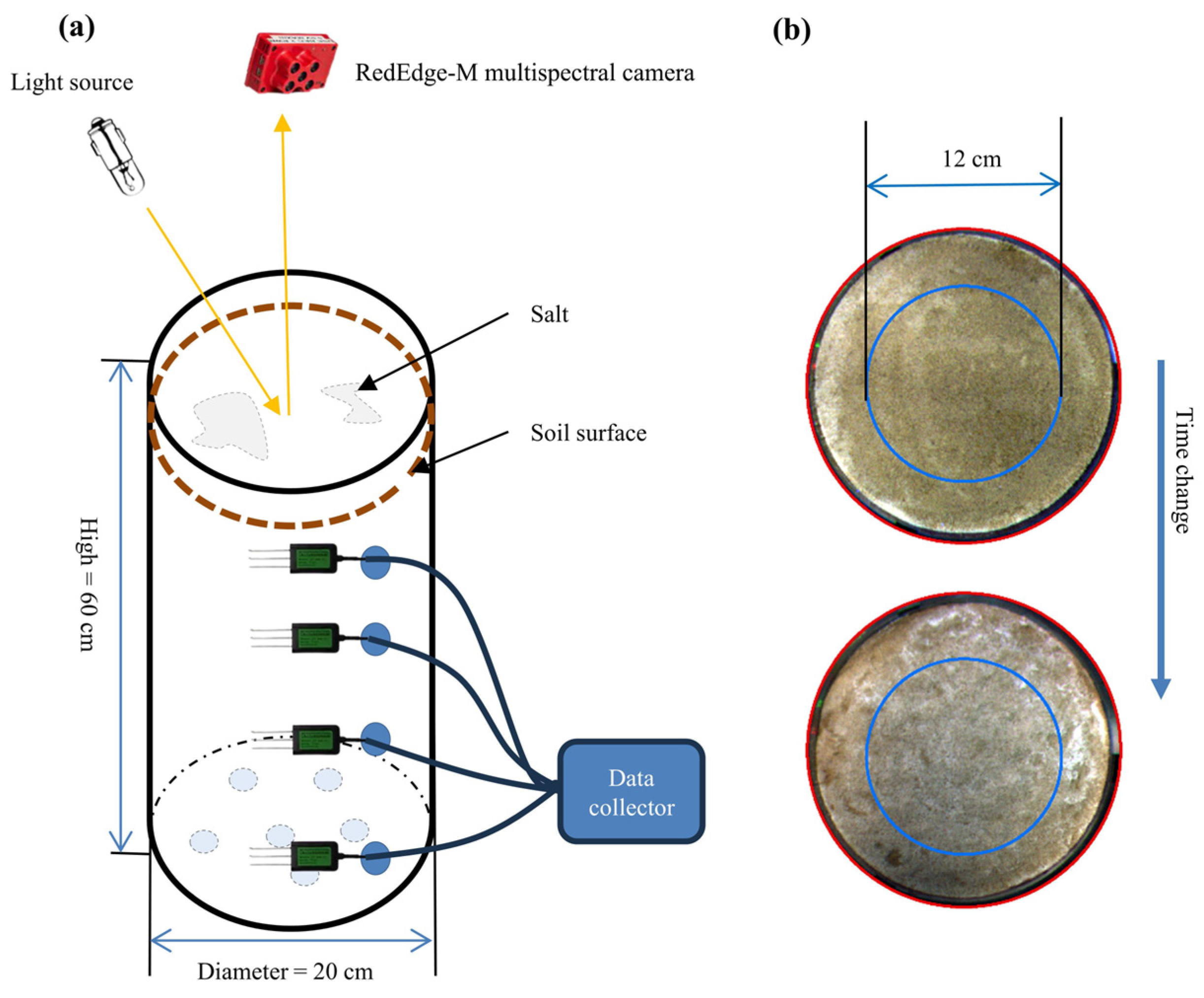
2.1. Design of the Experimental Setup for the Indoor Soil Column Experiment

According to the soil column experiment of Shokri-Kuehni et al. [25], as shown in Figure 1a, a plexiglas tube with a height of 60 cm and an outer diameter of 20 cm was used for this experiment. Figure 1b shows the precipitation deposition of soil salts on the surface over time. Small holes were made in the bottom of the soil column for drainage, and for installation of the soil water and salt monitoring instrument, 5 cm diameter holes were drilled laterally at 7 cm, 22 cm, 37 cm, and 52 cm from the upper edge of the plexiglas tube, named Soil layer-1, Soil layer-2, Soil layer-3, and Soil layer-4 in order of depth. Soil volumetric water content, bulk soil electrical conductivity (EC_b, us/cm), and temperature (°C) were obtained using a soil moisture monitoring instrument (FT-TS400, Shandong Fengtu IOT Technology Co., Ltd., Weifang, China). The soil moisture monitoring instrument was factory-calibrated and validated. Data were automatically collected every 5 min. Soil volumetric water content: range: 0–100%; accuracy: ±3%. Bulk soil electrical conductivity: range: 0–20,000 µS/cm; accuracy: ±3% (0–10,000 µS/cm), ±5% (10,000–20,000 µS/cm); resolution: 10 µS/cm (0–10,000 µS/cm), 50 µS/cm (10,000–20,000 µS/cm). Temperature: range: −40 to +125 °C; accuracy: ±0.5 °C; resolution: 0.1 °C. The experiment was designed with three soil columns, each filled and compacted with sandy soil of different water content and salinity gradients (see

Table 1. Initial water content and salinity of soil columns.

Soil Column	Layer Name	Initial Water Content (%)	Initial Salinity (μS/cm)
Soil column A	Soil layer-1	1.704	0.000
	Soil layer-2	1.280	0.000
	Soil layer-3	2.093	0.000
	Soil layer-4	1.160	0.000
Soil column B	Soil layer-1	9.020	260.000
	Soil layer-2	6.660	268.150
	Soil layer-3	2.800	143.000
	Soil layer-4	1.704	1.000
Soil column C	Soil layer-1	16.675	647.250
	Soil layer-2	11.255	390.750
	Soil layer-3	11.730	486.250
	Soil layer-4	15.490	561.500

for initial water content and salinity), with the upper surface 2 cm from the upper edge of the soil column. The salt we used is a mixture of sodium chloride and sodium sulfate. The milligram equivalent ratio of chloride to sulfate ions is 0.676056. The weight of the soil column was weighed below the column using an electronic scale (accuracy ±0.01 kg) for measuring evaporation, and the weight was weighed twice a day at regular intervals in the morning and evening. The laboratory was supplied with radiators, so there was little difference in temperature and humidity between day and night, with an average room air temperature of about 25.33 ± 0.83 °C and an average humidity of 22.24 ± 3.42% throughout the experiment. Soil texture was measured by a Malvern laser particle size analyzer (Mastersizer 3000; Malvern Panalytical, Malvern, UK) after pretreatment of soil column soil. The measured soil texture contained 0.47%, 4.38%, and 95.15% clay, silt, and sand, respectively, and the ring knife method measured a field capacity of 1.537 g/cm³, making the soil texture type homogeneous sandy (

Table 2. Soil physical properties.

Soil Type	Upper Cumulative Results (2 μm)	Results in the Interval (2, 50 μm)	Results in the Interval (50, 2000 μm)	Bottom Cumulative Result (2000 μm)	Specific Surface Area Result
	0.47	4.38	95.15	1 × 10−11	37.67

). Soil hydraulic parameters were measured using the centrifugal method (H-1400 pF centrifuge for soil, Kokusan Corporation, Kyoto, Japan); the soil moisture characteristic curve was fitted using the Pyswr module in Python 3.9 and the fitted curve is shown in Figure 2.

In order to obtain continuous soil spectral data during the experimental period, a Micasense RedEdge-M multispectral camera (RedEdge-M, MicaSense Inc., Seattle, WA, USA) was used to capture multispectral images of the soil surface with detailed spectral information shown in

Table 3. Micasense RedEdge-M camera band spectral information.

Band Number	Band Name	Center Wavelength (nm)	Bandwidth (nm)
Band 1	Blue band	475	20
Band 2	Green band	560	20
Band 3	Red band	668	10
Band 4	Near-infrared band	840	40
Band 5	RedEdge band	717	10

, referring to the study of Shi et al. [27]. The camera was fixed at a height of 50 cm from the soil surface using a bracket and the camera was used in the manual mode, with the angle of capture being perpendicular to the soil surface. A halogen lamp was used to provide a light source to simulate sunlight; the angle of the light source was 30° from the shooting angle, and the light source was 45 cm from the center of the soil surface. At the beginning of the experiment, the soil surface was photographed under darkroom conditions, and the initial image was taken once before the addition of saline water, and then hourly due to the rapid changes in the soil surface in the early part of the experiment. Because the evaporation process slowed down significantly after about 2 days, the soil surface changed more slowly and was photographed about once every 2 or 4 h, and was not photographed at night. The saline water addition experiments were conducted three times, with the first experiment lasting 60 h and the second and third experiments totaling 80 h. In the first experiment, the water addition was set at 1 mm of precipitation or irrigation, and the salinity was 1 g/L. In the second and third experiments, the water addition was set at 2 mm and 4 mm, and the salinity was 2 g/L. The soil surface was not changed at night.

2.2. Multispectral Camera Data Processing

The RedEdge-M multispectral camera utilizes a multi-lens imaging mechanism in a multi-camera imaging system. The RedEdge-M multispectral camera contains five independent imaging lenses, each of which performs imaging independently and stores the results as separate image files. Therefore, when combining the images of different bands, there will be an obvious misalignment offset phenomenon, which requires image alignment work.

Virtual imaging is a method of re-projecting each lens onto an ideal virtual image by utilizing the positional relationship between them [28,29]. When processing RedEdge-M images, the use of a virtual imaging technique can easily realize the band alignment without the need to know the outer azimuthal elements of the image and the Digital Elevation Model (DEM) of the survey area in advance, but only the average relative speed at the time of aerial photography. Therefore, in this study, we adopt the virtual imaging technique as an alignment method for the images between different bands of the RedEdge-M camera. The general adoption of the virtual imaging method realizes the waveband alignment with sub-image-element accuracy, and the alignment accuracy is better than 0.3 image pixels.

2.3. Calculation of the Salinity Spectral Index

In order to assess the relationship between soil water content and salinity on the surface of the soil column and the changes in remotely sensed salinity indices, one vegetation index and ten salinity indices were calculated (

Table 4. Spectral indices used in the experiment and calculation formulae.

Index Names	Calculation Equation	Reference
NDVI	$(NIR-Red)/(NIR+Red)$	[30]
SI	${\left(Blue+Red\right)}^{0.5}$	[31]
SI1	${\left({Green}^2\times {Red}^2\right)}^{0.5}$
SI2	${\left({Green}^2+{Red}^2+{NIR}^2\right)}^{0.5}$	[32]
SI3	${\left({Green}^2+{Red}^2\right)}^{0.5}$
S1	$Blue/Red$
S2	$(Blue-Red)/(Blue+Red)$	[33]
S3	$Green\times Red/Blue$
S4	${\left(Blue\times Red\right)}^{0.5}$
S5	$Blue\times Red/Gree$	[34]
S6	$Red\times NIR/Green$

), and all of these remotely sensed indices were shown to be significantly correlated with soil surface salinity. In general, the vegetation index showed a moderately significant negative correlation with soil salinity, while the salinity index related to soil background showed a moderately significant positive correlation with soil salinity.

3. Results

3.1. Variation in Band Reflectance on the Surface of Soil Column

To compare the change in reflectance of different bands on the surface of the soil column with time after water addition, the first multiband image acquired after water addition and the last multiband image at the end period of the experiment were subjected to pixel counting, and the counting results are shown in box plots (Figure 3). The overall results show an increasing trend in band reflectance with increasing band wavelength. A comparison of the statistical characteristics of the first and the last images after water addition reveals that the mean, median, and quartile of the image element statistics of the last image have increased reflectance in all bands compared to the first image. Among them, the exception is soil column A of the first set of experiments, which may be due to too little precipitated salts. Within the same set of experiments, the reflectance increase for the three soil columns will be arranged in accordance with the gradient of initial salinity conductivity, i.e., it satisfies soil column C > soil column B > soil column A, which suggests that the initial soil salinity will affect the process of the increase in soil surface salinity reflectance.

3.2. Characteristics of Water Content Change in Soil Column Layers

Figure 4 shows the process of soil water content change in the stratified layers of the three soil columns during the three sets of experiments. The experimental results show that in the first set of experiments, the soil water content of the first soil layer in the three soil columns changed the most, in which the range of change was sorted as soil column C > soil column B > soil column A. This result was mainly controlled by the initial water content. Soil column A was in a dry state and the initial water content was very low; the first set of experiments added water to infiltrate the surface soil and for water infiltration into the second layer. The water content of the surface layer of soil column B showed a peak after adding water, but the water content did not exceed 20%, and the water content of the second layer gradually increased, which was controlled by water infiltration. The water content in the surface layer of soil column C also showed a peak, but the variation was larger than that in soil columns A and B, with a value of about 65%, and the water content in its second layer also showed a slow increase in the phenomenon, but it did not exceed 20% and then leveled off. In the second set of experiments, the overall change in the three soil columns also satisfies the order of soil column C > soil column B > soil column A. In the three soil columns, the water content in the surface layer and the second layer increased rapidly at first and then decreased slowly, which was mainly controlled by water infiltration. Among them, the peak of the second layer in soil column B was larger than the peak of the first layer, which might be caused by the infiltration of water from the upper layer together with the added water. The third layer of soil column C experienced a gradual increase in water content after a period of plateauing, which was also caused by the infiltration of water from the upper layer. In the third set of experiments, the surface layer and the third layer satisfied the same pattern. However, in soil columns B and C, the water content of the fourth soil layer increased and then leveled off, with soil column B leveling off at about 60% of the water content, while the fourth layer in soil column C was saturated.

Overall, the water movement process in the three sets of experiments was mainly controlled by the initial water content and water infiltration process. When the soil water content is not saturated, there will be a peak and then a slow decline phenomenon, and the soil water will eventually accumulate in a certain layer.

3.3. Characteristics of Conductivity Change in Soil Column Layers

The EC_b change process of stratified soil in the different soil columns of the three experimental groups in this study is shown in Figure 5. The results showed that the EC_b change rule of stratified soil was similar to that of soil moisture transport. In the first group of experiments, the EC_b of the surface layer of soil column A showed the change rule of increasing and then slowly decreasing, and the surface layer of soil column B and soil column C also showed a peak and then slowly decreased, but the second layer of soil column C showed a slow increase and then leveled off, indicating that the second layer of soil column C showed the phenomenon of salt accumulation. The peak fluctuations for soil column C were in the order of amplitude of soil column C > soil column B > soil column A, which was mainly controlled by the initial water content and salinity of the soil. In the second set of experiments, the surface layer also showed the phenomenon of peak increase and then decrease, and the peak fluctuations were also in the order of magnitude of soil column C > soil column B > soil column A. The EC_b in the third layer of soil column B and soil column C showed the phenomenon of slow increase, which was also controlled by the initial water content and salinity. In soil column B, the EC_b in the second layer was larger than that in the first layer after the EC_b leveled off, which was mainly caused by the water washing the surface soil and bringing salts into the second layer. In the third set of experiments, the surface layer, the second layer, and the third layer all showed the phenomenon of increasing peaks and then decreasing peaks, and the peak fluctuations were in the order of magnitude of soil column C > soil column B > soil column A. Among them, the values of the third layer of EC_b were larger than those of the first layer and the second layer after leveling off, which was also caused by the water washing of the surface soil and bringing salts into the second layer. In the fourth layer of soil columns B and C, the EC_b increased slowly and then leveled off, suggesting that soil salts accumulated at this location after water washing.

Overall, the salt movement process in the three sets of experiments was mainly controlled by the combination of initial water content and salt content and the water infiltration process. After each water addition experiment, there was a peak and then a slow decline phenomenon, indicating the washing effect of water on the soil salts, and the soil salts eventually accumulated in a layer due to the water movement. This process fully demonstrates the water–salt transport law of “salt moves together with water, and when water evaporates, salt is retained in the soil weight”.

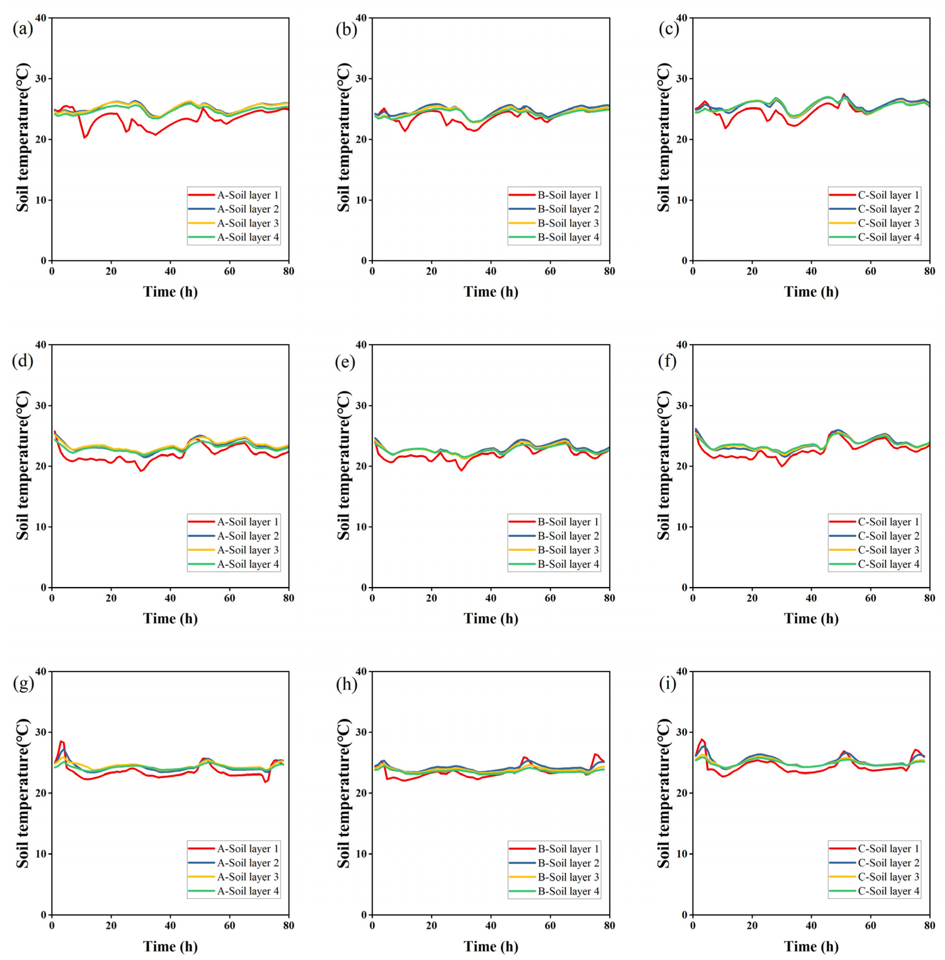
3.4. Temperature Changes in Soil Column Layers

The soil sensors simultaneously acquired the temperature changes in the soil column layer, and the results are shown in Figure 6. Overall, the temperature results of the soil column layering in different groups of experiments did not change much during the experimental period, showing fluctuation, and the process of change was consistent in each layer. Among them, the largest fluctuation was in the topsoil layer, and the temperature was lower than the temperature at the bottom of the soil column overall. This is different from the natural state of the soil profile temperature from top to bottom according to the decreasing law; the reason may be that the natural state of the deep soil cannot be directly exposed to solar radiation, and the experimental environment in which the soil column is located cannot completely simulate field conditions. However, it is not difficult to see that the temperature in different soil layers has little effect on the water and salt transport process in the soil.

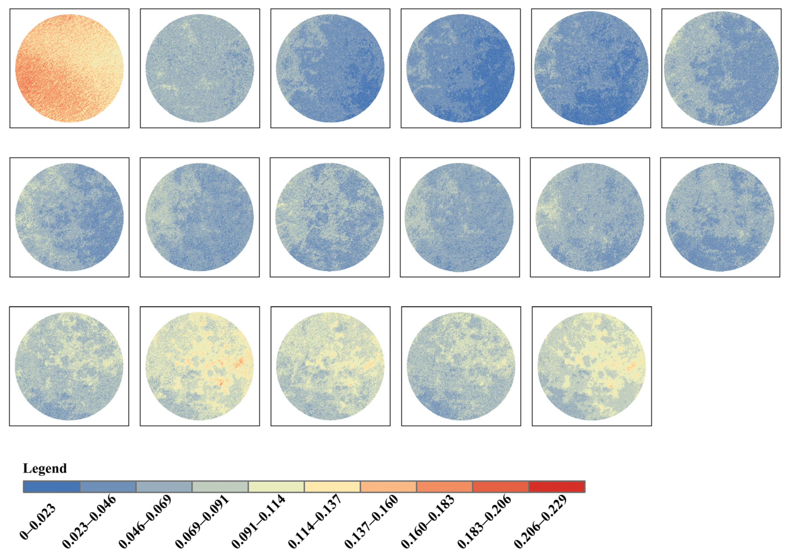
3.5. Characteristics of Changes in the Surface Salinity Index of Soil Columns

In order to investigate the characteristics of the variation in the surface salinity index of the soil columns, the mean value of the soil surface salinity index of each group of experiments was nonlinearly fitted to time. The fitting results showed that most of the soil surface salinity index mean values versus time satisfy the Freundlich equation:

$$Salinityindex=a{T}^{{bT}^{-c}}$$

where Salinity index is various salinity indices; T is time; and a, b, and c are constant covariates.

The fitting results that were not significant and not converged were excluded, and all the results were averaged according to different remote sensing indices; the results are shown in

Table 5. Mean accuracy of the model fitted to the salinity index vs. time.

Salinity Index	R2	RMSE
NDVI	0.274	0.019
S1	0.451	0.010
S2	0.469	0.017
S3	0.624	0.123
S4	0.726	0.011
S5	0.734	0.009
S6	0.704	0.115
SI	0.719	0.020
SI1	0.730	0.057
SI2	0.729	0.032
SI3	0.702	0.038

. The results showed that the vegetation index NDVI had the lowest fitting accuracy, with an R² of 0.274 and an RMSE of 0.019. This was because there was no vegetation information on the surface of the bare soil of the soil column, and it would be less accurate to use the vegetation index to indicate the change in salinity on the bare soil. The highest fitting accuracy was found in salinity index S5 with an R² of 0.734 and RMSE of 0.009. Overall, most of the salinity indices had high fitting accuracy and significant fitting models. The salinity indices with lower fitting accuracies were salinity indices S1 and S2, which may indicate that salinity indices S1 and S2 are less applicable in monitoring soil salinity changes. All other fitting results are presented in the Supplementary Materials.

In order to clearly demonstrate the characteristics of the salinity index with time, salinity index S5 with the highest fitting accuracy is displayed in Figure 7, and the other various indices are shown in Figure 7 in relation to time; the fitting accuracies are shown in the Supplementary Materials. The results showed that salinity index S5 had a high starting value at the beginning of each group of experiments, decreased instantly after water addition, and then increased slowly with time. This process indicates that the effect of water addition on soil surface salinity is in accordance with the basic water–salt transport law of “salt moves together with water, and when water evaporates, salt is retained in the soil weight”. As for the other spectral indices in the annex, except for the NDVI, which has no obvious change characteristics, all the other salinity indices conform to the rule of change.

In order to clearly show the change process of salinity index on the soil surface, the change process of S5 of soil column A in the first group of experiments is shown in Figure 8, and the change process of S5 on the surface of soil columns of other experiments is similar to that of Figure 8, and therefore it is put in the annex. The results show that the process of salinity index S5’s changes with time for soil column A in the first set of experiments is consistent with the above process. The explanation of the process of salinity index S5’s change on the surface of the soil column can be that in the initial state (original analyzed without salt or analyzed with salt), S5 decreased instantly after the addition of brine, and after that, under evaporation, salt precipitated to form salt crystals on the surface of the soil, which led to the process of S5 showing a decrease and then a slow increase. The results also showed that there was heterogeneity in the salinity changes in the surface space of the soil columns, presenting inhomogeneous variations, especially in the later stages of the experiment, when the values of salinity index S5 on the surface of the soil columns were in the range of 0.069 to 0.229. This agrees with the manifestation of a strong heterogeneity of the soil salinity in the space in the natural state.

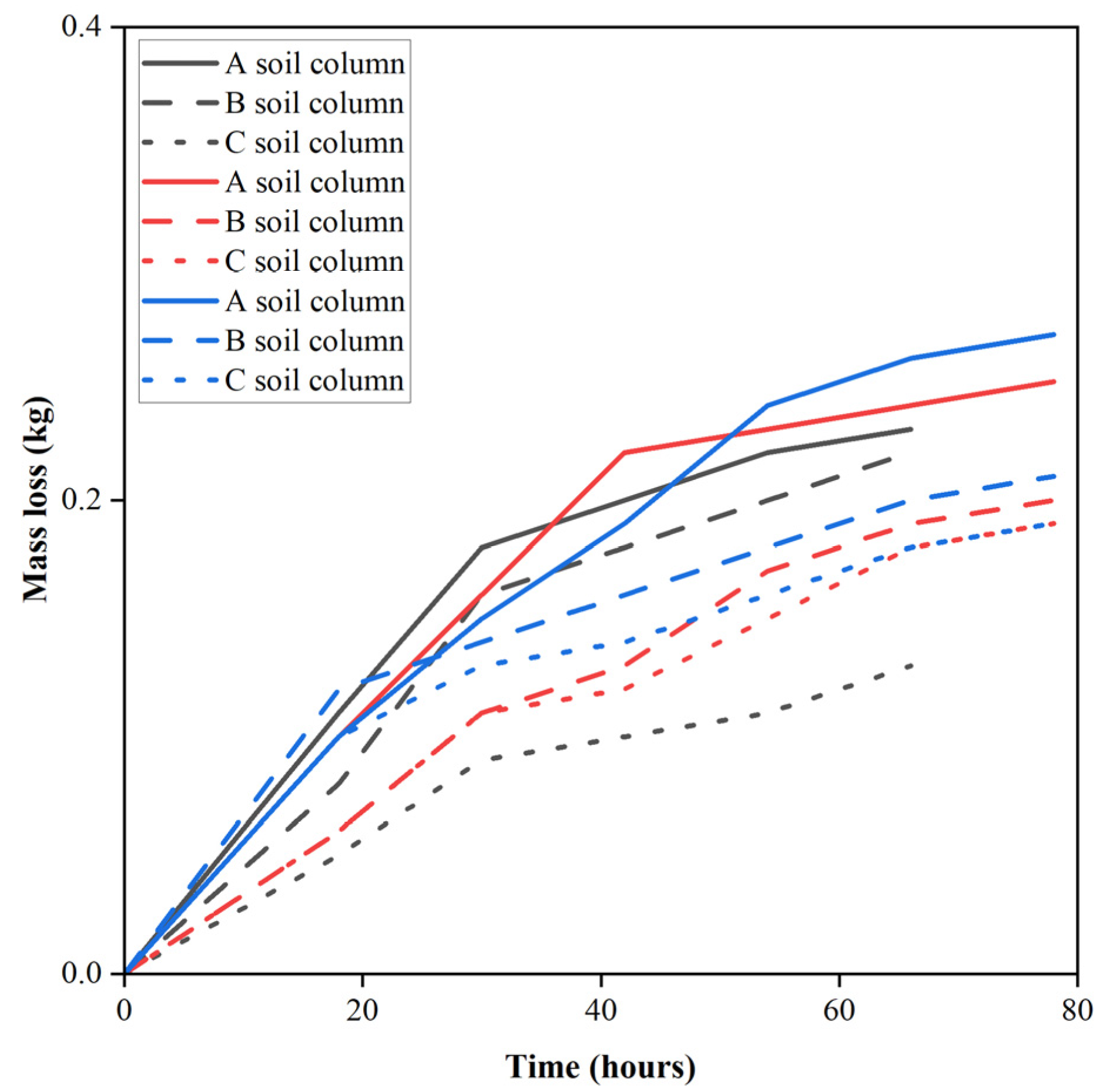
3.6. Accumulation of Mass Loss in the Soil Column during the Experiment

The process of salt accumulation on the soil surface is related to the evaporation process. The relationship between the evaporation process and salt accumulation was investigated by weighing the mass of each soil column in the three groups of experiments during the experimental period to obtain the cumulative mass loss of the soil columns, and the results are shown in Figure 9. The results show that the process of mass loss accumulation for each soil column in each group of experiments was similar, and the overall process of mass loss accumulation increased first and then the process of increase slowed down, i.e., the process of mass loss accumulation showed a logarithmic pattern. A comparison of the different groups of experiments shows that soil column C has the smallest cumulative magnitude in mass loss accumulation, while soil column A has the largest cumulative magnitude in mass loss accumulation. The reasons may consist of two parts, firstly, the initial water content of each soil column is different, which leads to a difference in mass loss accumulation in the evaporation process; secondly, the salt content of soil column C is the highest among the soil columns, and after the salt precipitates out and crystallizes on the surface of the soil, the salt crust or the soil crust has an inhibitory effect on the evaporation process of the soil columns.

4. Discussion

4.1. Changes in Soil Spectral Reflectance

In this study, a multispectral camera was used to photograph the soil surface, which allowed us to investigate the characteristics of the change in spectral reflectance of the soil surface, and the results showed that the spectral reflectance of each band of the image at the end of the experiment was higher than that of the band at the beginning of the experiment after the addition of water during the test period. Many studies using remote sensing to monitor surface salinity have also pointed out that the spectral reflectance of images of high-salinity soils is higher than that of low-salinity soils [35,36,37]. Previous studies, however, mostly focused on the same scene image and explored the spatial variation in salinity, while it is difficult to explain the difference in spectral reflectance of the same site over time [19]. The reason for this is mainly water–salt transport, in which water accumulates and precipitates salts on the surface by capillary forces and evaporation, resulting in an increase in spectral reflectance in the band [38]. Similarly, it is caused by changes in the matric potential difference of moisture, which cause moisture to move from the wet to the dry zone, leading to salt accumulation and precipitation on the surface and resulting in an increase in the spectral reflectance in the band [39]. Different initial salt states of the soil column caused different results, so it showed that the initial state of the soil affects the salt accumulation process. Interpreting the addition of water in the experiment as precipitation or irrigation, the results of this study also showed that the spectral reflectance of saline soils at the same site was affected by precipitation or irrigation. Over-irrigation can cause soil salinization and reduce water use efficiency [40]. Soil surface spectral reflectance is affected by many factors, such as salt type, soil type, light conditions, and salt crust conditions. The available indoor spectral measurements are mostly hyperspectral, and in general the spectral reflectance increases with increasing salinity and is strongly influenced by the type of salinity [41,42]. The effect of salt type is greater than that of soil texture, especially for some hygroscopic salts (MgCl₂ and CaCl₂). Spectral measurements of saline soils under natural light sources can distinguish between crusted and non-crusted surfaces and help assess the extent of crust development [43]. Meanwhile, some scholars pointed out that the height of the soil column affects the moisture and salt content in the soil column, which indirectly affects the measurement of laboratory soil spectra [26]. Soil temperature is regarded by many scholars as an important environmental indicator for soil salinity monitoring, but the results of this study show that soil temperature has little effect on the process of spectral changes on the surface of soil columns.

4.2. Relationship between Soil Column Water and Salt Transport Laws and Surface Soil Spectral Indices

The results of water and salt transport in this study fully reflected the basic water and salt transport law of “salt moves together with water, and when water evaporates, salt is retained in the soil weight”, but it is not clear whether some commonly used spectral indices are consistent with this law and its mechanism. When remote sensing is used to monitor soil salinity, the purpose of constructing the soil salinity index is to make the soil surface salinity information easier to distinguish, differentiate the surface salinity from other features, and to make the salinity gradient easier to represent. Some scholars analyzed the relationship between surface spectral reflectance data and the salt content of subsurface soils (5 cm and 15 cm) by using the structural equation modeling (SEM) method, and the results pointed out that there were significant correlations between soil surface spectral reflectance and subsurface soil salinity, as well as between different types of multispectral data (e.g., Landsat data) and subsurface soil salinity [44].

Considering the complexity of the salinization process, it is very difficult to achieve accurate detection in the early stages of occurrence. Often, high concentrations of salt affect some physical and chemical properties of the soil, and these properties may be detected even if there is no salt weathering on the soil surface. This is especially the case when no salt crust is formed on the surface; however, it is difficult to meet the application requirements for the salinization process and the deep salt accumulation phenomenon using only remote sensing techniques. One idea to solve this problem is to couple numerical simulation with remote sensing techniques, but first the mapping relationship between soil surface spectra and water–salt transport needs to be understood. As the results of this study show, the soil salinity index on the surface of the soil column decreases rapidly after the addition of water and shows a slow increase process with the evaporation process. In the natural state, saline soils affected by precipitation or irrigation will produce changes in the soil salinity index, which may affect the accuracy of large-scale remote sensing to monitor soil salinization [45].

4.3. Limitations and Future

Analyzing the experimental process and results, the limitations of this work are mainly reflected in three points: The first is that the experimental process cannot accurately obtain the salinity of the pore water, which has been difficult to accurately obtain with the current technical means. The second point is that the work did not achieve the process of coupling remote sensing and physical modeling to model the monitoring of soil water and salt changes. The third point is the difference between indoor and outdoor environments, for example, the results of indoor experiments cannot be matched with outdoor results due to the fact that indoor heating leads to a very weak effect of temperature changes, and similarly indoors is very weakly affected by wind. Despite the limitations of this study, these limitations did not affect the conclusions of this work. In future work, it is necessary to construct a model and framework method for monitoring soil water salinity changes by coupling remote sensing and physical modeling, and this study has provided some theoretical basis for this direction. Our experiments mainly used sandy soils, and in the next research work we need to investigate the use of other types of soils such as clay and loam and compare their saline properties and behavioral results with the current results.

5. Conclusions

In this study, we used an indoor soil column experiment, an unmanned aerial vehicle multispectral sensor camera, and a soil moisture sensor to study the water and salt transport process in the soil column under different water addition conditions, investigate the relationship between the soil water and salt transport process and the spectral reflectance of the image on the soil surface, and analyze the relationship between the water and salt transport process and the salinity index of the soil surface. The observation results of the soil column showed that the soil water and salt transport process conformed to the basic transport law of “salt moves together with water, and when water evaporates, salt is retained in the soil weight”, and water and salt would accumulate at the bottom of the soil column in the late stage of the experiment. The phenomenon of salt accumulation affects the image reflectance results. With the precipitation and deposition of salt, the reflectance of the soil surface increases, and the soil temperature does not show any effect on the spectra, while the salinity index decreases instantly after the addition of water and then shows a slow increasing trend. The innovation of this experiment is the use of an unmanned aerial vehicle multispectral sensor camera to calculate different salinity indices, which is able to obtain finer soil salinity information and improve the soil water and salt surface observation technique during the experiment. The results of our work are more applicable to the process of water and salt transport changes in an arid zone. This work can provide a theoretical basis and reference for constructing a coupled model of remote sensing observation technology and a soil physical model for soil water salinity monitoring.

References

1. Wu, H.; Guo, B.; Fan, J.; Yang, F.; Han, B.; Wei, C.; Lu, Y.; Zang, W.; Zhen, X.; Meng, C. A novel remote sensing ecological vulnerability index on large scale: A case study of the China-Pakistan Economic Corridor region. Ecol. Indic. 2021, 129, 107955. [Google Scholar] [CrossRef]
2. Vineis, P.; Khan, A. Climate Change–Induced Salinity Threatens Health. Science 2012, 338, 1028–1029. [Google Scholar] [CrossRef] [PubMed]
3. Prăvălie, R. Exploring the multiple land degradation pathways across the planet. Earth-Sci. Rev. 2021, 220, 103689. [Google Scholar] [CrossRef]
4. Sahab, S.; Suhani, I.; Srivastava, V.; Chauhan, P.S.; Singh, R.P.; Prasad, V. Potential risk assessment of soil salinity to agroecosystem sustainability: Current status and management strategies. Sci. Total Environ. 2021, 764, 144164. [Google Scholar] [CrossRef]
5. McNeill, J.R.; Winiwarter, V. Breaking the Sod: Humankind, History, and Soil. Science 2004, 304, 1627–1629. [Google Scholar] [CrossRef] [PubMed]
6. Godfray, H.C.J.; Beddington, J.R.; Crute, I.R.; Haddad, L.; Lawrence, D.; Muir, J.F.; Pretty, J.; Robinson, S.; Thomas, S.M.; Toulmin, C. Food Security: The Challenge of Feeding 9 Billion People. Science 2010, 327, 812–818. [Google Scholar] [CrossRef]
7. Zhao, Q.; Bai, J.; Zhang, G.; Jia, J.; Wang, W.; Wang, X. Effects of water and salinity regulation measures on soil carbon sequestration in coastal wetlands of the Yellow River Delta. Geoderma 2018, 319, 219–229. [Google Scholar] [CrossRef]
8. Aimen, A.; Kuandykova, G.; Suleimenova, I.; Tashmukhamedov, F.; Demeuova, G.; Anarova, G.; Aimenova, S.; Moldasheva, A.J.I.J.O.E.; Sciences, E. Environmental evaluation of water salt exchange process in soil degradation in the arid zone. Int. J. Ecosyst. Ecol. Sci. 2022, 12, 33. [Google Scholar] [CrossRef]
9. Daliakopoulos, I.N.; Tsanis, I.K.; Koutroulis, A.; Kourgialas, N.N.; Varouchakis, A.E.; Karatzas, G.P.; Ritsema, C.J. The threat of soil salinity: A European scale review. Sci. Total Environ. 2016, 573, 727–739. [Google Scholar] [CrossRef]
10. Abrol, I.; Yadav, J.S.P.; Massoud, F. Salt-Affected Soils and Their Management; Food & Agriculture Organization: Rome, Italy, 1988; Volume 39. [Google Scholar]
11. Wu, W.; Al-Shafie, W.M.; Mhaimeed, A.S.; Ziadat, F.; Nangia, V.; Payne, W.B. Soil Salinity Mapping by Multiscale Remote Sensing in Mesopotamia, Iraq. IEEE J. Sel. Top. Appl. Earth Obs. Remote Sens. 2014, 7, 4442–4452. [Google Scholar] [CrossRef]
12. Hassani, A.; Azapagic, A.; Shokri, N. Global predictions of primary soil salinization under changing climate in the 21st century. Nat. Commun. 2021, 12, 6663. [Google Scholar] [CrossRef] [PubMed]
13. Lhissoui, R.; Harti, A.E.; Chokmani, K. Mapping soil salinity in irrigated land using optical remote sensing data. Eurasian J. Soil Sci. 2014, 3, 82–88. [Google Scholar] [CrossRef]
14. Chaaou, A.; Chikhaoui, M.; Naimi, M.; Miad, A.K.E.; Bokoye, A.I.; Ennasr, M.S.; Harche, S.E. Potential of land degradation index for soil salinity mapping in irrigated agricultural land in a semi-arid region using Landsat-OLI and Sentinel-MSI data. Environ. Monit. Assess. 2024, 196, 843. [Google Scholar] [CrossRef] [PubMed]
15. Metternicht, G.I.; Zinck, J.A. Remote sensing of soil salinity: Potentials and constraints. Remote Sens. Environ. 2003, 85, 1–20. [Google Scholar] [CrossRef]
16. Sahbeni, G.; Ngabire, M.; Musyimi, P.K.; Székely, B. Challenges and Opportunities in Remote Sensing for Soil Salinization Mapping and Monitoring: A Review. Remote Sens. 2023, 15, 2540. [Google Scholar] [CrossRef]
17. Guo, B.; Zang, W.; Luo, W.; Wen, Y.; Yang, F.; Han, B.; Fan, Y.; Chen, X.; Qi, Z.; Wang, Z.; et al. Detection model of soil salinization information in the Yellow River Delta based on feature space models with typical surface parameters derived from Landsat8 OLI image. Geomat. Nat. Hazards Risk 2020, 11, 288–300. [Google Scholar] [CrossRef]
18. Miller, B.A.; Lee Burras, C. Comparison of Surficial Geology Maps Based on Soil Survey and in Depth Geological Survey. Soil Horiz. 2015, 56, 1–12. [Google Scholar] [CrossRef]
19. Ben-Dor, E.; Chabrillat, S.; Demattê, J.A.M.; Taylor, G.R.; Hill, J.; Whiting, M.L.; Sommer, S. Using Imaging Spectroscopy to study soil properties. Remote Sens. Environ. 2009, 113, S38–S55. [Google Scholar] [CrossRef]
20. Farifteh, J.; Farshad, A.; George, R.J. Assessing salt-affected soils using remote sensing, solute modelling, and geophysics. Geoderma 2006, 130, 191–206. [Google Scholar] [CrossRef]
21. Han, M.; Zhao, C.; Šimůnek, J.; Feng, G. Evaluating the impact of groundwater on cotton growth and root zone water balance using Hydrus-1D coupled with a crop growth model. Agric. Water Manag. 2015, 160, 64–75. [Google Scholar] [CrossRef]
22. Yang, T.; Šimůnek, J.; Mo, M.; McCullough-Sanden, B.; Shahrokhnia, H.; Cherchian, S.; Wu, L. Assessing salinity leaching efficiency in three soils by the HYDRUS-1D and -2D simulations. Soil Tillage Res. 2019, 194, 104342. [Google Scholar] [CrossRef]
23. Ramos, T.B.; Darouich, H.; Oliveira, A.R.; Farzamian, M.; Monteiro, T.; Castanheira, N.; Paz, A.; Alexandre, C.; Gonçalves, M.C.; Pereira, L.S. Water use, soil water balance and soil salinization risks of Mediterranean tree orchards in southern Portugal under current climate variability: Issues for salinity control and irrigation management. Agric. Water Manag. 2023, 283, 108319. [Google Scholar] [CrossRef]
24. Han, L.; Ding, J.; Ge, X.; He, B.; Wang, J.; Xie, B.; Zhang, Z. Using spatiotemporal fusion algorithms to fill in potentially absent satellite images for calculating soil salinity: A feasibility study. Int. J. Appl. Earth Obs. Geoinf. 2022, 111, 102839. [Google Scholar] [CrossRef]
25. Shokri-Kuehni, S.M.S.; Norouzi Rad, M.; Webb, C.; Shokri, N. Impact of type of salt and ambient conditions on saline water evaporation from porous media. Adv. Water Resour. 2017, 105, 154–161. [Google Scholar] [CrossRef]
26. Xu, L.; Wang, Z.-c.; Nyongesah, J.M. Soil Column Sample Height Influences Soil Spectral Reflectance in Laboratory Experiment. J. Indian Soc. Remote Sens. 2019, 47, 1187–1196. [Google Scholar] [CrossRef]
27. Shi, T.; Cui, L.; Wang, J.; Fei, T.; Chen, Y.; Wu, G. Comparison of multivariate methods for estimating soil total nitrogen with visible/near-infrared spectroscopy. Plant Soil 2013, 366, 363–375. [Google Scholar] [CrossRef]
28. Jhan, J.-P.; Rau, J.-Y.; Huang, C.-Y. Band-to-band registration and ortho-rectification of multilens/multispectral imagery: A case study of MiniMCA-12 acquired by a fixed-wing UAS. ISPRS J. Photogramm. Remote Sens. 2016, 114, 66–77. [Google Scholar] [CrossRef]
29. Jhan, J.-P.; Rau, J.-Y.; Haala, N. Robust and adaptive band-to-band image transform of UAS miniature multi-lens multispectral camera. ISPRS J. Photogramm. Remote Sens. 2018, 137, 47–60. [Google Scholar] [CrossRef]
30. Deering, D.; Haas, R. Using Landsat digital data for estimating green biomass. In Proceedings of the Ann. Meeting of the Soc. for Range Management Symp. on Rangeland Remote Sensing, Portland, OR, USA, 17 February 1980; Available online: http://ntrs.nasa.gov/archive/nasa/casi.ntrs.nasa.gov/19800024311.pdf (accessed on 25 January 2015).
31. Khan, N.M.; Rastoskuev, V.V.; Sato, Y.; Shiozawa, S. Assessment of hydrosaline land degradation by using a simple approach of remote sensing indicators. Agric. Water Manag. 2005, 77, 96–109. [Google Scholar] [CrossRef]
32. Douaoui, A.E.K.; Nicolas, H.; Walter, C. Detecting salinity hazards within a semiarid context by means of combining soil and remote-sensing data. Geoderma 2006, 134, 217–230. [Google Scholar] [CrossRef]
33. Abbas, A.; Khan, S. Using remote sensing techniques for appraisal of irrigated soil salinity. In Proceedings of the International Congress on Modelling and Simulation (MODSIM), Christchurch, New Zealand, 10–13 December 2007; Modelling and Simulation Society of Australia and New Zealand: Canberra, Australia, 2007; pp. 2632–2638. [Google Scholar]
34. Allbed, A.; Kumar, L.; Aldakheel, Y.Y. Assessing soil salinity using soil salinity and vegetation indices derived from IKONOS high-spatial resolution imageries: Applications in a date palm dominated region. Geoderma 2014, 230–231, 1–8. [Google Scholar] [CrossRef]
35. Fan, X.; Liu, Y.; Tao, J.; Weng, Y. Soil Salinity Retrieval from Advanced Multi-Spectral Sensor with Partial Least Square Regression. Remote Sens. 2015, 7, 488–511. [Google Scholar] [CrossRef]
36. Abuelgasim, A.; Ammad, R. Mapping soil salinity in arid and semi-arid regions using Landsat 8 OLI satellite data. Remote Sens. Appl. Soc. Environ. 2019, 13, 415–425. [Google Scholar] [CrossRef]
37. Masoud, A.A. Predicting salt abundance in slightly saline soils from Landsat ETM+ imagery using Spectral Mixture Analysis and soil spectrometry. Geoderma 2014, 217–218, 45–56. [Google Scholar] [CrossRef]
38. Xing, X.; Li, X.; Ma, X. Capillary rise and saliferous groundwater evaporation: Effects of various solutes and concentrations. Hydrol. Res. 2019, 50, 517–525. [Google Scholar] [CrossRef]
39. Hu, S.; Zhang, C.; Lu, N. Quantifying Coupling Effects between Soil Matric Potential and Osmotic Potential. Water Resour. Res. 2023, 59, e2022WR033779. [Google Scholar] [CrossRef]
40. Qin, S.; Ding, J.; Ge, X.; Wang, J.; Wang, R.; Zou, J.; Tan, J.; Han, L. Spatio-Temporal Changes in Water Use Efficiency and Its Driving Factors in Central Asia (2001–2021). Remote Sens. 2023, 15, 767. [Google Scholar] [CrossRef]
41. Farifteh, J.; van der Meer, F.; van der Meijde, M.; Atzberger, C. Spectral characteristics of salt-affected soils: A laboratory experiment. Geoderma 2008, 145, 196–206. [Google Scholar] [CrossRef]
42. Farifteh, J.; van der Meer, F.; Carranza, E.J.M. Similarity measures for spectral discrimination of salt-affected soils. Int. J. Remote Sens. 2007, 28, 5273–5293. [Google Scholar] [CrossRef]
43. Eshel, G.; Levy, G.J.; Singer, M.J. Spectral Reflectance Properties of Crusted Soils under Solar Illumination. Soil Sci. Soc. Am. J. 2004, 68, 1982–1991. [Google Scholar] [CrossRef]
44. Liu, Y.; Pan, X.; Wang, C.; Li, Y.; Shi, R. Can subsurface soil salinity be predicted from surface spectral information?—From the perspective of structural equation modelling. Biosyst. Eng. 2016, 152, 138–147. [Google Scholar] [CrossRef]
45. Han, L.; Ding, J.; Zhang, J.; Chen, P.; Wang, J.; Wang, Y.; Wang, J.; Ge, X.; Zhang, Z. Precipitation events determine the spatiotemporal distribution of playa surface salinity in arid regions: Evidence from satellite data fused via the enhanced spatial and temporal adaptive reflectance fusion model. Catena 2021, 206, 105546. [Google Scholar] [CrossRef]
Figure 1. Schematic diagram of the indoor soil column experimental setup. (a) shows a schematic diagram of the installation setup of the soil column dimensions, light source, camera, and soil sensor. (b) shows a true-color image of the soil surface as it changes over time and soil salts crystallize and precipitate.
Remotesensing 16 03421 g001
Figure 2. Characteristic soil moisture profiles of soil samples from soil columns measured by centrifugation.
Remotesensing 16 03421 g002
Figure 3. Comparison results of initial and end surface reflectance of three soil column experiments in three groups of experiments, where (ac) are the first set of experiments, (df) are the second set of experiments, and (gi) are the third set of experiments.
Remotesensing 16 03421 g003
Figure 4. Results of soil moisture content of different soil layers during the experiments of three soil columns in three groups of experiments, where (ac) is the first set of experiments, (df) is the second set of experiments, and (gi) is the third set of experiments.
Remotesensing 16 03421 g004
Figure 5. Soil conductivity results for different soil layers during the three soil column experiments in the three groups of experiments, where (ac) is the first set of experiments, (df) is the second set of experiments, and (gi) is the third set of experiments.
Remotesensing 16 03421 g005
Figure 6. Soil temperature results for different soil layers during the three soil column experiments in the three groups of experiments, where (ac) is the first set of experiments, (df) is the second set of experiments, and (gi) is the third set of experiments.
Remotesensing 16 03421 g006
Figure 7. Results of salinity index S5 with time for each soil column in the three sets of experiments. (ac) are for the first, second, and third experiments, respectively.
Remotesensing 16 03421 g007
Figure 8. The change process of salinity index S5 of soil column A in the first experiment.
Remotesensing 16 03421 g008
Figure 9. Cumulative mass loss of each soil column in three groups of experiments. The line color black is for the first group of experiments, red is for the second group of experiments, and blue is for the third group of experiments.
Remotesensing 16 03421 g009