
Interannual Glacial Mass Changes in High Mountain Asia and Connections to Climate Variability


Abstract
1. Introduction
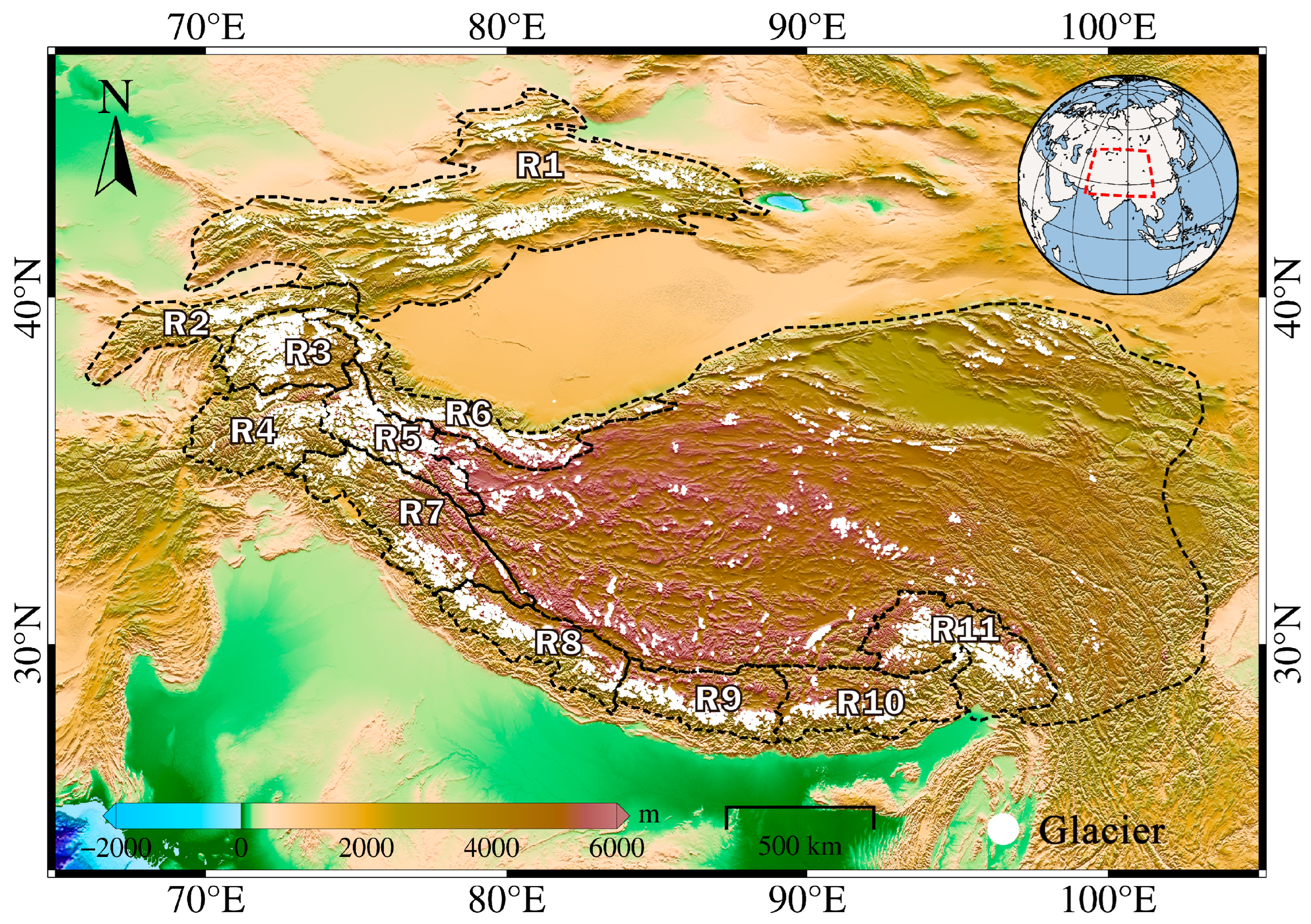
2. Studied Area
3. Data and Methods
3.1. Data
3.1.1. GRACE Mascon Products
3.1.2. Meteorological Data
3.1.3. ENSO
3.2. Methods
3.2.1. Empirical Orthogonal Function
3.2.2. Wavelet Amplitude–Period Spectrum Analysis
3.2.3. Singular Spectral Analysis
4. Results
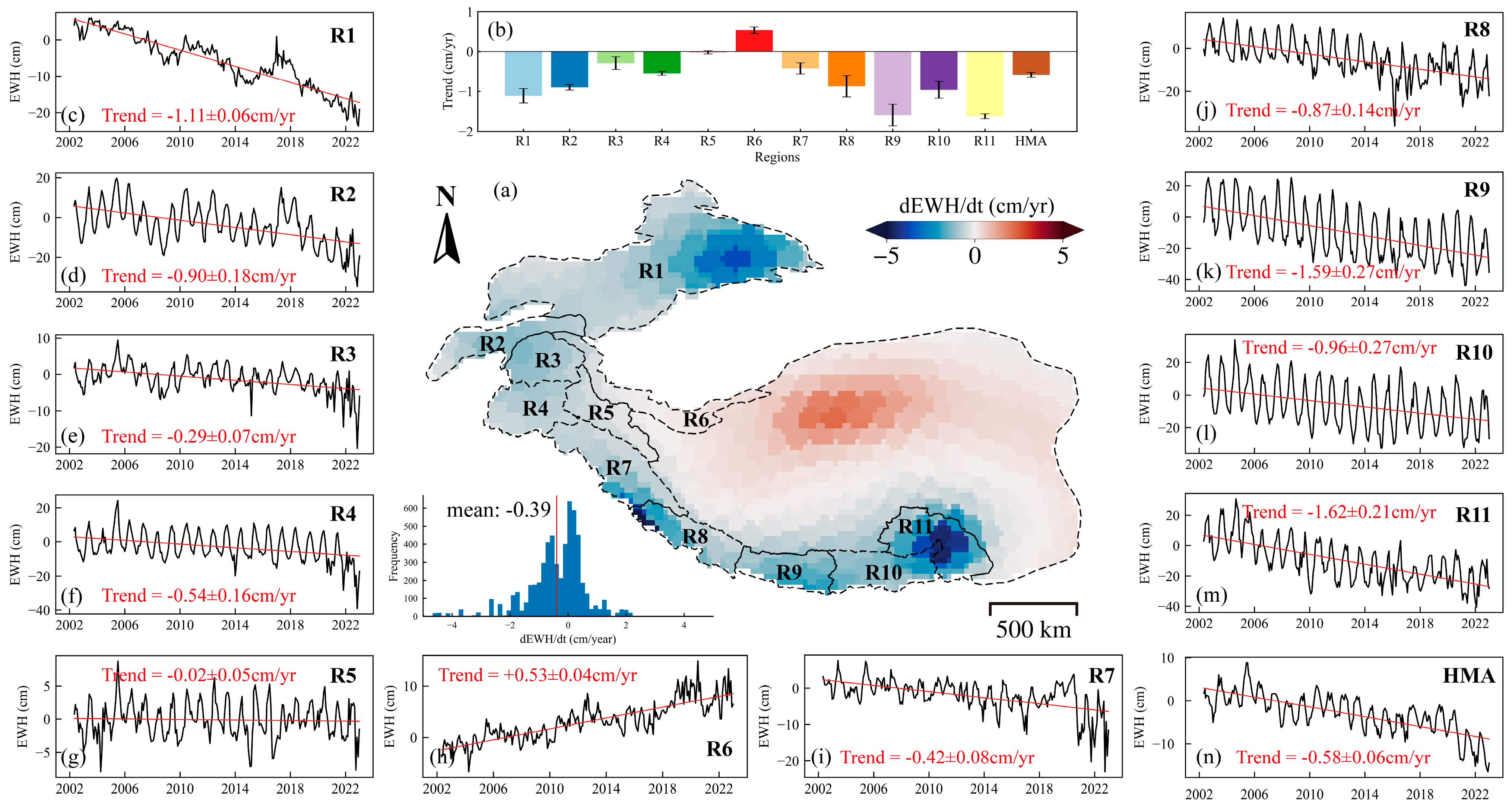
4.1. Spatial Trends and Time Series of Glacier Mass Changes in HMA
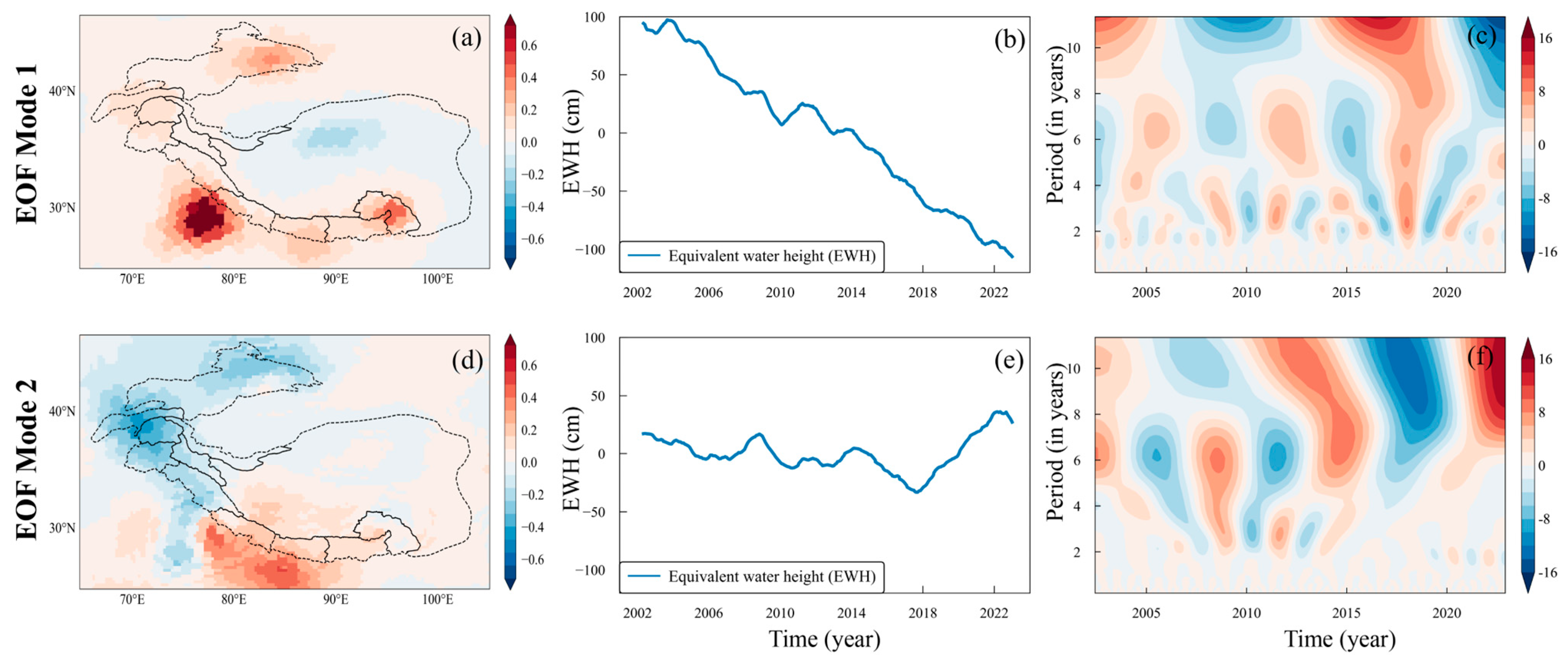
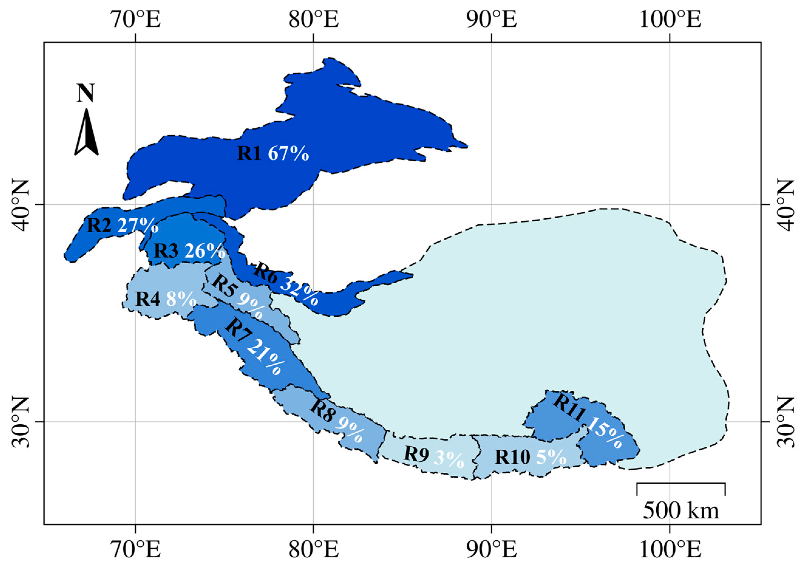
4.2. EOF of Glacial Change
4.3. SSA
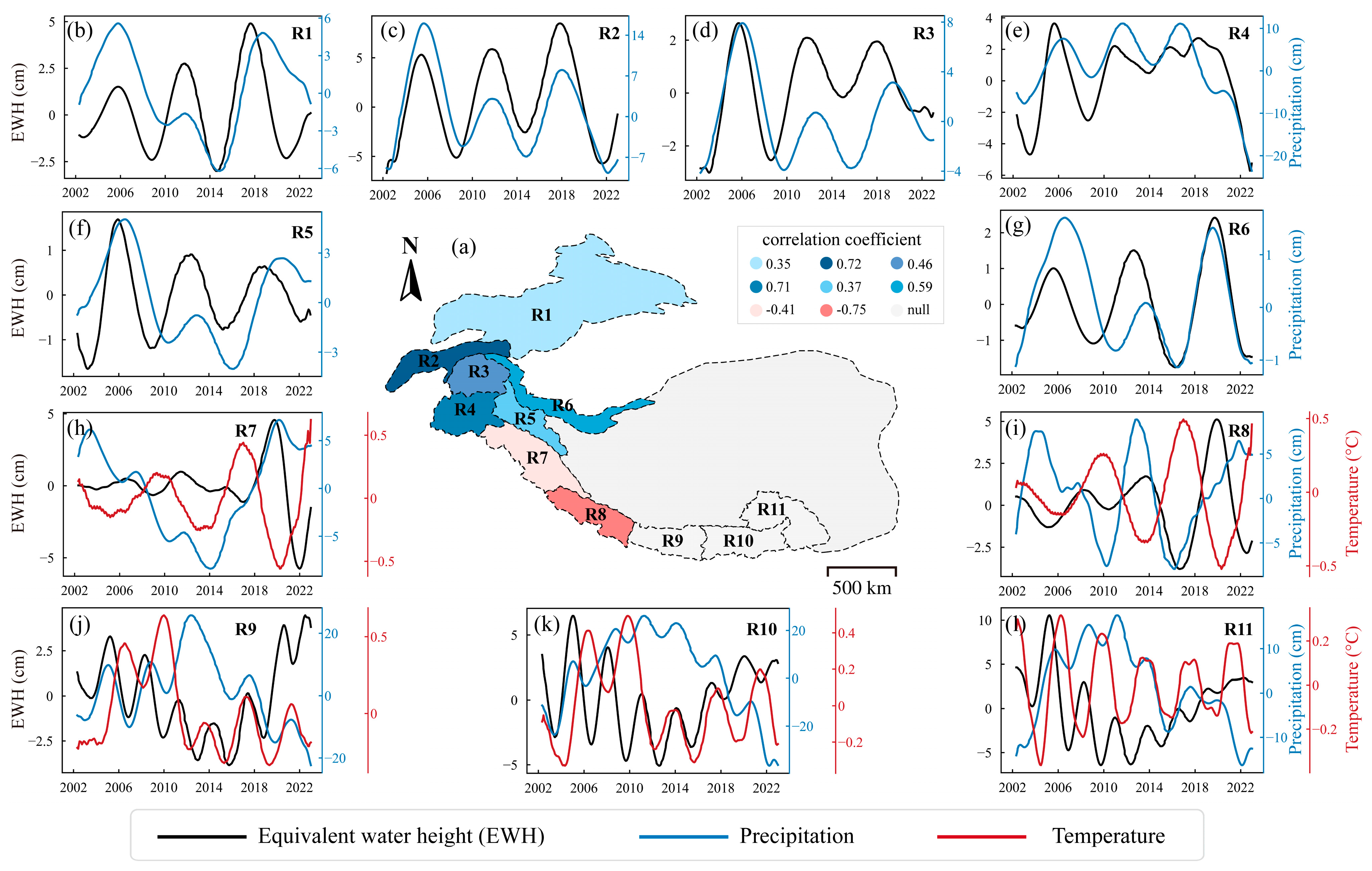
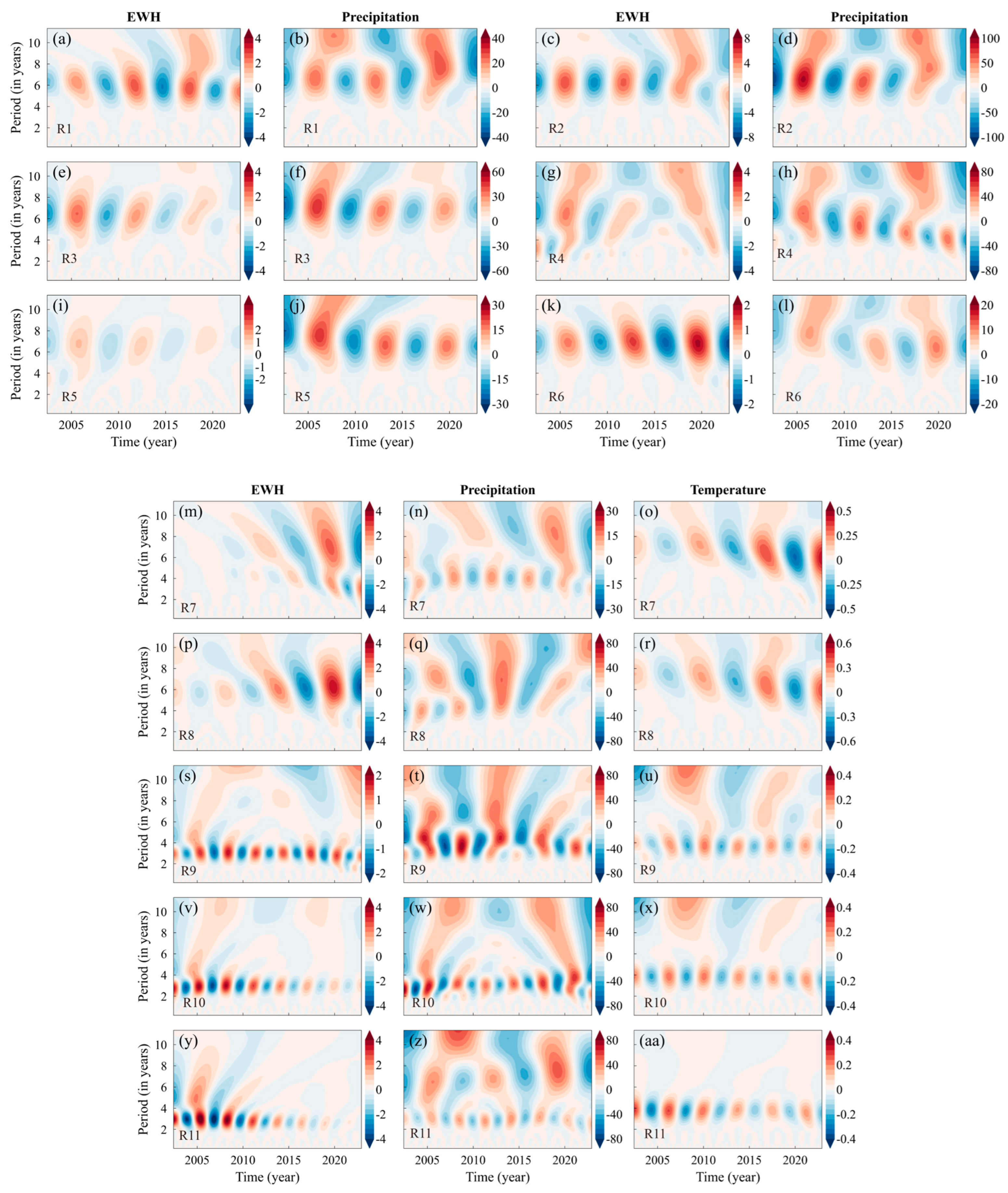
4.3.1. Correlation Analysis between Precipitation, Temperature and Mass on Interannual Scale
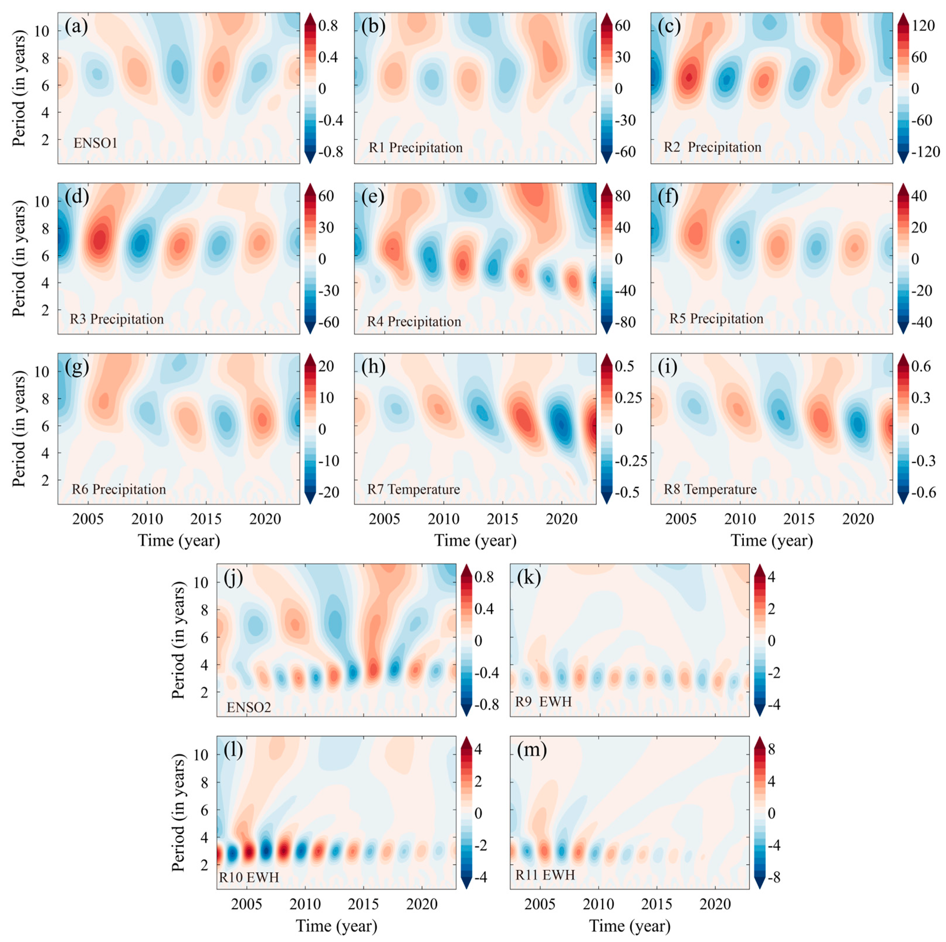
4.3.2. Correlation Analysis with ENSO
5. Discussion
5.1. HMA and Climate Indices
5.2. Spatial Heterogeneity in the HMA
6. Conclusions
Author Contributions
Funding
Data Availability Statement
Conflicts of Interest
References
- Immerzeel, W.W.; van Beek, L.P.H.; Bierkens, M.F.P. Climate Change Will Affect the Asian Water Towers. Science 2010, 328, 1382–1385. [Google Scholar] [CrossRef] [PubMed]
- Zemp, M.; Hoelzle, M.; Haeberli, W. Six decades of glacier mass-balance observations: A review of the worldwide monitoring network. Ann. Glaciol. 2009, 50, 101–111. [Google Scholar] [CrossRef]
- Haeberli, W.; Cihlar, J.; Barry, R.G. Glacier monitoring within the Global Climate Observing System. Ann. Glaciol. 2000, 31, 241–246. [Google Scholar] [CrossRef]
- Azam, M.F.; Ramanathan, A.; Wagnon, P.; Vincent, C.; Linda, A.; Berthier, E.; Sharma, P.; Mandal, A.; Angchuk, T.; Singh, V.B.; et al. Meteorological conditions, seasonal and annual mass balances of Chhota Shigri Glacier, western Himalaya, India. Ann. Glaciol. 2016, 57, 328–338. [Google Scholar] [CrossRef]
- Kumar, P.; Saharwardi, M.S.; Banerjee, A.; Azam, M.F.A.; Dubey, A.K.; Murtugudde, R. Snowfall Variability Dictates Glacier Mass Balance Variability in Himalaya-Karakoram. Sci. Rep. 2019, 9, 18192. [Google Scholar] [CrossRef]
- Luthcke, S.B.; Arendt, A.A.; Rowlands, D.D.; McCarthy, J.J.; Larsen, C.F. Recent glacier mass changes in the Gulf of Alaska region from GRACE mascon solutions. J. Glaciol. 2008, 54, 767–777. [Google Scholar] [CrossRef]
- Chen, J.L.; Wilson, C.R.; Tapley, B.D.; Blankenship, D.D.; Ivins, E.R. Patagonia icefield melting observed by gravity recovery and climate experiment (GRACE). Geophys. Res. Lett. 2007, 34, L22501. [Google Scholar] [CrossRef]
- Velicogna, I.; Mohajerani, Y.; Geruo, A.; Landerer, F.; Mouginot, J.; Noel, B.; Rignot, E.; Sutterley, T.; van den Broeke, M.; van Wessem, M.; et al. Continuity of Ice Sheet Mass Loss in Greenland and Antarctica From the GRACE and GRACE Follow-On Missions. Geophys. Res. Lett. 2020, 47, e2020GL087291. [Google Scholar] [CrossRef]
- Moiwo, J.P.; Yang, Y.H.; Tao, F.L.; Lu, W.X.; Han, S.M. Water storage change in the Himalayas from the Gravity Recovery and Climate Experiment (GRACE) and an empirical climate model. Water Resour. Res. 2011, 47, W07521. [Google Scholar] [CrossRef]
- Song, C.; Ke, L.; Huang, B.; Richards, K.S. Can mountain glacier melting explains the GRACE-observed mass loss in the southeast Tibetan Plateau: From a climate perspective? Glob. Planet. Chang. 2015, 124, 1–9. [Google Scholar] [CrossRef]
- Jiao, J.J.; Zhang, X.T.; Liu, Y.; Kuang, X.X. Increased Water Storage in the Qaidam Basin, the North Tibet Plateau from GRACE Gravity Data. PLoS ONE 2015, 10, e0141442. [Google Scholar] [CrossRef] [PubMed]
- Meng, F.; Su, F.; Li, Y.; Tong, K. Changes in Terrestrial Water Storage During 2003–2014 and Possible Causes in Tibetan Plateau. J. Geophys. Res.-Atmos. 2019, 124, 2909–2931. [Google Scholar] [CrossRef]
- Liu, X.; Xu, Z.; Yang, H.; Vaghefi, S.A. Responses of the Glacier Mass Balance to Climate Change in the Tibetan Plateau During 1975–2013. J. Geophys. Res.-Atmos. 2021, 126, e2019JD032132. [Google Scholar] [CrossRef]
- Wang, L.M.; Wang, J.X.; Wang, L.C.; Zhu, L.P.; Li, X.O. Terrestrial water storage regime and its change in the endorheic Tibetan Plateau. Sci. Total Environ. 2022, 815, 152729. [Google Scholar] [CrossRef] [PubMed]
- Gao, G.L.; Zhao, J.; Wang, J.X.; Zhao, G.Z.; Chen, J.Y.; Li, Z.P. Spatiotemporal Variation and Driving Analysis of Groundwater in the Tibetan Plateau Based on GRACE Downscaling Data. Water 2022, 14, 3302. [Google Scholar] [CrossRef]
- Xu, M.; Ye, B.S.; Zhao, Q.D.; Zhang, S.Q.; Wang, J. Estimation of water balance in the source region of the Yellow River based on GRACE satellite data. J. Arid Land 2013, 5, 384–395. [Google Scholar] [CrossRef]
- Li, X.Y.; Long, D.; Scanlon, B.R.; Mann, M.E.; Li, X.D.; Tian, F.Q.; Sun, Z.L.; Wang, G.Q. Climate change threatens terrestrial water storage over the Tibetan Plateau. Nat. Clim. Chang. 2022, 12, 801–807. [Google Scholar] [CrossRef]
- Becker, M.; Llovel, W.; Cazenave, A.; Guentner, A.; Cretaux, J.F. Recent hydrological behavior of the East African great lakes region inferred from GRACE, satellite altimetry and rainfall observations. C. R. Geosci. 2010, 342, 223–233. [Google Scholar] [CrossRef]
- Anyah, R.O.; Forootan, E.; Awange, J.; Khaki, M. Understanding linkages between global climate indices and terrestrial water storage changes over Africa using GRACE products. Sci. Total Environ. 2018, 635, 1405–1416. [Google Scholar] [CrossRef]
- Yao, C.L.; Luo, Z.C.; Wang, H.H.; Li, Q.; Zhou, H. GRACE-Derived Terrestrial Water Storage Changes in the Inter-Basin Region and Its Possible Influencing Factors: A Case Study of the Sichuan Basin, China. Remote Sens. 2016, 8, 444. [Google Scholar] [CrossRef]
- Miles, E.; McCarthy, M.; Dehecq, A.; Kneib, M.; Fugger, S.; Pellicciotti, F. Health and sustainability of glaciers in High Mountain Asia. Nat. Commun. 2021, 12, 2868. [Google Scholar] [CrossRef] [PubMed]
- Save, H.; Bettadpur, S.; Tapley, B.D. High-resolution CSR GRACE RL05 mascons. J. Geophys. Res.-Solid Earth 2016, 121, 7547–7569. [Google Scholar] [CrossRef]
- Sun, Y.; Riva, R.; Ditmar, P. Optimizing estimates of annual variations and trends in geocenter motion and J2 from a combination of GRACE data and geophysical models. J. Geophys. Res.-Solid Earth 2016, 121, 8352–8370. [Google Scholar] [CrossRef]
- Swenson, S.; Chambers, D.; Wahr, J. Estimating geocenter variations from a combination of GRACE and ocean model output. J. Geophys. Res.-Solid Earth 2008, 113, B08410. [Google Scholar] [CrossRef]
- Dobslaw, H.; Bergmann-Wolf, I.; Dill, R.; Poropat, L.; Thomas, M.; Dahle, C.; Esselborn, S.; König, R.; Flechtner, F. A new high-resolution model of non-tidal atmosphere and ocean mass variability for de-aliasing of satellite gravity observations: AOD1B RL06. Geophys. J. Int. 2017, 211, 263–269. [Google Scholar] [CrossRef]
- Zou, Y.; Kuang, X.; Feng, Y.; Jiao, J.J.; Liu, J.; Wang, C.; Fan, L.; Wang, Q.; Chen, J.; Ji, F.; et al. Solid Water Melt Dominates the Increase of Total Groundwater Storage in the Tibetan Plateau. Geophys. Res. Lett. 2022, 49, e2022GL100092. [Google Scholar] [CrossRef]
- Yi, S.; Sneeuw, N. Filling the Data Gaps Within GRACE Missions Using Singular Spectrum Analysis. J. Geophys. Res.-Solid Earth 2021, 126, e2020JB021227. [Google Scholar] [CrossRef]
- Harris, I.; Osborn, T.J.; Jones, P.; Lister, D. Version 4 of the CRU TS monthly high-resolution gridded multivariate climate dataset. Sci. Data 2020, 7, 109. [Google Scholar] [CrossRef]
- Wahr, J.; Molenaar, M.; Bryan, F. Time variability of the Earth’s gravity field: Hydrological and oceanic effects and their possible detection using GRACE. J. Geophys. Res.-Solid Earth 1998, 103, 30205–30229. [Google Scholar] [CrossRef]
- Pearson, K. On lines and planes of closest fit to systems of points in space. Philos. Mag. 1901, 2, 559–572. [Google Scholar] [CrossRef]
- Lorenz, E. Empirical Orthogonal Functions and Statistical Weather Prediction. Stat. Forecast. 1956, 1, 52. [Google Scholar]
- Hannachi, A.; Jolliffe, I.T.; Stephenson, D.B. Empirical orthogonal functions and related techniques in atmospheric science: A review. Int. J. Climatol. 2007, 27, 1119–1152. [Google Scholar] [CrossRef]
- Bhattacharya, A.; Bolch, T.; Mukherjee, K.; King, O.; Menounos, B.; Kapitsa, V.; Neckel, N.; Yang, W.; Yao, T.D. High Mountain Asian glacier response to climate revealed by multi-temporal satellite observations since the 1960s. Nat. Commun. 2021, 12, 4133. [Google Scholar] [CrossRef]
- Broomhead, D.S.; King, G.P. Extracting Qualitative Dynamics from Experimental-Data. Physica D 1986, 20, 217–236. [Google Scholar] [CrossRef]
- Wyatt, M.G.; Kravtsov, S.; Tsonis, A.A. Atlantic Multidecadal Oscillation and Northern Hemisphere’s climate variability. Clim. Dyn. 2012, 38, 929–949. [Google Scholar] [CrossRef]
- Kondrashov, D.; Berloff, P. Stochastic modeling of decadal variability in ocean gyres. Geophys. Res. Lett. 2015, 42, 1543–1553. [Google Scholar] [CrossRef]
- Chen, Q.; van Dam, T.; Sneeuw, N.; Collilieux, X.; Weigelt, M.; Rebischung, P. Singular spectrum analysis for modeling seasonal signals from GPS time series. J. Geodyn. 2013, 72, 25–35. [Google Scholar] [CrossRef]
- Jing, W.; Zhang, P.; Zhao, X. A comparison of different GRACE solutions in terrestrial water storage trend estimation over Tibetan Plateau. Sci. Rep. 2019, 9, 1765. [Google Scholar] [CrossRef]
- Zhan, J.G.; Shi, H.L.; Wang, Y.; Yao, Y.X. Complex principal component analysis of mass balance changes on the Qinghai-Tibetan Plateau. Cryosphere 2017, 11, 1487–1499. [Google Scholar] [CrossRef]
- Yang, W.; Guo, X.F.; Yao, T.D.; Zhu, M.L.; Wang, Y.J. Recent accelerating mass loss of southeast Tibetan glaciers and the relationship with changes in macroscale atmospheric circulations. Clim. Dyn. 2016, 47, 805–815. [Google Scholar] [CrossRef]
- Wang, Z.B.; Wu, R.G.; Yang, S.; Lu, M.M. An Interdecadal Change in the Influence of ENSO on the Spring Tibetan Plateau Snow-Cover Variability in the Early 2000s. J. Clim. 2022, 35, 725–743. [Google Scholar] [CrossRef]
- Wang, Q.Y.; Yi, S.; Sun, W.K. Precipitation-driven glacier changes in the Pamir and Hindu Kush mountains. Geophys. Res. Lett. 2017, 44, 2817–2824. [Google Scholar] [CrossRef]
- Mandal, A.; Ramanathan, A.L.; Angchuk, T.; Soheb, M.; Singh, V.B. Unsteady state of glaciers (Chhota Shigri and Hamtah) and climate in Lahaul and Spiti region, western Himalayas: A review of recent mass loss. Environ. Earth Sci. 2016, 75, 1233. [Google Scholar] [CrossRef]
- Hu, S.; Wu, B.; Zhou, T.J.; Yu, Y.Q. Dominant Anomalous Circulation Patterns of Tibetan Plateau Summer Climate Generated by ENSO-Forced and ENSO-Independent Teleconnections. J. Clim. 2022, 35, 1679–1694. [Google Scholar] [CrossRef]
- Wang, C.X.; Ma, Z.F. Quasi-3-yr Cycle of Rainy Season Precipitation in Tibet Related to Different Types of ENSO during 1981-2015. J. Meteorol. Res. 2018, 32, 181–190. [Google Scholar] [CrossRef]
- Yang, X.X.; Yao, T.D.; Deji; Zhao, H.B.; Xu, B.Q. Possible ENSO Influences on the Northwestern Tibetan Plateau Revealed by Annually Resolved Ice Core Records. J. Geophys. Res.-Atmos. 2018, 123, 3857–3870. [Google Scholar] [CrossRef]
- Wu, J.; Wu, Z. Inter-decadal change of the spring North Atlantic Oscillation impact on the summer Pamir–Tienshan snow cover. Int. J. Climatol. 2019, 39, 629–642. [Google Scholar] [CrossRef]
- Kang, S.; Qin, D.; Ren, J.; Zhang, Y.; Kaspari, S.; Mayewski, P.A.; Hou, S. Annual accumulation in the Mt. nyainqentanglha ice core, southern Tibetan plateau, China: Relationships to atmospheric circulation over Asia. Arct. Antarct. Alp. Res. 2007, 39, 663–670. [Google Scholar] [CrossRef]
- Xu, H.; Hong, Y.T.; Hong, B.; Zhu, Y.X.; Wang, Y. Influence of ENSO on multi-annual temperature variations at Hongyuan, NE Qinghai-Tibet plateau: Evidence from δ13 C of spruce tree rings. Int. J. Climatol. 2010, 30, 120–126. [Google Scholar] [CrossRef]
- Wang, S.S.; Huang, J.P.; He, Y.L.; Guan, Y.P. Combined effects of the Pacific Decadal Oscillation and El Nino-Southern Oscillation on Global Land Dry-Wet Changes. Sci. Rep. 2014, 4, 6651. [Google Scholar] [CrossRef]
- Thirumalai, K.; DiNezio, P.N.; Okumura, Y.; Deser, C. Extreme temperatures in Southeast Asia caused by El Nino and worsened by global warming. Nat. Commun. 2017, 8, 15531. [Google Scholar] [CrossRef] [PubMed]
- Zhu, Y.; Liu, S.; Yi, Y.; Li, W.; Zhang, S. Spatiotemporal Changes of Terrestrial Water Storage in Three Parallel River Basins and Its Response to ENSO. Mt. Res. 2020, 38, 165–179. [Google Scholar] [CrossRef]
- Xu, H.; Hou, S.G.; Pang, H.X.; Wang, C.M. Effects of ENSO on the major ion record of a Qomolangma (Mount Everest) ice core. Ann. Glaciol. 2016, 57, 282–288. [Google Scholar] [CrossRef]
- Li, J.P.; Feng, J.; Li, Y. A possible cause of decreasing summer rainfall in northeast Australia. Int. J. Climatol. 2012, 32, 995–1005. [Google Scholar] [CrossRef]
- Zhang, Q.B.; Evans, M.N.; Lyu, L. Moisture dipole over the Tibetan Plateau during the past five and a half centuries. Nat. Commun. 2015, 6, 8062. [Google Scholar] [CrossRef]
- Wu, G.; Zhang, Y. Tibetan Plateau Forcing and the Timing of the Monsoon Onset over South Asia and the South China Sea. Mon. Weather Rev. 1998, 126, 913–927. [Google Scholar] [CrossRef]
- Zhao, Z.Z.; Cao, J.J.; Shen, Z.X.; Xu, B.Q.; Zhu, C.S.; Chen, L.W.A.; Su, X.L.; Liu, S.X.; Han, Y.M.; Wang, G.H. Aerosol particles at a high-altitude site on the Southeast Tibetan Plateau, China: Implications for pollution transport from South Asia. J. Geophys. Res.-Atmos. 2013, 118, 11360–11375. [Google Scholar] [CrossRef]
- Li, G.P.; Yu, Z.B.; Wang, W.G.; Ju, Q.; Chen, X. Analysis of the spatial Distribution of precipitation and topography with GPM data in the Tibetan Plateau. Atmos. Res. 2021, 247, 105259. [Google Scholar] [CrossRef]
- Hu, S.; Zhou, T.J.; Wu, B. Impact of Developing ENSO on Tibetan Plateau Summer Rainfall. J. Clim. 2021, 34, 3385–3400. [Google Scholar] [CrossRef]
- He, S.P.; Wang, H.J. Oscillating Relationship between the East Asian Winter Monsoon and ENSO. J. Clim. 2013, 26, 9819–9838. [Google Scholar] [CrossRef]
- Yao, T.; Bolch, T.; Chen, D.; Gao, J.; Immerzeel, W.; Piao, S.; Su, F.; Thompson, L.; Wada, Y.; Wang, L.; et al. The imbalance of the Asian water tower. Nat. Rev. Earth Environ. 2022, 3, 618–632. [Google Scholar] [CrossRef]
- Anjum, M.N.; Ding, Y.J.; Shangguan, D.H. Simulation of the projected climate change impacts on the river flow regimes under CMIP5 RCP scenarios in the westerlies dominated belt, northern Pakistan. Atmos. Res. 2019, 227, 233–248. [Google Scholar] [CrossRef]
- Yi, S.; Sun, W. Evaluation of glacier changes in high-mountain Asia based on 10 year GRACE RL05 models. J. Geophys. Res. Solid Earth 2014, 119, 2504–2517. [Google Scholar] [CrossRef]
- Rekier, J.; Chao, B.F.; Chen, J.L.; Dehant, V.; Rosat, S.; Zhu, P. Earth’s Rotation: Observations and Relation to Deep Interior. Surv. Geophys. 2022, 43, 149–175. [Google Scholar] [CrossRef]
- Cazenave, A.; Pfeffer, J.; Mandea, M.; Dehant, V. ESD Ideas: A 6-year oscillation in the whole Earth system? Earth Syst. Dynam. 2023, 14, 733–735. [Google Scholar] [CrossRef]
- Pan, Y.J.; Jiang, W.P.; Ding, H.; Shum, C.K.; Jiao, J.S.; Xiao, Y.X.; Wu, Q.W. Interannual variability of vertical land motion over High Mountain Central Asia from GPS and GRACE/GRACE-FO observations. GPS Solut. 2023, 27, 168. [Google Scholar] [CrossRef]
- Chen, J.L.; Wilson, C.R.; Kuang, W.J.; Chao, B.F. Interannual Oscillations in Earth Rotation. J. Geophys. Res.-Solid Earth 2019, 124, 13404–13414. [Google Scholar] [CrossRef]
- Pfeffer, J.; Cazenave, A.; Rosat, S.; Moreira, L.; Mandea, M.; Dehant, V.; Coupry, B. A 6-year cycle in the Earth system. Glob. Planet. Chang. 2023, 229, 104245. [Google Scholar] [CrossRef]
- Chao, B.F.; Yu, Y. Variation of the equatorial moments of inertia associated with a 6-year westward rotary motion in the Earth. Earth Planet. Sci. Lett. 2020, 542, 116316. [Google Scholar] [CrossRef]
- Deng, C.; Zhang, W. Spatial distribution pattern of degree–day factors of glaciers on the Qinghai–Tibetan Plateau. Environ. Monit. Assess. 2018, 190, 475. [Google Scholar] [CrossRef]
- Zhu, M.; Yao, T.; Xie, Y.; Xu, B.; Yang, W.; Yang, S. Mass balance of Muji Glacier, northeastern Pamir, and its controlling climate factors. J. Hydrol. 2020, 590, 125447. [Google Scholar] [CrossRef]
- Shi, Y.F.; Liu, S.Y. Estimation on the response of glaciers in China to the global warming in the 21st century. Chin. Sci. Bull. 2000, 45, 668–672. [Google Scholar] [CrossRef]
- Zhang, Y.; Hirabayashi, Y.; Liu, S.Y. Catchment-scale reconstruction of glacier mass balance using observations and global climate data: Case study of the Hailuogou catchment, south-eastern Tibetan Plateau. J. Hydrol. 2012, 444, 146–160. [Google Scholar] [CrossRef]
- Duan, A.; Wu, G.; Zhang, Q.; Liu, Y. New proofs of the recent climate warming over the Tibetan Plateau as a result of the increasing greenhouse gases emissions. Chin. Sci. Bull. 2006, 51, 1396–1400. [Google Scholar] [CrossRef]
- Duan, A.; Wu, G. Change of cloud amount and the climate warming on the Tibetan Plateau. Geophys. Res. Lett. 2006, 33, L22704. [Google Scholar] [CrossRef]
- Gao, K.; Duan, A.; Chen, D.; Wu, G. Surface energy budget diagnosis reveals possible mechanism for the different warming rate among Earth’s three poles in recent decades. Sci. Bull. 2019, 64, 1140–1143. [Google Scholar] [CrossRef] [PubMed]
- Lüthi, Z.L.; Škerlak, B.; Kim, S.W.; Lauer, A.; Mues, A.; Rupakheti, M.; Kang, S. Atmospheric brown clouds reach the Tibetan Plateau by crossing the Himalayas. Atmos. Chem. Phys. 2015, 15, 6007–6021. [Google Scholar] [CrossRef]
- Cui, X.; Graf, H.-F. Recent land cover changes on the Tibetan Plateau: A review. Clim. Chang. 2009, 94, 47–61. [Google Scholar] [CrossRef]
- Wen, Z.; Yi, S.; Sun, W. Significant contribution of the Tianshan lakes to their water storage and water resources. J. Hydrol. Reg. Stud. 2024, 53, 101813. [Google Scholar] [CrossRef]

Disclaimer/Publisher’s Note: The statements, opinions and data contained in all publications are solely those of the individual author(s) and contributor(s) and not of MDPI and/or the editor(s). MDPI and/or the editor(s) disclaim responsibility for any injury to people or property resulting from any ideas, methods, instructions or products referred to in the content. |
© 2024 by the authors. Licensee MDPI, Basel, Switzerland. This article is an open access article distributed under the terms and conditions of the Creative Commons Attribution (CC BY) license (https://creativecommons.org/licenses/by/4.0/).
Share and Cite
Wang, Y.; Zhan, J.; Shi, H.; Chen, J. Interannual Glacial Mass Changes in High Mountain Asia and Connections to Climate Variability. Remote Sens. 2024, 16, 3426. https://doi.org/10.3390/rs16183426
Wang Y, Zhan J, Shi H, Chen J. Interannual Glacial Mass Changes in High Mountain Asia and Connections to Climate Variability. Remote Sensing. 2024; 16(18):3426. https://doi.org/10.3390/rs16183426
Chicago/Turabian StyleWang, Yifan, Jingang Zhan, Hongling Shi, and Jianli Chen. 2024. "Interannual Glacial Mass Changes in High Mountain Asia and Connections to Climate Variability" Remote Sensing 16, no. 18: 3426. https://doi.org/10.3390/rs16183426
APA StyleWang, Y., Zhan, J., Shi, H., & Chen, J. (2024). Interannual Glacial Mass Changes in High Mountain Asia and Connections to Climate Variability. Remote Sensing, 16(18), 3426. https://doi.org/10.3390/rs16183426