County-Level Cultivated Land Quality Evaluation Using Multi-Temporal Remote Sensing and Machine Learning Models: From the Perspective of National Standard

Abstract

Scientific evaluation of cultivated land quality (CLQ) is necessary for promoting rational utilization of cultivated land and achieving one of the Sustainable Development Goals (SDGs): Zero Hunger. However, the CLQ evaluation system proposed in previous studies was diversified, and the methods were inefficient. In this study, based on China’s first national standard “Cultivated Land Quality Grade” (GB/T 33469-2016), we constructed a unified county-level CLQ evaluation system by selecting 15 indicators from five aspects—site condition, environmental condition, physicochemical property, nutrient status and field management—and used the Delphi method to calculate the membership degree of the indicators. Taking Jimo district of Shandong Province, China, as a case study, we compared the performance of three machine learning models, including random forest, AdaBoost, and support vector regression, to evaluate CLQ using multi-temporal remote sensing data. The comprehensive index method was used to reveal the spatial distribution of CLQ. The results showed that the CLQ evaluation based on multi-temporal remote sensing data and machine learning model was efficient and reliable, and the evaluation results had a significant positive correlation with crop yield (r was 0.44, p < 0.001). The proportions of cultivated land of high-, medium- and poor-quality were 27.43%, 59.37% and 13.20%, respectively. The CLQ in the western part of the study area was better, while it was worse in the eastern and central parts. The main limiting factors include irrigation capacity and texture configuration. Accordingly, a series of targeted measures and policies were suggested, such as strengthening the construction of farmland water conservancy facilities, deep tillage of soil and continuing to construct well-facilitated farmland. This study proposed a fast and reliable method for evaluating CLQ, and the results are helpful to promote the protection of cultivated land and ensure food security.

1. Introduction

Cultivated land is the cornerstone of human survival and social development [1,2]. Cultivated land quality (CLQ) is closely related to food security on a global or regional scale [3,4,5]. However, some factors, such as urban expansion, climate change and conflict, are seriously threatening the CLQ in many regions of the world [6,7]. As the largest developing country in the world, China’s cultivated land of medium- and low-grade accounts for about 70%, indicating that it was generally poor [8,9,10,11]. Therefore, to ensure food security and maintain social stability, the Chinese government implemented a series of strict cultivated land protection policies [12,13,14]. For example, China put forward the concept of “trinity” protection of cultivated land, emphasizing that the quantity is the premise, the quality is the key and the ecological environment is the fundament [2,15]. Considering the decreasing quantity of cultivated land, improving the quality and ecological environment of cultivated land is an effective measure to improve grain yield and quality [9,16]. Scientific evaluation of CLQ can help stakeholders understand its current situation and provide targeted improvement measures [17,18]. Therefore, it is valuable to carry out research on CLQ evaluation.

Constructing a reasonable evaluation system is the key of CLQ evaluation [16,19]. However, due to the different evaluation purposes, there is no consensus on the intension of CLQ in the world, which leads to the diversification of the evaluation system [12,20]. Previous studies analyzed the intension of CLQ from the perspectives of soil fertility [21], soil quality [22], soil health [23], cultivated land productivity [24] and cultivated land sustainability [25]. The comprehensive evaluation of CLQ based on multiple factors has attracted more and more attention. For example, CLQ was defined as production capacity quality and environmental quality [10]. A previous study selected 28 indicators from three aspects: basic condition, health condition and ecological condition [2]. In terms of cultivated land ecosystem, the CLQ evaluation system was constructed from five aspects: background, efficiency, sustainability, environment and landscape quality [4]. The CLQ evaluation system established by existing studies was built for specific areas and evaluation purposes, which was not universal and the evaluation techniques were not uniform.

To unify the procedures and methods of CLQ evaluation, the Chinese government implemented a series of national standards and norms. For example, the Ministry of Natural Resources formulated the “Regulation for Gradation on Agriculture Land Quality” (RGALQ) (GB/T 28407-2012) [26], which was used to comprehensively evaluate the CLQ by revising the natural quality, utilization level and economic level of cultivated land step by step [8,26]. To protect the soil environment of cultivated land, the Ministry of Ecological Environment formulated the “Soil Environmental Quality—Risk Control Standard for Soil Contamination of Agricultural Land” (SEQ) (GB/T 15618-2018) [27]. The Ministry of Agriculture and Rural Affairs issued the “Rules for Soil Quality Survey and Assessment” (NY/T1634-2008) [28], which stipulated the methods, procedures and contents of the evaluation of cultivated land fertility and cultivated land environmental quality [28]. The “Methods for Investigation, Monitoring and Evaluation of Cultivated Land Quality”, for the first time, clarified the definition of CLQ, which refers to the ability of cultivated land fertility, soil health and field infrastructure to meet the sustainable production and quality safety of agricultural products [29]. Based on this, China’s first national standard “Cultivated Land Quality Grade” (CLQG) (GB/T33469-2016) was released, which specified the regional division of CLQ, the determination of indicators and the process of CLQ grade division. The CLQG divides the cultivated land of the country into nine regions, and the evaluation indicators of each region contain thirteen basic indicators and six regional supplementary indicators and clarify the meaning and acquisition methods of relevant evaluation indicators [30]. Compared with RGALQ and SEQ, the CLQG pays more attention to the comprehensive quality of cultivated land, including cultivated land fertility, soil health and field infrastructure. In addition, the evaluation indicators are targeted, the evaluation procedure is universal and the evaluation results are quantitative [31].

How to evaluate the CLQ efficiently and reliably is a global research hotspot [10,11,32]. The traditional CLQ evaluation method relied on a lot of field investigation, which was time-consuming and labor-intensive [19,33]. To obtain CLQ information at a regional scale quickly and shorten the evaluation period, remote sensing data have been widely adopted [24,32]. For example, multi-source remote sensing was used to evaluate CLQ in the northeast and south of China [11,19]. A CLQ inversion model was constructed based on high-resolution remote sensing data [34]. Considering this, the fusion of multi-source data, such as remote sensing, meteorology, topography and soil attributes, can more comprehensively characterize CLQ [25]. However, traditional statistical methods cannot reveal the nonlinear relationship between multi-source data [2]. Studies show that machine learning models can dig deep into the nonlinear or more complex relationship between multi-source data and CLQ [35,36]. For example, random forest (RF), AdaBoost, XGBoost, support vector regression (SVR) and decision tree (DT) have been widely used in CLQ evaluation [25,35,37]. However, due to the spatial variability of cultivated land type, topography, soil properties and field management, no one machine learning model is universally applicable [38,39]. Therefore, comparative studies are often needed for specific research areas and evaluation objectives.

The objective of CLQ evaluation should pay more attention to identify the main obstacle factors and put forward targeted improvement measures [2,20]. Many studies directly incorporated some obstacle factors, such as soil salinization [40], desertification [41] and erosion [42], into the CLQ evaluation system, but they ignored the obstacle degree of other indicators to CLQ. For example, when the soil nutrient content is low, the soil pH is too acidic or too alkaline or irrigation cannot be satisfied, they may become obstacle factors. Some studies have shown that irrigation capacity was mainly affected by farmland infrastructure, irrigation water reserves and other factors [43,44]. Therefore, to improve CLQ in a targeted manner, it is necessary to quantitatively evaluate the obstacle degree of each indicator to CLQ and analyze the causes of the obstacle. The minimum limiting factor method and obstacle factor diagnostic model are popular methods to identify obstacle factors. The former overemphasizes the contribution of the factor with the greatest degree of obstacle [10]. In fact, CLQ is often affected by multiple obstacle factors [2,19]. Based on the system theory, the obstacle factor diagnosis model can identify and analyze obstacle factors and rank the obstacle degree of the factors [17], so it is more suitable for CLQ evaluation.

The county-level administrative district is the basic unit for the management and protection of cultivated land in China [15,45]. China’s relevant national standards of CLQ evaluation take county-level administrative district as the evaluation unit, and the cultivated land can be managed and optimized directly according to the evaluation results. Therefore, it is urgent and meaningful to build a general CLQ evaluation system applicable to county and improve the efficiency and reliability of CLQ evaluation [19,45]. In view of the authority, comprehensiveness, science, standardization and operability of the “Cultivated Land Quality Grade” (GB/T 33469-2016) [30], this study constructed a unified CLQ evaluation indicator system based on this. Taking the Jimo district of Shandong Province, China, as a case study, we used multi-temporal remote sensing data and machine learning models to evaluate CLQ of the study area and revealed the spatial pattern of CLQ by comprehensive index method. Finally, the main limiting factors were identified by the obstacle factor diagnosis model. The main contributions of this study were as follows: (1) to provide an efficient and reproducible CLQ evaluation method applicable to county districts based on national standard with multi-temporal remote sensing and machine learning models; (2) to reveal the spatial pattern of CLQ in Jimo district and help stakeholders grasp the current situation of CLQ; and (3) to identify the main obstacle factors and provide targeted measures or policy recommendations.

2. Materials and Methods

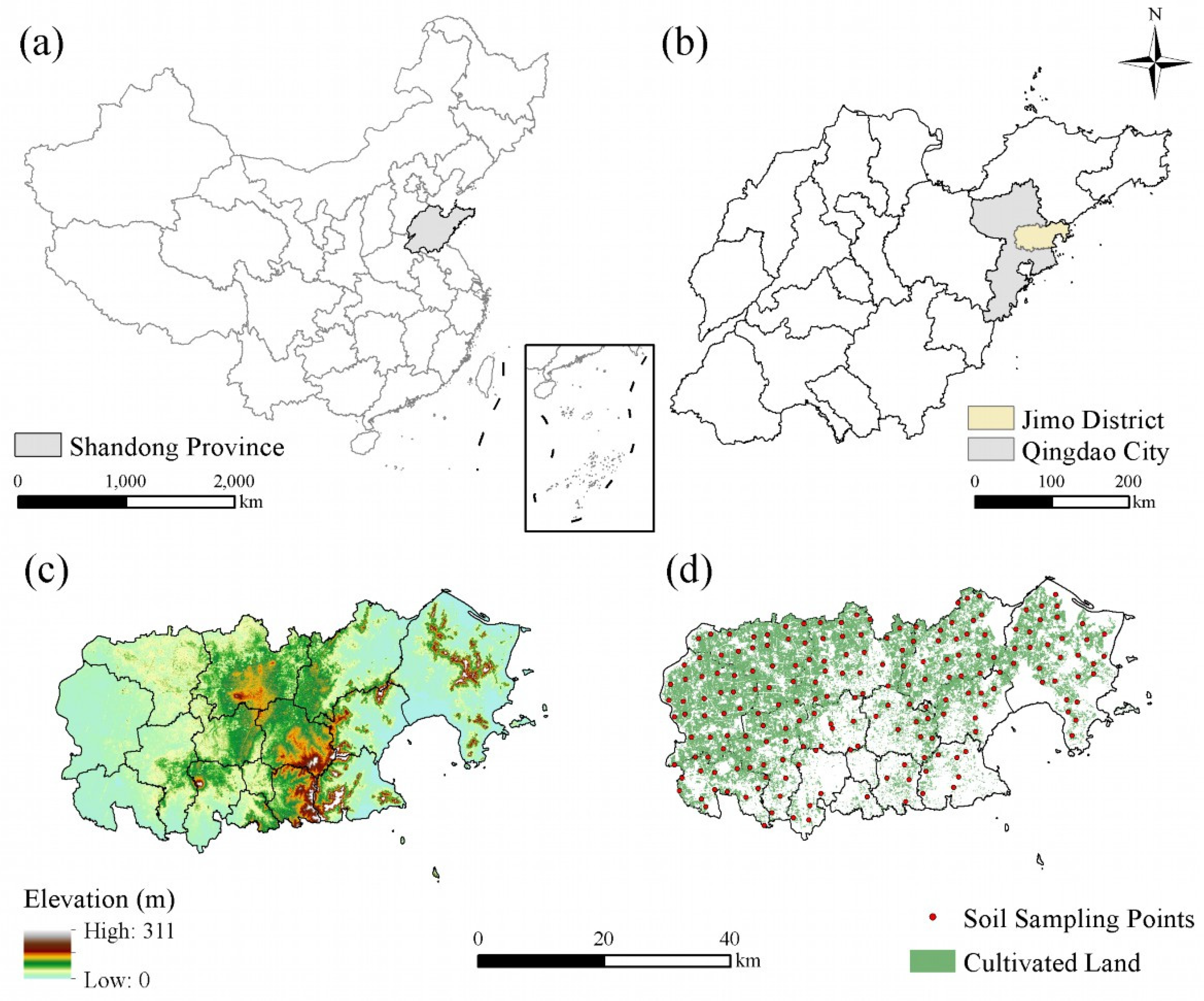
2.1. Study Area

We selected Jimo district of Shandong Province, China (120°07′–121°23′E, 36°18′–36°37′N), as a case study area (Figure 1). The study area consists of 11 streets and 4 towns with a total area of 1780 km². The landform is characterized by low mountains and hills, and the terrain is high in the middle and low in the east and west. The main soil types are brown loam, Shajiang black soil and tidal soil. The climate is a warm temperate monsoon continental climate area, with an average annual temperature of 12.1 °C, an average annual precipitation of 708.9 mm and an annual accumulated temperature of 4410 °C. Jimo district is a traditional agricultural area with cultivated land area of about 78,300 hectares and mainly dry land. The cultivation system in the study area is mainly two croppings a year, mainly wheat and maize rotation, accounting for nearly 90%.

2.2. Data Resources and Processing

2.2.1. Soil Sampling Data

A total of 195 soil surface samples (0–20 cm) were collected in the cultivated land area of the study area in October 2022 (Figure 1). We recorded the geographic location of all the soil sampling sites with a global positioning system. The soil indicators collected included soil organic matter (SOM), soil pH, available phosphorus (AP), available potassium (AK), soil bulk density (SBD), topographic position, effective soil layer thickness, texture configuration, thickness of ploughing layer, topsoil texture, irrigation capacity, drainage capacity, farmland forest network degree, biodiversity and cleanliness degree. The descriptive statistics of the soil sampling data are shown in

Table 1. Descriptive statistics of soil sampling data.

	Soil Organic Matter (g/kg)	Soil pH	Available Phosphorus (mg/kg)	Available Potassium (mg/kg)	Soil Bulk Density (g/cm3)
n	195	195	195	195	195
mean	14.98	5.89	38.43	105.28	1.48
min	4.09	2.86	3.60	19.00	1.11
max	30.70	8.32	225.20	280.00	1.81
std. dev	4.52	0.86	27.18	52.92	0.13
variance	20.43	0.73	738.70	2800.93	0.016
cv (%)	30.17	14.60	70.73	50.27	8.78

.

2.2.2. Satellite Data

Sentinel-2 images without cloud cover were obtained from European Space Agency (https://www.usgs.gov/) (accessed on 1 May 2023) on 18, 23 and 28 October 2022 to match the operational dates of soil sampling. We used SNAP software (version 6.0) to resample Sentinel-2 data with a unified spatial resolution of 10 m, extracted the band reflectance of blue band (B2), green band (B3), red band (B4), red edge 1 band (B5), red edge 2 band (B6), red edge 3 band (B7), near-infrared band (B8) and red edge 4 band (B8a) and calculated normalized difference vegetation index (NDVI), enhanced vegetation index (EVI) and soil-adjusted vegetation index (SAVI). The average values of band reflectance and vegetation index in the three periods were used as environmental variables to construct the prediction model of CLQ evaluation indicators.

2.2.3. Other Auxiliary Data

Meteorological data, including mean annual precipitation (MAP), mean annual temperature (MAT), accumulated temperature greater than 10 degrees Celsius, relative humidity and evaporation, were obtained from the National Meteorological Science Data Center (http:/data.cma.cn/) (accessed on 10 May 2023). The digital elevation model (DEM) was derived from the geospatial data cloud (http://www.gscloud.cn/) (accessed on 28 May 2023). We used ArcGIS to extract elevation information and calculate slope, plane curvature, profile curvature and topographic wetness index. Meteorological and topographic data were used to predict CLQ evaluation indicators.

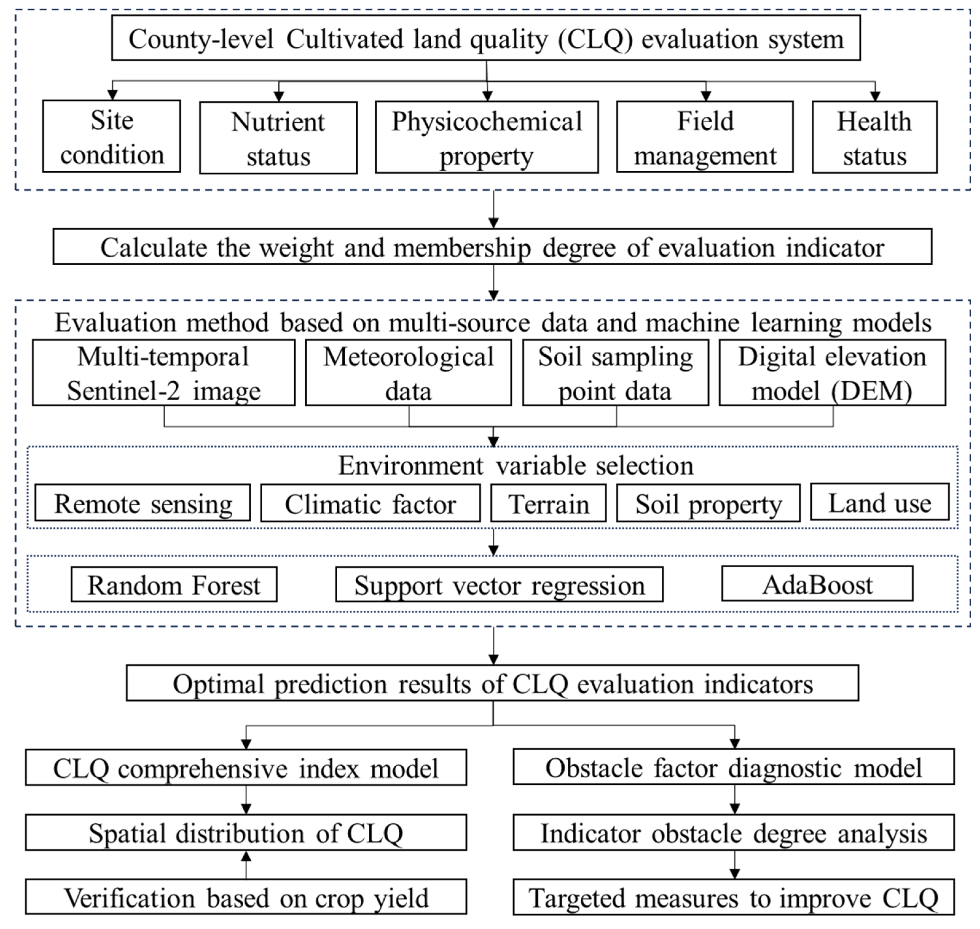
2.3. Methodological Framework for CLQ Evaluation

The evaluation process of CLQ includes five steps in this study (Figure 2). The first step is to construct the CLQ evaluation system according to the “Cultivated Land Quality Grade” (GB/T33469-2016) [30]. The second step is to use the analytic hierarchy process (AHP) [18] and the Delphi method [23] to calculate the weight and membership of the indicators. The third step is to construct the prediction model of CLQ evaluation indicator, including the selection of environmental variables, the training and verification of machine learning models. The purpose of model training is to enable machine learning models to automatically extract useful features through large amounts of training data and learn how to make predictions on new input data sets [37,46]. The purpose of model verification is to prevent machine learning models from overfitting and underfitting and to optimize the model [47,48]. The fourth step is the comprehensive evaluation of CLQ and verification of results. The fifth step is to identify the main obstacle factors by using the obstacle factor diagnosis model, aiming at providing targeted measures.

2.3.1. Construction of CLQ Evaluation System

CLQ Evaluation Indicators and Weight Coefficients

Based on the “Cultivated Land Quality Grade” (GB/T 33469-2016) [30], according to the principle of combining basic indicators and regional supplementary indicators, 15 evaluation indicators were selected from 5 aspects of site condition, environmental condition, physicochemical property, nutrient status and field management to construct the comprehensive evaluation system of CLQ, including 13 basic indicators, such as topographic position, effective soil layer thickness, texture configuration, topsoil texture, SBD, SOM, AP, AK, irrigation capacity, drainage capacity, farmland forest network degree, biodiversity and cleanliness degree, and 2 regional indicators, including thickness of ploughing layer and soil pH.

Topographic location, effective soil layer thickness, texture configuration and thickness of ploughing layer are the key criteria to measure the cultivability of cultivated land, and they are the most commonly used indicators to characterize the site conditions of cultivated land [12,18]. Soil pH, topsoil texture and SBD are key components of soil physicochemical properties [21]. Soil pH is closely related to the availability of soil nutrients [36]. Topsoil texture can affect the water and fertilizer retention ability of soil [25]. SBD has influence on soil permeability and soil temperature [8]. Nutrient status can represent soil fertility [49]. SOM, AP and AK are the most representative indicators of soil nutrients [50]. Farmland management is an important measure to improve CLQ [22]. For example, proper irrigation and drainage can ensure the healthy growth of crops [25]. Farmland forest network degree can improve the cultivated land environment and reduce soil erosion [16]. Biodiversity and cleaning degree were selected to characterize the health status of cultivated land, which is the core of ensuring the quality and safety of agricultural products [2]. Biodiversity can reflect the richness of cultivated soil vitality [51,52]. Cleaning degree can reflect the extent to which cultivated soil is affected by toxic and harmful substances such as heavy metals, pesticides and agricultural film residues [2,18].

It is very important to set the appropriate weight coefficient for each evaluation indicator. In this study, we consulted seven experts in the field of CLQ evaluation from the Chinese Academy of Agricultural Sciences, Shandong Agricultural University and Qingdao Agricultural University in the form of questionnaires. They ranked the importance of selected CLQ evaluation indicators. We combined the expert survey results with the AHP to construct the AHP model, so as to calculate the weight coefficient of the evaluation indicator [19,23]. Moreover, the calculated results passed the consistency test (the consistency ratio was less than 0.1), indicating that the calculation of the weight coefficient was reasonable and reliable. The selected evaluation indicators and their weights are shown in

Table 2. Selected evaluation indicators and their weights.

Objective	Criterion	Indicator	Weight Coefficient
Cultivated land quality	Site condition	Topographic position	0.102
		Effective soil layer thickness	0.108
		Texture configuration	0.075
		Thickness of ploughing layer	0.039
	Physicochemical property	Soil pH	0.063
		Topsoil texture	0.091
		Soil bulk density	0.042
	Nutrient status	Soil organic matter	0.096
		Available phosphorus	0.061
		Available potassium	0.045
	Field management	Irrigation capacity	0.116
		Drainage capacity	0.053
		Farmland forest network degree	0.036
	Health status	Biodiversity	0.038
		Cleaning degree	0.035

.

Determination of Membership Degrees of CLQ Evaluation Indicators

The first step to calculate the membership degree of indicator is to determine the function type between evaluation indicators and CLQ. According to the theory of fuzzy mathematics, the relationship between the selected evaluation indicators and CLQ is divided into five types of membership functions: conceptual function, top function, bottom function, peak function and linear function [30]. The characteristics of conceptual indicators are qualitative, non-numerical and have a nonlinear relationship with CLQ, including topographic position, texture configuration, topsoil texture, irrigation and drainage capacity, degree of field forest network, biodiversity and cleanliness degree. These evaluation indicators do not need to establish a membership function model [30]. The principle of top function is that the higher the value of the indicator, the better the CLQ is, but when it reaches a certain critical value, its positive contribution to CLQ tends to be constant [30]. The principle of bottom function is that the higher the value of the indicator, the worse the CLQ is, but when it reaches a certain critical value, its negative contribution to CLQ tends to be constant [30]. The principle of peak function is that the closer the value of the evaluation indicator is to a specific range, the better the CLQ is [30]. The principle of linear function is that the value of the evaluation indicator has a linear relationship with CLQ [30]. In this study, SOM, AP, AK, thickness of ploughing layer and effective soil layer thickness belong to the top function. Soil pH and SBD belong to the peak function, and the other indicators belong to conceptual functions.

The Delphi method is an expert forecasting method that aims to reach a consensus through the opinions of a group of experts [21]. The advantage of the Delphi method is that experts can express their opinions independently and anonymously, collect opinions repeatedly through questionnaires and finally reach a consensus on the problems to be solved [4,18]. In this study, the Delphi method was adopted to determine the membership degree of the evaluation indicator. We selected seven experts in the field of CLQ evaluation and asked them to independently assess the CLQ evaluation indicator. Finally, the answers of experts were summarized and analyzed, and the membership degree of each evaluation indicator was determined after three feedbacks and corrections.

For the evaluation indicators of numerical indicators, we used the Delphi method to evaluate a set of membership degrees on the measured data and fit the membership functions. Then, the measured value of each evaluation indicator was brought into the membership function for calculation, so as to obtain the membership degree of each evaluation indicator (

Table 3. Membership functions of numerical indicators.

Indicator	Function Type	Function	Lower Limit Value of u	Upper Limit Value of u
SOM	top	y = 1/(1 + 0.0054 × (u − 18.22)2)	0	18.22
AP	top	y = 1/(1 + 0.00001 × (u − 277.30)2)	2	277.30
AK	top	y = 1/(1 + 0.000067 × (u − 82.01)2)	0	82.01
Soil pH	Peak	y = 1/(1 + 0.17 × (u − 6.97)2)	2	11.0
SBD	Peak	y = 1/(1 + 6.75 × (u − 1.24)2)	0.1	2.4
Thickness of ploughing layer	top	y = 1/(1 + 0.0061 × (u − 22.66)2)	0	22.66
Effective soil layer thickness	top	y = 1/(1 + 0.00013 × (u − 126.65)2)	0	126.65

). The membership degrees of conceptual indicators were directly determined by the Delphi method and are shown in

Table 4. Membership degrees of conceptual indicators.

Indicator	Attribute	Membership Degree
Topographic position	Lower plain terrace	1.00
	Broad valley basin	0.95
	Intermontane basin	0.90
	Middle plain terrace	0.87
	Upper plain terrace	0.80
	Lower part of hill	0.70
	Middle part of hill	0.50
	Upper part of hill	0.40
	Lower part of mountain slope	0.40
	Middle part of mountain slope	0.30
	Upper part of mountain slope	0.20
Texture configuration	Upper loose lower tight	1.00
	Spongy	0.90
	Upper tight lower loose	0.88
	Compact	0.85
	Sandwich	0.68
	Loose	0.65
	Thin layer	0.40
Topsoil texture	Medium loam	1.00
	Light loam	0.85
	Heavy loam	0.80
	Sandy loam	0.70
	Clay soil	0.50
	Sandy soil	0.40
Irrigation capacity	Fully satisfied	1.00
	Satisfied	0.85
	Basically satisfied	0.70
	Not satisfied	0.50
Drainage capacity	Fully satisfied	1.00
	Satisfied	0.85
	Basically satisfied	0.70
	Not satisfied	0.50
Degree of field forest network	High	1.00
	Middle	0.80
	Low	0.60
Biodiversity	Abundant	1.00
	General	0.80
	Deficient	0.40
Cleaning degree	Cleaning	1.00
	Still cleaning	0.70
	Light pollution	0.50

.

Calculation and Grade Division of CLQ Index

Based on the weight and membership of evaluation indicators, the CLQ index was calculated. The larger the CLQ index value, the better the CLQ. The calculation formula is as follows:

$$CLQ index={\displaystyle \sum }_{i=1}^n{W}_i\times S_i$$

where CLQ index is cultivated land quality index, and W_i is the weight of the i th indicator. S_i is the membership degree of the i th indicator, and n is the number of indicators.

According to the “Cultivated Land Quality Grade” (GB/T 33469-2016) [30], the CLQ index was divided into 10 grades from large to small by equidistance method, aiming to determine the CLQ grade. The quality of the first-grade cultivated land is the highest, and the quality of the tenth-grade cultivated land is the lowest. Among them, 1–3 grades were high level, 4–6 grades were medium level and 7–10 grades were low level.

2.3.2. Prediction Model of CLQ Evaluation Indicator

Selection of Environmental Variables

Studies showed that remote sensing information, climate factors, topographic features and soil attributes can significantly improve the spatial prediction accuracy of CLQ evaluation indicators [47,49,50]. In addition, this study also considered land use patterns, including cultivated land type and cropping system. We first selected 28 environmental variables to predict the spatial distribution of SOM, soil pH, AP, AK and SBD. To prevent overfitting and enhance the generalization ability of the prediction model, we assessed the feature importance of the selected environment variables. Based on the degree of feature importance, the 15 most important features were selected to predict the CLQ evaluation indicators (

Table 5. Selection of environmental variables for prediction of CLQ evaluation indicator.

Type	Feature	SOM	pH	AP	AK	SBD	Data Source
Remote sensing (Sentinel-2 image)	B2 band reflectance			√			https://www.usgs.gov/ (accessed on 1 May 2023)
	B3 band reflectance	√	√	√	√	√
	B4 band reflectance		√	√	√
	B5 band reflectance
	B6 band reflectance
	B7 band reflectance		√
	B8 band reflectance	√	√		√
	B8a band reflectance	√
	NDVI			√
	EVI				√	√
	SAVI					√
Climate	Mean annual temperature		√	√	√		http:/data.cma.cn/ (accessed on 10 May 2023)
	Mean annual precipitation	√	√	√		√
	Accumulated temperature greater than 10 degrees Celsius	√	√
	Relative humidity	√	√	√	√
	Evaporation	√	√	√	√	√
Terrain	Altitude	√		√		√	http://www.gscloud.cn/ (accessed on 28 May 2023)
	Slope	√		√	√	√
	Plane curvature	√			√	√
	Profile curvature				√	√
	Topographic wetness index	√	√	√	√	√
Soil property	Cation exchange capacity	√	√	√	√	√	Field survey data
	Soil moisture content	√	√	√		√
	Soil silt content		√	√	√	√
	Soil sand content	√	√		√	√
	Soil clay content	√	√		√	√
Land use	Cultivated land type			√			Field survey data
	Cropping system

Note: “√” indicates selected by the optimal model.

). For predicting SOM, pH, AP, AK and SBD, the importance of selected features exceeded 80%, which were 83.76%, 84.28%, 84.05%, 81.86% and 80.29%, respectively. The value of each selected environment variable at all soil sampling points was extracted as input to the machine learning model.

Machine Learning Models

Machine learning models have been widely used as a spatial prediction method for CLQ evaluation indicators [46,48]. However, in specific research areas and periods, different machine learning models have different performances [39,53]. Therefore, the three most commonly used machine learning models, RF, SVR and AdaBoost, were selected to predict the spatial distribution of CLQ evaluation indicators.

We use the GridSearch cross-validation method to thoroughly search the parameter values of models and find the optimal combination. The optimal prediction models and their parameter values for predicting different CLQ evaluation indicators are shown in

Table 6. Parameter setting of the optimal machine learning model.

Model	Parameter	SOM	pH	AP	AK	SBD
RF	max_depth	20	20	/	60	/
	n_estimators	80	60	/	80	/
	min_samples_split	2	2	/	1	/
	min_samples_leaf	1	1	/	1	/
	max_leaf-nodes	1	1	/	2	/
AdaBoost	max_depth	/	/	30	/	50
	n_estimators	/	/	50	/	30
	learning_rate	/	/	0.001	/	0.001

.

Model Training and Validation

A total of 80% (156) of the soil sample data were used to train three machine learning models and establish the relationship between the measured and predicted values of the CLQ evaluation indicators. The remaining 20% (39) of the soil sample data were used for validation. The coefficient of determination (R²), root mean squared error (RMSE) and mean absolute error (MAE) were calculated to evaluate the performance of the machine learning models. These formulas are as follows:

$$R^2=1-{\displaystyle \frac{{{\displaystyle \sum }}_{i=1}^n{\left(p_i-o_i\right)}^2}{{{\displaystyle \sum }}_{i=1}^n{\left(o_i-\overline{o}\right)}^2}}$$

$$RMSE=\sqrt{{\displaystyle \frac{{{\displaystyle \sum }}_{i=1}^n{\left(p_i-o_i\right)}^2}{n}}}$$

$$MAE={\displaystyle \frac{1}{n}}{\displaystyle \sum }_{i=1}^n\left|p_i-o_i\right|$$

where p_i and o_i are the predicted and measured values of CLQ evaluation indicator, $\overline{o}$ is the average of the measured value of CLQ evaluation indicator and n is the number of validation samples.

2.3.3. Obstacle Factor Diagnosis Model

The obstacle indicator diagnosis model was used to identify the main obstacle indicators of CLQ. Indicator obstacle degree was calculated by indicator contribution degree and indicator deviation degree. The greater the obstacle degree of the indicator, the greater the negative impact on the CLQ and the worse the CLQ [19,20]. The equation for calculating the obstacle degree is as follows:

$$IO{D}_i={\displaystyle \frac{ID{D}_i\times IC{D}_i}{{{\displaystyle \sum }}_{i=1}^n\left(ID{D}_i\times IC{D}_i\right)}}\times 100\%$$

where IOD_i is the obstacle degree of the i th indicator, ICD_i is the contribution degree of the i th indicator and IDD_i is the deviation degree of the i th indicator.

2.3.4. Validation and Comparison

Many studies have shown that CLQ is closely related to crop yield [54,55]. The better CLQ is, the higher crop yield is [4,19]. Therefore, this study used crop yield data to verify the reliability of CLQ evaluation results. We conducted regression analysis on crop yield data and CLQ index to determine whether there was a linear correlation between the two and analyzed whether there was a significant difference in crop yield between different CLQ grades. The crop yield data used in this study were the sum of maize and wheat yield in one year of 195 sampling points. Other crop types accounted for less than 10%, so they were not taken into account in this study.

3. Results

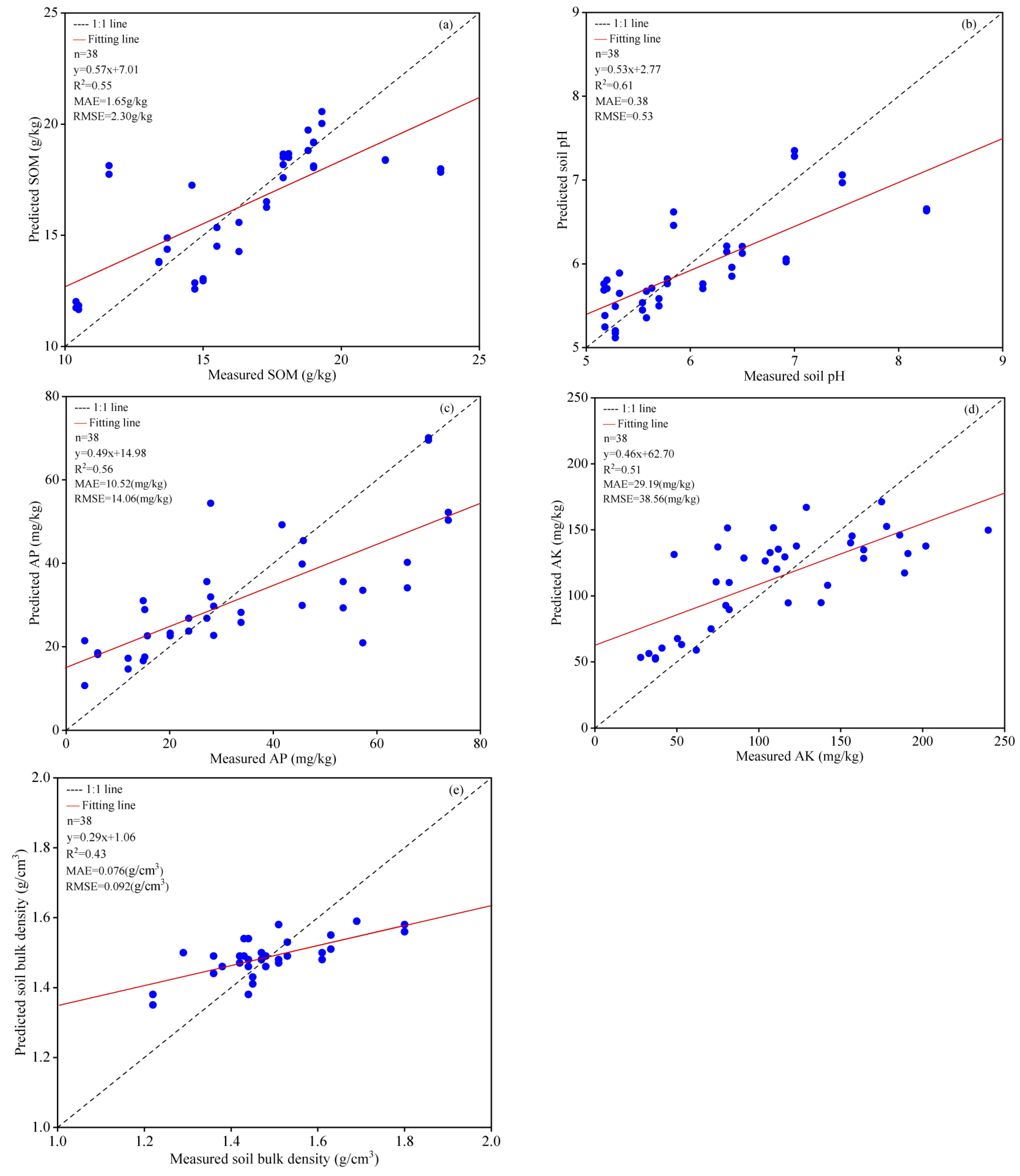
3.1. Accuracy Evaluation of Machine Learning Model

Figure 3 shows the optimal prediction results of SOM, soil pH, AP, AK and SBD. The RF model had the highest accuracy in predicting SOM, soil pH and AK, with R2 values of 0.55, 0.61 and 0.51, RMSE values of 2.30 g/kg, 0.53 and 38.56 mg/kg and MAE values of 1.65 g/kg, 0.38 and 29.19 mg/kg, respectively. The AdaBoost model had the highest accuracy in predicting AP and SBD, with R2 values of 0.56 and 0.43, RMSE values of 14.56 mg/kg and 0.076 g/cm³ and MAE values of 10.52 mg/kg and 0.092 g/cm³, respectively.

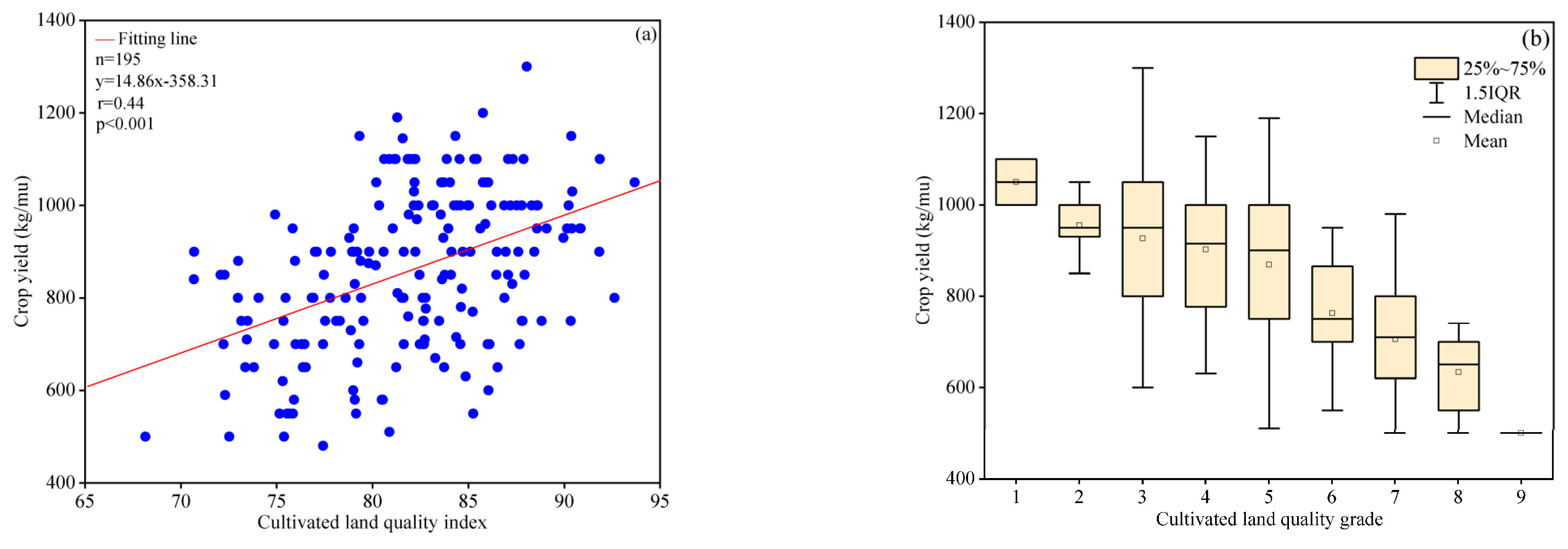
3.2. Correlation between CLQ and Crop Yield

Figure 4a shows the correlation between crop yield and CLQ index. The Pearson correlation coefficient (r) was 0.44, p < 0.001, indicating that there was a significant positive correlation between the two. Figure 4b shows the statistical analysis results of crop yield under different CLQ grades. The results showed that the higher the CLQ index, the higher the CLQ grade and the higher the crop yield, which indicated the reliability of CLQ evaluation results.

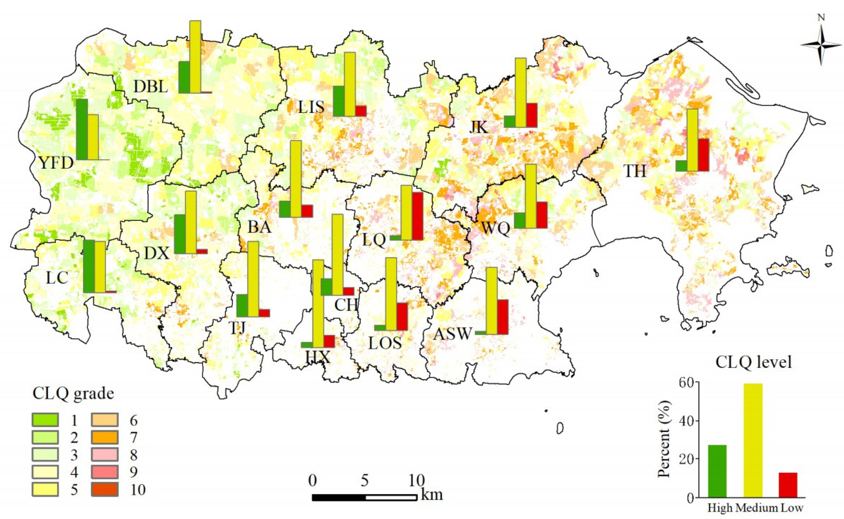
3.3. Spatial Patterns of CLQ

The area of CLQ grade 4 in Jimo district was the largest, with an area of 22,267.29 hm², accounting for 28.42%. The area of CLQ grade 5, 3 and 6 was more than 10%. The area of high-, medium- and low-quality accounted for 27.43%, 59.37% and 13.20%, respectively, indicating that the cultivated land in Jimo district was mainly of medium quality. The average index of CLQ in the study area was 82.14. The average grade of CLQ was 4.48 (

Table 7. Areas and percents of different quality grades of cultivated land in Jimo district.

CLQ grade		Area (hm2)	Precent (%)
High-quality	1	2344.62	2.99
	2	6110.55	7.80
	3	13,034.11	16.64
Medium-quality	4	22,267.29	28.42
	5	14,026.51	17.91
	6	10,214.59	13.04
Low-quality	7	6489.59	8.28
	8	3286.94	4.20
	9	528.06	0.67
	10	35.65	0.05
Total		78,337.91	100
Average CLQ index		82.14
Average CLQ grade		4.48

).

The cultivated land with high quality was distributed in the western part of the study area. The cultivated land in the eastern and central parts was of low quality (Figure 5). Cultivated land of medium quality was widely distributed throughout the Jimo district. There are obvious differences in the quality of cultivated land among different towns. YFD town had the highest CLQ index (86.41), and its CLQ grade was 3.12. The CLQ index of LC, DX, DBL and TJ towns was higher than the average value of the study area, indicating that the CLQ in these areas was good. LQ town had the lowest CLQ index (77.42), and its CLQ grade was 5.99. These things considered, ASW, TH, LOS, JK and WQ towns had a lower CLQ index, indicating that the CLQ in these areas was poor.

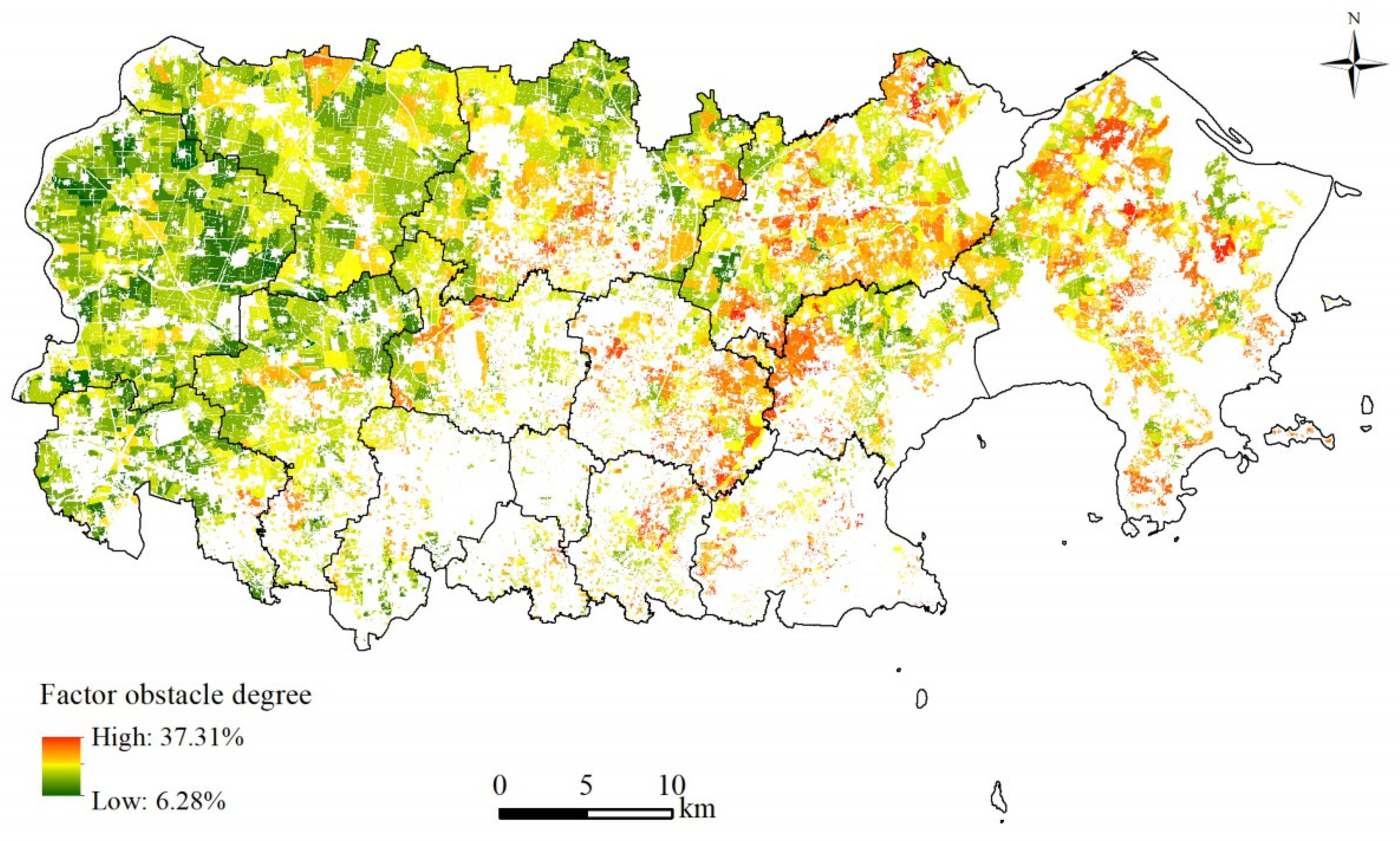
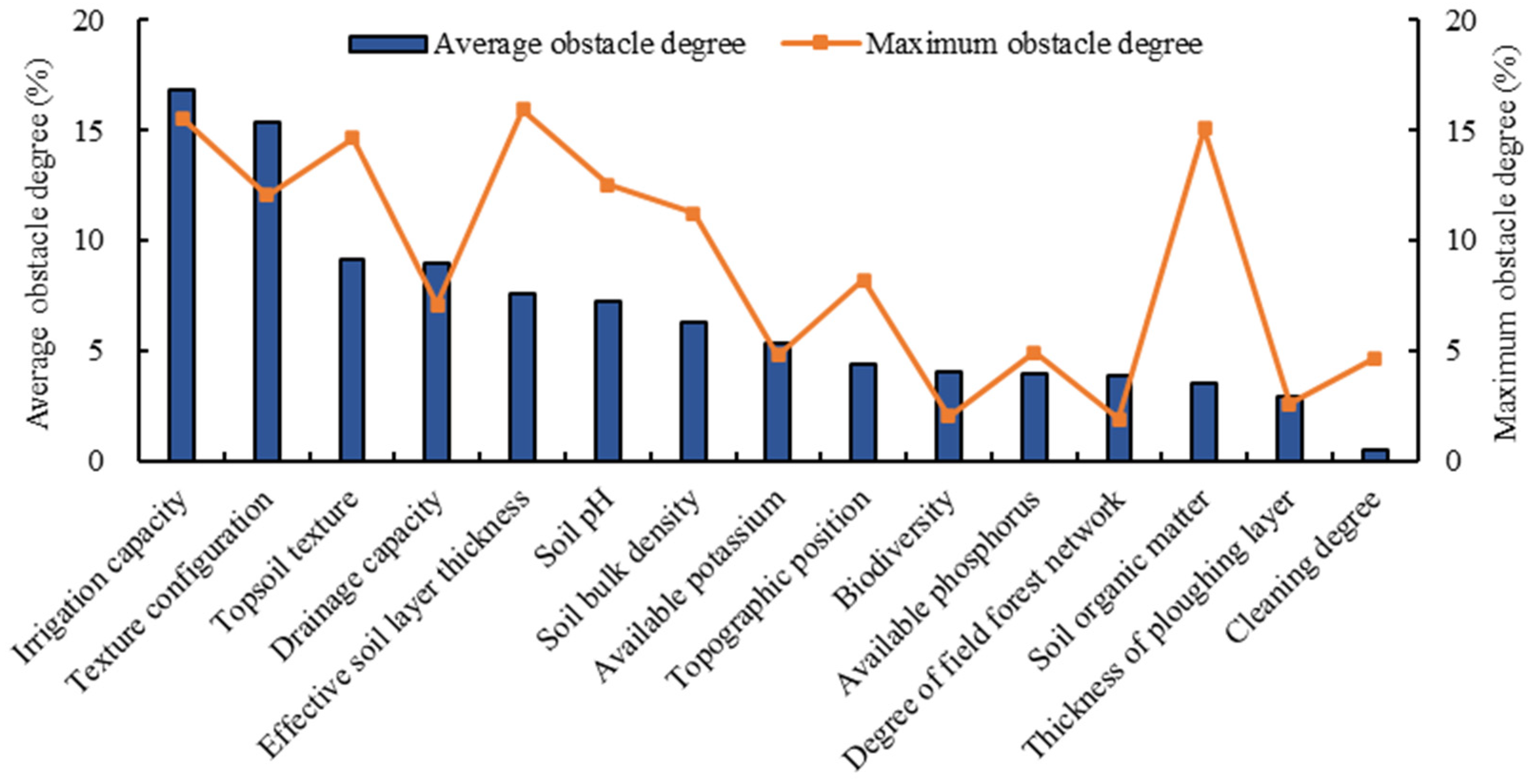
3.4. Obstacle Factors of CLQ

The spatial distribution of CLQ factor obstacle degree is shown in Figure 6. The obstacle factor degree of CLQ in the study area ranged from 6.28% to 37.31%, with an average of 18.58%. The factor obstacle degree of cultivated land in the western part was obviously lower than that in the central and eastern parts. There was a good spatial consistency between factor obstacle degree and CLQ evaluation results, indicating the CLQ was better in the area with a lower factor obstacle degree.

It was found that irrigation capacity and texture configuration were the biggest obstacle factors affecting the CLQ in Jimo district, and the average obstacle degrees were 16.85% and 15.34%, respectively (Figure 7). Although the average obstacle degrees of some indicators were small, their maximum obstacle degrees were large. For example, the maximum obstacle degrees of effective soil layer thickness, SOM and topsoil texture were more than 15% (Figure 7). To further improve the CLQ in the study area, the evaluation indicators with higher average and maximum obstacle degrees should be paid more attention.

4. Discussion

4.1. CLQ Evaluation System Based on National Standard

The intension of CLQ is complex and varied [56,57]. CLQ has developed from a single factor in the early stage to a comprehensive concept based on multiple factors [10,13,58]. However, it is not uniform across the globe at present, so there is no comparison among the results due to inconsistent definitions [16,55]. The Ministry of Agriculture and Rural Affairs of the People’s Republic of China first put forward the authoritative intension of CLQ [30]. It covered multiple factors such as cultivated land site conditions, physicochemical properties, nutrient status, soil environment, farmland infrastructure and human management and utilization and can fully characterize the comprehensive characteristics of CLQ [2,20]. Therefore, this study took this as the standard to construct the CLQ evaluation system suitable for the study area.

Indicator selection is the core of CLQ evaluation. Previous studies found that hundreds of indicators were used to evaluate the CLQ by the bibliometric and induction methods, and 65 indicators were frequently used. SOM, soil pH, effective soil layer thickness, irrigation capacity, drainage capacity and slope were selected most frequently [43]. It could be seen that the selection of indicators in previous studies focused on reflecting the physicochemical properties and nutrient status of cultivated soil and field management, while the indicators representing soil health or cultivated ecological environment were rarely applied [19,41]. In the “Cultivated Land Quality Grade” (GB/T 33469-2016) [30], based on regional division and following the principle of combining basic and regional complementarity, the selected indicators are more comprehensive, representative and less correlated with each other [18,20,59]. In this study, biodiversity and cleaning degree were selected to characterize the ecological environment of cultivated land as improvements. Thus, the CLQ evaluation system constructed was more comprehensive and rational.

4.2. CLQ Evaluation Method Based on Multi-Temporal Remote Sensing and Machine Learning Models

Appropriate methods can significantly improve the reliability and efficiency of CLQ evaluation. The traditional methods of acquiring CLQ data mainly rely on field investigation, which was inefficient and could not meet the requirements of rapid and dynamic monitoring of CLQ in large areas [33,60,61]. Remote sensing technology can quickly obtain abundant CLQ monitoring data by virtue of its strong timeliness, wide coverage and convenient data acquisition, which can effectively make up for the shortcomings of traditional methods [11,62]. In this study, Sentinel-2 image data with three consecutive periods of high time resolution (5 days) were used to quickly obtain key information of CLQ, which made the evaluation results with good timeliness.

Many studies showed that environmental variables around soil samples were closely related to soil properties, and the estimation accuracy of CLQ can be improved significantly by selecting appropriate environmental variables [47,49,50]. Through feature importance evaluation, this study found that remote sensing information (such as red, green and near-infrared band reflectance), climatic conditions (such as MAP, RH and EVA), terrain characteristics, soil attributes and cultivated land type were important environmental variables for predicting the CLQ in the study area. These important environmental variables can better characterize the spatial pattern of CLQ.

To obtain reliable evaluation results, we used three machine learning models to carry out a comparative study. The results showed that the RF model can predict SOM, soil pH and AK more accurately, while the AdaBoost model had the best performance in predicting AP and SBD. The performance of the RF model depends on the prediction accuracy of a single decision tree and the correlation among many decision trees [63]. Considering this, RF models can use missing training sample data to evaluate model performance, which can significantly improve the prediction accuracy [37]. The AdaBoost model can obtain high prediction accuracy by generating several weak learners and integrating them to form a strong learner [64]. To prevent overfitting of the machine learning models, we optimized the model parameters using GridSearch and ten-fold cross-validation.

4.3. Improving Measures and Policy Implications of CLQ

The diagnosis results of obstacle factors can help put forward targeted measures or policy suggestions for improving CLQ [2,18,20]. In this study, the diagnostic results of obstacle factors showed that irrigation capacity, texture configuration, topsoil texture, effective soil layer thickness and SOM content were the main limiting factors affecting the CLQ in the study area (Figure 7).

The cultivated land type in Jimo district was mainly dry land. More than 60% of cultivated land with irrigation capacity grades of basically satisfied and not satisfied needs to be further improved. The irrigation capacity is mainly affected by the construction of irrigation water conservancy projects, irrigation storage capacity and effective utilization coefficient of irrigation water [43,44]. Strengthening the construction of water conservancy facilities can regulate the utilization of irrigation water, so as to improve the irrigation conditions [65]. Irrigation water storage is a guarantee for the irrigation capacity [66]. However, due to over-exploitation of water resources, the amount of water available for irrigation has decreased significantly in recent years [67]. Therefore, improving the effective utilization coefficient of irrigation water is an important way to improve the irrigation capacity of cultivated land [44]. Based on physiological characteristics of crops, calculating accurate crop water requirement, formulating scientific irrigation plan and adapting sprinkling irrigation or drip irrigation can improve the irrigation capacity of cultivated land [68,69].

Organic matter is the key to improve soil structure [70]. Adding decomposed compost or other organic matter can increase the soil’s aggregate structure and porosity [71]. Adopting a reasonable fertilization strategy and the correct fertilization method can promote SOM content and microbial activity [72]. The frequency of tillage should be minimized, as over-tillage can damage the soil structure and lead to soil compaction [73]. Mulch such as straw should be used to help reduce evaporation and water loss from the soil and to provide a protective layer to prevent soil weathering and hardening [74]. In addition, the application of soil amendments can help restore soil structure and permeability, which can provide a better growing environment for crops [75]. Deep tillage of loose soil can improve the thickness of the effective soil layer without damaging the soil structure [76]. The effective measures to increase the SOM content include increasing the application of organic fertilizer, adding biochar and planting green fertilizer [77].

In terms of cultivated land protection policy, well-facilitated farmland construction is a strategic decision to ensure food security, and its construction contents include soil reclamation, land consolidation, infrastructure construction (such as irrigation and drainage ditches and field roads) and ecological environmental protection [4,9,10]. By the end of 2022, Jimo district built 53,480 hectares of well-facilitated farmland, accounting for about 70 percent of the total cultivated land area (http://www.jimo.gov.cn/) (accessed on 7 October 2023). The established well-facilitated farmland greatly improved the field infrastructure, agricultural production conditions, ecological environment and comprehensive grain production capacity [8,19]. Therefore, it should be suggested to continue to vigorously promote the construction of well-facilitated farmland, which can effectively overcome the main obstacle factors and further improve CLQ in Jimo district.

4.4. Limitations and Future Work

In recent years, deep learning models have also been applied to CLQ evaluation [78,79]. Compared with machine learning, deep learning models require more measured soil data and explanatory variables to achieve higher accuracy [80]. However, the layout of soil sampling points, data collection and indicator measurement are time-consuming and laborious, which limit their application in a large monitoring range [2]. Therefore, it is necessary to further carry out the comparative study of machine learning and deep learning models, which is conducive to the construction of a prediction model with high accuracy and universality. Meanwhile, big data cloud platforms, such as Google Earth Engine, should be adopted to improve the efficiency of CLQ evaluation.

CLQ has obvious spatial heterogeneity. According to the “Cultivated Land Quality Grade” (GB/T33469-2016) [30], China’s cultivated land is divided into nine regions. This study took Jimo district as a case study to explore the feasibility of evaluating CLQ with multi-temporal remote sensing data and machine learning models. In the future, we will apply the proposed method to other regions to evaluate its transferability.

5. Conclusions

According to China’s national standard “Cultivated Land Quality Grade” (GB/T 33469-2016), 15 indicators were selected from five aspects, including site condition, environmental condition, physicochemical property, nutrient status and field management, to construct a unified county-level CLQ evaluation system. We used multi-temporal remote sensing data, machine learning models, comprehensive index method and obstacle factor diagnosis model to reveal the spatial patterns of CLQ in Jimo district and identify the main limiting factors. The results showed that the CLQ evaluation based on multi-temporal remote sensing and machine learning model was efficient and reliable. The proportions of cultivated land of high-, medium- and poor-quality were 27.43%, 59.37% and 13.20%, respectively. CLQ in the western part of Jimo district is better, while it is worse in the eastern and central parts. Irrigation capacity, texture configuration, effective soil layer thickness and SOM were the main limiting factors. Accordingly, some targeted measures and policies were suggested, such as strengthening the construction of farmland water conservancy facilities, increasing the application of organic fertilizer, green fertilizer and biochar, deep ploughing of soil and continuing to vigorously build well-facilitated farmland.

References

1. Foley, J.A.; Ramankutty, N.; Brauman, K.A.; Cassidy, E.S.; Gerber, J.S.; Johnston, M.; Mueller, N.D.; Ray, D.K.; West, P.C.; Balzer, C. Solutions for a cultivated planet. Nature 2011, 478, 337. [Google Scholar] [CrossRef] [PubMed]
2. Zhao, C.; Zhou, Y.; Jiang, J.H.; Xiao, P.N.; Wu, H. Spatial characteristics of cultivated land quality accounting for ecological environmental condition: A case study in hilly area of northern Hubei province, China. Sci. Total Environ. 2021, 774, 145765. [Google Scholar] [CrossRef]
3. Morri, E.; Santolini, R. Ecosystem services valuation for the sustainable land use management by nature-based solution (NbS) in the common agricultural policy actions: A case study on the foglia river basin (marche region, Italy). Land 2022, 11, 57. [Google Scholar] [CrossRef]
4. Song, W.; Zhang, H.Z.; Zhao, R.; Wu, K.N.; Li, X.J.; Niu, B.B.; Li, J.Y. Study on cultivated land quality evaluation from the perspective of farmland ecosystems. Ecol. Indic. 2022, 139, 108959. [Google Scholar] [CrossRef]
5. Kong, X.B. China must protect high-quality arable land. Nature 2014, 506, 7. [Google Scholar] [CrossRef]
6. Li, W.; Wang, D.; Li, Y.; Zhu, Y.; Wang, J.; Ma, J. A multi-faceted, location-specific assessment of land degradation threats to peri-urban agriculture at a traditional grain base in northeastern China. J. Environ. Manag. 2020, 271, 111000. [Google Scholar] [CrossRef]
7. Viana, C.M.; Freire, D.; Abrantes, P.; Rocha, J.; Pereira, P. Agricultural land systems importance for supporting food security and sustainable development goals: A systematic review. Sci. Total Environ. 2022, 806, 150718. [Google Scholar] [CrossRef]
8. Shi, Y.Y.; Duan, W.K.; Fleskens, L.; Li, M.; Hao, J.M. Study on evaluation of regional cultivated land quality based on resource asset-capital attributes and its spatial mechanism. Appl. Geogr. 2020, 125, 102284. [Google Scholar] [CrossRef]
9. Gong, Y.; Zhang, Y.; Chen, Y. The impact of high-standard farmland construction policy on grain quality from the perspectives of technology adoption and cultivated land quality. Agriculture 2023, 13, 1702. [Google Scholar] [CrossRef]
10. Liu, L.M.; Zhou, D.; Chang, X.; Lin, Z.L. A new grading system for evaluating China’s cultivated land quality. Land Degrad. Dev. 2020, 31, 1482–1501. [Google Scholar] [CrossRef]
11. Liu, H.; Wang, Y.; Sang, L.; Zhao, C.; Hu, T.; Liu, H.; Zhang, Z.; Wang, S.; Miao, S.; Ju, Z. Evaluation of spatiotemporal changes in cropland quantity and quality with multi-source remote sensing. Land 2023, 12, 1764. [Google Scholar] [CrossRef]
12. Kang, L.; Zhao, R.; Wu, K.; Huang, Q.; Zhang, S. Impacts of farming layer constructions on cultivated land quality under the cultivated land balance policy. Agronomy 2021, 11, 2403. [Google Scholar] [CrossRef]
13. Miao, X.R.; Li, Z.H.; Wang, M.Y.; Mei, J.; Chen, J. Measurement of cultivated land ecosystem resilience in black soil region of Northeast China under the background of cultivated land protection policy in China: Case study of Qiqihar City. J. Clean. Prod. 2024, 434, 140141. [Google Scholar] [CrossRef]
14. Ye, S.J.; Ren, S.Y.; Song, C.Q.; Du, Z.B.; Wang, K.X.; Du, B.; Cheng, F.; Zhu, D.H. Spatial pattern of cultivated land fragmentation in mainland China: Characteristics, dominant factors, and countermeasures. Land Use Policy 2024, 139, 107070. [Google Scholar] [CrossRef]
15. Wang, N.; Zu, J.; Li, M.; Zhang, J.Y.; Hao, J.M. Spatial zoning of cultivated land in Shandong province based on the trinity of quantity, quality, and ecology. Sustainability 2020, 12, 1849. [Google Scholar] [CrossRef]
16. Li, Q.; Guo, W.; Sun, X.; Yang, A.; Qu, S.; Chi, W. The differentiation in cultivated land quality between modern agricultural areas and traditional agricultural areas: Evidence from Northeast China. Land 2021, 10, 842. [Google Scholar] [CrossRef]
17. Chen, Y.; Zhu, M.; Lu, J.; Zhou, Q.; Ma, W. Evaluation of ecological city and analysis of obstacle factors under the background of high-quality development: Taking cities in the Yellow River Basin as examples. Ecol. Indic. 2020, 118, 106771. [Google Scholar] [CrossRef]
18. Tang, M.M.; Wang, C.T.; Ying, C.Y.; Mei, S.; Tong, T.; Ma, Y.H.; Wang, Q. Research on cultivated land quality restriction factors based on cultivated land quality level evaluation. Sustainability 2023, 15, 7567. [Google Scholar] [CrossRef]
19. Duan, D.D.; Sun, X.; Liang, S.F.; Sun, J.; Fan, L.L.; Chen, H.; Xia, L.; Zhao, F.; Yang, W.Q.; Yang, P. Spatiotemporal patterns of cultivated land quality integrated with multi-source remote sensing: A case study of Guangzhou, China. Remote Sens. 2022, 14, 1250. [Google Scholar] [CrossRef]
20. Sun, X.; Li, Q.; Kong, X.; Cai, W.; Zhang, B.; Lei, M. Spatial characteristics and obstacle factors of cultivated land quality in an intensive agricultural region of the North China Plain. Land 2023, 12, 1552. [Google Scholar] [CrossRef]
21. Mamehpour, N.; Rezapour, S.; Ghaemian, N. Quantitative assessment of soil quality indices for urban croplands in acalcareous semi-arid ecosystem. Geoderma 2021, 382, 114781. [Google Scholar] [CrossRef]
22. Damiba, W.A.F.; Gathenyab, J.M.; Raude, J.M.; Home, P.G. Soil quality index (SQI) for evaluating the sustainability status of Kakia-Esamburmbur catchment under three different land use types in Narok County, Kenya. Heliyon 2024, 10, e25611. [Google Scholar] [CrossRef] [PubMed]
23. Iheshiulo, E.M.A.; Larney, F.; Hernandez-Ramirez, G.; Luce, M.S.; Chau, H.W.; Liu, K. Quantitative evaluation of soil health based on a minimum dataset under various short-term crop rotations on the Canadian prairies. Sci. Total Environ. 2024, 935, 173335. [Google Scholar] [CrossRef] [PubMed]
24. Ma, J.N.; Zhang, C.; Yun, W.J.; Lv, Y.H.; Chen, W.L.; Zhu, D.H. The temporal analysis of regional cultivated land productivity with GPP based on 2000–2018 MODIS data. Sustainability 2020, 12, 411. [Google Scholar] [CrossRef]
25. Duan, D.D.; Sun, X.; Wang, C.; Zha, Y.; Yu, Q.; Yang, P. A remote sensing approach to estimating cropland sustainability in the lateritic red soil region of China. Remote Sens. 2024, 16, 1069. [Google Scholar] [CrossRef]
26. GB/T28407-2012; Regulation for Gradation on Agriculture Land Quality. Ministry of Natural Resources of People’s Republic of China: Beijing, China, 2012. Available online: https://max.book118.com/html/2019/1113/6031221051002123.shtm (accessed on 24 July 2024). (In Chinese)
27. GB/T15618-2018; Soil Environmental Quality—Risk Control Standard for Soil Contamination of Agricultural Land. Ministry of Ecology and Environment of People’s Republic of China: Beijing, China, 2018. Available online: https://www.doc88.com/p-0791745054055.html (accessed on 24 July 2024). (In Chinese)
28. NY/ T1634-2008; Rules for Soil Quality Survey and Assessment. Ministry of Agriculture and Rural Affairs of People’s Republic of China: Beijing, China, 2008. Available online: https://www.doc88.com/p-5701003429128.html (accessed on 24 July 2024). (In Chinese)
29. Methods for Investigation, Monitoring and Evaluation of Cultivated Land Quality. Ministry of Agriculture and Rural Affairs of People’s Republic of China: 2016. Available online: https://www.gov.cn/gongbao/content/2016/content_5106203.htm (accessed on 24 July 2024). (In Chinese)
30. GB/ T33469-2016; Cultivated Land Quality Grade. Ministry of Agriculture and Rural Affairs of People’s Republic of China: Beijing, China, 2016. Available online: https://www.doc88.com/p-64159432458690.html (accessed on 24 July 2024). (In Chinese)
31. Li, T.K.; Liu, Y.; Lin, S.J.; Liu, Y.Z.; Xie, Y.F. Soil pollution management in China: A brief introduction. Sustainability 2019, 11, 556. [Google Scholar] [CrossRef]
32. Zhou, W.; Zhao, L.; Hu, Y.M.; Liu, Z.H.; Wang, L.; Ye, C.D.; Mao, X.Y.; Xie, X. Cultivated land quality evaluated using the RNN algorithm based on multisource data. Remote Sens. 2022, 14, 6014. [Google Scholar] [CrossRef]
33. Xia, Z.Q.; Peng, Y.P.; Liu, S.S.; Liu, Z.H.; Wang, G.X.; Zhu, A.X.; Hu, Y.M. The optimal image date selection for evaluating cultivated land quality based on Gaofen-1 images. Sensors 2019, 19, 4937. [Google Scholar] [CrossRef]
34. Tang, M.M.; Wang, Q.; Mei, S.; Ying, C.; Gao, Z.; Ma, Y.; Hu, H. Research on the inversion model of cultivated land quality using high-resolution remote sensing data. Agronomy 2023, 13, 2871. [Google Scholar] [CrossRef]
35. Were, K.; Bui, D.T.; Dick, Ø.B.; Singh, B.R. A comparative assessment of support vector regression, artificial neural networks, and random forests for predicting and mapping soil organic carbon stocks across an Afromontane landscape. Ecol. Indic. 2015, 52, 394–403. [Google Scholar] [CrossRef]
36. Han, Y.; Dan, Y.; Ye, Y.C.; Guo, X.; Liu, S.Y. Response of spatiotemporal variability in soil pH and associated influencing factors to land use change in a red soil hilly region in southern China. Catena 2022, 212, 106074. [Google Scholar] [CrossRef]
37. Chen, D.; Chang, N.J.; Xiao, J.F. Mapping dynamics of soil organic matter in croplands with MODIS data and machine learning algorithms. Sci. Total Environ. 2019, 669, 844–855. [Google Scholar] [CrossRef]
38. Kumar, S.; Lal, R. Mapping the organic carbon stocks of surface soils using local spatial interpolator. J. Environ. Monit. 2011, 13, 3128–3135. [Google Scholar] [CrossRef] [PubMed]
39. Somarathna, P.D.S.N.; Malone, B.P.; Minasny, B. Mapping soil organic carbon content over New South Wales, Australia using local regression kriging. Geoderma Reg. 2016, 7, 38–48. [Google Scholar] [CrossRef]
40. Yuan, X.F.; Shao, Y.J.; Li, Y.H.; Liu, Y.S.; Wang, Y.S.; Wei, X.D.; Wang, X.F.; Zhao, Y.H. Cultivated land quality improvement to promote revitalization of sandy rural areas along the Great Wall in northern Shaanxi Province, China. J. Rural Stud. 2022, 93, 367–374. [Google Scholar] [CrossRef]
41. Dai, F.Q.; Lv, Z.Q.; Liu, G.C. Assessing soil quality for sustainable cropland management based on factor analysis and fuzzy Sets: A case study in the Lhasa River Valley, Tibetan Plateau. Sustainability 2018, 10, 3477. [Google Scholar] [CrossRef]
42. He, Y.; Song, X.; Li, X.; Gao, Y.; Yang, J.; Chen, J.; Cai, C. Spatial Properties of Soil Physical Quality Index in Black Soil Croplands under Permanent Gully Erosion. Land 2023, 12, 1641. [Google Scholar] [CrossRef]
43. Duan, D.D. Remote Sensing Evaluation of Cultivated Land Quality and Its Spatiotemporal Characteristics Based on Multi-Source Data; Chinese Academy of Agricultural Sciences: Beijing, China, 2022. [Google Scholar] [CrossRef]
44. Li, X.R.; Jiang, W.L.; Duan, D.D. Spatiotemporal analysis of irrigation water use coefficients in China. J. Environ. Manag. 2020, 262, 110242. [Google Scholar] [CrossRef]
45. Zhao, R.; Wu, K.N.; Li, X.L.; Gao, N.; Yu, M.M. Discussion on the unified survey and evaluation of cultivated land quality at county scale for China’s 3rd National Land Survey: A case study of Wen county, Henan Province. Sustainability 2021, 13, 2513. [Google Scholar] [CrossRef]
46. Mahjenabadi, V.A.J.; Mousavi, S.R.; Rahmani, A.; Karami, A.; Rahmani, H.A.; Khavazi, K.; Rezaei, M. Digital mapping of soil biological properties and wheat yield using remotely sensed, soil chemical data and machine learning approaches. Comput. Electron. Agric. 2022, 197, 106978. [Google Scholar] [CrossRef]
47. Lu, Q.K.; Tian, S.; Wei, L.F. Digital mapping of soil pH and carbonates at the European scale using environmental variables and machine learning. Sci. Total Environ. 2023, 856, 159171. [Google Scholar] [CrossRef] [PubMed]
48. Estévez, V.; Mattbäck, S.; Boman, A.; Liwata-Kenttälǎ, P.; Björk, K.M.; Österholm, P. Acid sulfate soil mapping in western Finland: How to work with imbalanced datasets and machine learning. Geoderma 2024, 447, 116916. [Google Scholar] [CrossRef]
49. Bogunovic, I.; Trevisani, S.; Pereira, P.; Vukadinovic, V. Mapping soil organic matter in the Baranja region (Croatia): Geological and anthropic forcing parameters. Sci. Total Environ. 2018, 643, 335–345. [Google Scholar] [CrossRef] [PubMed]
50. Mponela, P.; Snapp, S.; Villamor, G.B.; Tamene, L.; Le, Q.B.; Borgemeister, C. Digital soil mapping of nitrogen, phosphorus, potassium, organic carbon and their crop response thresholds in smallholder managed escarpments of Malawi. Sci. Total Environ. 2020, 124, 102299. [Google Scholar] [CrossRef]
51. Klaus, V.H.; Schaub, S.; Séchaud, R.; Fabian, Y.; Jeanneretc, P.; Liüischer, A.; Huguenin-Elie, O. Upscaling of ecosystem service and biodiversity indicators from field to farm to inform agri-environmental decision- and policy-making. Ecol. Indic. 2024, 163, 112104. [Google Scholar] [CrossRef]
52. Zhao, J.Q.; Yu, L.; Newbold, T.; Shen, X.L.; Liu, X.X.; Hua, F.Y.; Kanniah, K.; Ma, K.P. Biodiversity responses to agricultural practices in cropland and natural habitats. Sci. Total Environ. 2024, 922, 171296. [Google Scholar] [CrossRef]
53. Gupta, K.; Satyam, N.; Segoni, S. A comparative study of empirical and machine learning approaches for soil thickness mapping in the Joshimath region (India). Catena 2024, 241, 108024. [Google Scholar] [CrossRef]
54. Fabian, L.; Chandrashekhar, B.; Olena, D.; Elisabeth, F.; Akmal, A.; Alejandra, N.V.; Francois, W. Regional-scale monitoring of cropland intensity and productivity with multi-source satellite image time series. GISci. Remote Sens. 2018, 55, 539–567. [Google Scholar] [CrossRef]
55. Zhang, R.Q.; Li, P.H.; Xu, L.P.; Zhong, S.; Wei, H. An integrated accounting system of quantity, quality and value for assessing cultivated land resource assets: A case study in Xinjiang, China. Glob. Ecol. Conserv. 2022, 36, e02115. [Google Scholar] [CrossRef]
56. Danso, I.; Webber, H.; Bourgault, M. Crop management adaptations to improve and stabilize crop yields under low-yielding conditions in the Sudan Savanna of West Africa. Eur. J. Agron. 2018, 101, 1–9. [Google Scholar] [CrossRef]
57. Obade, V.P. Integrating management information with soil quality dynamics to monitor agricultural productivity. Sci. Total Environ. 2019, 651, 2036–2043. [Google Scholar] [CrossRef] [PubMed]
58. Bünemann, E.K.; Bongiorno, G.; Bai, Z.G. Soil quality—A critical review. Soil. Biol. Biochem. 2018, 120, 105–125. [Google Scholar] [CrossRef]
59. Wang, Z.; Fei, X.; Sheng, M.; Xiao, R. Exploring the spatial-temporal variation in cultivated land quality and influential factors in the lower reaches of the Yangtze River from 2017 to 2020. Land 2023, 12, 322. [Google Scholar] [CrossRef]
60. Liu, S.S.; Peng, Y.P.; Xia, Z.Q.; Hu, Y.M.; Wang, G.X.; Zhu, A.X.; Liu, Z.H. The Ga-Bpnn-Based evaluation of cultivated land quality on the PSR framework using Gaofen-1 satellite data. Sensors 2019, 19, 5127. [Google Scholar] [CrossRef]
61. Li, Y.; Chang, C.; Wang, Z.; Qi, G.; Dong, C.; Zhao, G. Upscaling remote sensing inversion model of wheat field cultivated land quality in the Huang-Huai-Hai agricultural region, China. Remote Sens. 2021, 13, 5095. [Google Scholar] [CrossRef]
62. Peterson, K.T.; Sagan, V.; Sloan, J.J. Deep learning-based water quality estimation and anomaly detection using Landsat-8/Sentinel-2 virtual constellation and cloud computing. GISci. Remote Sens. 2020, 57, 510–525. [Google Scholar] [CrossRef]
63. Hateffard, F.; Steinbuch, L.; Heuvelink, G.B.M. Evaluating the extrapolation potential of random forest digital soil mapping. Geoderma 2024, 441, 116740. [Google Scholar] [CrossRef]
64. Pham, B.T.; Nguyen, M.D.; Nguyen-Thoi, T.; Ho, L.S.; Koopialipoor, M.; Quoc, N.K.; Armaghani, D.J.; Le, H.V. A novel approach for classification of soils based on laboratory tests using Adaboost, Tree and ANN modeling. Transp. Geotech. 2021, 27, 100508. [Google Scholar] [CrossRef]
65. Tong, K.; Zhao, Y.j.; Wei, Y.P.; Hu, B.Q.; Deng, J.M.; Xie, Y.C. Quantifying sediment retention by high-density small water conservancy facilities under insignificant variation of water discharge in the Nanliu River Basin, Beibu Gulf. J. Hydrol-Reg. Stud. 2022, 43, 101184. [Google Scholar] [CrossRef]
66. Lankford, B.; Pringle, C.; McCosh, J.; Shabalala, M.; Hess, T.; Knox, J.W. Irrigation area, efficiency and water storage mediate the drought resilience of irrigated agriculture in a semi-arid catchment. Sci. Total Environ. 2023, 859, 160263. [Google Scholar] [CrossRef]
67. Soylu, M.E.; Bras, R.L. Quantifying and valuing irrigation in energy and water limited agroecosystems. J. Hydrol. X 2024, 22, 100169. [Google Scholar] [CrossRef]
68. Alves, R.G.; Maia, R.F.; Lima, F. Development of a Digital Twin for smart farming: Lrrigation management system for water saving. J. Clean. Prod. 2023, 388, 135920. [Google Scholar] [CrossRef]
69. Pronti, A.; Auci, S.; Berbelc, J. Water conservation and saving technologies for irrigation. A structured literature review of econometric studies on the determinants of adoption. Agric. Water Manag. 2024, 299, 108838. [Google Scholar] [CrossRef]
70. Gregory, A.S. Degradation of soil structure and soil organic matter. Encycl. Soils Environ. 2023, 3, 246–256. [Google Scholar] [CrossRef]
71. Rasa, K.; Tahtikarhu, M.M.A.; Kahära, T.; Uusitalo, R.; Mikkola, J.; Hyvaluoma, J. A large one-time addition of organic soil amendments increased soil macroporosity but did not affect intra-aggregate porosity of a clay soil. Soil Till Res. 2024, 242, 106139. [Google Scholar] [CrossRef]
72. Sun, L.; Wang, R.; Li, J.; Wang, Q.; Lyu, W.; Wang, X.L.; Cheng, K.; Mao, H.L.; Zhang, X.Q. Reasonable fertilization improves the conservation tillage benefit for soil water use and yield of rain-fed winter wheat: A case study from the Loess Plateau, China. Field Crops Res. 2019, 242, 107589. [Google Scholar] [CrossRef]
73. Karayel, D.; Sarauskis, E. Influence of tillage methods and soil crust breakers on cotton seedling emergence in silty-loam soil. Soil Till Res. 2024, 239, 106054. [Google Scholar] [CrossRef]
74. Biswal, P.; Swain, D.K.; Jha, M.K. Straw mulch with limited drip irrigation influenced soil microclimate in improving tuber yield and water productivity of potato in subtropical India. Soil Till Res. 2022, 223, 105484. [Google Scholar] [CrossRef]
75. Plaimart, J.; Acharya, K.; Mrozik, W.; Davenport, R.J.; Vinitnantharat, S.; Werner, D. Coconut husk biochar amendment enhances nutrient retention by suppressing nitrification in agricultural soil following anaerobic digestate application. Environ. Pollut. 2021, 268, 115684. [Google Scholar] [CrossRef]
76. Li, Z.J.; Liu, H.G.; Wang, T.G.; Gong, P.; Li, P.F.; Li, L.; Bai, Z.T. Deep vertical rotary tillage depths improved soil conditions and cotton yield for saline farmland in South Xinjiang. Eur. J. Agron. 2024, 156, 127166. [Google Scholar] [CrossRef]
77. Danso, F.; Agyare, W.A.; Bart-Plange, A. Benefits and costs of cultivating rice using biochar-inorganic fertilizer combinations. J. Agric. Food Res. 2023, 11, 100491. [Google Scholar] [CrossRef]
78. Padarian, J.; MINASNY, B.; Abmcbr, A. Using deep learning to predict soil properties from regional spectral data. Geoderma Reg. 2019, 16, e00198. [Google Scholar] [CrossRef]
79. Li, H.; Ju, W.L.; Song, Y.M.; Cao, Y.Y.; Yang, W.; Li, M.Z. Soil organic matter content prediction based on two-branch convolutional neural network combining image and spectral features. Comput. Electron. Agric. 2024, 217, 108561. [Google Scholar] [CrossRef]
80. Qiao, H.L.; Xiu, B.S.; Chen, H.Z.; Liu, J.Y.; Hong, S.Y. Effective prediction of soil organic matter by deep SVD concatenation using FT-NIR spectroscopy. Soil Till Res. 2022, 215, 105223. [Google Scholar] [CrossRef]
Figure 1. Summary map of the study area. (a) Geographical location of Shandong province in China, (b) geographical location of Jimo district in Shandong province, (c) terrain feature of Jimo district and (d) spatial distribution of cultivated land and soil sampling points.
Remotesensing 16 03427 g001
Figure 2. Technology roadmap.
Remotesensing 16 03427 g002
Figure 3. Optimal prediction results of CLQ evaluation indicators: (a) soil organic matter (SOM), (b) soil pH, (c) available phosphorus (AP), (d) available potassium (AK) and (e) soil bulk density (SBD).
Remotesensing 16 03427 g003
Figure 4. Relationship between crop yield, CLQ index (a) and CLQ grade (b).
Remotesensing 16 03427 g004
Figure 5. Spatial distribution of CLQ grade and level in Jimo district. DX: Daxin Street; LIS: Lingshan Street; LC: Lancun Street; TJ: Tongji Street; CH: Chaohai Street; TH: Tianheng town; JK: Jinkou town; BA: Beian Street; LOS: Longshan Street; HX: Huanxiu Street; YSD: Yifengdian town; ASW: Aoshanwei Street; DBL: Duanbolan town; LQ: Longquan Street; and WQ: Wenquan Street.
Remotesensing 16 03427 g005
Figure 6. Spatial distribution of CLQ factor obstacle degree.
Remotesensing 16 03427 g006
Figure 7. Average and maximum obstacle degrees of CLQ evaluation indicators.
Remotesensing 16 03427 g007