


Mapping Field-Level Maize Yields in Ethiopian Smallholder Systems Using Sentinel-2 Imagery

 , ,
, ,
Abstract
1. Introduction
- 1.
- How well can we map field-level yields in smallholder maize systems in Ethiopia using Sentinel-2 imagery?
- 2.
- Which vegetation index results in the highest yield prediction accuracies: the NDVI, GCVI, or MTCI?
- 3.
- Which model leads to higher prediction accuracies: multiple linear regression or random forest regression?
- 4.
- Does imputing missing values due to cloud cover improve model performance?
- 5.
- Can adding weather and soil data improve prediction accuracy compared to using only vegetation indices?
- 6.
- Is it possible to create a generalizable model that accurately estimates yields across multiple regions using limited ground data for training?
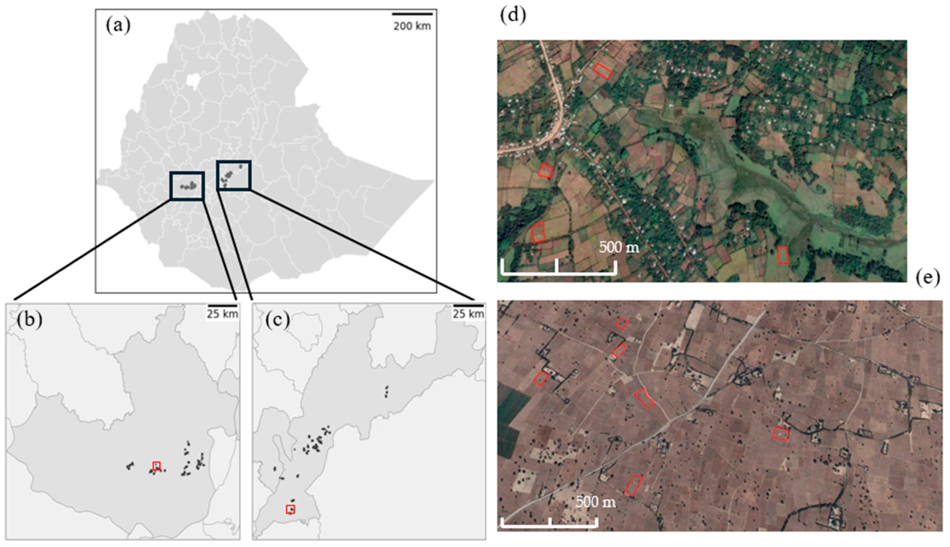
2. Study Area
3. Methods
3.1. Crop Cut Data
3.2. Sentinel-2 Imagery
3.3. Environmental Data
3.4. Model Parameterization and Validation
3.5. Comparison of Models by Sub-Region
4. Results
5. Discussion
6. Conclusions
Supplementary Materials
Author Contributions
Funding
Institutional Review Board Statement
Data Availability Statement
Conflicts of Interest
References
- Godfray, C.; Beddington, J.; Crute, I.; Haddad, L.; Lawrence, D.; Muir, J.; Pretty, J.; Robinson, S.; Toulmin, C. Food Security: The Challenge of Feeding 9 Billion People. Science 2010, 327, 812–823. [Google Scholar] [CrossRef] [PubMed]
- Tilman, D.; Balzer, C.; Hill, J.; Befort, B.L. Global food demand and the sustainable intensification of agriculture. Proc. Natl. Acad. Sci. USA 2011, 108, 20260–20264. [Google Scholar] [CrossRef] [PubMed]
- Lobell, D.B.; Cassman, K.G.; Field, C.B. Crop Yield Gaps: Their Importance, Magnitudes, and Causes. Annu. Rev. Environ. Resour. 2009, 34, 179–204. [Google Scholar] [CrossRef]
- Mueller, N.; Gerber, J.S.; Johnston, M.; Ray, D.K.; Ramankutty, N.; Foley, J.A. Closing yield gaps through nutrient and water management. Nature 2012, 490, 254–257. [Google Scholar] [CrossRef]
- Bezner Kerr, R.; Hasegawa, T.; Lasco, R.; Bhatt, I.; Deryng, D.; Farrell, A.; Gurney-Smith, H.; Ju, H.; Lluch-Cota, S.; Meza, F.; et al. Food, Fibre, and Other Ecosystem Products. In Climate Change 2022: Impacts, Adaptation and Vulnerability. Contribution of Working Group II to the Sixth Assessment Report of the Intergovernmental Panel on Climate Change; Pörtner, H.-O., Roberts, D.C., Tignor, M., Poloczanska, E.S., Mintenbeck, K., Alegría, A., Craig, M., Langsdorf, S., Löschke, S., Möller, V., et al., Eds.; Cambridge University Press: Cambridge, UK; New York, NY, USA, 2022; pp. 713–906. [Google Scholar]
- OECD/FAO. OECD-FAO Agricultural Outlook 2022–2031; OECD Publishing: Paris, France, 2022. [Google Scholar]
- Di Falco, S.; Veronesi, M.; Yesuf, M. Does adaptation to climate provide food security? A micro-perspective from Ethiopia. Am. J. Agric. Econ. 2011, 93, 829–846. [Google Scholar] [CrossRef]
- Mohamed, A. Food Security Situation in Ethiopia: A Review Study. Int. J. Health Econ. Policy 2017, 2, 86–96. [Google Scholar]
- Abate, T.; Shiferaw, B.; Menkir, A.; Wegary, D.; Kebede, Y.; Tesfaye, K.; Kassie, M.; Bogale, G.; Tadesse, B.; Keno, T. Factors that transformed maize productivity in Ethiopia. Food Sec. 2015, 7, 965–981. [Google Scholar] [CrossRef]
- Carletto, C.; Jolliffe, D.; Banerjee, R. From Tragedy to Renaissance: Improving Agricultural Data for Better Policies. J. Dev. Stu. 2013, 51, 133–148. [Google Scholar] [CrossRef]
- Paliwal, A.; Jain, M. The Accuracy of Self-Reported Crop Yield Estimates and Their Ability to Train Remote Sensing Algorithms. Front. Sustain. Food Syst. 2020, 4, 25. [Google Scholar] [CrossRef]
- Paliwal, A.; Balwinder-Singh; Poonia, S.; Jain, M. Using microsatellite data to estimate the persistence of field-level yield gaps and their drivers in smallholder systems. Sci. Rep. 2023, 13, 11170. [Google Scholar] [CrossRef]
- Jain, M.; Srivastava, A.K.; Singh, B.; Joon, R.J.; McDonald, A.; Royal, K.; Lisaius, M.C.; Lobell, D.B. Mapping Smallholder Wheat Yields and Sowing Dates Using Micro-Satellite Data. Remote Sens. 2016, 8, 860. [Google Scholar] [CrossRef]
- Azzari, G.; Jain, M.; Lobell, D. Towards fine resolution global maps of crop yields: Testing multiple methods and satellites in three countries. Remote Sens. Environ. 2017, 202, 129–141. [Google Scholar] [CrossRef]
- Sweeney, S.; Ruseva, T.; Estes, L.; Evans, T. Mapping Cropland in Smallholder-Dominated Savannas: Integrating Remote Sensing Techniques and Probabilistic Modeling. Remote Sens. 2015, 7, 15295–15317. [Google Scholar] [CrossRef]
- Jin, Z.; Azzari, G.; You, C.; Di Tommaso, S.; Aston, S.; Burke, M.; Lobell, D.B. Smallholder maize area and yield mapping at national scales with Google Earth Engine. Remote Sens. Environ. 2019, 228, 115–128. [Google Scholar] [CrossRef]
- Hunt, M.L.; Blackburn, G.A.; Carrasco, L.; Redhead, J.W.; Rowland, C.S. High resolution wheat yield mapping using Sentinel-2. Remote Sens. Environ. 2019, 233, 111410. [Google Scholar]
- Gao, F.; Zhang, X. Mapping crop phenology in near real-time using satellite remote sensing: Challenges and opportunities. J. Remote Sens. 2021, 2021, 8379391. [Google Scholar] [CrossRef]
- Zhang, L.; Zhang, Z.; Luo, Y.; Cao, J.; Xie, R.; Li, S. Integrating satellite-derived climatic and vegetation indices to predict smallholder maize yield using deep learning. Agric. For. Meteorol. 2021, 311, 108666. [Google Scholar] [CrossRef]
- Aranguren, M.; Castellon, A.; Aizpurua, A. Wheat yield estimation with NDVI values using a proximal sensing tool. Remote Sens. 2020, 12, 2749. [Google Scholar] [CrossRef]
- Johnson, D.M.; Rosales, A.; Mueller, R.; Reynolds, C.; Frantz, R.; Anyamba, A.; Pak, E.; Tucker, C. USA crop yield estimation with MODIS NDVI: Are remotely sensed models better than simple trend analysis? Remote Sens. 2021, 13, 21. [Google Scholar] [CrossRef]
- Clevers, J.G.P.W.; Gitelson, A.A. Remote estimation of crop and grass chlorophyll and nitrogen content using red-edge bands on Sentinel-2 and -3. Int. J. Appl. Earth Obs. Geoinf. 2013, 23, 344–451. [Google Scholar] [CrossRef]
- Houborg, R.; McCabe, M. A Cubesat enabled Spatio-Temporal Enhancement Method (CESTEM) utilizing Planet, Landsat and MODIS data. Remote Sens. Environ. 2018, 209, 211–226. [Google Scholar] [CrossRef]
- Nguy-Robertson, A.L.; Peng, Y.; Gitelson, A.A.; Arkebauer, T.J.; Pimstein, A.; Herrmann, I.; Karnieli, A.; Rundquist, D.C.; Bonfil, D.J. Estimating green LAI in four crops: Potential of determining optimal spectral bands for a universal algorithm. Agric. For. Meteorol. 2014, 192, 140–148. [Google Scholar] [CrossRef]
- Burke, M.; Lobell, D.B. Satellite-based assessment of yield variation and its determinants in smallholder African systems. Proc. Natl. Acad. Sci. USA 2017, 114, 2189–2194. [Google Scholar] [CrossRef] [PubMed]
- Jin, Z.; Azzari, G.; Burke, M.; Aston, S.; Lobell, D. Mapping smallholder yield heterogeneity at multiple scales in Eastern Africa. Remote Sens. 2017, 9, 931. [Google Scholar] [CrossRef]
- Lobell, D.B.; Thau, D.; Seifert, C.; Engle, E.; Little, B. A scalable satellite-based crop yield mapper. Remote Sens. Environ. 2015, 164, 324–333. [Google Scholar] [CrossRef]
- Jain, M.; Singh, B.; Srivastava, A.A.K.; Malik, R.K.; McDonald, A.J.; Lobell, D.B. Using satellite data to identify the causes of and potential solutions for yield gaps in India’s Wheat Belt. Environ. Res. Lett. 2017, 12, 094011. [Google Scholar] [CrossRef]
- Ansarifar, J.; Wang, L.; Archontoulis, S.V. An interaction regression model for crop yield prediction. Sci. Rep. 2021, 11, 17754. [Google Scholar] [CrossRef]
- Farmonov, N.; Amankulova, K.; Szatmári, J.; Urinov, J.; Narmanov, Z.; Nosirov, J.; Mucsi, L. Combining PlanetScope and Sentinel-2 images with environmental data for improved wheat yield estimation. Int. J. Digit. Earth 2023, 16, 847–867. [Google Scholar] [CrossRef]
- Sibley, A.M.; Grassini, P.; Thomas, N.E.; Cassman, K.G.; Lobell, D.B. Testing Remote Sensing Approaches for Assessing Yield Variability among Maize Fields. Agron. J. 2014, 106, 24–32. [Google Scholar] [CrossRef]
- Desloires, J.; Ienco, D.; Botrel, A. Out-of-year corn yield prediction at field-scale using Sentinel-2 satellite imagery and machine learning methods. Comput. Electron. Agric. 2023, 209, 107807. [Google Scholar] [CrossRef]
- Ray, D.; Gerber, J.; MacDonald, G.; West, P.C. Climate variation explains a third of global crop yield variability. Nat. Commun. 2015, 6, 5989. [Google Scholar] [CrossRef] [PubMed]
- Leroux, L.; Baron, C.; Zoungrana, B.; Traoré, S.B.; Lo Seen, D.; Bégué, A. Crop Monitoring Using Vegetation And Thermal Indices For Yield Estimates: Case Study Of A Rainfed Cereal In Semi-Arid West Africa. IEEE J. Sel. Top. Appl. Earth Obs. Remote Sens. 2016, 9, 347–362. [Google Scholar] [CrossRef]
- Mladenova, I.; Bolten, J.; Crow, W.; Anderson, M.; Hain, C.; Johnson, D.; Mueller, R. Intercomparison of Soil Moisture, Evaporative Stress, and Vegetation Indices for Estimating Corn and Soybean Yields Over the U.S. IEEE J. Sel. Top. Appl. Earth Obs. Remote Sens. 2017, 10, 1328–1343. [Google Scholar] [CrossRef]
- Johnson, D.M. An assessment of pre- and within-season remotely sensed variables for forecasting corn and soybean yields in the United States. Remote Sens. Environ. 2014, 141, 116–128. [Google Scholar] [CrossRef]
- Johnson, D.M.; Hsieh, W.W.; Cannon,, A.J.; Davidson, A.; Bédard, F. Crop yield forecasting on the Canadian Prairies by remotely sensed vegetation indices and machine learning methods. Agric. For. Meteorol. 2016, 218–219, 74–84. [Google Scholar] [CrossRef]
- Leroux, L.; Castets, M.; Baron, C.; Escorihuela, M.J.; Begue, A.; Lo Seen, D. Maize yield estimation in West Africa from crop process-induced combinations of multi-domain remote sensing indices. Eur. J. Agron. 2019, 108, 11–26. [Google Scholar] [CrossRef]
- Kang, Y.; Ozdogan, M.; Zhu, X.; Ye, Z.; Hain, C.; Anderson, M. Comparative assessment of environmental variables and machine learning algorithms for maize yield prediction in the US Midwest. Environ. Res. Lett. 2019, 15, 064005. [Google Scholar] [CrossRef]
- Debalke, D.B.; Abebe, J.T. Maize yield forecast using GIS and remote sensing in Kaffa Zone, South West Ethiopia. Environ. Syst. Res. 2022, 11, 1. [Google Scholar] [CrossRef]
- Guo, Z.; Chamberlin, J.; You, L. Smallholder maize yield estimation using satellite data and machine learning in Ethiopia. Crop Environ. 2023, 2, 165–174. [Google Scholar] [CrossRef]
- Hadado, T.T.; Rau, D.; Bitocchi, E.; Papa, R. Genetic diversity of barley (Hordeum vulgare L.) landraces from the central highlands of Ethiopia: Comparison between the Belg and Meher growing seasons using morphological traits. Genet. Resour. Crop Evol. 2009, 56, 1131–1148. [Google Scholar] [CrossRef]
- Wakjira, M.T.; Peleg, N.; Anghileri, D.; Molnar, D.; Alamirew, T.; Six, J.; Molnar, P. Rainfall seasonality and timing: Implications for cereal crop production in Ethiopia. Agric. For. Meteorol. 2021, 310, 108633. [Google Scholar] [CrossRef]
- Tiedeman, K.; Chamberlin, J.; Kosmowski, F.; Ayalew, H.; Sida, T.; Hijmans, R.J. Field Data Collection Methods Strongly Affect Satellite-Based Crop Yield Estimation. Remote Sens. 2022, 14, 1995. [Google Scholar] [CrossRef]
- Gillies, S. Shapely: Manipulation and Analysis of Geometric Objects. 2007. Available online: https://github.com/Toblerity/Shapely (accessed on 3 January 2024).
- Gorelick, N.; Hancher, M.; Dixon, M.; Ilyushchenko, S.; Thau, D.; Moore, R. Google Earth Engine: Planetary-scale geospatial analysis for everyone. Remote Sens. Environ. 2017, 202, 18–27. [Google Scholar] [CrossRef]
- Zupanc, A. Improving Cloud Detection with Machine Learning. Available online: https://medium.com/sentinel-hub/improving-cloud-detection-with-machine-learning-c09dc5d7cf13 (accessed on 2 January 2023).
- Rouse, J.W.; Haas, R.H.; Schell, J.A.; Deering, D.W. Monitoring Vegetation Systems in the Great Okains with ERTS. In Proceedings of the Third Earth Resources Technology Satellite-1 Symposium, Washington, DC, USA, 10–14 December 1973; Freden, S.C., Mercanti, E.P., Eds.; NASA: Washington, DC, USA, 1974. [Google Scholar]
- Gitelson, A.A.; Gritz, Y.; Merzlyak, M.N. Relationships between leaf chlorophyll content and spectral reflectance and algorithms for non-destructive chlorophyll assessment in higher plant leaves. J. Plant Physiol. 2003, 160, 271–282. [Google Scholar] [CrossRef]
- Dash, J.; Curran, P.J. The MERIS terrestrial chlorophyll index. Int. J. Remote Sens. 2004, 2523, 5403–5413. [Google Scholar] [CrossRef]
- Wan, Z. New refinements and validation of the MODIS Land-Surface Temperature/Emissivity products. Remote Sens. Environ. 2008, 112, 59–74. [Google Scholar] [CrossRef]
- Funk, C.; Peterson, P.; Landsfeld, M.; Pereros, D.; Verdin, J.; Shukla, S.; Husak, G.; Rowland, J.; Harrison, L.; Hoell, A.; et al. The climate hazards infrared precipitation with stations—A new environmental record for monitoring extremes. Sci. Data 2015, 2, 150066. [Google Scholar] [CrossRef]
- Hengl, T.; Mendes de Jesus, J.; Heuvelink, G.B.M.; Ruiperez, M.G.; Kilibarda, M.; Blagotić, A. SoilGrids250m: Global gridded soil information based on machine learning. PLoS ONE 2017, 12, 0169748. [Google Scholar] [CrossRef]
- Pedregosa, F.; Varoquaux, G.; Gramfort, A.; Michel, V.; Thirion, B.; Grisel, O.; Blondel, M.; Prettenhofer, P.; Weiss, R.; Dubourg, V. Scikit-learn: Machine learning in Python. J. Mach. Learn. Res. 2011, 12, 2825–2830. [Google Scholar]
- Breiman, L. Random Forests. Mach. Learn. 2001, 45, 5–32. [Google Scholar] [CrossRef]
- Bergstra, J.; Bengio, Y. Random Search for Hyper-Parameter Optimization. J. Mach. Learn. Res. 2012, 13, 281–305. [Google Scholar]
- Zhao, Y.; Potgieter, A.B.; Zhang, M.; Wu, B.; Hammer, G.L. Predicting wheat yield at the field scale by combining high-resolution Sentinel-2 imagery and crop modeling. Remote Sens. 2020, 12, 1024. [Google Scholar] [CrossRef]
- Jain, M.; Balwinder-Singh; Rao, P.; Srivastava, A.K.; Poonia, S.; Blesh, J.; Azzari, G.; McDonald, A.J.; Lobell, D.B. The impact of agricultural interventions can be doubled by using satellite data. Nat. Sustain. 2019, 2, 931–934. [Google Scholar] [CrossRef]
- Sellers, P.J. Canopy reflectance, photosynthesis and transpiration. Int. J. Remote Sens. 1985, 6, 1335–1372. [Google Scholar] [CrossRef]
- Dash, J.; Lankester, T.; Hubbard, S.; Curran, P.J. Signal-to-noise ratio for MTCI and NDVI time series data. In Proceedings of the 2nd MERIS/(A)ATSR User Workshop, Frascati, Italy, 22–26 September 2007. [Google Scholar]
- Gu, Y.; Wylie, B.K.; Howard, D.M.; Phuyal, K.P.; Ji, L. NDVI saturation adjustment: A new approach for improving cropland performance estimates in the Greater Platte River Basin, USA. Ecol. Indic. 2013, 30, 1–6. [Google Scholar] [CrossRef]
- Ulfa, F.; Orton, T.G.; Dang, Y.P.; Menzies, N.W. Developing and Testing Remote-Sensing Indices to Represent within-Field Variation of Wheat Yields: Assessment of the Variation Explained by Simple Models. Agronomy 2022, 12, 384. [Google Scholar] [CrossRef]
- Tucker, C.J. Asymptotic nature of grass canopy spectral reflectance. Appl. Opt. 1977, 16, 1151–1156. [Google Scholar] [CrossRef]
- Lobell, D.B.; Azzari, G.; Burke, M.; Gourlay, S.; Jin, Z.; Kilic, T.; Murray, S. Eyes in the Sky, Boots on the Ground: Assessing Satellite- and Ground-Based Approaches to Crop Yield Measurement and Analysis. Am. J. Agric. Econ. 2020, 102, 202–219. [Google Scholar] [CrossRef]
- Hengl, T.; Nussbaum, M.; Wright, N.M.; Heuvelink, G.B.M.; Graler, B. Random forest as a generic framework for predictive modeling of spatial and spatio-temporal variables. PeerJ 2018, 6, 5518. [Google Scholar] [CrossRef]
- Pede, T.; Mountrakis, G.; Shaw, S.B. Improving corn yield prediction across the US Corn Belt by replacing air temperature with daily MODIS land surface temperature. Agric. For. Meteorol. 2019, 276, 107615. [Google Scholar] [CrossRef]
- Amede, T.; Auricht, C.; Boffa, J.M.; Dixon, J.; Mallawaarachchi, T.; Rukuni, M.; Deneke, T. The Evolving Farming and Pastoral Landscapes in Ethiopia: A Farming System Framework for Investment Planning and Priority Setting; ACIAR: Canberra, Australia, 2015; ISBN 1056875700. [Google Scholar]
- Sakamoto, T. Incorporating environmental variables into a MODIS-based crop yield estimation method for United States corn and soybeans through the use of a Random Forest regression algorithm. ISPRS J. Photogramm. Remote Sens. 2020, 160, 208–228. [Google Scholar] [CrossRef]


| Band | Spectral Range (nm) | Resolution (m) |
|---|---|---|
| Green | 543–578 | 10 |
| Red | 650–680 | 10 |
| Red Edge (RE) | 690–730 | 20 |
| Near Infrared (NIR) | 760–850 | 10 |
| Vegetation Index | Formula | Reference |
|---|---|---|
| Normalized Difference Vegetation Index (NDVI) | (NIR − Red)/(NIR + Red) | Rouse et al., 1973 [48] |
| Green Chlorophyll Vegetation Index (GCVI) | (NIR/Green − 1) | Gitelson et al., 2003 [49] |
| MERIS Terrestrial Chlorophyll Index (MTCI) | (NIR − RE)/(RE − Red) | Dash & Curran, 2004 [50] |
| Region/Sub-Region | Regressor | Vegetation Index (VI) | Temporal Resolution | Coefficient of Determination (R2) | Root Mean Squared Error (RMSE) |
|---|---|---|---|---|---|
| Regional | Linear | GCVI | Monthly | 0.11 | 2057 |
| Regional | Linear | MTCI | Monthly | 0.23 | 1913 |
| Regional | Linear | NDVI | Monthly | 0.17 | 1988 |
| Regional | Random Forest | GCVI | Monthly | 0.16 | 1997 |
| Regional | Random Forest | MTCI | Monthly | 0.28 | 1846 |
| Regional | Random Forest | NDVI | Monthly | 0.09 | 2077 |
| East Shewa-Guraghe | Linear | GCVI | Biweekly | 0.35 | 1788 |
| East Shewa-Guraghe | Linear | MTCI | Biweekly | 0.49 | 1579 |
| East Shewa-Guraghe | Linear | NDVI | Biweekly | 0.34 | 1806 |
| East Shewa-Guraghe | Random Forest | GCVI | Biweekly | 0.43 | 1668 |
| East Shewa-Guraghe | Random Forest | MTCI | Biweekly | 0.5 | 1574 |
| East Shewa-Guraghe | Random Forest | NDVI | Biweekly | 0.35 | 1788 |
| East Shewa-Guraghe | Linear | GCVI | Monthly | 0.45 | 1647 |
| East Shewa-Guraghe | Linear | MTCI | Monthly | 0.47 | 1621 |
| East Shewa-Guraghe | Linear | NDVI | Monthly | 0.4 | 1716 |
| East Shewa-Guraghe | Random Forest | GCVI | Monthly | 0.4 | 1713 |
| East Shewa-Guraghe | Random Forest | MTCI | Monthly | 0.49 | 1576 |
| East Shewa-Guraghe | Random Forest | NDVI | Monthly | 0.22 | 1955 |
| Jimma | Linear | GCVI | Monthly | 0.17 | 1969 |
| Jimma | Linear | MTCI | Monthly | 0.32 | 1782 |
| Jimma | Linear | NDVI | Monthly | 0.17 | 1974 |
| Jimma | Random Forest | GCVI | Monthly | 0.19 | 1946 |
| Jimma | Random Forest | MTCI | Monthly | 0.35 | 1746 |
| Jimma | Random Forest | NDVI | Monthly | 0.02 | 2149 |
| Region/Sub-Region | Regressor | Vegetation Index (VI) | Temporal Resolution | Coefficient of Determination (R2) | Root Mean Squared Error (RMSE) |
|---|---|---|---|---|---|
| East Shewa-Guraghe | Linear | GCVI | Monthly | 0.41 | 1663 |
| East Shewa-Guraghe | Linear | MTCI | Monthly | 0.57 | 1422 |
| East Shewa-Guraghe | Linear | NDVI | Monthly | 0.33 | 1776 |
| East Shewa-Guraghe | Random Forest | GCVI | Monthly | 0.36 | 1732 |
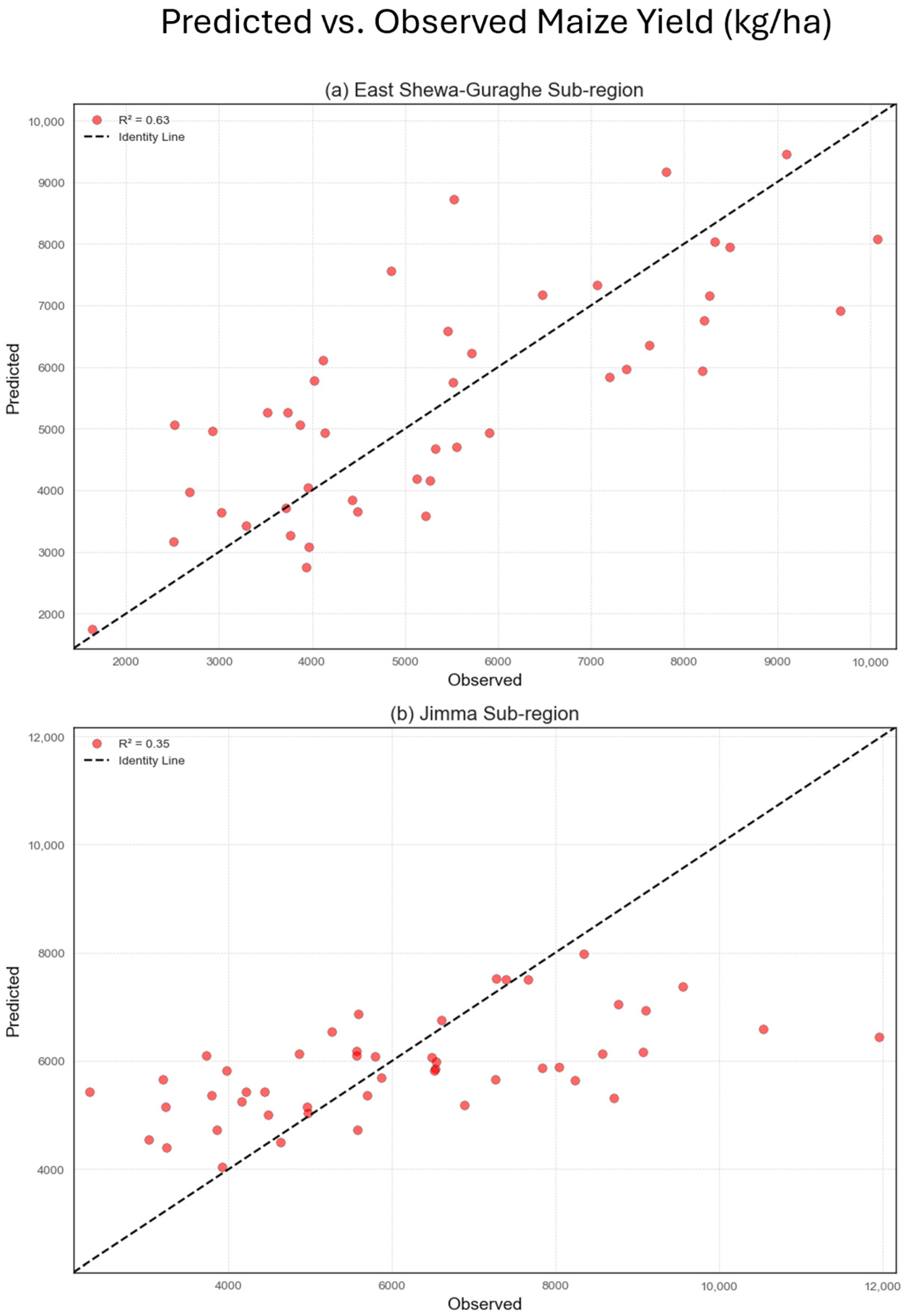
| East Shewa-Guraghe | Random Forest | MTCI | Monthly | 0.63 | 1326 |
| East Shewa-Guraghe | Random Forest | NDVI | Monthly | 0.26 | 1875 |
| Region/Sub-Region | Regressor | Vegetation Index (VI) | Temporal Resolution | Coefficient of Determination (R2) | Root Mean Squared Error (RMSE) |
|---|---|---|---|---|---|
| Regional | Linear | GCVI | Monthly | 0.11 | 2061 |
| Regional | Linear | MTCI | Monthly | 0.25 | 1894 |
| Regional | Linear | NDVI | Monthly | 0.14 | 2021 |
| Regional | Random Forest | GCVI | Monthly | 0.19 | 1966 |
| Regional | Random Forest | MTCI | Monthly | 0.33 | 1786 |
| Regional | Random Forest | NDVI | Monthly | 0.11 | 2054 |
| East Shewa-Guraghe | Linear | GCVI | Biweekly | 0.43 | 1672 |
| East Shewa-Guraghe | Linear | MTCI | Biweekly | 0.48 | 1601 |
| East Shewa-Guraghe | Linear | NDVI | Biweekly | 0.33 | 1814 |
| East Shewa-Guraghe | Random Forest | GCVI | Biweekly | 0.44 | 1654 |
| East Shewa-Guraghe | Random Forest | MTCI | Biweekly | 0.52 | 1540 |
| East Shewa-Guraghe | Random Forest | NDVI | Biweekly | 0.37 | 1753 |
| East Shewa-Guraghe | Linear | GCVI | Monthly | 0.48 | 1606 |
| East Shewa-Guraghe | Linear | MTCI | Monthly | 0.46 | 1624 |
| East Shewa-Guraghe | Linear | NDVI | Monthly | 0.35 | 1786 |
| East Shewa-Guraghe | Random Forest | GCVI | Monthly | 0.43 | 1675 |
| East Shewa-Guraghe | Random Forest | MTCI | Monthly | 0.56 | 1475 |
| East Shewa-Guraghe | Random Forest | NDVI | Monthly | 0.29 | 1870 |
| Jimma | Linear | GCVI | Monthly | 0.18 | 1961 |
| Jimma | Linear | MTCI | Monthly | 0.29 | 1828 |
| Jimma | Linear | NDVI | Monthly | 0.16 | 1988 |
| Jimma | Random Forest | GCVI | Monthly | 0.16 | 1986 |
| Jimma | Random Forest | MTCI | Monthly | 0.32 | 1789 |
| Jimma | Random Forest | NDVI | Monthly | 0.04 | 2122 |
| Training Sub-Region | Validation Sub-Region | Regressor | Vegetation Index (VI) | R2 (Training) | R2 (Validation) | RMSE (Training) | RMSE (Validation) |
|---|---|---|---|---|---|---|---|
| East Shewa-Guraghe | Jimma | Linear | MTCI | 0.47 | 0.17 | 1627 | 1791 |
| East Shewa-Guraghe | Jimma | Random Forest | MTCI | 0.49 | 0.17 | 1584 | 1791 |
| Jimma | East Shewa-Guraghe | Linear | MTCI | 0.32 | 0.36 | 1791 | 1736 |
| Jimma | East Shewa-Guraghe | Random Forest | MTCI | 0.35 | 0.30 | 1751 | 1823 |
Disclaimer/Publisher’s Note: The statements, opinions and data contained in all publications are solely those of the individual author(s) and contributor(s) and not of MDPI and/or the editor(s). MDPI and/or the editor(s) disclaim responsibility for any injury to people or property resulting from any ideas, methods, instructions or products referred to in the content. |
© 2024 by the authors. Licensee MDPI, Basel, Switzerland. This article is an open access article distributed under the terms and conditions of the Creative Commons Attribution (CC BY) license (https://creativecommons.org/licenses/by/4.0/).
Share and Cite
Mondschein, Z.; Paliwal, A.; Sida, T.S.; Chamberlin, J.; Wang, R.; Jain, M. Mapping Field-Level Maize Yields in Ethiopian Smallholder Systems Using Sentinel-2 Imagery. Remote Sens. 2024, 16, 3451. https://doi.org/10.3390/rs16183451
Mondschein Z, Paliwal A, Sida TS, Chamberlin J, Wang R, Jain M. Mapping Field-Level Maize Yields in Ethiopian Smallholder Systems Using Sentinel-2 Imagery. Remote Sensing. 2024; 16(18):3451. https://doi.org/10.3390/rs16183451
Chicago/Turabian StyleMondschein, Zachary, Ambica Paliwal, Tesfaye Shiferaw Sida, Jordan Chamberlin, Runzi Wang, and Meha Jain. 2024. "Mapping Field-Level Maize Yields in Ethiopian Smallholder Systems Using Sentinel-2 Imagery" Remote Sensing 16, no. 18: 3451. https://doi.org/10.3390/rs16183451
APA StyleMondschein, Z., Paliwal, A., Sida, T. S., Chamberlin, J., Wang, R., & Jain, M. (2024). Mapping Field-Level Maize Yields in Ethiopian Smallholder Systems Using Sentinel-2 Imagery. Remote Sensing, 16(18), 3451. https://doi.org/10.3390/rs16183451