Resource Allocation of Netted Opportunistic Array Radar for Maneuvering Target Tracking under Uncertain Conditions

Abstract

The highly dynamic properties of maneuvering targets make it intractable for radars to predict the target motion states accurately and quickly, and low-grade predicted states depreciate the efficiency of resource allocation. To overcome this problem, we introduce the modified current statistical (MCS) model, which incorporates the input-acceleration transition matrix into the augmented state transition matrix, to predict the motion state of a maneuvering target. Based on this, a robust resource allocation strategy is developed for maneuvering target tracking (MTT) in a netted opportunistic array radar (OAR) system under uncertain conditions. The mechanism of the strategy is to minimize the total transmitting power conditioned on the desired tracking performance. The predicted conditional Cramér–Rao lower bound (PC-CRLB) is deemed as the optimization criterion, which is derived based on the recently received measurement so as to provide a tighter lower bound than the posterior CRLB (PCRLB). For the uncertainty of the target reflectivity, we encapsulate the determined resource allocation model with chance-constraint programming (CCP) to balance resource consumption and tracking performance. A hybrid intelligent optimization algorithm (HIOA), which integrates a stochastic simulation and a genetic algorithm (GA), is employed to solve the CCP problem. Finally, simulations demonstrate the efficiency and robustness of the presented algorithm.

1. Introduction

As a new type of recently proposed radar system, the opportunistic array radar (OAR) is gradually attracting considerable attention due to its the unique array arrangement and flexible working modes [1,2,3,4]. On the other hand, netted radar systems [5], integrating several radar stations and fusing the information from them, show great advantages over traditional monostatic radars [6,7]. Based on this, the netted OAR will show powerful detection capability in a variety of military and civilian applications. However, in practice, the limited resources are the key factor affecting the full release of potential for a radar system, especially for the radars mounted on moving carriers [8,9]. Consequently, the effective use of limited radar resources to carry out a specified task is a significant problem.

Extensive work about the resource allocation of radar systems has been published [10,11,12,13,14,15,16]. The resource allocation strategies for multiple target localization in different scenarios are presented in [10,11,12], and the performance metric function is the Cramer–Rao lower bound (CRLB). In [13,14,15,16], resource allocation for tracking targets at a constant speed is studied, and the posterior CRLB (PCRLB) is used as a metric function to quantify target tracking performance. Nevertheless, in the above literature, the studies related to the resource allocation of maneuvering targets are relatively few. In modern electronic countermeasures, to avoid being captured by radars, the maneuverability of manned/unmanned aerial vehicles has also been improved [17,18]. The use of intelligent penetration technology further increases the difficulty [19,20].

In traditional research, the interacting multiple model (IMM) algorithm is used to track maneuvering targets [21,22,23]. In general, the motion models of maneuvering targets in the IMM algorithm only include constant velocity motion, constant acceleration motion and coordinated turn motion [24]. However, the maneuvering targets possess more complex motion modes in actual flight. The insufficient motion modes depreciate the meaning of “maneuverability”.

Researchers usually quantify the theoretical tracking performance of any estimator with PCRLB under the Bayesian framework [13,14,15,16]. The PCRLB is derived by the expectation with respect to the joint probability density function of the target state and measurements from the start to the current time. The useful measurements are averaged out, resulting in an off-line bound [25]. However, the predicted bound of the mean square error (MSE) of target state estimates at time kT has the closest relationship with the measurement at time (k − 1) T. Therefore, the predicted conditional CRLB (PC-CRLB) conditioned on the latest actual measurement is developed to characterize the tracking performance [26].

In this study, we employ the centralized network architecture (CNA), in which each node sends raw data to the central fusion center (CFC) [27], to fuse the echo information. In addition, on account of the data processing capacity and the transmission bandwidth, only parts of radar nodes are in working mode [28,29]. Hence, a selection algorithm of radar nodes should be taken into consideration to maximize the power allocation efficiency.

Owing to the target identity, observation angle, polarization, etc., the radar cross section (RCS) is considered as a random variable in the OAR framework [30], which is different from the determined value in traditional studies [8,9,10,11,13,14,15,16,28,29]. Aiming to achieve the randomness of constraint conditions, we introduce chance-constraint programming (CCP) to handle the uncertainty on the condition that the stochastic constraint holds at a specified confidence level [31]. It is not cost-effective to spend superfluous resources on the low probability incident that the RCS takes values at the lower bound of the distribution interval. On the other hand, to obtain an acceptable tracking error, the confidence level cannot be low either. Therefore, the suitable confidence level is selected by the environments and the desired tracking performance.

Motivated by those reasons, we propose a robust resource allocation strategy for maneuvering target tracking (MTT) in a netted opportunistic array radar (OAR) system under uncertain conditions. The tracking filter fuses all the acquired measurements and updates the track through a centralized architecture. Based on this, the fusion center selects the working radar nodes which will illuminate the target. The optimal power allocation results among the selected radar nodes are in turn used to guide the upcoming probing. The whole process can be viewed as an adaptive reaction of the radar system to the surroundings.

The main contributions of this paper are as follows:

(1)

The PC-CRLB of radar resource allocation for MTT is derived. We adopt the modified current statistical (MCS) model to characterize the motion state of maneuvering targets. The original state transition matrix and the input-acceleration matrix are combined to form the augmented state transition matrix in this model. And the process noise is periodically updated by the estimated error covariance to realize the self-adaption [32,33]. Considering the high maneuverability, the PC-CRLB instead of the PCRLB is utilized as the performance metric in resource allocation. The PC-CRLB provides a tighter lower bound since it is dependent on the actual measurement realizations. The mathematical expression of PC-CRLB for the centralized system is derived with the optimal fusion.

(2)

A closed-loop resource allocation strategy for the netted OAR system is formulated. The MCS-based strong tracking square-root cubature Kalman filter (ST-SCKF) is employed to obtain the global posterior distribution of the target conditioned on the CNA [32,33]. Based on the updated target state and the radar coordinates, the resource allocation strategy is performed with the objective of minimizing the total power consumption. In this strategy, the fuzzy logic inference system (FLIS) is used to select the most efficient radar group in line with the properties of targets relative to different radars [34,35]. The optimal power allocation for the next round can be implemented through the CCP model, subject to the uncertain constraints arising from the unknown RCS. The closed-loop signal processing framework is illustrated in Figure 1.

(3)

A hybrid intelligent optimization algorithm (HIOA) consisting of a stochastic simulation and a genetic algorithm (GA) is developed to solve the non-convex power optimization problem. Considering the uncertainty of the RCS, the resource allocation is modeled as the non-convex CCP. The stochastic simulation samples the random variables according to the probability distribution. The GA calculates the optimal solution of resource allocation based on all the sampling values meeting the constraint conditions. Superior to other solution methods, the HIOA could solve all the stochastic CCP.

The remainder of this paper is structured as follows: The system model of the maneuvering target is given in Section 2. In Section 3, we derive the centralized PC-CRLB gradually. The CCP-based resource allocation model and the HIOA are presented in Section 4. Simulations and discussions are given in Section 5. Finally, we conclude this paper in Section 6.

2. System Model

Assume that a two-dimensional netted radar system consists of M independently distributed OARs in a time-synchronized manner. Each radar node generates one transmitting beam with the maximal power budget rP_total (0 ≤ r ≤ 1) to track the target in the CNA. The location of the mth (m = 1, 2, …, M) radar nodes is denoted as ($x_m^{\mathrm{R}}$, $y_m^{\mathrm{R}}$). T₀ is the sampling interval for target tracking. At time kT₀, denoted by k, there is a point-like target in the surveillance region, with the coordinate (x_k, y_k), velocity $({\dot{x}}_k,{\dot{y}}_k)$ and acceleration $({\ddot{x}}_k,{\ddot{y}}_k)$.

To ensure the resource allocation proceeds smoothly, some assumptions are made to simplify the problem. (1) Assume that the carrier frequencies of transmitting signals from different colocated transmitters are different, and each radar receiver is equipped with a matched filter which excludes the echo signals transmitted from the other radars. (2) The radar network has excellent system performance, i.e., the transmission bandwidth, transmission rate and computational power could support the CNA.

2.1. Signal Model

Suppose that the mth radar transmits the signal s_m,k(t) at the kth sampling interval.

$$s_{m,k}\left(t\right)=\sqrt{P_{m,k}}{S}_{m,k}\left(t\right)\exp \left(-\mathrm{j}2\mathsf{\pi }{f}_{m}t\right)$$

(1)

where P_m,k denotes the transmitting power. S_m,k(t) denotes the normalized complex envelope of the transmitted signal. f_m denotes the carrier frequency. Assume that all the transmitting signals are narrowband with the following effective bandwidth B_m,k [36]:

$${\left(B_{m,k}\right)}^2={\displaystyle \int {\left(f-\overline{f}\right)}^2{\left|S_{m,k}\left(f\right)\right|}^2\mathrm{d}f}/{\displaystyle \int {\left|S_{m,k}\left(f\right)\right|}^2\mathrm{d}f}$$

(2)

where $\overline{f}$ represents the first-order origin moment of the frequency spectrum |S_m,k(f)|², and in general, $\overline{f}$ = 0. And the effective time duration T_m,k is [36]

$${\left(T_{m,k}\right)}^2={\displaystyle \int {\left(t-\overline{t}\right)}^2{\left|S_{m,k}\left(t\right)\right|}^2\mathrm{d}t}/{\displaystyle \int {\left|S_{m,k}\left(t\right)\right|}^2\mathrm{d}t}$$

(3)

where $\overline{t}$ represents the first-order origin moment of |S_m,k(t)|², and in general, $\overline{t}$ = 0.

The baseband representation r_m,k(t) of the received signal is an attenuation counterpart of the transmit signal, which is delayed by τ_m,k and shifted by f_m,k.

$$r_{m,k}\left(t\right)=h_{m,k}\sqrt{{\alpha }_{m,k}{P}_{m,k}}{S}_{m,k}\left(t-{\tau }_{m,k}\right)\exp \left(-\mathrm{j}2\mathsf{\pi }{f}_{m,k}t\right)+{\omega }_{m,k}\left(t\right)$$

(4)

where the target reflectivity h_m,k is a random variable [30]. α_m,k denotes the attenuation coefficient in the signal strength due to the path loss, and α_m,k ∝ 1/$R_{m,k}^4$ ($R_{m,k}$ is the range between the target and the mth radar). ω_m,k represents a zero-mean, complex Gaussian noise, spatially and temporally white with autocorrelation function ${\sigma }_{\omega }^2$δ(τ) [10].

2.2. Motion Model

The motion models of maneuvering targets are divided into a single model and multi-models. Although the multi-model algorithm can match the target maneuver as much as possible according to multiple model sets, it is impossible to fully characterize all the motion states of the target for the finite sets. The increase in the model sets will also lead to the degradation of the real-time performance for the tracking algorithm. In all single-model algorithms [37,38,39], the CS model possesses a better ability to describe the maneuvering characteristics compared with others. The expression of the CS model is [38]

$$x_k=F_{k-1}{x}_{k-1}+U_{k-1}{\overline{a}}_{k-1}+w_{k-1}$$

(5)

where the target state is $x_k={\left[x_k {\dot{x}}_k {\ddot{x}}_k y_k {\dot{y}}_k {\ddot{y}}_k\right]}^{\mathrm{T}}$. F_k−1 denotes the transition matrix. U_k−1 denotes the input-acceleration transition matrix. $\ddot{a}$ denotes the mean of the current input acceleration. w_k−1 represents zero-mean, complex Gaussian white noise, with the covariance [33]

$$Q_{k-1}=2\alpha \cdot \mathrm{diag}\left({\sigma }_{ax,k-1}^2,{\sigma }_{ay,k-1}^2\right)\otimes q_{\mathrm{cs},k-1}$$

(6)

where ${\sigma }_{ax,k-1}^2$ and ${\sigma }_{ay,k-1}^2$ are the variances of the target acceleration in x and y directions, respectively. They all obey the modified Rayleigh distribution. q_cs,k−1 is decided by the maneuvering frequency α and the sampling interval T₀. The detailed expressions can be seen by referring to [39]. To track the maneuvering target with a standard filter, the equation

$${\overline{a}}_k^{\left(1\right)}={\overline{a}}_{k-1}^{\left(1\right)}$$

(7)

and the CS model are combined to form the MCS model

$$\left[\begin{array}{c}{x}_k\\ {\overline{a}}_k^{\left(1\right)}\end{array}\right]=\left[\begin{array}{cc}{F}_{k-1}^{\prime }& U_{k-1}^{\prime }\\ 0_{2\times 6}& I_{2\times 2}\end{array}\right]\left[\begin{array}{c}{x}_{k-1}\\ {\overline{a}}_{k-1}^{\left(1\right)}\end{array}\right]+\left[\begin{array}{c}{w}_{k-1}\\ 0\end{array}\right]$$

(8)

which is simplified as the following expression:

$${\xi }_k=F_{\mathrm{AUG},k-1}{\xi }_{k-1}+w_{\mathrm{AUG},k-1}$$

(9)

where ${\overline{a}}_k^{\left(1\right)}={\left[{\overline{\stackrel{⃛}{x}}}_{k-1},{\overline{\stackrel{⃛}{y}}}_{k-1}\right]}^{\mathrm{T}}$ is the mean Jerk vector. After transformation, the expressions of the two transition matrixes in Equation (8) are changed. Hence, a small apostrophe is in the upper right corner of the new symbols. The expression of $F_{k-1}^{\prime }$ is [39]

$$F_{k-1}^{\prime }=I_2\otimes \left[\begin{array}{ccc}1& T_0& T_0/2\\ 0& 1& T_0\\ 0& 0& 1\end{array}\right]$$

(10)

where $\otimes$ is the Kronecker operator; I₂ denotes a unit matrix of order 2. The expression of $U_{k-1}^{\prime }$ is [39]

$$U_{k-1}^{\prime }=I_2\otimes \left[\begin{array}{c}{T}_0^3/6-\left(2-2\alpha T_0+{\alpha }^2{T}_0^2-2e^{-\alpha T_0}\right)/2{\alpha }^3\\ T_0^2/2-\left(e^{-\alpha T_0}-1+\alpha T_0\right)/{\alpha }^2\\ T_0-\left(1-e^{-\alpha T_0}\right)/\alpha \end{array}\right]$$

(11)

where the maneuvering frequency α can be adaptively adjusted by the structured strong maneuvering detection function [33].

In the MCS model, the variances ${\sigma }_{ax,k}^2$ and ${\sigma }_{ay,k}^2$ of the process noise are adaptively updated by the corresponding elements of the state covariance P_k−1, which enhances the ability of adaptive tracking [33].

$${\sigma }_{ax,k}^2={\displaystyle \frac{4-\mathsf{\pi }}{\mathsf{\pi }}}(P_{k-1}\left({\ddot{x}}_{k-1},{\ddot{x}}_{k-1}\right)+T_0{P}_{k-1}\left({\ddot{x}}_{k-1},{\stackrel{⃛}{x}}_{k-1}\right)+T_0{P}_{k-1}\left({\stackrel{⃛}{x}}_{k-1},{\ddot{x}}_{k-1}\right)+T_0^2{P}_{k-1}\left({\stackrel{⃛}{x}}_{k-1},{\stackrel{⃛}{x}}_{k-1}\right))$$

(12)

where P_k−1(•, •) is the element at the corresponding position. ${\sigma }_{ay,k}^2$ can be obtained by a similar method.

2.3. Measurement Model

The target information, such as the range, bearing angle and Doppler frequency, can be extracted from the radar receiving signals [40]. At time k, the independent measurement of the mth radar is

$$z_{m,k}=h_{m,k}\left({\xi }_k\right)+v_{m,k}$$

(13)

where the nonlinear transform function is

$$h_{m,k}\left({\xi }_k\right)={\left(R_{m,k},{\theta }_{m,k},f_{m,k}\right)}^{\mathrm{T}}$$

(14)

with

$$\{\begin{array}{l}{R}_{m,k}=\sqrt{{\left(x_k-x_m^{\mathrm{R}}\right)}^2+{\left(y_k-y_m^{\mathrm{R}}\right)}^2}\\ {\theta }_{m,k}=\arctan \left[\left(y_k-y_m^{\mathrm{R}}\right)/\left(x_k-x_m^{\mathrm{R}}\right)\right]\\ f_{m,k}=-{\displaystyle \frac{2}{{\lambda }_m}}\left({\dot{x}}_k,{\dot{y}}_k\right)\cdot {\left(x_k-x_m^{\mathrm{R}},y_k-y_m^{\mathrm{R}}\right)}^{\mathrm{T}}/R_{m,k}\end{array}$$

(15)

where λ_m denotes the carrier wavelength. The measurement noise v_m,k is also zero-mean Gaussian white noise with a covariance Σ_m,k

$${\mathsf{\Sigma }}_{m,k}=\mathrm{diag}\left({\sigma }_{R_{m,k}}^2 {\sigma }_{{\theta }_{m,k}}^2 {\sigma }_{f_{m,k}}^2\right)$$

(16)

where diag(•) denotes the diagonal matrix operator. ${\sigma }_{R_{q,k}}^2$, ${\sigma }_{{\theta }_{q,k}}^2$ and ${\sigma }_{f_{q,k}}^2$ are the CRLBs on the estimation MSE of the range, bearing angle and Doppler frequency at a high signal-to-noise ratio (SNR) [36,41].

$$\{\begin{array}{l}{\sigma }_{R_{m,k}}^2\propto {\mathrm{c}}^2/\left[32{\mathsf{\pi }}^2·SN{R}_{m,k}·{\left(B_{m,k}\right)}^2\right]\\ {\sigma }_{{\theta }_{m,k}}^2\propto 3{\left(B_{\mathrm{NN}}\right)}^2/\left(8{\mathsf{\pi }}^2·SN{R}_{m,k}\right)\\ {\sigma }_{f_{m,k}}^2\propto 3/\left[8{\mathsf{\pi }}^2·SN{R}_{m,k}·{\left(T_{m,k}\right)}^2\right]\end{array}$$

(17)

where c represents the speed of light. B_NN represents the null-to-null beam width. SNR_m,k is the SNR with the expression in [10].

3. Centralized PC-CRLB

In the Bayesian framework, the PCRLB provides a lower bound on the performance of estimating target state ξ_k, and the MSE cannot go below this bound [42]. The PCRLB is defined as

$${\mathbb{E}}_{{\xi }_k,Z_{1:k}}\left[\left({\widehat{\xi }}_k\left(Z_{1:k}\right)-{\xi }_k\right){\left({\widehat{\xi }}_k\left(Z_{1:k}\right)-{\mathsf{\xi }}_k\right)}^{\mathrm{T}}\right]\underset{\_}{\succ }{C}_{\mathrm{PCRLB}}\left({\xi }_k\right)=J^{-1}\left({\xi }_k\right)$$

(18)

where we let ${\widehat{\xi }}_k$ be an estimation of ξ_k. ${\mathbb{E}}_{{\xi }_k,Z_{1:k}}[•]$ denotes the expectation with respect to the target state ξ_k and the measurement Z_k from the start to time k. C_PCRLB(•) is the PCRLB matrix defined as the inverse of the Fisher information matrix (FIM) J(ξ_k). The overall measurement vector Z_1:k is represented as follows:

$$Z_{1:k}={\left\{z_{m,1:k}\right\}}_{m=1}^M$$

(19)

The CNA is utilized here to fuse the independent measured information transmitted from different nodes.

In the calculation of the PCRLB, the measurements are considered as random vectors. As clearly shown in Equation (18), the bound is calculated by taking the average of the target states and the measurements up to current time, leading to an offline bound [25]. However, in normal circumstances, we could obtain all the actual measurements up to time k − 1. Based on these received data, a new bound can be calculated online to provide us a more precise performance criterion for the MSE of the estimator. To better allocate the system resource in tracking maneuvering targets, the PC-CRLB is developed and defined as [25]

$${\mathbb{E}}_{{\xi }_k,Z_k|Z_{k-1}}\left[\left({\widehat{\xi }}_k\left(Z_{k-1}\right)-{\xi }_k\right){\left({\widehat{\xi }}_k\left(Z_{k-1}\right)-{\mathsf{\xi }}_k\right)}^{\mathrm{T}}\right]\underset{\_}{\succ }{J}^{-1}\left({\xi }_k|Z_{k-1}\right)$$

(20)

where the PC-FIM J⁻¹(ξ_k|Z_k−1) is defined as

$$J\left({\xi }_k|Z_{k-1}\right)=-{\mathbb{E}}_{{\xi }_k,Z_k|Z_{k-1}}\left[{\Delta }_{{\xi }_k}^{{\xi }_k}\log p\left({\xi }_k,Z_k|Z_{k-1}\right)\right]$$

(21)

where the notion ${\Delta }_{{\xi }_k}^{{\xi }_k}$ represents the second-order partial derivative vectors. p(ξ_k, Z_k|Z_k−1) denotes the joint probability density function (PDF). The PC-CRLB matrix is the inverse of the PC-FIM.

Similar to the recursive calculation method of FIM, the PC-FIM consists of two submatrixes.

$$J\left({\xi }_k|Z_{k-1}\right)=J_{\mathrm{P}}\left({\xi }_k|Z_{k-1}\right)+J_{\mathrm{D}}\left({\xi }_k|Z_{k-1}\right)$$

(22)

where J_P(ξ_k|Z_k−1) and J_D(ξ_k|Z_k−1) are the prior information and the data information of the PC-FIM, respectively. The expression of J_P(ξ_k|Z_k−1) is

$$J_{\mathrm{P}}\left({\xi }_k|Z_{k-1}\right)=-{\mathbb{E}}_{{\xi }_k|Z_{k-1}}\left[{\Delta }_{{\xi }_k}^{{\xi }_k}\log p\left({\mathsf{\xi }}_k|Z_{k-1}\right)\right]$$

(23)

where p(ξ_k|Z_k−1) denotes the prior PDF of prediction, which is Gaussian. It serves as the PDF for calculating the prior information of the PC-BIM. In many instances, deriving the analytical expression of the prior term is intractable. Owing to the Gaussian distribution, this term is approximated by the predicted covariance matrix, which can be calculated numerically by a set of particles and weights [26]. This is why the prior term is also called the predicted information matrix (PIM).

$$J_{\mathrm{P}}\left({\xi }_k|Z_{k-1}\right)\approx {\left({\mathbb{E}}_{{\xi }_k|Z_{k-1}}\left[\left({\tilde{\xi }}_k\left(Z_{k-1}\right)-{\xi }_k\right){\left({\tilde{\xi }}_k\left(Z_{k-1}\right)-{\xi }_k\right)}^{\mathrm{T}}\right]\right)}^{-1}$$

(24)

where ${\tilde{\xi }}_k={\mathbb{E}}_{{\xi }_k|Z_{k-1}}\left[{\xi }_k\right]$.

Considering the measurement model in Section 2.3, the data term J_D(ξ_k|z_m,k−1) of each radar node is [6]

$$J_{\mathrm{D}}\left({\xi }_k|z_{m,k-1}\right)=-{\mathbb{E}}_{{\xi }_k,z_{m,k}|z_{m,k-1}}\left[{\Delta }_{{\xi }_k}^{{\xi }_k}\log p\left(z_{m,k}|{\xi }_k\right)\right]={\mathbb{E}}_{{\xi }_k,z_{m,k}|z_{m,k-1}}\left[H_{m,k}^{\mathrm{T}}{\mathsf{\Sigma }}_{m,k}^{-1}{H}_{m,k}\right]$$

(25)

where $H_{m,k}={\left[\partial h_{m,k}^{\mathrm{T}}\left({\xi }_k\right)/\partial {\mathsf{\xi }}_k\right]}^{\mathrm{T}}$.

Since the measurements from different radar nodes are independent from each other, the integrated data term J_D(ξ_k|Z_k−1) can be represented as

$$\begin{array}{l}{J}_{\mathrm{D}}\left({\mathsf{\xi }}_k|Z_{k-1}\right)=-{\mathbb{E}}_{{\xi }_k,Z_k|Z_{k-1}}\left[{\Delta }_{{\mathsf{\xi }}_k}^{{\mathsf{\xi }}_k}\log p\left(Z_k|{\mathsf{\xi }}_k\right)\right]\\ =J_{\mathrm{D}}\left({\mathsf{\xi }}_k|z_{1,k-1},z_{2,k-1},\cdots ,z_{M,k-1}\right)={\displaystyle \sum _{m=1}^M{J}_{\mathrm{D}}\left({\mathsf{\xi }}_k|z_{m,k-1}\right)}\\ ={\displaystyle \sum _{m=1}^M{\mathbb{E}}_{{\mathsf{\xi }}_k,z_{m,k}|z_{m,k-1}}\left[H_{m,k}^{\mathrm{T}}{\mathsf{\Sigma }}_{m,k}^{-1}{H}_{m,k}\right]}\end{array}$$

(26)

The expected value in Equation (26) could be evaluated by Monte Carlo techniques. To simplify the calculation and reduce the computing time, J_D(ξ_k|Z_k−1) is rewritten as [43]

$$J_{\mathrm{D}}\left({\xi }_k|Z_{k-1}\right)={\left({\displaystyle \sum _{m=1}^M{H}_{m,k}^{\mathrm{T}}{\Sigma }_{m,k}^{-1}{H}_{m,k}}\right)|}_{{\xi }_{k|k-1}}$$

(27)

where ξ_k|k−1 denotes the predicted target state.

Substituting Equations (24) and (27) into Equation (22), we obtain the centralized PC-FIM J⁻¹(ξ_k|Z_k−1) as

$$J\left({\xi }_k|Z_{k-1}\right)=J_{\mathrm{P}}\left({\xi }_k|Z_{k-1}\right)+{\displaystyle \sum _{m=1}^M{J}_{\mathrm{D}}\left({\mathsf{\xi }}_k|z_{m,k-1}\right)}$$

(28)

4. Resource Allocation Strategy for MTT

Technically speaking, the resource allocation strategy can be regarded as an intelligent response to complex surroundings. The problem can be converted into an optimization algorithm conditioned on the predetermined tracking performance. Based on the received measurements, the PC-CRLB bounds the error variance of the unbiased estimates of the unknown target state. Hence, we utilize the PC-CRLB as the performance criterion of MTT in the resource allocation strategy.

In this study, in order to conveniently implement the node selection and power allocation, we use the binary vector u_k = [u_1,k, u_1,k, …, u_M,k] to represent the selected nodes and use the power vector P_k = [P_1,k, P_2,k, …, P_M,k] to represent the allocated power. The two vectors will be employed to build the resource optimization model at an upcoming time.

4.1. Tracking Performance Metric

The crucial mechanism of resource allocation lies in the prediction of the tracking performance. Thereby, the radar system could make decisions in advance in terms of the predicted results. Considering the decision vectors u_k and P_k defined before, the centralized PC-FIM is adjusted as

$${J\left(u_k,P_k\right)|}_{{\xi }_k|Z_{k-1}}=J_{\mathrm{P}}\left({\xi }_k|Z_{k-1}\right)+{\displaystyle \sum _{m=1}^M{u}_{m,k}{J_{\mathrm{D}}\left(P_{m,k}\right)|}_{{\xi }_k|z_{m,k-1}}}$$

(29)

The predicted PC-CRLB is calculated as the inverse of the PC-FIM.

$$C_{\mathrm{PC}-\mathrm{CRLB}}\left(u_k,P_k\right)={\left[{J\left(u_k,P_k\right)|}_{{\xi }_k|Z_{k-1}}\right]}^{-1}$$

(30)

To quantify the target tracking performance, we use the diagonal elements of $C_{\mathrm{PC}-\mathrm{CRLB}}\left(u_k,P_k\right)$ to denote the lower bound of estimation errors.

$$F\left(u_k,P_k\right)=\sqrt{\mathrm{Tr}\left(C_{\mathrm{PC}-\mathrm{CRLB}}\left(u_k,P_k\right)\right)}$$

(31)

where Tr(•) denotes the trace operator.

4.2. Radar Node Selection

Another significant problem that must be solved before power allocation is the selection of the radar nodes, i.e., the binary vector u_k. The radar system should know which radars are a preferable alternative to tracking the target. Herein, we employ the FLIS, which integrates multiple influence factors, to calculate the priority of each radar as a reference for node selection. A brief review is in the upcoming section. The readers can refer to [44] for the detailed process.

The motion states of the target relative to different radars are different. In this strategy, two different fuzzy variables concerning the priority are considered, i.e., the range and the radial velocity. In order to realize the mapping from an exact value to a fuzzy value, it is emphasized that the exact value of radial velocity is a direction vector. The radial velocity is negative when the target flies away from the radar, and the radial velocity is positive when the target flies toward the radar.

The three fuzzy variables are all assigned seven fuzzy values, which are defined in

Table 1. Fuzzy variables and fuzzy values.

Fuzzy Variable	Fuzzy Value
Range	very close, close, medium-close, medium, medium-far, far, very far
Radial velocity	very slow, slow, medium-slow, medium, medium-fast, fast, very fast
Priority	very low, low, medium-low, medium, medium-high, high, very high

.

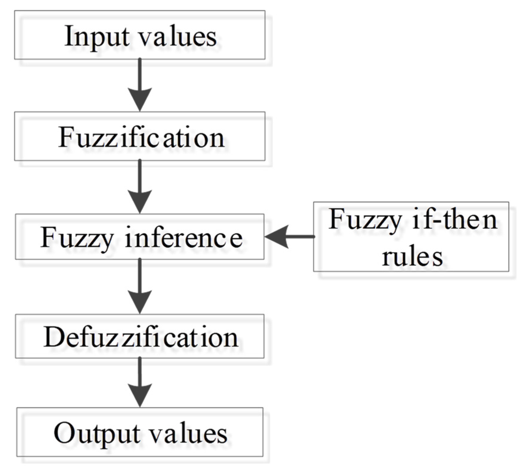
For convenience, the actual values of range, radial velocity and priority are normalized, as shown by the x axis in Figure 2. The normalized values are fuzzed with the triangular fuzzy number, which possesses a simple representation and strong anti-interference ability [34,35]. The membership functions, which are employed for the fuzzy values of the range and radial velocity, are presented for the evaluation of the priorities of the radars.

Based on the permutation and combination of the fuzzy values in Table 1, 49 if–then inferential rules are generated by intuitive and expert considerations. Then, we need to perform the fuzzy inference in accordance with the fuzzy rules. On account of the simple calculation steps and the accurate calculation results, the Larsen inference is utilized here [45]. Through the fuzzy inference, the fuzzy sets of the priority are obtained.

In order to use the priority in the actual calculation, we defuzzify the fuzzy sets of the priority to generate an exact value. The center average defuzzifier is adopted owing to the characteristics of plausibility, computational simplicity and continuity [46].

Through the aforementioned analysis, the FLIS can calculate the exact values of the priorities with the following process in Figure 3.

4.3. Optimization Modeling

According to Equation (31), it can be seen that the decision vectors of the target tracking error are the binary vector u_k and the power vector P_k. For the predetermined radar number M₁ and the tracking error η_k, we should select the optimal combination of the radars and allocate the power among these radars. The initial optimization model of the resource allocation is

$$\begin{array}{l}\min {\mathbf{1}}_M^{\mathrm{T}}{P}_k\\ s.t.\\ u_{m,k}\in \left\{0,1\right\}, m=1,2,\cdots ,M\\ \{\begin{array}{l}{P}_{m,k}>P_{\min }, u_{m,k}=1\\ P_{m,k}=0, u_{m,k}=0\end{array}\\ {\mathbf{1}}_M^{\mathrm{T}}{P}_k\le P_{\mathrm{total}} \\ F\left(u_k,P_k\right)\le {\eta }_k\end{array}$$

(32)

where $1_M^T$ = [1,1, …,1]_1×M.

In this model, the solving process of the binary vector u_k is dim, which makes the model inaccurate. We will make some modifications to this model in the upcoming step. Assume that the priority vector of all the radars is Pri_k = [pri_1,k, pri_2,k, …, pri_M,k]. We define the vector ${Pri}_k^{\mathrm{order}}$ and IN_k as

$$\left(Pr{i}_k^{\mathrm{order}},I{N}_k\right)=\mathrm{sort}\left(Pr{i}_k\right)$$

(33)

where sort(•) denotes the descending operator. ${\mathbf{P}\mathbf{r}\mathbf{i}}_k^{\mathrm{order}}$ is the descending order of Pri_k. IN_k indicates the positions of the elements in ${\mathbf{P}\mathbf{r}\mathbf{i}}_k^{\mathrm{order}}$ within Pri_k. Through the above derivation, the optimal combination $u_k^{M_1,\mathrm{opt}}$ of the selected radars is denoted as

$$u_k^{M_1,\mathrm{opt}}=\{\begin{array}{l}1, m=I{N}_k\left(1:M_1\right)\\ 0, \mathrm{others}\end{array}$$

(34)

For a specified $u_k^{M_1,\mathrm{opt}}$, the corresponding power allocation model is modified conditioned on Equation (32).

$$\begin{array}{l}\min {\mathbf{1}}_M^{\mathrm{T}}{P}_k^{M_1}\\ s.t.\\ \{\begin{array}{l}{P}_{m,k}\ge P_{\min }, u_{m,k}^{M_1,\mathrm{opt}}=1\\ P_{m,k}=0, u_{m,k}^{M_1,\mathrm{opt}}=0\end{array}\\ {\mathbf{1}}_M^{\mathrm{T}}{P}_k^{M_1}\le P_{\mathrm{total}} \\ F\left(u_k^{M_1,\mathrm{opt}},P_k^{M_1}\right)\le {\eta }_k\end{array}$$

(35)

where $P_k^{M_1}$ denotes the transmit power of the corresponding M₁ radar nodes.

The target RCS h_m,k is affected by the identification, attitude, position, aspect angle, wave length, polarization, etc. The target RCS h_m,k is unknown and uncertain, and we consider it as an uncertain variable with a random distribution [30]. However, the deterministic resource allocation model cannot handle the uncertainty and guarantee the robustness of the model. Let $h_k^{M_1}$ denote the corresponding RCS. The stochastic CCP is introduced to package the deterministic resource allocation model, which is reformulated as follows:

$$\begin{array}{l}\min {\mathbf{1}}_M^{\mathrm{T}}{P}_k^{M_1}\\ s.t.\\ \{\begin{array}{l}{P}_{m,k}\ge P_{\min }, u_{m,k}^{M_1,\mathrm{opt}}=1\\ P_{m,k}=0, u_{m,k}^{M_1,\mathrm{opt}}=0\end{array}\\ {\mathbf{1}}_M^{\mathrm{T}}{P}_k^{M_1}\le P_{\mathrm{total}}, \\ \mathrm{Pr}\left(F\left(u_k^{M_1,\mathrm{opt}},P_k^{M_1},h_k^{M_1}\right)\le {\eta }_k\right)\ge \delta \end{array}$$

(36)

where Pr(•) denotes the probability. δ denotes the confidence level.

4.4. Solution Strategy

The CCP makes sure that the stochastic constraints of the resource management hold at least with the confidence level δ. In this section, this uncertain programming is solved by the HIOA, which integrates the stochastic simulation and GA [31]. This algorithm is universal and can solve any uncertain programming models. The detailed process is shown as follows.

4.4.1. Stochastic Simulation

According to the expert experience and historical measurement data, assume that there exist N_k historical observations h_i,k (i = 1, 2, …, N_k) of RCS for all radar nodes. In practice, only M₁ radar nodes transmit beams to illuminate the target at each sampling instant, i.e., the RCS participating in calculation is denoted as $h_{i,k}^{M_1}$. Equivalently, we can generate N_k random variables $F\left(u_k^{M_1,\mathrm{opt}},P_k^{M_1},h_{i,k}^{M_1}\right)$ according to the historical RCS. The solving steps are illustrated as follows in

Table 2. The process of stochastic simulation.

Step 1 Let N′ = 0;

Step 2 Select $h_{i,k}^{M_1}$ (i = 1, 2, …, Nk) from the set and produce $F\left(u_k^{M_1,\mathrm{opt}},P_k^{M_1},h_{i,k}^{M_1}\right)$;

Step 3 If $F\left(u_k^{M_1,\mathrm{opt}},P_k^{M_1},h_{i,k}^{M_1}\right)$ ≤ ηk, N′ = N′ + 1;

Step 4 Repeat the second and third steps Nk times;

Step 5 $\mathrm{Pr}\left(F\left(u_k^{M_1,\mathrm{opt}},P_k^{M_1},h_{i,k}^{M_1}\right)\le {\eta }_k\right)$ = N′/Nk. If N′/Nk ≥ δ, the $u_k^{M_1,\mathrm{opt}}$ and $P_k^{M_1}$ meet the constraints, otherwise not.

[31].

4.4.2. Hybrid Intelligent Optimization Algorithm

Only one set of ($u_k^{M_1,\mathrm{opt}}$, $P_k^{M_1}$) is generated during each stochastic simulation. We need to execute the stochastic simulation many times to find the optimal ($u_k^{M_1,\mathrm{opt}}$, $P_k^{M_1,\mathrm{opt}}$), which can be efficiently obtained by the HIOA presented in

Table 3. The process of hybrid intelligent optimization algorithm.

(1) Initialize the population, and check the feasibility of the generated chromosomes by the stochastic simulation in Table 2.

(2) Update the chromosomes by crossover and mutation in which the feasibility of offspring can be checked by the stochastic simulation in Table 2.

(3) Calculate the objective function values of all the chromosomes.

(4) Compute the fitness of each chromosome according to the objective function values.

(5) Select the chromosomes by spinning the roulette wheel.

(6) Repeat the second to fifth steps for a given number of cycles.

(7) Report the best chromosome as the optimal solution $P_k^{M_1,\mathrm{opt}}$.

.

4.4.3. Closed-Loop Signal Processing Framework

In practice, according to the aforementioned modeling process, the joint resource allocation is decomposed into two steps. The first step is to select the radar nodes for illuminating the target, and the second step is to allocate the power among the selected radars. Of course, we can also not specify the number of working radars, and the power resource is allocated among all the radars. However, the working environment of radar systems varies. Hence, based on the demand pull of radar missions, the power resource is allocated among the radars of the specified number M₁.

In the resource allocation process, radar node selection and power allocation have a coupling relationship. The problem is whether the two-step solution strategy that we used can obtain the global optimal solution. The detailed analysis process is as follows.

After resource allocation, the centralized PC-FIM J(u_k, P_k) at instant k is calculated as Equation (29), and

$${\displaystyle \sum _{m=1}^M{u}_{m,k}}=M_1$$

(37)

where M₁ is the number of radars illuminating the target.

Clearly, since the PIM J_P(ξ_k|Z_k−1) is only related to the target motion equation, it will not be affected no matter which radar illuminates the target. Combining Equations (17) and (29), only the data information matrix (DIM) J_D(ξ_k|Z_k−1) is affected by the radar node selection and power allocation.

$$J_{\mathrm{D}}\left({\mathsf{\xi }}_k|Z_{k-1}\right)={\displaystyle \sum _{m=1}^M{u}_{m,k}{J}_{\mathrm{D}}\left(P_{m,k}\right)}$$

(38)

Assume that the transmit power of each radar is not zero, i.e., u_m,k = 1, and we collect J_D(ξ_k|Z_k−1) into a vector

$$J_{\mathrm{D}}=\left\{J_{\mathrm{D}}\left(P_{1,k}\right),J_{\mathrm{D}}\left(P_{2,k}\right),\cdots ,J_{\mathrm{D}}\left(P_{M,k}\right)\right\}$$

(39)

If the transmitting power of each radar is equal, the J_D(P_m,k) with longer distance has a smaller value. In addition, it can be seen from (25) and (27) that J_P(ξ_k|Z_k−1) and J_D(ξ_k|Z_k−1) are both positive definite matrixes. Since the PC-CRLB C_PC-CRLB(u_k, P_k) is the inverse matrix of J(u_k, P_k), the smaller J_D(P_m,k) with longer distance will obtain a greater C_PC-CRLB(u_k, P_k). In order to obtain a smaller target tracking error, the long-range radar will consume more power.

The fuzzy logic inference algorithm used in this paper calculates the priority of each radar according to the range and radial velocity, and the range plays a major role. The selected radars are those with closer ranges and those that consume less power. Based on this, the solution strategy of the adopted resource allocation model can also obtain the global optimal solution.

In the rest of this section, the closed-loop signal processing framework is summarized for the MTT in a centralized OAR network.

At first, the MCS-based ST-SCKF is utilized to fuse the received signal from each radar node through the CFC. In this fusion process, the global posterior estimate is computed by the sequential updating scheme, in which the most accurate local measurement should be updated first so as to reduce subsequent linearization errors. We adopt the FLIS to evaluate the priority of the target corresponding to different radar nodes by intelligent and valid means. As a more accurate bound to quantify the tracking performance, the centralized PC-CRLB is utilized as the optimization criterion for the selected radar nodes. The stochastic CCP of the resource allocation is solved by the HIOA. Thus, the joint resource allocation strategy realizes the optimal node and power allocation, which in turn benefits the target tracking. The integrated closed-loop feedback system is in

Table 4. The process of closed-loop signal processing.

(1) Let k = 1, initialize the ($u_k^{M_1,\mathrm{opt}}$, $P_k^{M_1,\mathrm{opt}}$).

(2) The MCS-based ST-SCKF with the sequential updating technique is used to obtain the global state estimate.

(3) Based on the updated target state, obtain the optimal radar nodes according to the priority.

(4) Compute the centralized PC-CRLB conditioned on a particle filter, and adopt the HIOA to solve the CCP-based resource allocation for the optimal solution.

(5) Send the optimal allocation ($u_{k+1}^{M_1,\mathrm{opt}}$, $P_{k+1}^{M_1,\mathrm{opt}}$) back to guide probing in next sampling instant.

(6) Let k = k + 1, and go to (2).

.

4.5. Further Statement

Statement 1: Three bounds are developed to quantify the MSE of the target state estimates in the published literature. The PCRLB is derived by taking the expectation with the joint distribution of ξ_k and Z_k up to the current time, i.e., it considers the measurements as random vectors and quantifies the target tracking performance conditioned on all the data possibly received [25]. However, the actually received measurements are the key in characterizing tracking performance in the upcoming moment. Accordingly, the conditional PCRLB is developed and conditioned on all the received data Z_1:k−1. Nevertheless, taking the average over all past measurement data weakens the tightness of the bound close to the MSE [26]. In practice, the tracking performance at time k has the closest connection with the measurement Z_k−1. Hence, the PC-CRLB, which is averaged over the joint density of ξ_k and Z_k conditioned on Z_k−1, is the tightest bound to the PC-MSE matrix in Equation (20). After comprehensive comparison, the PC-CRLB is the optimal alternative.

Statement 2: In the MCS-based ST_SCKF, the target state is updated according to the measurement from one node at a time, i.e., the sequential updating technique. Since the measurement model is nonlinear, we should update the target state with the measurement from the most accurate radar node to reduce subsequent linearization errors. Otherwise, the measurement errors will be amplified in the sequential procedure, even resulting in divergence.

5. Simulations and Analysis

In this section, we present some simulation results and analyses to demonstrate the effectiveness of the proposed resource allocation strategy. Here, we consider a centralized tracking scenario with eight radar nodes and a maneuvering target. The effective bandwidth and the effective time duration are set to B_m,k = 5 MHz and T_m,k = 1 ms, respectively. The carrier frequency of each transmitting signal is set to 10 GHz and the carrier wavelength is λ_m = 0.03 m. The number of the coherent pulses is 64. The lower bound of the transmitting power is P_min = 0.1 P_total. A sequence of 40 frames with the sampling interval T₀ = 1 s is adopted for the simulation process. The initial maneuvering frequency is α = 0.1, and the initial forgetting factor is ρ_f = 0.95. Without loss of generality, assume that the target reflectivity h_m,k has the same distribution function, which is modeled as a Swerling I model with the mean being 0.3. The initial states of the radars and the target are shown in

Table 5. The initial target state and the radar coordinates.

Index	Initial Position (km)	Velocity (m/s)
Radar 1	(18, 0)	(-, -)
Radar 2	(25, 0)	(-, -)
Radar 3	(35, 5)	(-, -)
Radar 4	(45, 10)	(-, -)
Radar 5	(15, 20)	(-, -)
Radar 6	(25, 24)	(-, -)
Radar 7	(35, 24)	(-, -)
Radar 8	(45, 24)	(-, -)
Case 1: Target	(20, 9)	(380, 440)
Case 2: Target	(46, 16)	(−600, −250)

. The display and analysis of subsequent simulations are divided into two cases.

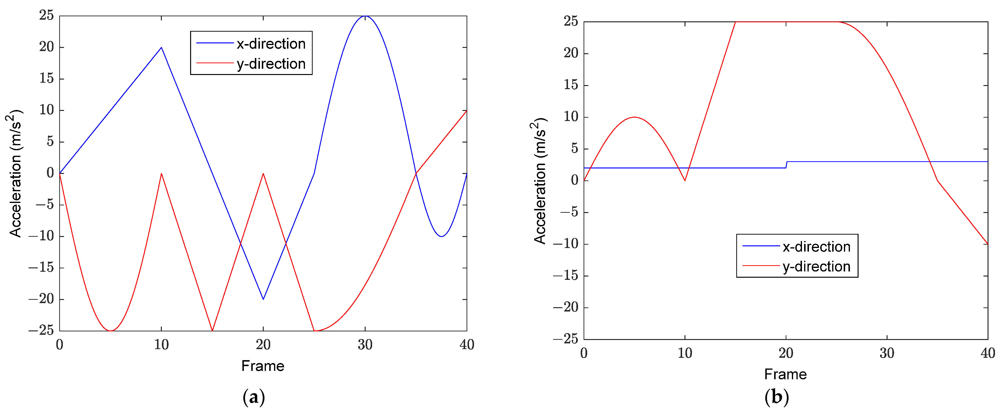
In Case 1, the target has great maneuverability in both the x and y directions, and we let three radars track the target through the whole tracking process. The target tracking is shown by the blue line in Figure 4, and the acceleration model is shown in Figure 5a.

In Case 2, only the acceleration in the y direction changes greatly over time, and we let four radars track the target. The target tracking is shown by the red line in Figure 4, and the acceleration model is shown in Figure 5b.

Just to be clear, except for the comparison of resource consumption at different confidence levels, without restricting generality, the confidence levels are all set to δ = 0.9 in other simulations of the following two cases.

5.1. Case 1: 3 Radars and Acceleration Model 1

5.1.1. Adaptive Priority

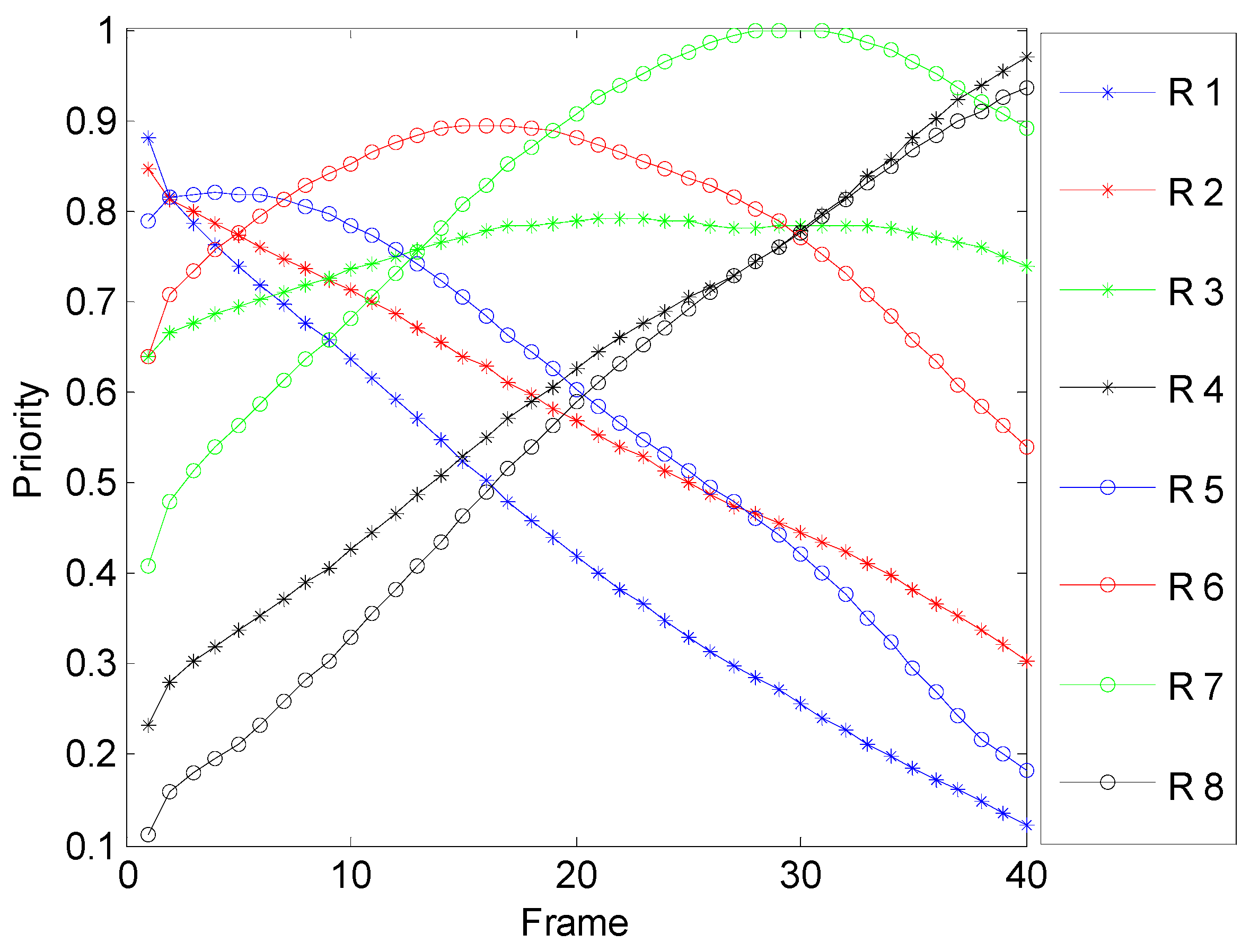
The priority of the radars at each sampling interval is updated in real time according to the range and the radial velocity. Although two influencing factors are considered for the priority, the relative range between the target and the radars plays a decisive role. Figure 6 depicts the radar priority which varies with the target state. Together with Figure 4, we can obviously identify that the three nearest radars, i.e., radar 1, 2 and 5, have the highest priority in the initial period. As time goes on, the three selected radars become radar 3, 6 and 7. Finally, radar 4, 7 and 8 have the highest priority. Throughout the tracking process, the range dominates the priority with the reason being that the received signal strength is inversely proportional to the quadratic power of the range, as shown in Equation (4).

Figure 7 gives the radar serial number in the working state at each frame. Through comparison with Figure 6, we find that the working radars are the three radars with the highest priority.

5.1.2. Power Allocation with Different Conditions

We then proceed with our simulations to compare the power consumption under different conditions. Figure 8 presents the optimal power allocation results at each sampling instant with the same confidence. They are all normalized with the total transmitting power of each frame. The radar with the largest power consumption changes continually with the movement of the target.

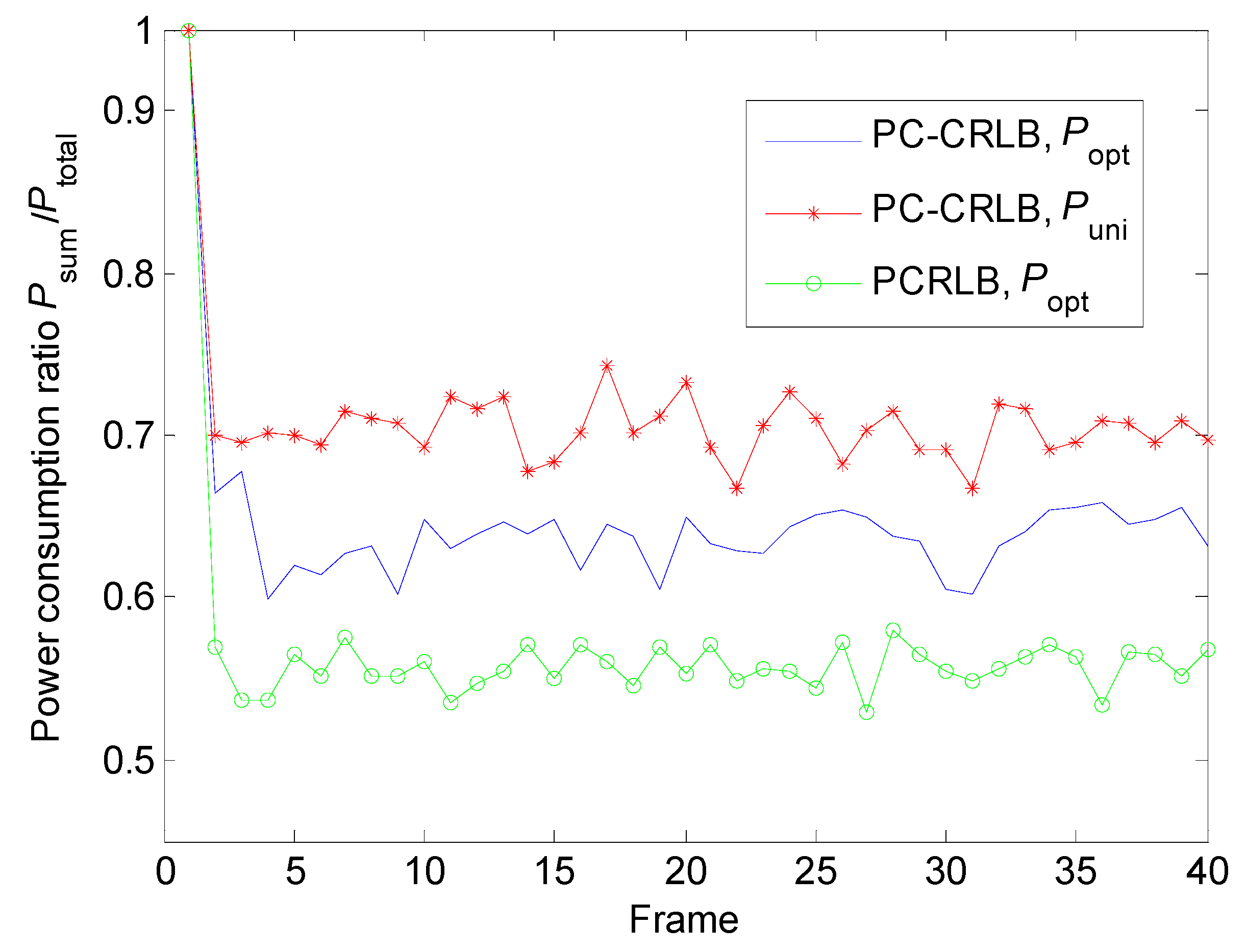
In Figure 9, P_sum denotes the sum of transmitting power of all radars, and P_total denotes the rated power of the OAR system. This figure describes the total power consumption with respect to different power allocation algorithms and different tracking performance criteria. Here, we need to explain the three curves in detail. While the PC-CRLB is adopted as the optimization criterion, as shown by the blue curve and the red curve in Figure 9, the adaptive allocation algorithm could reduce the power consumption by 18% compared to the uniform allocation algorithm. In addition, through comparing the optimal power allocation with different optimization criterions, as shown by the blue curve and the green curve, we find that the total power consumption based on PC-CRLB is more than the counterpart based on PCRLB. The reason is as follows: The PC-CRLB provides a tighter lower bound on the MSE of any estimator than the PCRLB, i.e., the PC-CRLB is larger than the PCRLB with respect to a specific estimate. For a preset tracking error threshold, the allocation algorithm with the PC-CRLB has to consume more power. The comparison of the total power consumption between PC-CRLB and PCRLB demonstrates from the reverse side that PC-CRLB is a more accurate bound.

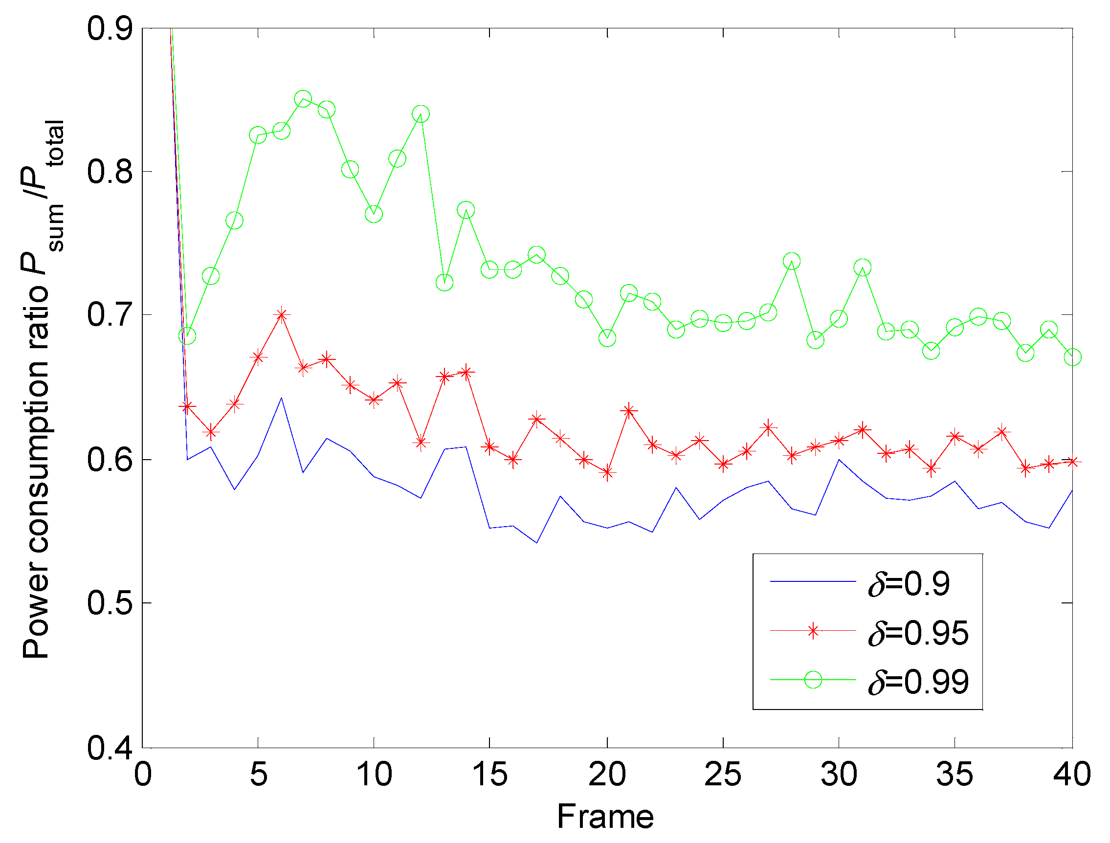
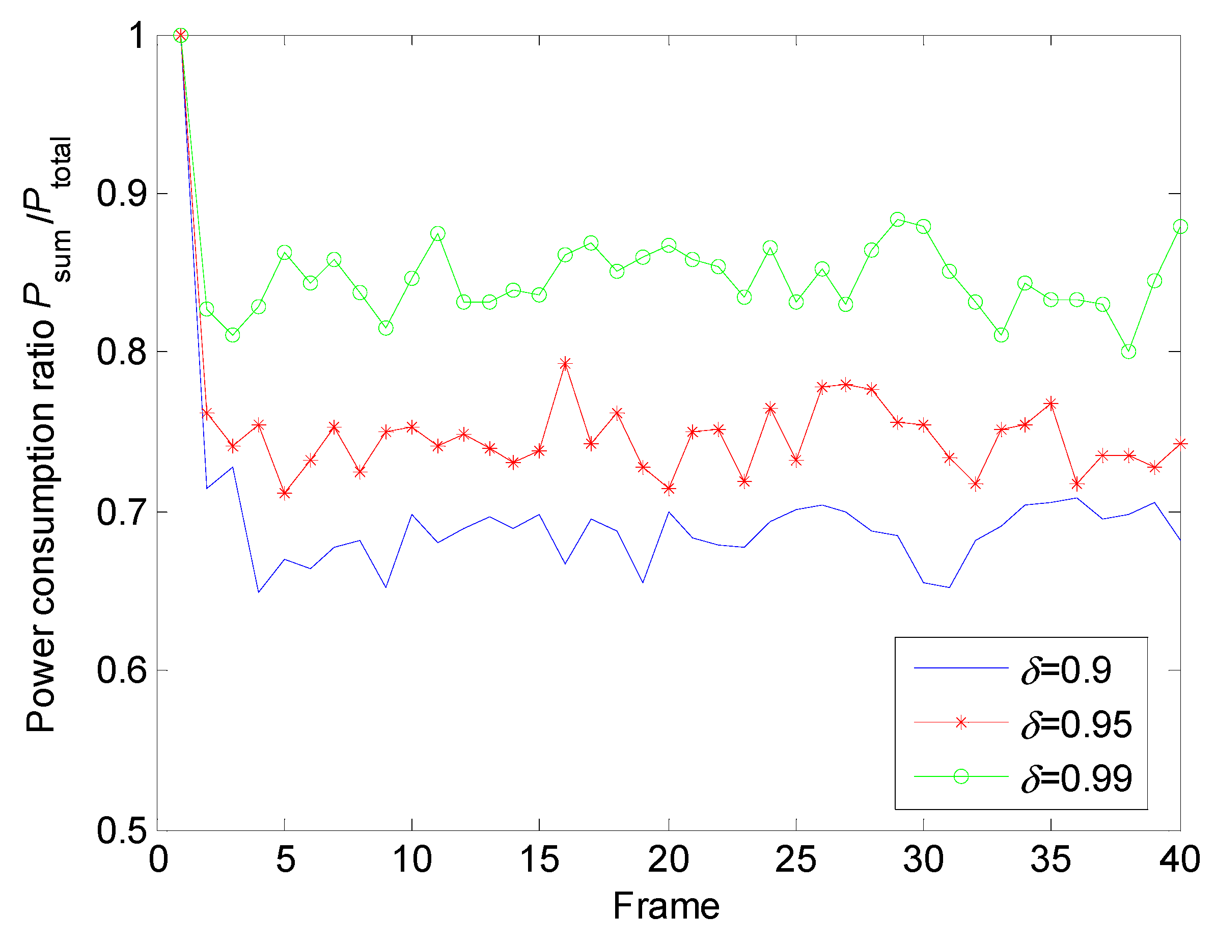
The total power consumption is relative to the confidence level. In general, the appropriate confidence levels are selected in accordance with tracking scenarios. Herein, we specify the confidence level δ as 0.99, 0.95 and 0.9 in Figure 10. The requirement for power decreases as the reliability of the inequality decreases. Hence, it is clear that the power consumption is proportional to the confidence levels.

5.1.3. Target Tracking

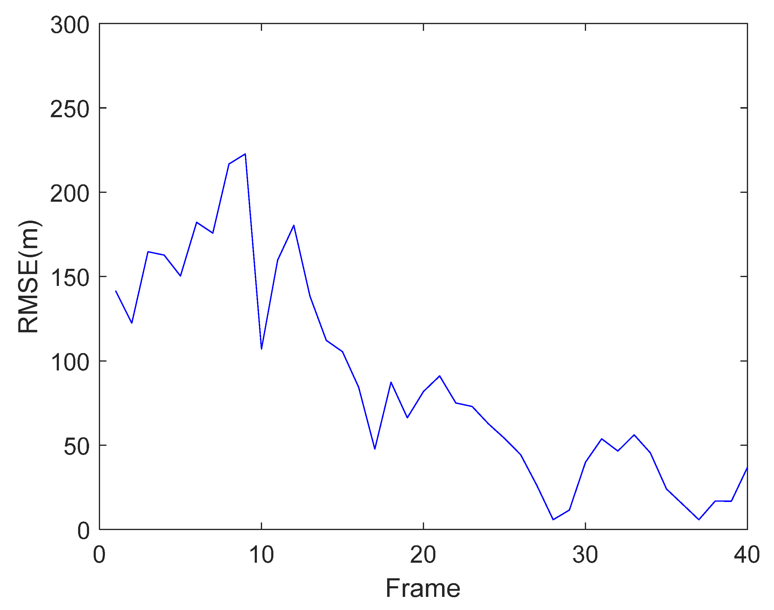
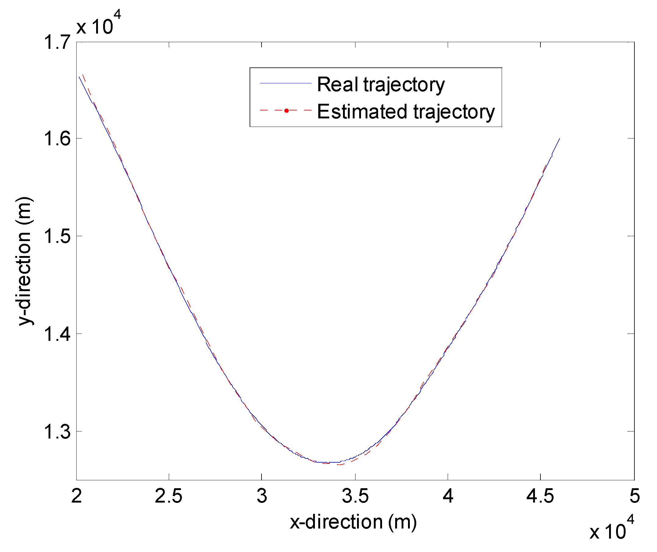
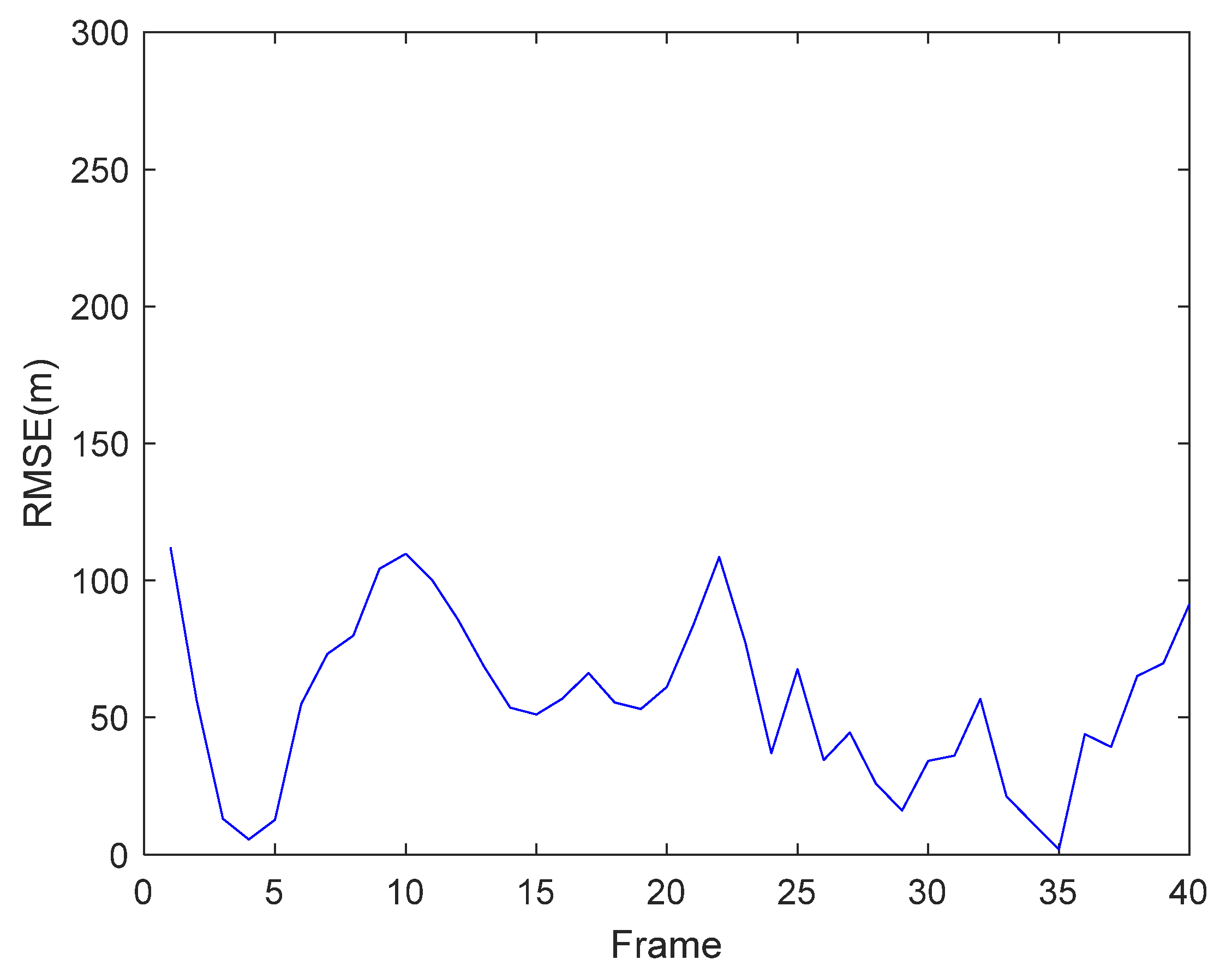
Figure 11 shows the estimated trajectory and the actual trajectory of the target. Combined with Figure 4, although the maneuverability of the target is very high in the x and y directions in the whole tracking process, the tracking effect is satisfactory. Figure 12 gives the root MSE (RMSE) of the target.

In the simulation, the stochastic simulation is embedded into the GA to form an HIOA to solve CCP problems. The two sub-algorithms are quite time-consuming. It takes 513 s to solve the model in Case 1.

5.2. Case 2: Four Radars and Acceleration Model 2

5.2.1. Adaptive Priority

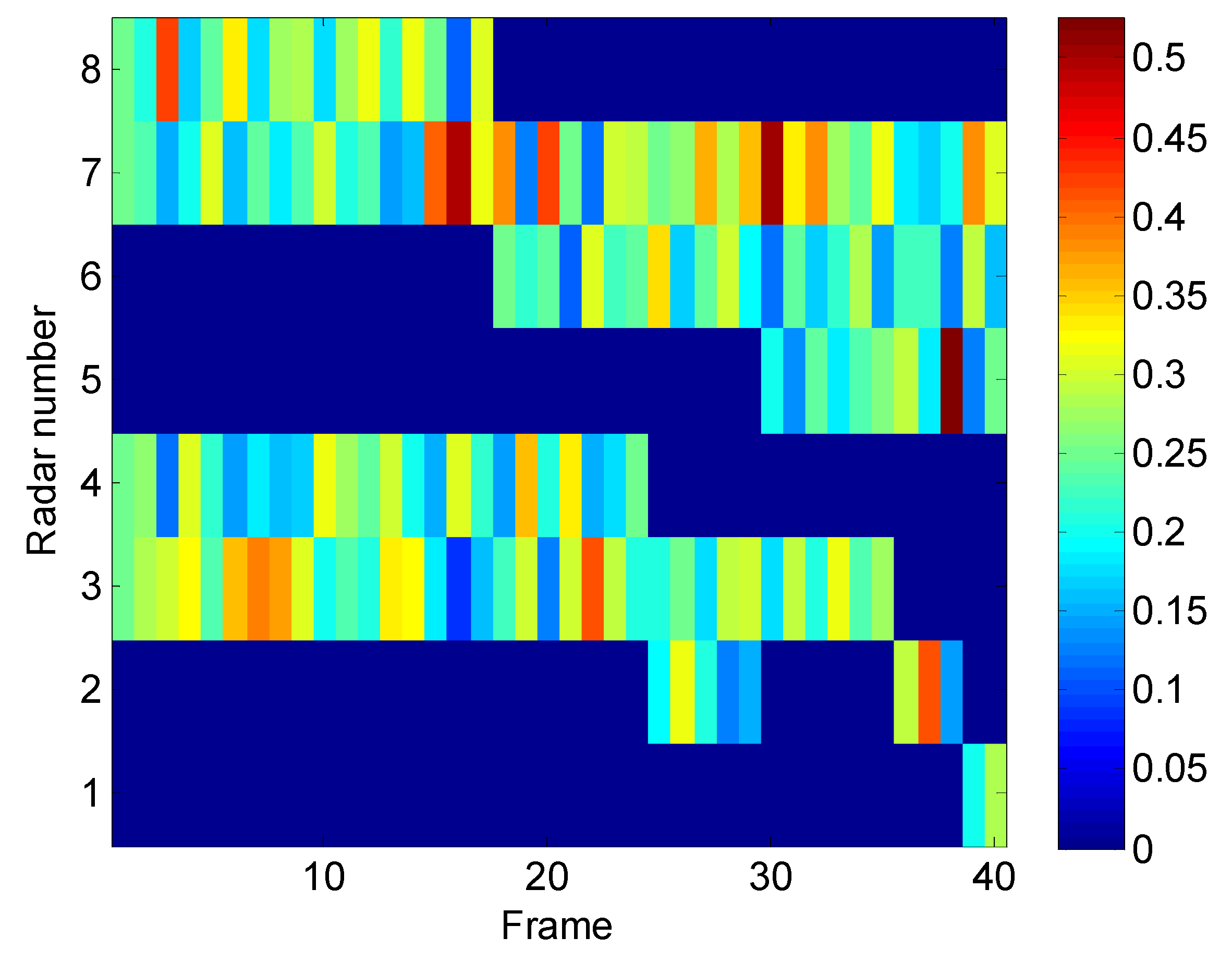
The priority of the radars is still updated in line with the range and the radial velocity. Since the starting position and moving track of the target are different from the situation in Case 1, the radars close to the starting point have higher priority at the beginning, such as radars 3, 4, 7 and 8. Other radars also occupy the high-priority positions for a short time as the target moves. In addition, the high acceleration in the y direction shown in Figure 5b makes the target turn to the positive direction of the y coordinate. Radar 7 has high priority through the whole tracking process. Combining Figure 13 and Figure 14, we can obtain a clearer conclusion.

5.2.2. Power Allocation with Different Conditions

Figure 15 depicts the optimal power allocation with four radars. Compared with Figure 8, we add a new radar to the radar working group. The newly added radar has lower priority than the other three radars. Under the condition that the target tracking performance remains unchanged, the addition of a new radar will reduce the transmitting power of other radars in the tracking process. Hence, we find that the red boxes are reduced in Figure 15. Simultaneously, the lower priority makes the transmitting power of this radar larger than the sum of the power reductions in other radars. Based on this, the total transmitting power in Figure 16 is higher than its counterpart in Figure 9 conditioned on the same tracking performance.

The total power consumption is shown in Figure 16 with the same confidence level. Under the same desired tracking error, the size relationships of power consumption among the three conditions are similar to the relationships in Figure 9. The distinction between the two figures is that the total power consumption in Figure 16 is larger than the counterpart in Figure 9, which is attributed to the increase in radars. For a detailed explanation for Figure 16, one could refer to the analysis of Figure 9.

Figure 17 describes the total power consumption conditioned on different confidence levels. The variation of Figure 17 with respect to Figure 10 is similar to the variation of Figure 16 with respect to Figure 9.

5.2.3. Target Track

Figure 18 and Figure 19 show effective target tracking. These figures demonstrate that we realize the optimal resource allocation without losing tracking performance. It consumes more time to allocate system resources among more radar nodes, and it takes 625 s to solve the model in Case 2.

6. Conclusions and Future Work

In this paper, we develop a robust resource allocation strategy for MTT in a netted OAR system under uncertain conditions. First, we obtain the global posterior estimate of the target state conditioned on the optimal fusion through a closed-loop signal processing framework. The FLIS infers the optimal tracking radars according to the relative motion states of the target. Due to the large measurement error caused by the high maneuverability of the target, we deduce the centralized PC-CRLB as the optimization criterion to bound the target state estimate error. Finally, the resource allocation model encapsulated with the CCP is solved by an HIOA, and the power allocation results are sent back to guide the resource allocation for the upcoming probing period. Simulation results show that the resource allocation strategy can effectively improve the overall power utilization rate. The derived PC-CRLB provides a tighter bound than the PCRLB. The CCP model enables the robust power allocation conditioned on different confidence levels.

In this paper, the stochastic simulation is embedded into the GA to form the HIOA. Stochastic simulation uses the Monte Carlo method to generate random variables according to probability distribution, and it takes a lot of time. Moreover, as a kind of intelligent optimization algorithm, a GA has a slow computational speed and is prone to converging prematurely. Motivated by the aforementioned problems, finding a fast algorithm for solving uncertain programming is an urgent problem to be solved. This is also the direction we need to work in in the future. On the other hand, the sharp increase in commercial wireless communications services has resulted in the problem of radio frequency electromagnetic spectrum congestion. Driven by the need to improve spectrum exploitation, the joint optimization of power resources and spectrum resources, or resource optimization under the condition of integrated radar and communication systems, is also worth studying.

References

1. Kocaman, İ. Distributed Beamforming in a Swarm UAV Network. Master’s Thesis, Naval Postgraduate School, Monterey, CA, USA, 2008. [Google Scholar]
2. Long, W.J.; Ben, D.; Pan, M.H.; Shu, X.R.; Han, Y.M.; Pan, J.B. Opportunistic digital array radar and its technical characteristic analysis. In Proceedings of the IET International Radar Conference, Guilin, China, 20–22 April 2009. [Google Scholar]
3. Han, Q.H.; Pan, M.H.; Liang, Z.L. Joint power and beam allocation of opportunistic array radar for multiple target tracking in clutter. Digit. Signal Process. 2018, 78, 136–151. [Google Scholar] [CrossRef]
4. Han, Q.H.; Pan, M.H.; Long, W.J.; Liang, Z.L.; Shan, C.G. Joint adaptive sampling interval and power allocation for maneuvering target tracking in a multiple opportunistic array radar system. Sensors 2020, 20, 981. [Google Scholar] [CrossRef] [PubMed]
5. Zeng, J. Evolution of netted radar systems. IEEE Access 2020, 8, 124961–124977. [Google Scholar]
6. Yan, J.K.; Liu, H.W.; Jiu, B.; Chen, B.; Liu, Z.; Bao, Z. Simultaneous multibeam resource allocation scheme for multiple target tracking. IEEE Trans. Signal Process. 2015, 63, 3110–3122. [Google Scholar] [CrossRef]
7. Yuan, Y.; Yi, W.; Hoseinnezhad, R.; Varshney, P.K. Robust power allocation for resource-aware multi-target tracking with colocated MIMO radars. IEEE Trans. Signal Process. 2021, 9, 443–458. [Google Scholar] [CrossRef]
8. Lu, X.J.; Yi, W.; Kong, L.J. Joint online route planning and resource optimization for multitarget tracking in airborne radar systems. IEEE Syst. J. 2022, 16, 4198–4209. [Google Scholar] [CrossRef]
9. Yang, Y.Q.; Xia, Z.H.; Zhao, Z.L.; Zhang, T.; Li, K.; Yin, X.; Shi, H.F.; Peng, T. Intelligent resource management and optimization of clustered UAV airborne SAR system. In Proceedings of the 2021 IEEE 4th International Conference on Electronics Technology (ICET), Chengdu, China, 7–10 May 2021. [Google Scholar]
10. Godrich, H.; Petropulu, A.P.; Poor, H.V. Power allocation strategies for target localization in distributed multiple-radar architectures. IEEE Trans. Signal Process. 2011, 59, 3226–3240. [Google Scholar] [CrossRef]
11. Godrich, H.; Petropulu, A.P.; Poor, H.V. Sensor selection in distributed multiple-radar architectures for localization: A knapsack problem formulation. IEEE Trans. Signal Process. 2012, 60, 247–260. [Google Scholar] [CrossRef]
12. Yan, J.K.; Pu, W.Q.; Liu, H.W.; Jiu, B.; Bao, Z. Robust chance constrained power allocation scheme for multiple target localization in colocated MIMO radar system. IEEE Trans. Signal Process. 2018, 66, 3946–3957. [Google Scholar] [CrossRef]
13. Xie, M.C.; Yi, W.; Kirubarajan, T.; Kong, L.J. Joint node selection and power allocation strategy for multitarget tracking in decentralized radar networks. IEEE Trans. Signal Process. 2018, 66, 729–743. [Google Scholar] [CrossRef]
14. Yan, J.K.; Pu, W.Q.; Zhou, S.H.; Liu, H.W.; Greco, M.S. Optimal resource allocation for asynchronous multiple targets tracking in heterogeneous radar networks. IEEE Trans. Signal Process. 2020, 68, 4055–4068. [Google Scholar] [CrossRef]
15. Sun, H.; Li, M.; Zuo, L.; Cao, R.Q. Joint threshold optimization and power allocation of cognitive radar network for target tracking in clutter. Signal Process. 2020, 172, 107566. [Google Scholar] [CrossRef]
16. Zhang, H.W.; Liu, W.J.; Zhang, Z.J.; Lu, W.L.; Xie, J.W. Joint target assignment and power allocation in multiple distributed MIMO radar networks. IEEE Syst. J. 2021, 15, 694–704. [Google Scholar] [CrossRef]
17. Zhang, R.S.; Zhang, J.Y.; Yu, H.C. Review of modeling and control in UAV autonomous maneuvering flight. In Proceedings of the 2018 IEEE International Conference on Mechatronics and Automation (ICMA), Changchun, China, 5–8 August 2018. [Google Scholar]
18. Dong, F.; You, K.Y.; Zhang, J.Q. Flight control for UAV loitering over a ground target with unknown maneuver. IEEE Trans. Control Syst. Tech. 2020, 28, 2461–2473. [Google Scholar] [CrossRef]
19. Guo, L.; Li, X.R.; Huang, H.; Jing, S.; He, Y.C.; Wang, C.Z. Intelligent penetration of UAV based on moth suppression algorithm. In Proceedings of the 2018 Chinese Automation Congress (CAC), Xi’an, China, 30 November–2 December 2018. [Google Scholar]
20. Liang, L.; Deng, F.; Wang, J.N.; Lu, M.B.; Chen, J. A reconnaissance penetration game with territorial-constrained defender. IEEE Trans. Autom. Control 2022, 67, 6295–6302. [Google Scholar] [CrossRef]
21. Nadarajah, N.; Tharmarasa, R.; McDonald, M.; Kirubarajan, T. IMM forward filtering and backward smoothing for maneuvering target tracking. IEEE Trans. Aerosp. Electron. Syst. 2012, 48, 2673–2678. [Google Scholar] [CrossRef]
22. Ma, J.; Guo, X.T. Combination of IMM algorithm and ASTRWCKF for maneuvering target tracking. IEEE Access 2020, 8, 143095–143103. [Google Scholar] [CrossRef]
23. Zhang, Z.H.; Zhou, G.J. Maneuvering target state estimation based on separate modeling with high-order polynomials. Digit. Signal Process. 2022, 123, 103401. [Google Scholar] [CrossRef]
24. Savage, C.O.; La Scala, B.F. Sensor management for tracking smart targets. Digit. Signal Process. 2009, 19, 968–977. [Google Scholar] [CrossRef]
25. Zuo, L.R.; Niu, X.; Varshney, P.K. Conditional Posterior Cramér-Rao Lower Bounds for Nonlinear Sequential Bayesian Estimation. IEEE Trans. Signal Process. 2011, 59, 1–14. [Google Scholar] [CrossRef]
26. Bell, K.L.; Baker, C.J.; Smith, G.E.; Johnson, J.T.; Rangaswamy, M. Cognitive radar framework for target detection and tracking. IEEE J. Sel. Topics Signal Process. 2015, 9, 1427–1439. [Google Scholar] [CrossRef]
27. Chen, X.; Tharmarasa, R.; Kirubarajan, T. Multitarget multisensor tracking. In Academic Press Library in Signal Processing; Sidiropoulos, N.D., Gini, F., Chellappa, R., Theodoridis, S., Eds.; Academic Press: Cambridge, MA, USA, 2014; Volume 2, pp. 786–787. [Google Scholar]
28. Li, X.T.; Zhang, T.X.; Yi, W.; Kong, L.J.; Yang, X.B. Radar selection based on the measurement information and the measurement compensation for target tracking in radar network. IEEE Sens. J. 2019, 19, 7923–7935. [Google Scholar] [CrossRef]
29. Zhang, H.W.; Liu, W.J.; Zhang, Q.; Fei, T.Y. A robust joint frequency spectrum and power allocation strategy in a coexisting radar and communication system. Chin. J. Aeronaut. 2024. [Google Scholar] [CrossRef]
30. Skolnik, M.I. Introduction to Radar System, 3rd ed.; Tata McGraw-Hill Publishing Company Limited: New Delhi, India, 2001; pp. 49–73. [Google Scholar]
31. Liu, B.D. Theory and Practice of Uncertain Programming, 2nd ed.; Springer: Berlin, Germany, 2009. [Google Scholar]
32. Zhang, H.W.; Liu, W.J.; Zong, B.F.; Shi, J.P.; Xie, J.W. An efficient power allocation strategy for maneuvering target tracking in cognitive MIMO radar. IEEE Trans. Signal Process. 2021, 69, 1591–1602. [Google Scholar] [CrossRef]
33. Zhang, H.W.; Xie, J.W.; Ge, J.A.; Lu, W.L.; Liu, B.Z. Strong tracking SCKF based on adaptive CS model for manoeuvring aircraft tracking. IET Radar Sonar Navig. 2018, 12, 742–749. [Google Scholar] [CrossRef]
34. Miranda, S.L.C.; Baker, C.J.; Woodbridge, K.; Griffiths, H.D. Knowledge-based resource management for multifunction radar. IEEE Signal Process. Mag. 2006, 23, 66–76. [Google Scholar] [CrossRef]
35. Miranda, S.L.C.; Baker, C.J.; Woodbridge, K.; Griffiths, H.D. Fuzzy logic approach for prioritisation of radar tasks and sectors of surveillance in multifunction radar. IET Radar Sonar Nav. 2007, 1, 131–141. [Google Scholar] [CrossRef]
36. Van Trees, H.L. Detection, Estimation, Modulation Theory Part III; Wiley: New York, NY, USA, 1971. [Google Scholar]
37. Singer, R.A. Estimating optimal tracking filter performance for manned maneuvering targets. IEEE Trans. Aerosp. Electron. Syst. 1970, AES-6, 473–483. [Google Scholar] [CrossRef]
38. Zhou, H.; Kumar, K.S.P. A ‘current’ statistical model and adaptive algorithm for estimating maneuvering targets. AIAA J. Guid. 1984, 7, 596–602. [Google Scholar] [CrossRef]
39. Mehrotra, K.; Mahapatra, P.R. A Jerk model for tracking highly maneuvering targets. IEEE Trans. Aerosp. Electron. Syst. 1997, 3, 1094–1105. [Google Scholar] [CrossRef]
40. Zhang, H.W.; Liu, W.; Shi, J.P.; Fei, T.; Zong, B. Joint detection threshold optimization and illumination time allocation strategy for cognitive tracking in a networked radar system. IEEE Trans. Signal Process. 2022, 70, 5833–5847. [Google Scholar] [CrossRef]
41. Van Trees, H.L. Optimum Array Processing: Detection, Estimation, Modulation Theory IV; Wiley: New York, NY, USA, 2001. [Google Scholar]
42. Van Trees, H.L.; Bell, K.L. Bayesian Bounds for Parameter Estimation and Nonlinear Filtering/Tracking; Wiley: New York, NY, USA, 2007. [Google Scholar]
43. Glass, J.D.; Smith, L.D. MIMO radar resource allocation using posterior Cramér-Rao lower bounds. In Proceedings of the 2011 IEEE Aerospace Conference, Big Sky, MT, USA, 5–12 March 2011; pp. 1–9. [Google Scholar]
44. Han, Q.H.; Pan, M.H.; Zhang, W.C.; Liang, Z.H. Time resource management of OAR based on fuzzy logic priority for multiple target tracking. J. Syst. Eng. Electron. 2018, 29, 742–755. [Google Scholar]
45. Lee, C.C. Fuzzy logic in control systems: Fuzzy logic controller, parts I and II. IEEE Trans. Syst. Man Cybern. 1990, 20, 404–435. [Google Scholar] [CrossRef]
46. Wang, L.X. A Course in Fuzzy Systems and Control (International Edition); Prentice-Hall: Upper Saddle River, NJ, USA, 1997. [Google Scholar]
Figure 1. The closed-loop signal processing framework, where i1, i2, …, is ∈ {1, 2, …, M}, and sM.
Remotesensing 16 03499 g001
Figure 2. Membership function of fuzzy variables. (a) Normalized range; (b) normalized radial velocity; (c) normalized priority.
Remotesensing 16 03499 g002
Figure 3. Integrated fuzzy logic inference system.
Remotesensing 16 03499 g003
Figure 4. The positional relationship of the radars and the target.
Remotesensing 16 03499 g004
Figure 5. Two maneuvering models of the target. (a) Case 1: acceleration model 1; (b) Case 2: acceleration model 2.
Remotesensing 16 03499 g005
Figure 6. Priority of radars over time in Case 1.
Remotesensing 16 03499 g006
Figure 7. Working radars in each frame in Case 1.
Remotesensing 16 03499 g007
Figure 8. Optimal power allocation of radars in Case 1.
Remotesensing 16 03499 g008
Figure 9. Total power consumption ratio under different conditions in Case 1.
Remotesensing 16 03499 g009
Figure 10. Total power consumption ratio under different conditions in Case 1.
Remotesensing 16 03499 g010
Figure 11. Target tracking in Case 1.
Remotesensing 16 03499 g011
Figure 12. RMSE of the target in Case 1.
Remotesensing 16 03499 g012
Figure 13. Priority of radars over time in Case 2.
Remotesensing 16 03499 g013
Figure 14. Working radars in each frame in Case 2.
Remotesensing 16 03499 g014
Figure 15. Optimal power allocation of radars in Case 2.
Remotesensing 16 03499 g015
Figure 16. Total power consumption ratio under different conditions in Case 2.
Remotesensing 16 03499 g016
Figure 17. Total power consumption ratio of different confidence levels in Case 2.
Remotesensing 16 03499 g017
Figure 18. Target tracking in Case 2.
Remotesensing 16 03499 g018
Figure 19. RMSE of the target in Case 2.
Remotesensing 16 03499 g019