Abstract
Accurate understanding of urban land use change information is of great significance for urban planning, urban monitoring, and disaster assessment. The use of Very-High-Resolution (VHR) remote sensing images for change detection on urban land features has gradually become mainstream. However, most existing transfer learning-based change detection models compute multiple deep image features, leading to feature redundancy. Therefore, we propose a Transfer Learning Change Detection Model Based on Change Feature Selection (TL-FS). The proposed method involves using a pretrained transfer learning model framework to compute deep features from multitemporal remote sensing images. A change feature selection algorithm is then designed to filter relevant change information. Subsequently, these change features are combined into a vector. The Change Vector Analysis (CVA) is employed to calculate the magnitude of change in the vector. Finally, the Fuzzy C-Means (FCM) classification is utilized to obtain binary change detection results. In this study, we selected four VHR optical image datasets from Beijing-2 for the experiment. Compared with the Change Vector Analysis and Spectral Gradient Difference, the TL-FS method had maximum increases of 26.41% in the F1-score, 38.04% in precision, 29.88% in recall, and 26.15% in the overall accuracy. The results of the ablation experiments also indicate that TL-FS could provide clearer texture and shape detections for dual-temporal VHR image changes. It can effectively detect complex features in urban scenes.
1. Introduction
Remote sensing image change detection is the process of detecting changes in the Earth’s surface using images of multiple time phases and comparative analysis to obtain information about changes in features [1]. In recent years, with the continuous progress in remote sensing satellites, people have continuously upgraded the resolution of remote sensing images and widely used very-high-resolution sensing images in urban environmental monitoring, meteorological monitoring, urban functional area planning, natural disaster monitoring, and changes in land surface coverage [2,3,4,5].
Compared with simple features such as with farmland, the features in urban areas are more complex, and Very-High-Resolution (VHR) remote sensing imagery can effectively show these complex features, so how to utilize these detailed features for change detection is extremely important [6]. For a single time-phase VHR image, various feature characteristics in urban areas are clearly expressed, and urban area features can be extracted by increasing the complexity and computation of the model [7]. However, there are some problems here; there are three drawbacks when computing a large number of image features if we use multitemporal images for change detection. Firstly, learning multiple features can lead to feature redundancy in the model [8]. Redundant features often do not contribute significantly to the model and can consume excessive resources [9]. Secondly, when conducting multitemporal remote sensing change detection, computing multiple urban surface features can introduce a large amount of irrelevant change features, which can negatively impact the detection effectiveness and, in some cases, even lead to adverse effects. Thirdly, for multitemporal remote sensing change detection, many feature objects are irrelevant to the changes. These irrelevant features can have side effects in certain aspects [10]. When processing a large number of features in image computation, there is an in-depth interpretation of image information. Although multitemporal images may have a positive effect within a certain range of feature values, an excess of similar features can affect the change detection results. The specific manifestations of these impacts are as follows: Firstly, for complex urban scenes in VHR images, feature redundancy can have negative effects [11]. For example, unclear and irregular textures of certain buildings and overly coarse edge detection can occur. Secondly, an excessive number of irrelevant change features can result in significant false positives and false negatives for impervious surfaces and vegetation, respectively. This prevents adaptive extraction of urban change information [12]. Therefore, it is necessary to design an algorithm for selecting change features to reduce the computational load while enhancing model performance.
We can broadly categorize image change detection methods into the following two main types: unsupervised and supervised [13]. Among these, unsupervised methods are more popular as they do not require training samples for detecting changes in land features. Traditional unsupervised methods include Change Vector Analysis (CVA) [14], Stochastic Gradient Descent (SGD) [15], Principal Component Analysis (PCA) [16], Iteratively Reweighted Multivariate Alteration Detection (IRMAD) [17], and Change Vector Analysis in Posterior Probability Space (CVAPS) [18], among others. These methods perform well on medium- to low-resolution remote sensing images. However, when applied to VHR images in urban areas, their performance tends to be weak. This is because these methods only utilize basic image features (such as spectral and texture features) to represent the images and cannot extract advanced features to represent changes in urban areas [19].
Currently, with the continuous iterations of computer hardware and software updates, using deep learning methods for change detection is an excellent choice. Deep learning has shown remarkable performance in remote sensing object detection, semantic segmentation, and other tasks [20]. Change detection commonly uses Convolutional Neural Networks (CNNs). Popular CNN models include U-Net [21], DeepLabV3 [22], GoogLeNet [23], LeNet-5 [24], AlexNet [25], ResNet [26], and various extensions. Researchers have used these networks in change detection tasks and have demonstrated excellent detection performance. However, utilizing CNNs for change detection also requires a large number of training samples. In practice, because of the complexity of urban environments, including factors such as dense buildings, traffic congestion, and crowded areas, it is challenging to obtain samples from complex urban areas, especially pixel-level training samples [27]. This necessitates high-resolution image data and fine pixel-level annotations, which incur significant human and time costs. Manual annotation for complex urban VHR images, including intricate urban structures, dense building layouts, and variable terrain features, is impractical. Therefore, Transfer Learning (TL) has gradually gained attention. It can achieve good results without the need for any training samples [28]. Researchers have proposed a series of methods for change detection tasks. The SENECA network can achieve good training results with only a small number of samples, but the model is complex and time-consuming [29]. The sample generation method based on transfer learning and superpixel segmentation, used for unsupervised change detection, produces good samples. However, it cannot adaptively select change features for dual-temporal changes [30]. Although the TCD-Net model has a low number of parameters and is sensitive to various land features, it lacks sensitivity to change information [31]. The transfer learning change detection model with 3D filters can extract multiple image features, but these features cannot be generalized, leading to redundant irrelevant change features [32]. Building upon this, researchers have proposed a method that combines advanced features with semantic change detection. This approach can compute the distance between various change vectors and generate better difference images. However, the method still fails to establish a relationship between changes and the model [28].
In the features extracted by transfer learning, it is difficult to establish a relationship between changes and the model. Some irrelevant changes in features can lead to redundancy, resulting in incomplete detection of changes in certain buildings and missed detections of vegetation in complex urban areas. Based on the analysis above, most change detection CNN models not only require a large amount of sample data for training but also demand sample accuracy at the pixel level [33]. Using pretrained models for transfer learning may indeed be a good choice. However, most pretrained models have a large number of parameters when extracting deep features, leading to redundant irrelevant change features. This inability to adaptively extract relevant change information can, in turn, impact the results of change detection. So some of the extracted features are change related features and some of the features are not change related. Therefore, we propose a change detection method, named TL-FS (Transfer Learning with Feature Selection), to address the issue of feature redundancy. As a classic CNN model structure, this paper utilizes the VGG16 model [34]. Firstly, we employ the pretrained VGG16 model to learn various features in the image scenes. Secondly, we use a change feature selection algorithm based on filter feature methods to filter change features [35,36]. Thirdly, all selected change features are combined into a multidimensional vector. Fourthly, Change Vector Analysis (CVA) is utilized to compute the magnitude of change in the multidimensional feature vector [14]. Finally, the fuzzy C-means clustering algorithm is applied to obtain the change map [37]. It should be noted that our proposed TL-FS method is currently only optimized for the detection of second-class changes in two-phase VHR images, so it is not directly applicable to the detection of multiclass changes. Nevertheless, recognizing and discussing the importance of multiple types of change detection is essential to further expand and refine our approach and meet the needs of a wider range of applications.
2. Methods
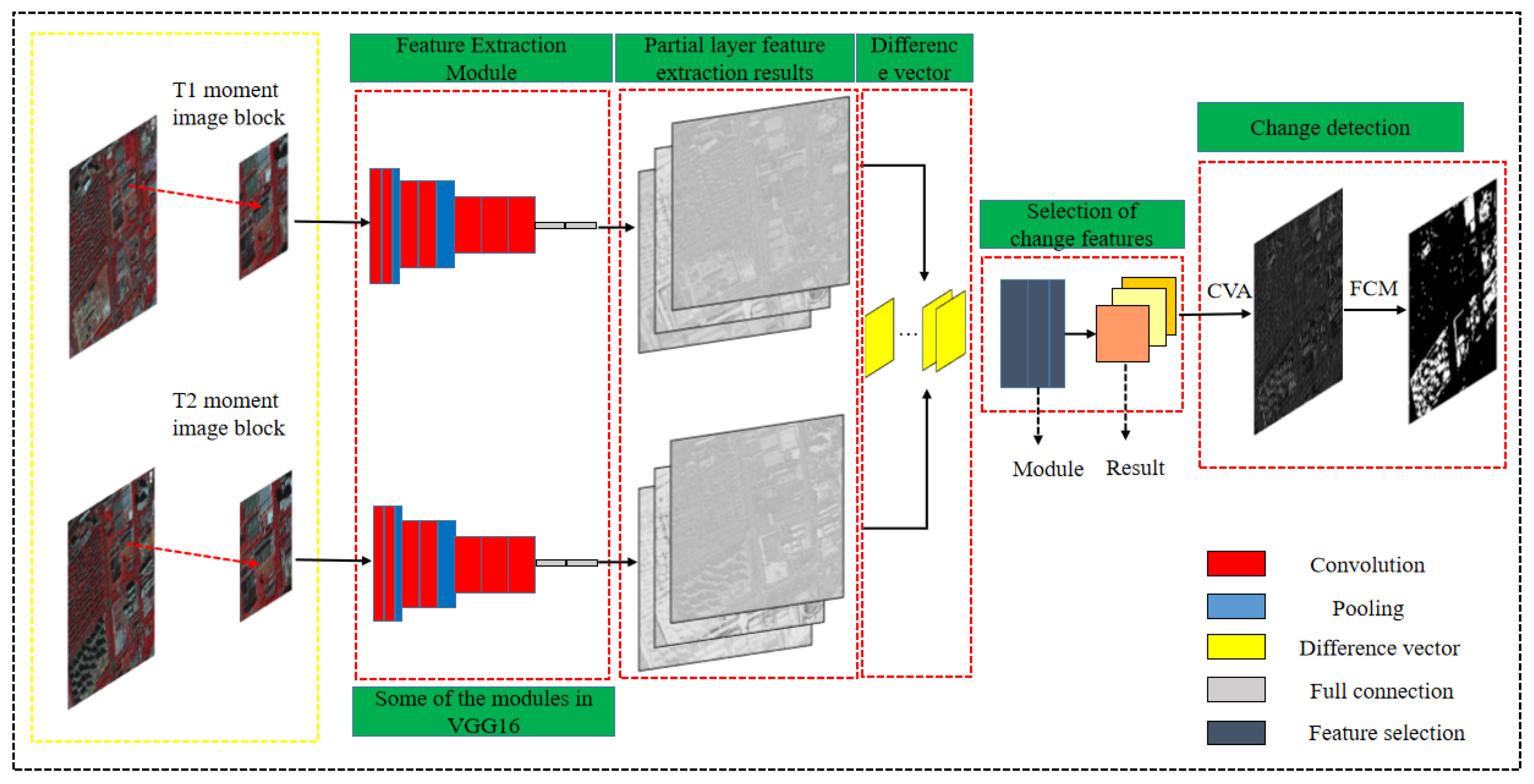
The proposed TL-FS method and the network architecture are illustrated in Figure 1. Firstly, the convolutional layers of the first three scales from the VGG16 model are utilized for feature extraction from the input VHR remote sensing images. Secondly, the designed variance-based feature selection algorithm is embedded into the overall internal structure for selecting features from all deep image features. Next, the selected change features of multitemporal VHR images are combined and differenced, with the CVA used to compute the magnitude of the difference vectors. Finally, the FCM algorithm is employed to obtain the binary change detection image.

Figure 1.
Flowchart of the TL-FS method.
2.1. Deep Feature Learning
CNNs are multilayer deep architectures capable of capturing complex visual features in remote sensing images. The objective of this study is to effectively utilize the multilayer characteristics of CNNs to extract features relevant for change detection. To achieve this goal, the preprocessed images are first input into a pretrained CNN model, and deep features from multiple temporal images are extracted from certain layers of the CNN. A CNN is composed of numerous layers, and each layer consists of many features that learn various visual concepts from the input images [26]. Here arises the following challenge: how to design a change detection framework leveraging the advantageous characteristics of CNNs. Utilizing only a pretrained feature extraction network is insufficient for effectively and accurately performing change detection tasks. It is also necessary to select an appropriate pretrained CNN and specific feature extraction layers. The main challenge in designing the framework is integrating the CNN model with the change detection process.
For the proposed TL-FS framework, any architecture can be chosen as the feature extractor for the model, and it can output feature information for each pixel in the remote sensing images. Indeed, features can be obtained from each layer, but the performance of these features depends on each layer. In the initial layers of a CNN, low-level visual features are learned, such as colors commonly encountered and edge features of images. As the network delves deeper, it learns higher-level visual concepts by combining the low-level features extracted previously. These more complex visual concepts are highly beneficial for analyzing intricate VHR images. However, as the model goes deeper, its generalization ability to new input features decreases, and it also lacks spatial correlation [38]. Features obtained from multiple layers of a CNN are more effective than those from a single layer because a CNN can learn at multiple scales. Finally, features from multiple layers are combined to form a set of feature vectors.
2.2. Feature Extraction
CNN feature extraction differs from traditional feature extraction methods. Some traditional feature extraction techniques cannot comprehensively extract features from VHR images, such as traditional spectral-based and texture-based methods. Although some methods can reduce the dimensionality of features, they may also lose information about ground objects, making it difficult to handle images in complex scenes. CNNs progress from local features to global features and from low-level features to high-level features, which can be highly abstract and conceptual, closer to the principles of human vision. Therefore, CNNs have found wider applications in image processing [39].
In an ideal scenario, when conducting change detection with neural networks, a large number of pixel-level annotated samples are required. These samples assist in training the current network to accurately identify change detection areas in multitemporal remote sensing images. However, the image properties of VHR remote sensing images differ from natural images. They have different resolutions, imaging modes, and different sensor types. This complexity in VHR images results in the difficulty of obtaining high-quality pixel-level samples. If a simple labeling method is employed, the model may lack a comprehensive understanding of the complexity of VHR images, which could affect both the feature extraction process and the change detection process [40].
Therefore, the feature extraction method in this paper is based on the idea of transfer learning, utilizing a dual-channel structure based on VGG16 to address the issue of insufficient training samples. It extracts multi-scale and multi-depth feature maps from X1 and X2. The selected pretrained network was trained on the AID aerial dataset, with 9500 training samples and 500 validation samples. The image size is 600 × 600 with a resolution of 0.5 m [41]. The original VGG16 architecture has five max-pooling layers, indicating five different scales of convolutional layers. To consider the size of the feature maps, we utilize the convolutional layers from three scales of the VGG16 for feature extraction experiments. Some selected parts of the VGG16 architecture information are shown in Table 1. To consider the size of the image, seven convolutional layers are selected for feature extraction. Each convolutional layer computes features at different depths. These seven convolutional layers are named conv1, conv2, conv3, conv4, conv5, conv6, and conv7. The input to this network requires support for the three channels of red (R), green (G), and blue (B). For the input raw images, different datasets have different sizes, while the VGG16 model has a fixed image input size of 224 × 224 pixels. Therefore, as input data, the images are cropped into multiple 224 × 224-sized image blocks with a stride of 100 pixels, which are then fed into the feature extraction module.

Table 1.
Detailed information on the used feature extraction module. The number after/in the kernel size represents the stride.
2.3. Variance Feature Selection Strategy
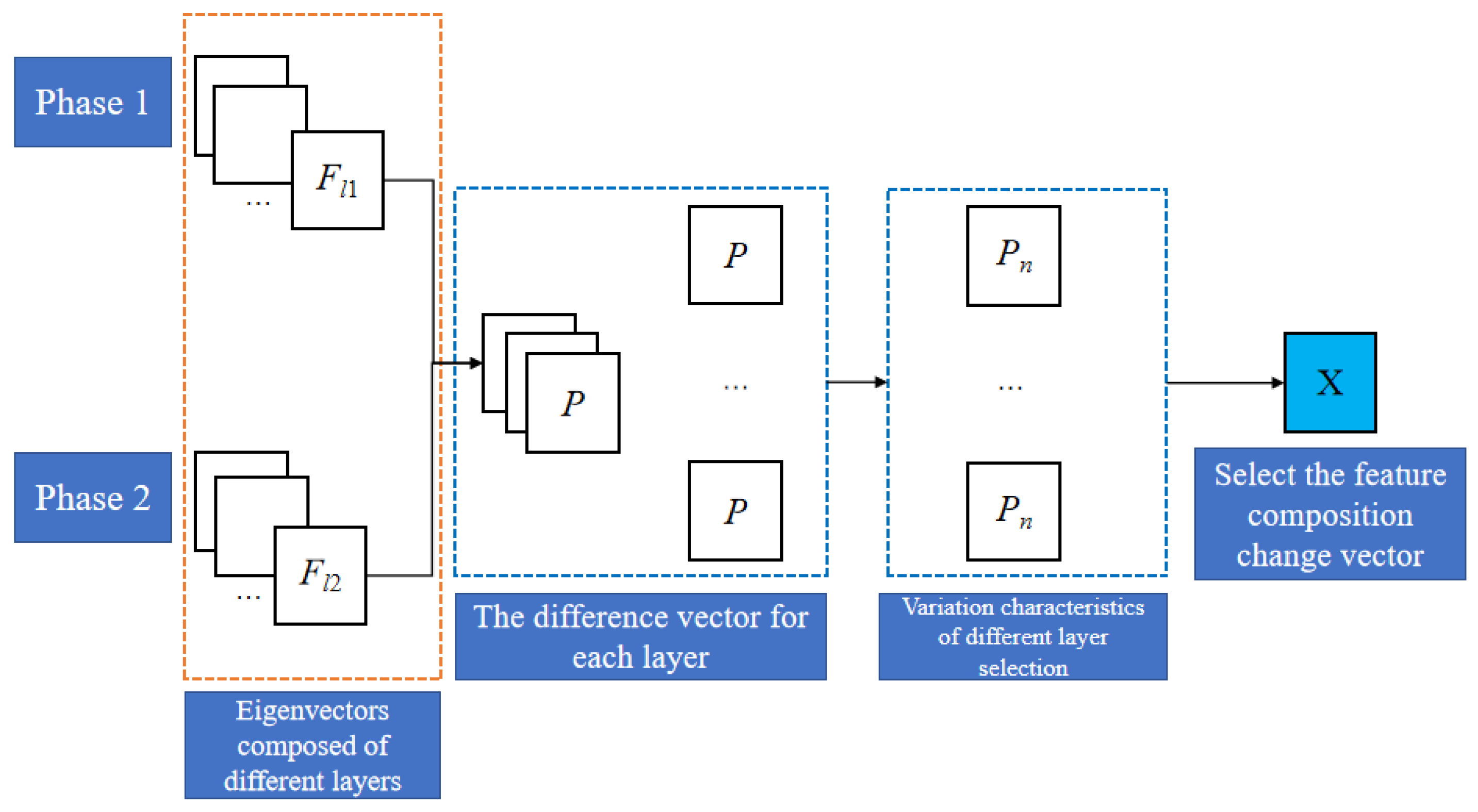
For VHR image change detection, during transfer learning, many irrelevant changes affect the model’s performance, necessitating a method to urgently filter out these change features [35,36]. By employing a variance-based selection method embedded into the model to address the poor performance caused by feature redundancy, the proposed feature selection strategy is depicted in Figure 2. Assume that the total number of feature layers of the total model is L. If L has a subset l, l∈L. After the selection of the change difference features, all selected features related to the changes will form a vector, which is named X, where X represents the difference features of the bi-temporal image.
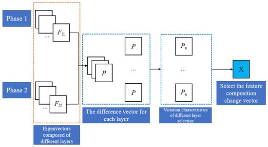
Figure 2.
The process of feature selection variation.
Let Fl1 and Fl2 be the features corresponding to subset l. Subtracting them yields the difference vector P, as follows:
Suppose there exists Pn, which is a subset of P with Pn∈P. Pn contains all of the selected features related to changes. At this point, in order to calculate Pn, the variance is used as an index to filter the relevant change features, and the variance is used as a sensitivity index of the change information. It is important to note that the features containing information related to changes have higher variability compared to features unrelated to change. This implies that feature values undergo strong variations between changing and unchanged pixels. During the change feature selection process, the proposed method is unsupervised. Therefore, it is necessary to divide the difference vectors P of all features in l into K parts. For any part k where k in K, we calculate the variance S2(P) of P and arrange the variances of all computed features in descending order. The selected features are chosen according to a certain ratio. Therefore, all selected features Pn in layer l are as follows:
In the formula, plk represents all features of the k-th part in layer l, where plk∈P. By combining and arranging Pn, we obtain X, where the range of n is n∈(1, N), and N is the number of selected change features. Therefore, the sought-after vector of selected change features X is as follows:
2.4. Binary Change Detection
For the change feature vector X, obtained using the selection strategy proposed in Section 2.3, the CVA algorithm [14] is employed to distinguish between change and no-change pixels in VHR images. The change intensity V for all pixels in the image is calculated as follows:
After calculating the intensity image, any available clustering algorithm or threshold segmentation method can be used for binary change detection to obtain the change detection map. The quality of segmentation depends on the accuracy of the produced change intensity values. Therefore, the Fuzzy C-Means (FCM) clustering algorithm [37] is selected to classify the image into the following two categories: change and no change.
In Equation (5), T(g, h) denotes the pixel point of the image pixel in row g and column h, c denotes the point identified as changed, u denotes the point identified as unchanged, M denotes the central value of the feature intensity, and the final binary change map is obtained by distinguishing between changed and unchanged pixels.
3. Results and Experiments
3.1. Datasets
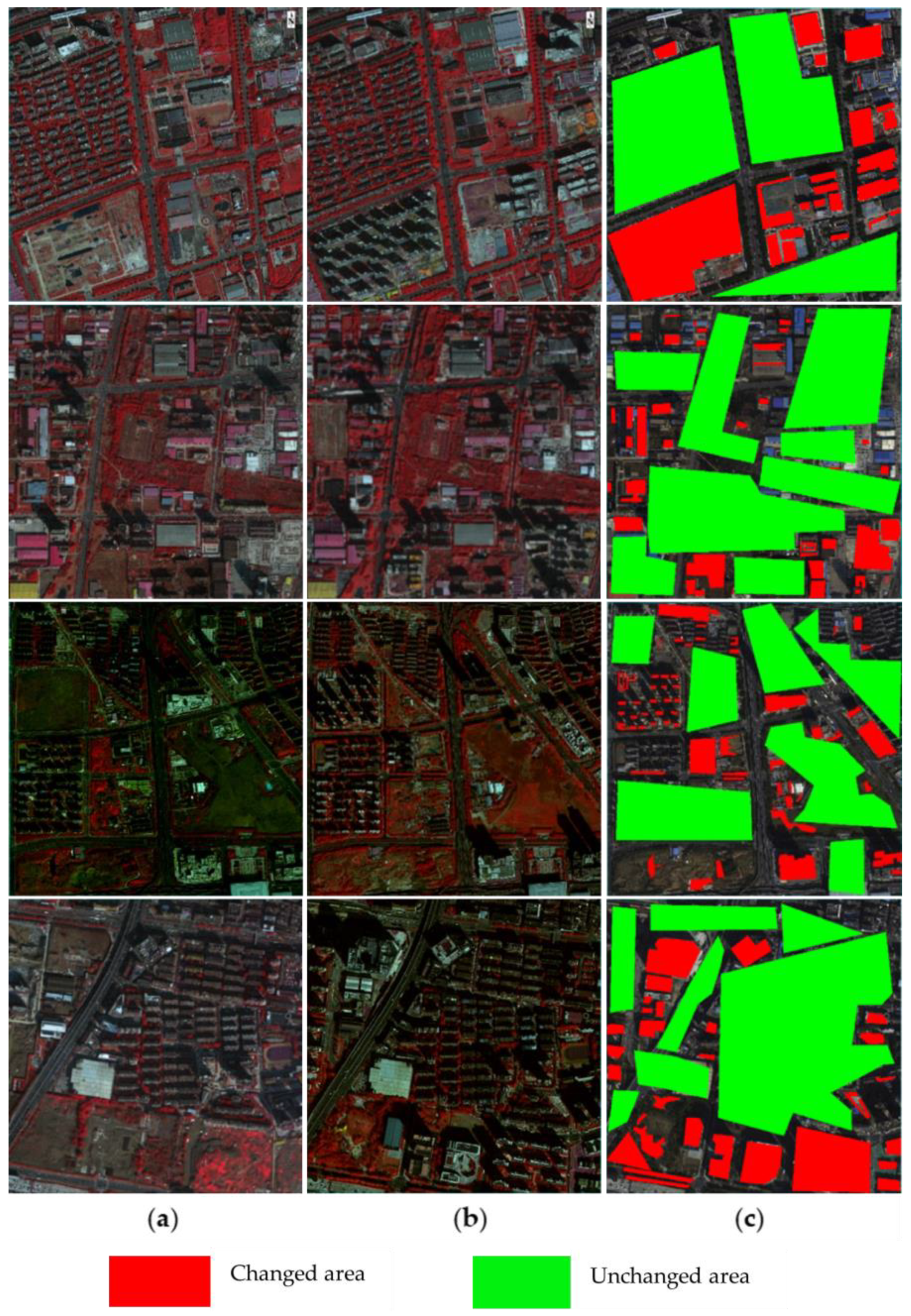
To validate the effectiveness of the proposed method in addressing feature redundancy and improving transfer learning for change detection, we conducted experiments on four Beijing-2 VHR image datasets, named A, B, C, and D. The images consist of dual-temporal data from 2018 and 2021 in the Binhu New Area of Hefei City, as depicted in Figure 3a,b. Figure 3 illustrates the four VHR optical image datasets used for method validation. The land cover types in datasets A and B only include vegetation and impervious surfaces, while datasets C and D contain bare soil, vegetation, and impervious surfaces. The sizes of the four image datasets are as follows: 1500 × 1500, 1600 × 1600, 2000 × 2000, and 1000 × 1000 pixels, respectively. The resolution of the Beijing-2 images is 0.8 m for panchromatic and 3.2 m for multispectral bands. The datasets used are fusion images of panchromatic and multispectral data.
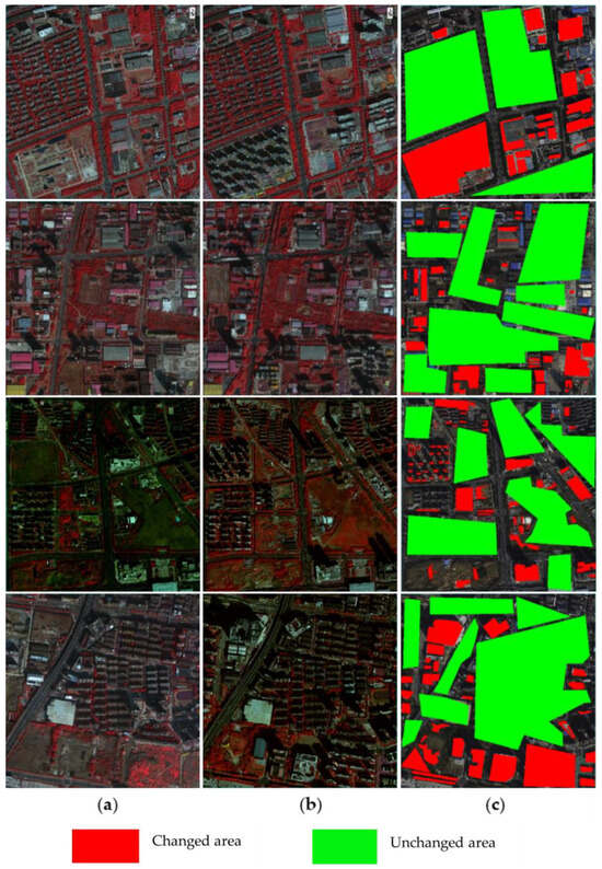
Figure 3.
The four datasets used in the experimentations named A, B, C, and D; (a–c) the prechange images, postchange images, and the standard reference change maps generated through visual interpretation, respectively.
3.2. Experimental Procedure
All of the experiments on the datasets were conducted on Intel Core i7-11800H CPU @ 2.3 GHz (32 GB RAM) with GPU model NVIDIA GeForce Experience 3060. The experiments were conducted using five change detection methods for comparison, which are CVA, IRMAD, Principal Component Analysis combined with K-means clustering (PCA-Kmeans), Deep Slow Feature Analysis (DSFA) [42], and Scale and Relation Aware Siamese Network (SARAS-Net) [43]. The first three of these are traditional change detection algorithms, and the last two are deep learning-based change detection methods. Like the proposed method, DSFA also uses the CVA and FCM clustering algorithms to obtain the change map. In order to compare it with the results of the model itself, in the subsequent discussion, we also conducted ablation experiments on the model to evaluate the performance of the change feature selection module. Precision, recall, F1-score, and Overall Accuracy (OA) are used to assess accuracy.
In Equations (6) through (9), TP represents true positive, indicating pixels that are actually changed and predicted as changed; FP represents false positive, indicating pixels that are actually unchanged but predicted as changed; FN represents false negative, indicating pixels that are actually changed but predicted as unchanged; TN represents true negative, indicating pixels that are actually unchanged and predicted as unchanged.
3.3. Experimental Results
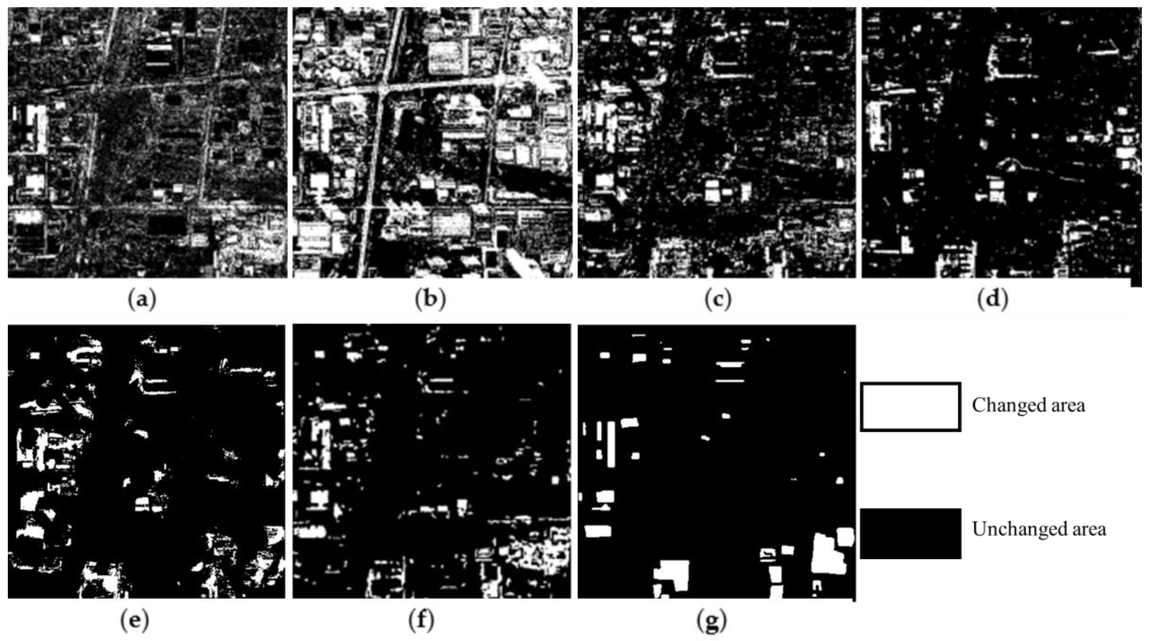
In dataset A, comparing the standard reference change map in Figure 4g with Figure 4a–f, it can be seen that the CVA, IRMAD, PCA-Kmeans, DSFA, and SARAS-Net algorithms have larger areas of false detections and missed detections of vegetation and impervious surface changes. However, the TL-FS proposed in this paper is closer to the standard in the detection of the change region, and the relative error is smaller.
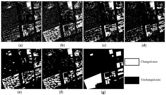
Figure 4.
The change detection results of the different methods on dataset A: (a–g) CVA, IRMAD, PCA-Kmeans, DSFA, SARAS-Net, TL-FS, and standard reference change map, respectively.
In dataset B, comparing the standard reference change map in Figure 5g with Figure 5a–f, it can be seen that CVA and IRMAD misdetected numerous invariant regions and are not suitable for change detection on vegetation and impervious surfaces. While PCA-Kmeans, DSFA, and SARAS-Net detected slightly better relative to the first two algorithms, they still have more missed regions compared to TL-FS, which remains the closest to the standard reference.
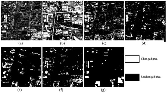
Figure 5.
The change detection results of the different methods on dataset B: (a–g) CVA, IRMAD, PCA-Kmeans, DSFA, SARAS-Net, TL-FS, and standard reference change map, respectively.
In dataset C, comparing the standard reference change map in Figure 6g with the change detection maps in Figure 6a–e, it can be found that CVA, IRMAD, and PCA-Kmeans consistently exhibited incomplete detections of changes in the buildings and omissions of changes in bare soil, which led to significant detection errors. On the other hand, DSFA, SARAS-Net, and TL-FS showed more accurate detection results with a smaller range of false detections and omissions.
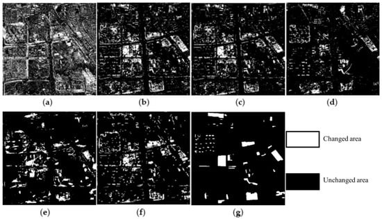
Figure 6.
The change detection results of the different methods on dataset C: (a–g) CVA, IRMAD, PCA-Kmeans, DSFA, SARAS-Net, TL-FS, and standard reference change map, respectively.
In dataset D, comparing the standard reference change map in Figure 7g with the change detection maps in Figure 7a–e, it can be found that the detection performances of CVA and IRMAD for changes in bare soil, vegetation, and impervious surfaces were poor. Although the detection accuracies of PCA-Kmeans, DSFA, and SARAS-Net improved, there were still more false detection areas, and there remains an obvious gap with TL-FS.
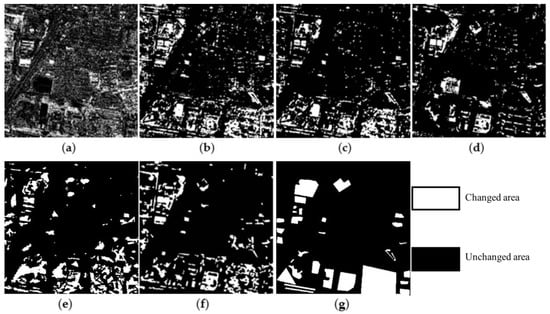
Figure 7.
The change detection results of the different methods on dataset D: (a–g) CVA, IRMAD, PCA-Kmeans, DSFA, SARAS-Net, TL-FS, and standard reference change map, respectively.
Figure 4, Figure 5, Figure 6 and Figure 7 display the change detection results for datasets A, B, C, and D using the following six different algorithms: CVA, IRMAD, PCA-Kmeans, DSFA, SARAS-Net, and TL-FS. Compared to the standard reference change map in Figure 3c, the CVA, IRMAD, PCA-Kmeans, DSFA, and SARAS-Net detection results consistently exhibited incomplete detection of building changes and omissions in vegetation changes. The proposed TL-FS method demonstrated a higher change detection accuracy, with significantly smaller areas of false detections and omissions. Overall, the proposed method outperforms the other methods in various aspects. Firstly, in the results from the CVA and IRMAD, not only do numerous errors appear, but these methods also failed to utilize deep features in the VHR images. Consequently, the application of the CVA algorithm to the VHR images resulted in severe salt-and-pepper noise. This phenomenon indicates that using only spectral features is not feasible in complex urban VHR scenes. The change maps produced by the PCA-Kmeans method show a reduction in salt-and-pepper noise due to the consideration of contextual information. However, the performance of this algorithm is not robust, leading to inconsistent results across different datasets and scenes. In the change detection results obtained using the DSFA method, we can observe that although DSFA is an improvement based on the SFA algorithm and utilizes two deep networks for computation, its performance is still suboptimal. This is because the algorithm does not perform change feature selection among multitemporal remote sensing images. SARAS-Net introduces a variety of modules, such as scale-aware and relationship-aware modules, which increases the complexity of the network, and its training model needs to be adjusted in a targeted manner for the change patterns of different urban areas, leading to an increased risk of model overfitting, and the network may not perform as well as expected for complex urban areas with more complicated change patterns.
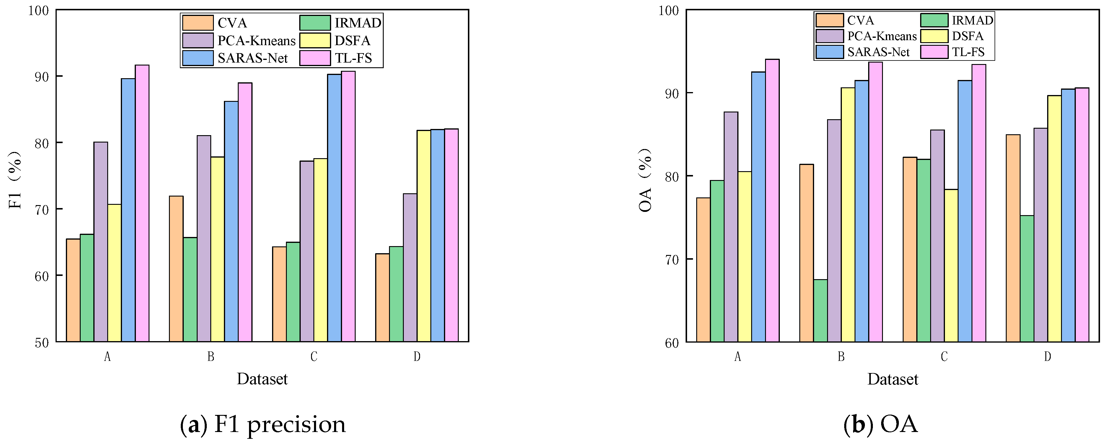
It can be seen from Table 2 that the precision of TL-FS was the highest, indicating that compared with CVA, IRMAD, PCA-Kmeans, DSFA, and SARAS-Net, our proposed model has a stronger ability to identify the changing regions and can more accurately identify which regions have substantial changes. The recall of TL-FS was higher than that of the other five models on Datasets A, B, and C and slightly lower on Dataset D, but the F1-score was higher than that of the other models, indicating that its overall comprehensive performance was stronger. Figure 8 shows the F1 and OA values of all methods, from which we can see that the F1 and OA values of TL-FS are higher than those of the other five models, indicating that the model achieved a good balance between the accuracy rate and recall rate, could correctly classify most pixels or regions in the image, as well as effectively identify the changed parts. At the same time, the running time of TL-FS is shorter than that of other models, indicating that our proposed model not only guarantees a high-precision change detection capability but also has the advantage of fast response, which is suitable for application scenarios requiring real-time performance and high accuracy.

Table 2.
The accuracy values of different methods for datasets A–D.
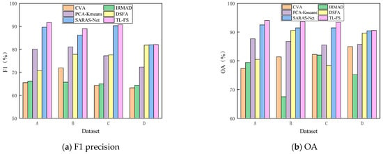
Figure 8.
Comparison of the accuracy verification results of different change detection methods.
Here, we take F1-scores as examples. On the first dataset, the F1 value of the TL-FS method we proposed is 91.64%, which is 26.16%, 25.05%, 11.06%, 20.98%, and 2.05% higher than those of CVA, IRMAD, PCA-Kmeans, DSFA, and SARAS-Net, respectively. On the second dataset, the F1 value of the proposed method is 88.95, which is 17.04%, 23.27%, 7.93%, 11.14%, and 2.77% higher than those of CVA, IRMAD, PCA-Kmeans, DSFA, and SARAS-Net, respectively. On the third dataset, the F1 of the proposed method is 90.69%, which is 26.41%, 25.69, 13.50%, 13.15%, and 0.44% higher than those of CVA, IRMAD, PCA-Kmeans, DSFA, and SARAS-Net, respectively. On the fourth dataset, the F1 value of the proposed method is 82.01, which is 18.77%, 17.67%, 9.75%, 0.21%, and 0.08% higher than those of CVA, IRMAD, PCA-Kmeans, DSFA, and SARAS-Net, respectively.
4. Discussion
4.1. Necessity of Change Feature Selection
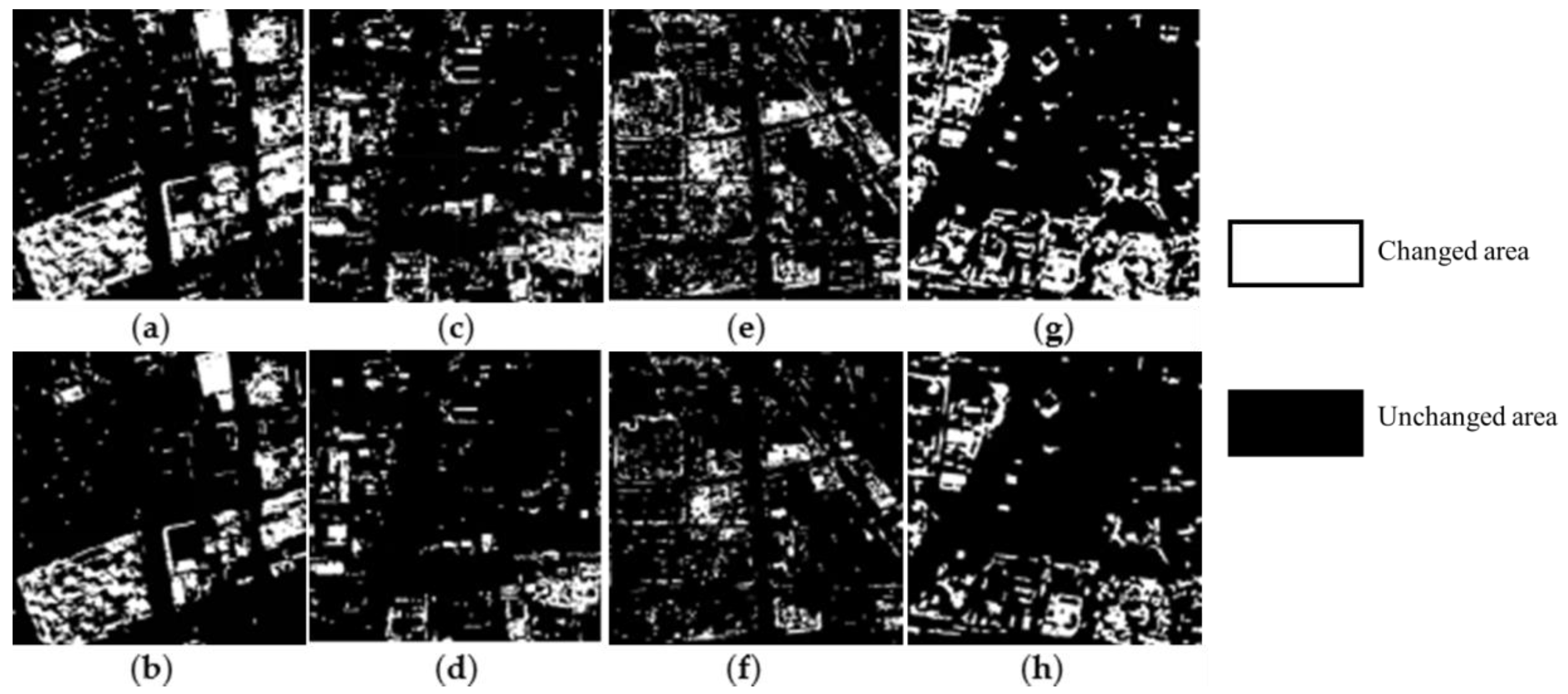
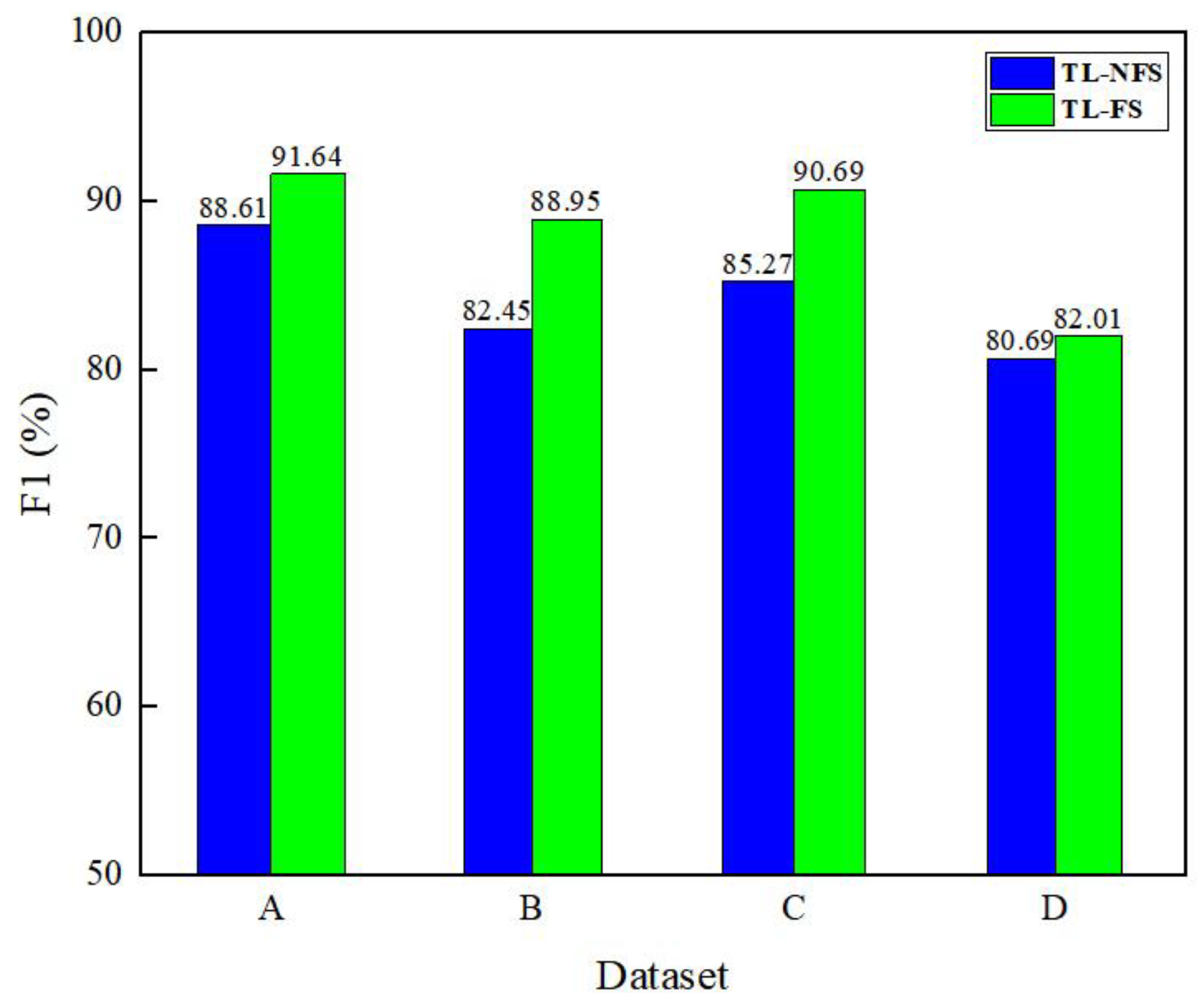
In change detection experiments, most networks extract image features based on a single image without considering the spatial correlations among multiple images. This oversight leads to feature redundancy when using deep learning models for change detection, resulting in inefficient use of computational resources, increased processing time, and suboptimal detection results. Here, we intend to demonstrate the necessity of the feature selection module (FS) through ablation experiments. The method without the feature selection module is named TL-NFS, while the proposed method with the feature selection module is named TL-FS. The resulting images for both methods are shown in Figure 9, and the accuracy statistics are depicted in Figure 10. From the statistical graph, it can be observed that the F1-score improved by 3.03%, 6.50%, 5.42%, and 1.32% across the four datasets. Regardless of the dataset, the proposed TL-FS method consistently achieves higher F1-scores, indicating better performance.
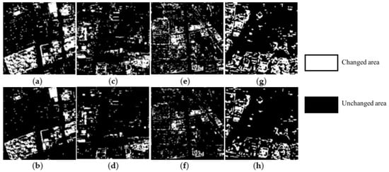
Figure 9.
Comparison of TL-FS and TL-NFS change detection results: (a,b), (c,d), (e,f), and (g,h), respectively, represent the results of datasets A, B, C, and D with and without the FS module.

Figure 10.
Comparison of F1-scores between TL-FS and TL-NFS.
4.2. The Role of the Feature Variance Algorithm
Transfer learning models can capture a wide range of deep features that represent land cover information. However, the deep features computed from bi-temporal images often include irrelevant changes, which can adversely affect change detection. As described in Section 2.3, the absolute values of the differences in unchanged features tend to approach zero, while the differences in the changed features deviate significantly from zero, displaying substantial variability. Variance can serve as a sensitivity indicator for change information, with the variance in the change regions being markedly higher than that in unchanged regions [35,36]. Therefore, relevant change features can be effectively filtered based on their variance values, enhancing the sensitivity of the proposed change detection model to urban area change information.
4.3. Analysis of Features Extraction Results from Different Layers
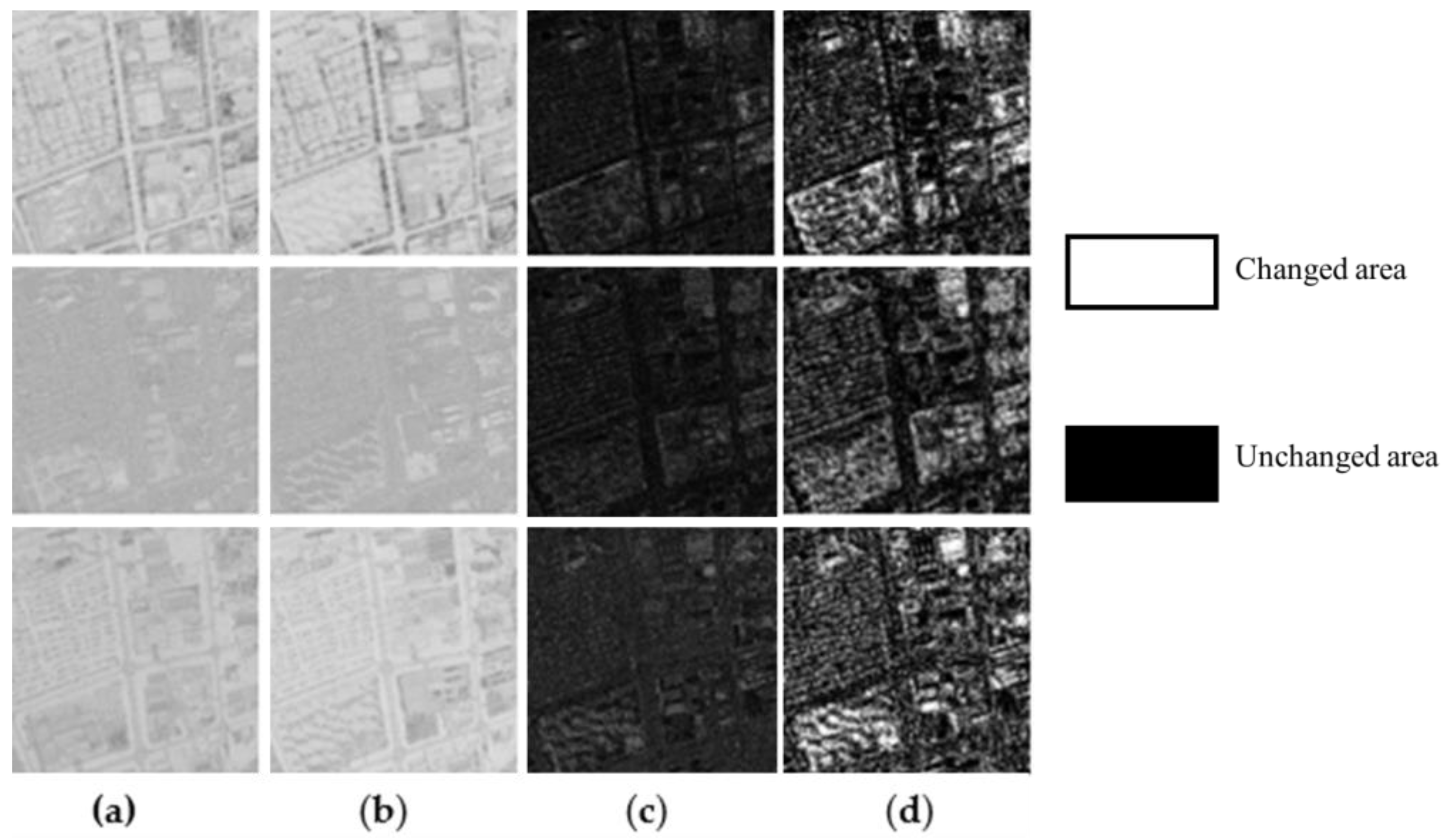
Here, taking the feature extraction results of the first dataset as an example, each layer of the CNN learns many features, with the features learned in the initial layers being closer to the original image. The features in the subsequent layers continue to build upon those learned in the previous layers, progressing in a hierarchical fashion. The feature extractor in the TL-FS framework proposed in this paper is part of the VGG-16 architecture. Here, the results are displayed by selecting the layers conv2, conv4, and conv7. As shown in Figure 11, it is unreasonable to represent the entire complex urban area using features from a single layer. Each layer exhibits the following different characteristics: conv2, being closer to the original image, tends to blur and produce false alarms around the edges of building structures; conv4, being deeper, learns more abstract features, but some vegetation-related information may not be adequately represented; and despite being the deepest layer used, conv7 exhibits lower accuracy in detecting the boundaries of various urban features, likely due to its implicit reduction in spatial precision. The TL-FS method, by selecting features from each layer and composing a vector containing only changed features, can better utilize the change information from each layer. Consequently, it can provide more precise boundary information for each changed object and eliminate a considerable amount of noise caused by irrelevant change features.

Figure 11.
Different layer feature analysis results (taking dataset A as an example): (a,b) urban feature extraction maps of conv2, conv4, and conv7 in the prechange and postchange phases, respectively; (c) feature difference maps of the three convolutional layers; (d) change maps of the three convolutional layers.
4.4. Comparison of the Results and Running Time of TL-FS Method
4.4.1. Discussion of Localized Test Results
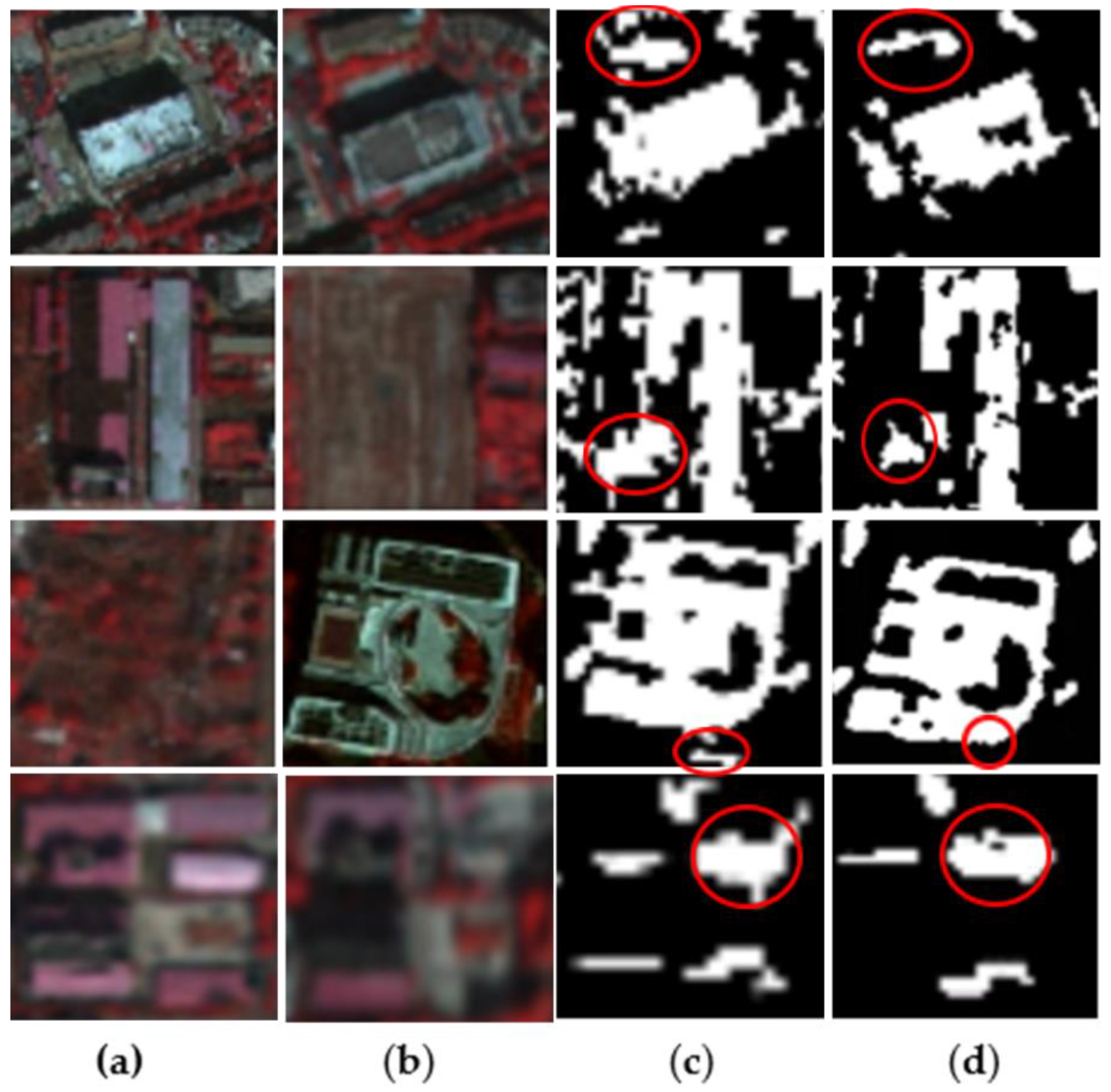
The transfer learning network based on the FS module exhibited a good detection performance when applied to VHR images in complex regions overall. For detailed illustrations, some excerpts from the datasets are presented in Figure 12.
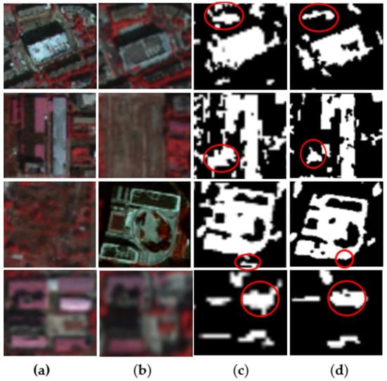
Figure 12.
Comparison of the results between TL-FS and TL-NFS: (a) parts of the four datasets in 2018; (b) parts of the four datasets in 2021; (c) change detection result graphs for TL-NFS; (d) change detection result graphs for TL-FS. The red circles indicate the difference in detail handling between TL-FS and TL-NFS.
From the highlighted red circles in the figures, we can observe that the detailed processing of TL-FS is better than TL-NFS. For certain buildings, the textures and shapes are clearer with TL-FS. And in the first set of examples, TL-NFS made errors in detecting vegetation, while TL-FS effectively captured the vegetation change information. Although the proposed method is influenced by unsupervised algorithms and may not perform well in discerning shadows, it exhibits better texture representation for buildings compared to TL-NFS. This is because the proposed change feature selection algorithm eliminates irrelevant change features from the multitemporal images, thus avoiding the influence of redundant features and yielding more accurate change detection results.
4.4.2. Running Time
Table 3 presents the runtime with and without the FS module, along with comparisons with the runtimes of the contrasted methods in Table 2, facilitating an assessment of whether adding the FS module is worthwhile. The results indicate that on all datasets, TL-FS had shorter runtimes compared to TL-NFS, and their change detection results show significant differences. Considering the improvements in performance and accuracy, adding the FS module is worthwhile.

Table 3.
Runtimes of the methods with and without the FS modules.
5. Conclusions
This paper proposes a novel method for change detection in complex urban areas, which can detect changes in dual-temporal remote sensing images without the need for high-quality labeled samples. Additionally, a change feature selection algorithm is designed to effectively connect “change information” with the model, addressing irregularities and false detections of buildings caused by feature redundancy in complex urban areas. Inspired by the variance selection strategy, computing the variance of change features and filtering them provides a transfer learning-based change detection approach for urban scenes.
In the context of performing change detection tasks using deep learning, unlike object recognition or classification, the abundance of features computed by each layer of the deep learning model can lead to feature redundancy, affecting the effectiveness of the detection process. In particular, an excessive presence of irrelevant change features can adversely impact the detection performance. To address the issues of unclear terrain textures, such as incomplete building structures caused by feature redundancy, and to enhance the efficiency of transfer learning models in change detection for urban VHR imagery, this paper proposes a transfer learning change detection model that integrates change feature selection.
By selecting deep change feature vectors related to the changes, this approach reduces computational complexity while achieving excellent change detection results in urban areas. The comparison experiments on four VHR datasets led to the following conclusions: TL-FS achieves good change detection results in urban areas without the need for samples and exhibits higher F1 values compared to some common methods. The designed change feature selection algorithm filters out redundant features unrelated to changes, thereby reducing computational complexity. Compared to transfer learning models without change feature selection, TL-FS performs better in detecting certain buildings, resulting in clearer textures and more complete edge shapes. The experimental results demonstrate that TL-FS is effective for change detection in complex urban areas.
The change detection model proposed in this paper is derived from unsupervised algorithms, requiring no training samples. It achieves satisfactory detection results on urban areas. However, the designed method can only detect one type of change, whereas urban planning and development often require not only identifying changing areas but also understanding the types of changes occurring. Therefore, as a future direction, a more comprehensive framework for detecting multiple types of urban changes could be developed by integrating the proposed TL-FS model with change magnitude thresholds.
Author Contributions
Conceptualization, Q.C. and P.Y.; methodology, P.Y.; software, P.Y.; validation, Q.C. and P.Y.; formal analysis, S.C. and P.Y.; investigation, Q.C.; resources, Q.C.; data curation, P.Y.; writing—original draft preparation, P.Y.; writing—review and editing, Y.X., Y.L. and L.Z.; visualization, Q.C. and J.L.; supervision, Y.X.; project administration, J.L.; funding acquisition, Q.C. All authors have read and agreed to the published version of the manuscript.
Funding
This research was funded by both the National Key R&D Plan of China, under grant numbers: 2022YFC3004404 and 2023YFF1305303, and the National Natural Science Foundation (NSFC) of China, under grant number: 42271478.
Data Availability Statement
The data that support the findings of this study are available from the author upon reasonable request.
Acknowledgments
The authors express gratitude to Changguang Satellite Technology Co., Ltd., and China 21st Century Space Technology Application Co., Ltd., for providing Beijing 2 satellite images.
Conflicts of Interest
The authors declare no conflicts of interest.
References
- Singh, A. Review article digital change detection techniques using remotely-sensed data. Int. J. Remote Sens. 1989, 10, 989–1003. [Google Scholar] [CrossRef]
- Xian, G.; Homer, C.; Fry, J. Updating the 2001 National Land Cover Database land cover classification to 2006 by using Landsat imagery change detection methods. Remote Sens. Environ. 2009, 113, 1133–1147. [Google Scholar] [CrossRef]
- Coppin, P.; Lambin, E.; Jonckheere, I.; Muys, B. Digital change detection methods in natural ecosystem monitoring: A review. J. Int. J. Remote Sens. 2004, 25, 1565–1596. [Google Scholar] [CrossRef]
- Li, H.; Xiao, G.; Xia, T.; Tang, Y.Y.; Li, L. Hyperspectral image classification using functional data analysis. IEEE Trans. Cybern. 2013, 44, 1544–1555. [Google Scholar]
- Lu, X.; Yuan, Y.; Zheng, X. Joint dictionary learning for multispectral change detection. IEEE Trans. Cybern. 2016, 47, 884–897. [Google Scholar] [CrossRef] [PubMed]
- Wen, D.; Huang, X.; Bovolo, F.; Li, J.; Ke, X.; Zhang, A.; Benediktsson, J.A. Change detection from very-high-spatial-resolution optical remote sensing images: Methods, applications, and future directions. IEEE Geosci. Remote Sens. Mag. 2021, 9, 68–101. [Google Scholar] [CrossRef]
- Shafique, A.; Cao, G.; Khan, Z.; Asad, M.; Aslam, M. Deep learning-based change detection in remote sensing images: A review. Remote Sens. 2022, 14, 871. [Google Scholar] [CrossRef]
- Liang, S.; Yu, M.; Lu, W.; Ji, X.; Tang, X.; Liu, X.; You, R. A lightweight vision transformer with symmetric modules for vision tasks. Intell. Data Anal. 2023, 27, 1741–1757. [Google Scholar] [CrossRef]
- Asokan, A.; Anitha, J. Change detection techniques for remote sensing applications: A survey. Earth Sci. Inform. 2019, 12, 143–160. [Google Scholar] [CrossRef]
- Shi, W.; Zhang, M.; Zhang, R.; Chen, S.; Zhan, Z. Change detection based on artificial intelligence: State-of-the-art and challenges. Remote Sens. 2020, 12, 1688. [Google Scholar] [CrossRef]
- Lin, S.; Yao, X.; Liu, X.; Wang, S.; Chen, H.-M.; Ding, L.; Zhang, J.; Chen, G.; Mei, Q. MS-AGAN: Road Extraction via Multi-Scale Information Fusion and Asymmetric Generative Adversarial Networks from High-Resolution Remote Sensing Images under Complex Backgrounds. Remote Sens. 2023, 15, 3367. [Google Scholar] [CrossRef]
- Wang, L.; Li, R.; Zhang, C.; Fang, S.; Duan, C.; Meng, X.; Atkinson, P.M. UNetFormer: A UNet-like transformer for efficient semantic segmentation of remote sensing urban scene imagery. ISPRS J. Photogramm. Remote Sens. 2022, 190, 196–214. [Google Scholar] [CrossRef]
- Hussain, M.; Chen, D.; Cheng, A.; Wei, H.; Stanley, D. Change detection from remotely sensed images: From pixel-based to object-based approaches. ISPRS J. Photogramm. Remote Sens. 2013, 80, 91–106. [Google Scholar] [CrossRef]
- Malila, W.A. Change vector analysis: An approach for detecting forest changes with Landsat. In Proceedings of the LARS Symposia, West Lafayette, IN, USA, 1 January 1980; p. 385. [Google Scholar]
- Chen, J.; Lu, M.; Chen, X.; Chen, J.; Chen, L. A spectral gradient difference based approach for land cover change detection. ISPRS J. Photogramm. Remote Sens. 2013, 85, 1–12. [Google Scholar] [CrossRef]
- Fung, T.; LeDrew, E. Application of principal components analysis to change detection. Photogramm. Eng. Remote Sens. 1987, 53, 1649–1658. [Google Scholar]
- Canty, M.J.; Nielsen, A.A. Automatic radiometric normalization of multitemporal satellite imagery with the iteratively re-weighted MAD transformation. Remote Sens. Environ. 2008, 112, 1025–1036. [Google Scholar] [CrossRef]
- Chen, J.; Chen, X.; Cui, X.; Chen, J. Change vector analysis in posterior probability space: A new method for land cover change detection. IEEE Geosci. Remote Sens. Lett. 2010, 8, 317–321. [Google Scholar] [CrossRef]
- Praveen, B.; Parveen, S.; Akram, V. Urban Change Detection Analysis Using Big Data and Machine Learning: A Review. In Advancements in Urban Environmental Studies: Application of Geospatial Technology and Artificial Intelligence in Urban Studies; Rahman, A., Sen Roy, S., Talukdar, S., Shahfahad, Eds.; Springer International Publishing: Cham, Switzerland, 2023; pp. 125–133. [Google Scholar]
- Zhong, Y.; Ma, A.; soon Ong, Y.; Zhu, Z.; Zhang, L. Computational intelligence in optical remote sensing image processing. Appl. Soft Comput. 2018, 64, 75–93. [Google Scholar] [CrossRef]
- Ronneberger, O.; Fischer, P.; Brox, T. U-net: Convolutional networks for biomedical image segmentation. In Proceedings of the Medical Image Computing and Computer-Assisted Intervention–MICCAI 2015: 18th International Conference, Munich, Germany, 5–9 October 2015; Proceedings, Part III 18. 2015; pp. 234–241. [Google Scholar]
- Chen, L.-C.; Papandreou, G.; Schroff, F.; Adam, H. Rethinking Atrous Convolution for Semantic Image Segmentation. arXiv 2017, arXiv:1706.05587. [Google Scholar]
- Szegedy, C.; Liu, W.; Jia, Y.; Sermanet, P.; Reed, S.; Anguelov, D.; Erhan, D.; Vanhoucke, V.; Rabinovich, A. Going deeper with convolutions. In Proceedings of the IEEE Conference on Computer Vision and Pattern Recognition, Boston, MA, USA, 7–12 June 2015; pp. 1–9. [Google Scholar]
- LeCun, Y. LeNet-5, Convolutional Neural Networks. 2015. Available online: http://yann.lecun.com/exdb/lenet (accessed on 20 August 2023).
- Zahangir Alom, M.; Taha, T.M.; Yakopcic, C.; Westberg, S.; Sidike, P.; Shamima Nasrin, M.; Van Esesn, B.C.; Awwal, A.A.S.; Asari, V.K. The history began from alexnet: A comprehensive survey on deep learning approaches. arXiv 2018, arXiv:1803.01164. [Google Scholar]
- He, K.; Zhang, X.; Ren, S.; Sun, J. Deep residual learning for image recognition. In Proceedings of the IEEE Conference on Computer Vision and Pattern Recognition, Las Vegas, NV, USA, 27–30 June 2016; pp. 770–778. [Google Scholar]
- Khelifi, L.; Mignotte, M. Deep learning for change detection in remote sensing images: Comprehensive review and meta-analysis. IEEE Access 2020, 8, 126385–126400. [Google Scholar] [CrossRef]
- Liu, J.; Chen, K.; Xu, G.; Sun, X.; Yan, M.; Diao, W.; Han, H. Convolutional neural network-based transfer learning for optical aerial images change detection. IEEE Geosci. Remote Sens. Lett. 2019, 17, 127–131. [Google Scholar] [CrossRef]
- Andresini, G.; Appice, A.; Ienco, D.; Malerba, D. SENECA: Change detection in optical imagery using Siamese networks with Active-Transfer Learning. Expert Syst. Appl. 2023, 214, 119123. [Google Scholar] [CrossRef]
- Zhan, T.; Gong, M.; Jiang, X.; Zhao, W. Transfer learning-based bilinear convolutional networks for unsupervised change detection. IEEE Geosci. Remote Sens. Lett. 2021, 19, 8010405. [Google Scholar] [CrossRef]
- Habibollahi, R.; Seydi, S.T.; Hasanlou, M.; Mahdianpari, M. TCD-Net: A novel deep learning framework for fully polarimetric change detection using transfer learning. Remote Sens. 2022, 14, 438. [Google Scholar] [CrossRef]
- Song, A.; Choi, J. Fully convolutional networks with multiscale 3D filters and transfer learning for change detection in high spatial resolution satellite images. Remote Sens. 2020, 12, 799. [Google Scholar] [CrossRef]
- Li, N.; Wu, J. Remote sensing image detection based on feature enhancement SSD. In Proceedings of the 2023 35th Chinese Control and Decision Conference (CCDC), Yichang, China, 20–22 May 2023; pp. 460–465. [Google Scholar]
- Simonyan, K.; Zisserman, A. Very Deep Convolutional Networks for Large-Scale Image Recognition. arXiv 2014, arXiv:1409.1556. [Google Scholar]
- He, X.; Ji, M.; Zhang, C.; Bao, H. A variance minimization criterion to feature selection using laplacian regularization. IEEE Trans. Pattern Anal. Mach. Intell. 2011, 33, 2013–2025. [Google Scholar]
- He, X.; Cai, D.; Niyogi, P. Laplacian score for feature selection. In Proceedings of the 18th International Conference on Neural Information Processing Systems, Vancouver, BC, Canada, 5–8 December 2005; pp. 507–514. [Google Scholar]
- Bezdek, J.C.; Ehrlich, R.; Full, W. FCM: The fuzzy c-means clustering algorithm. Comput. Geosci. 1984, 10, 191–203. [Google Scholar] [CrossRef]
- Li, X.; Zhang, Y.; Cui, Q.; Yi, X.; Zhang, Y. Tooth-marked tongue recognition using multiple instance learning and CNN features. IEEE Trans. Cybern. 2018, 49, 380–387. [Google Scholar] [CrossRef]
- LeCun, Y.; Bengio, Y.; Hinton, G. Deep learning. Nature 2015, 521, 436–444. [Google Scholar] [CrossRef] [PubMed]
- Hou, B.; Wang, Y.; Liu, Q. Change detection based on deep features and low rank. IEEE Geosci. Remote Sens. Lett. 2017, 14, 2418–2422. [Google Scholar] [CrossRef]
- Xia, G.-S.; Hu, J.; Hu, F.; Shi, B.; Bai, X.; Zhong, Y.; Zhang, L.; Lu, X. AID: A benchmark data set for performance evaluation of aerial scene classification. IEEE Trans. Geosci. Remote Sens. 2017, 55, 3965–3981. [Google Scholar] [CrossRef]
- Du, B.; Ru, L.; Wu, C.; Zhang, L. Unsupervised deep slow feature analysis for change detection in multi-temporal remote sensing images. IEEE Trans. Geosci. Remote Sens. 2019, 57, 9976–9992. [Google Scholar] [CrossRef]
- Chen, C.-P.; Hsieh, J.-W.; Chen, P.-Y.; Hsieh, Y.-K.; Wang, B.-S. SARAS-net: Scale and relation aware siamese network for change detection. In Proceedings of the AAAI Conference on Artificial Intelligence, Washington, DC, USA, 7–14 February 2023; pp. 14187–14195. [Google Scholar]
Disclaimer/Publisher’s Note: The statements, opinions and data contained in all publications are solely those of the individual author(s) and contributor(s) and not of MDPI and/or the editor(s). MDPI and/or the editor(s) disclaim responsibility for any injury to people or property resulting from any ideas, methods, instructions or products referred to in the content. |
© 2024 by the authors. Licensee MDPI, Basel, Switzerland. This article is an open access article distributed under the terms and conditions of the Creative Commons Attribution (CC BY) license (https://creativecommons.org/licenses/by/4.0/).

