

Feature-Selection-Based Unsupervised Transfer Learning for Change Detection from VHR Optical Images

 ,
,  ,
,  ,
,
Abstract
1. Introduction
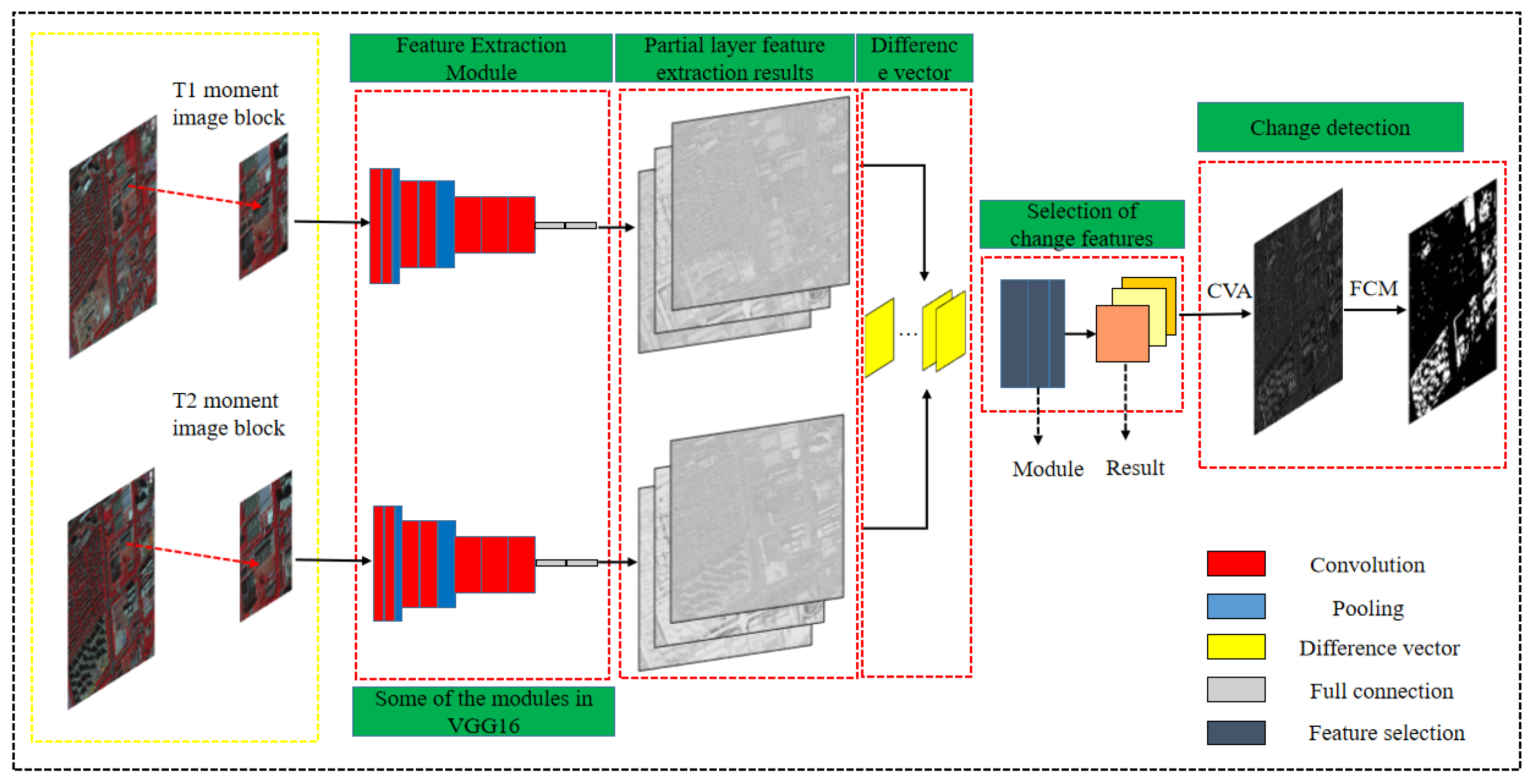
2. Methods
2.1. Deep Feature Learning
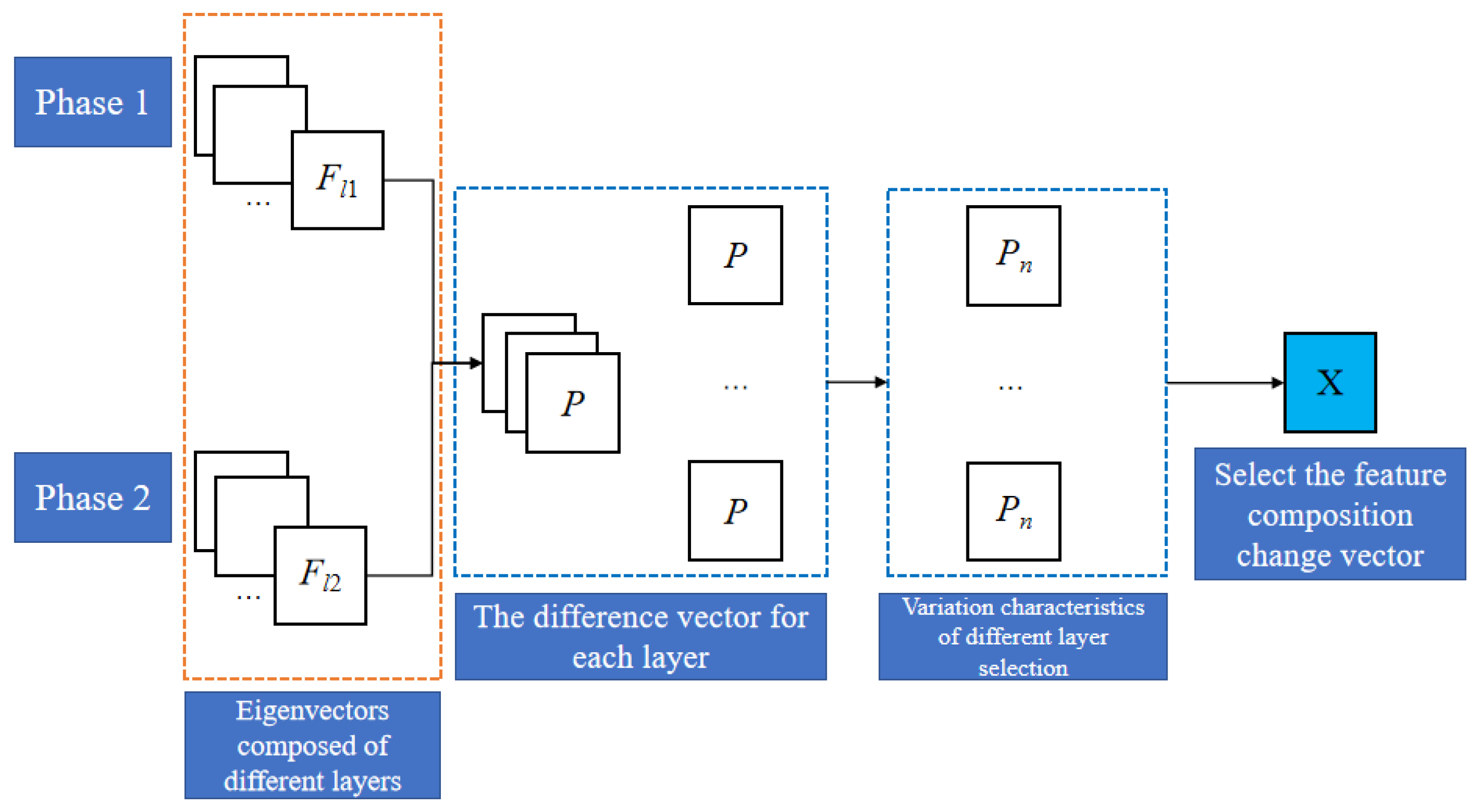
2.2. Feature Extraction
2.3. Variance Feature Selection Strategy
2.4. Binary Change Detection
3. Results and Experiments
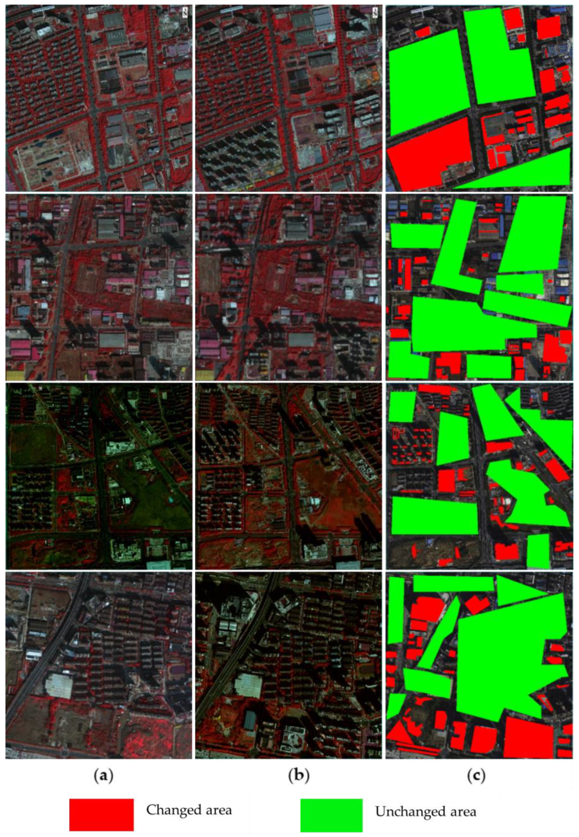
3.1. Datasets
3.2. Experimental Procedure
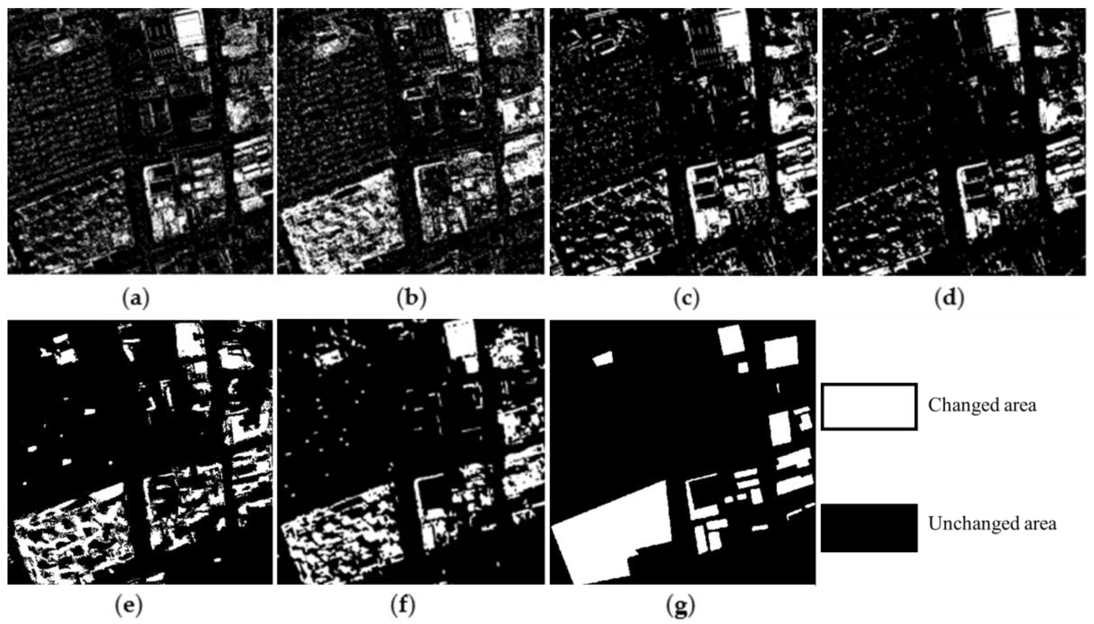
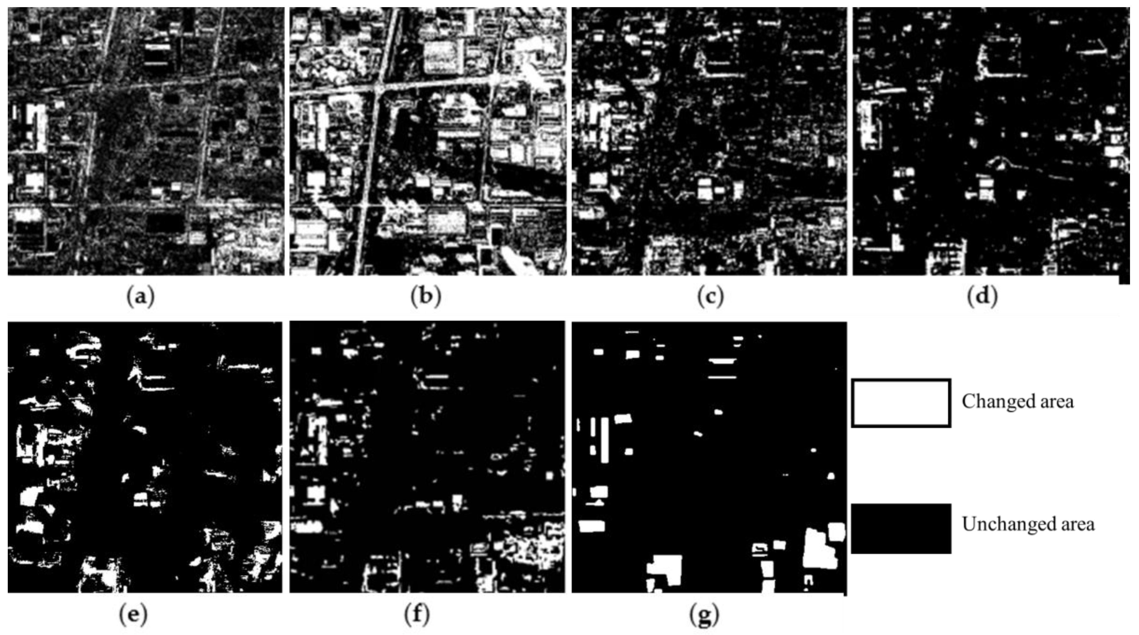
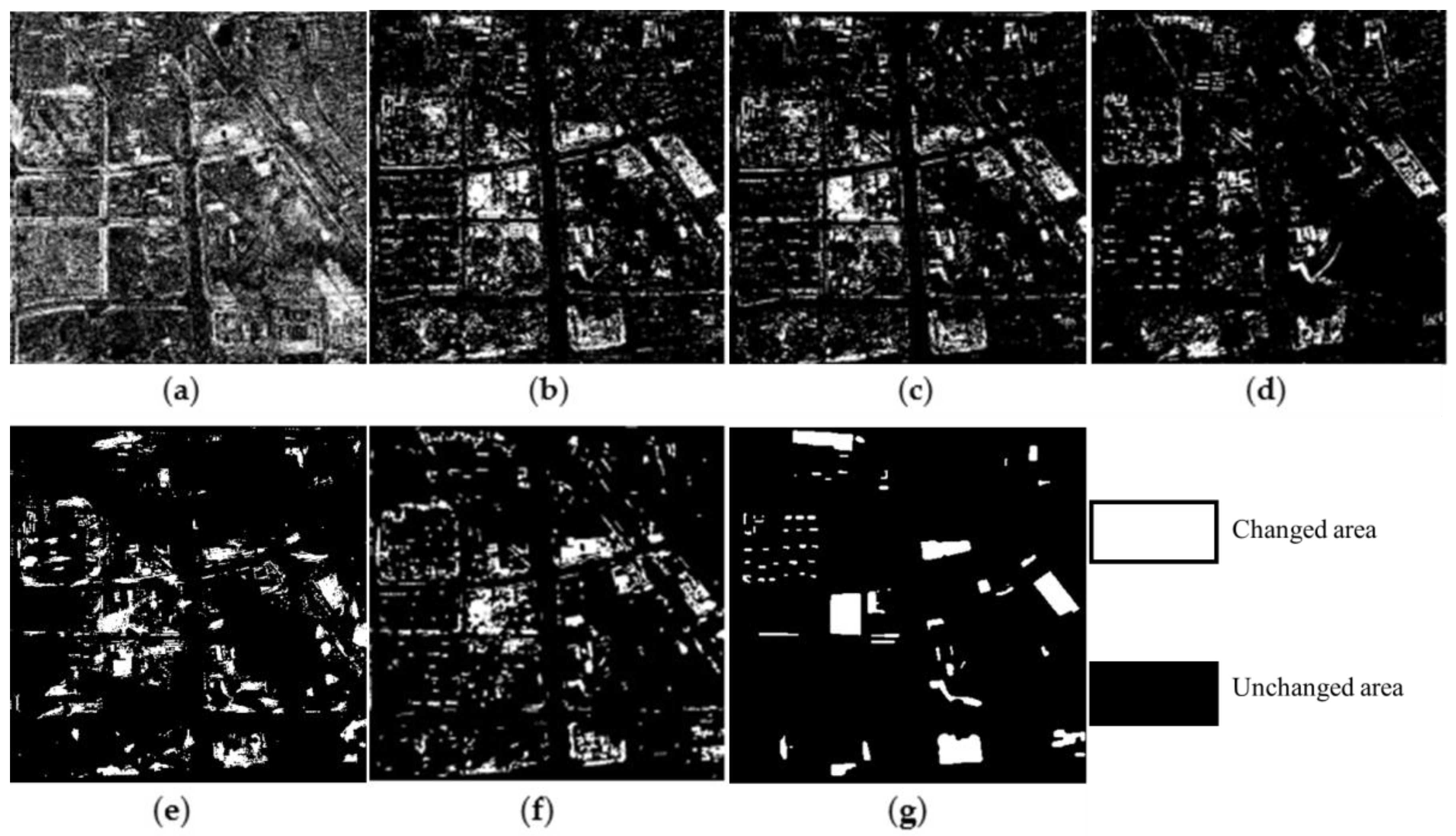
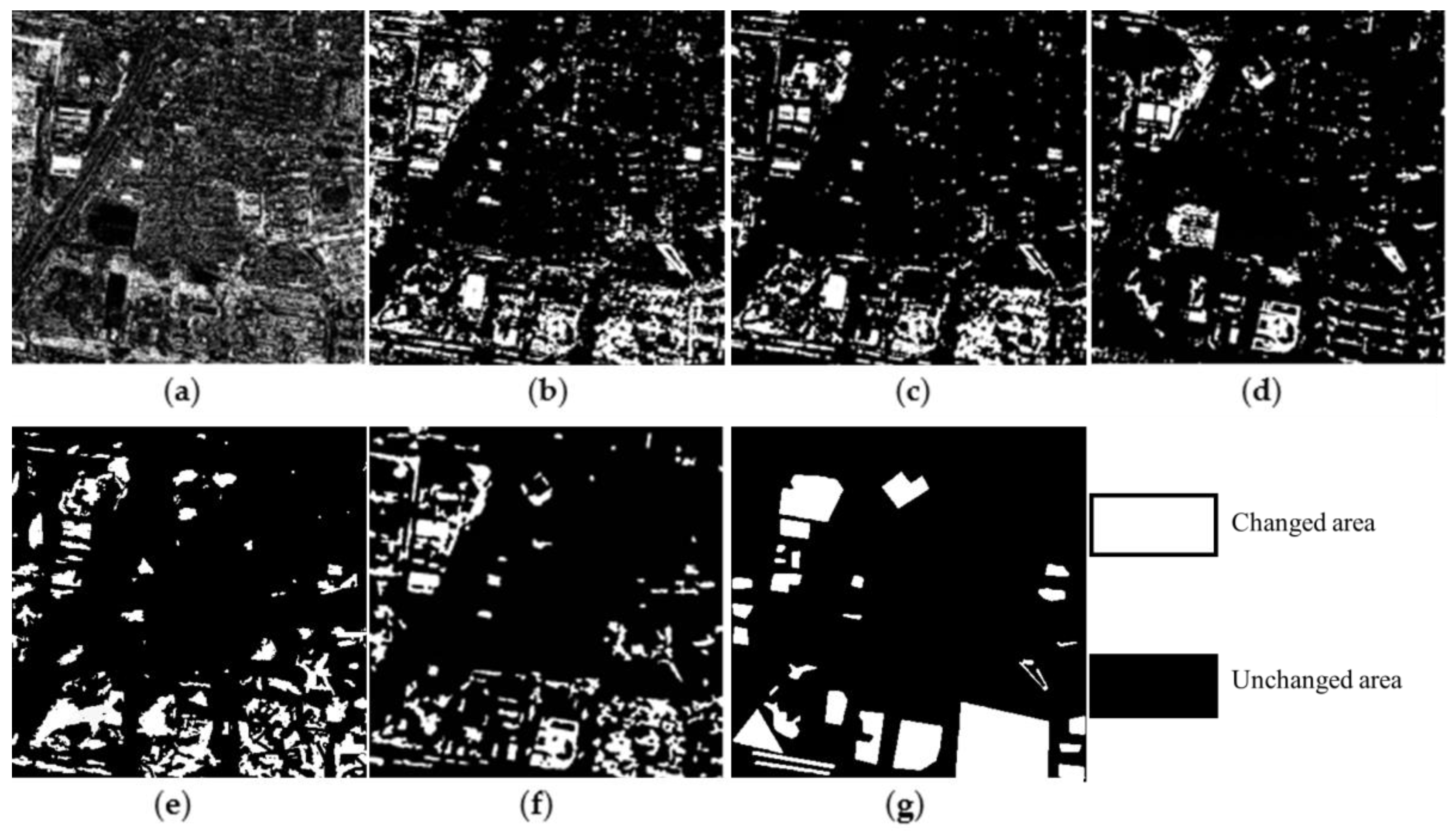
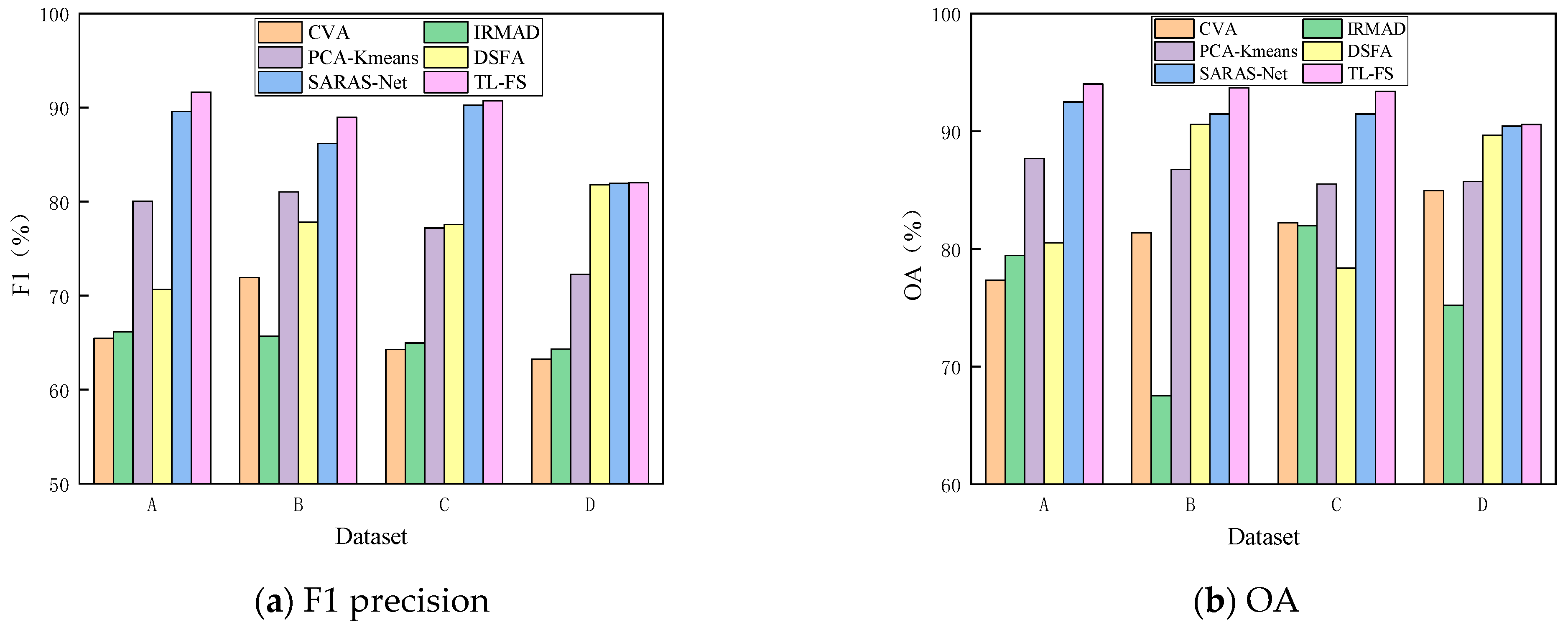
3.3. Experimental Results
4. Discussion
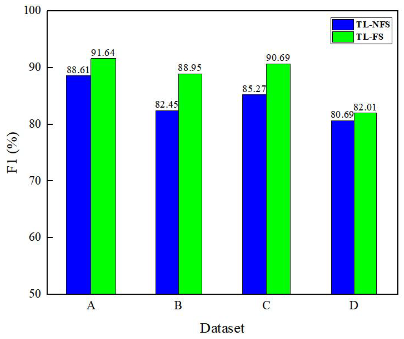
4.1. Necessity of Change Feature Selection
4.2. The Role of the Feature Variance Algorithm
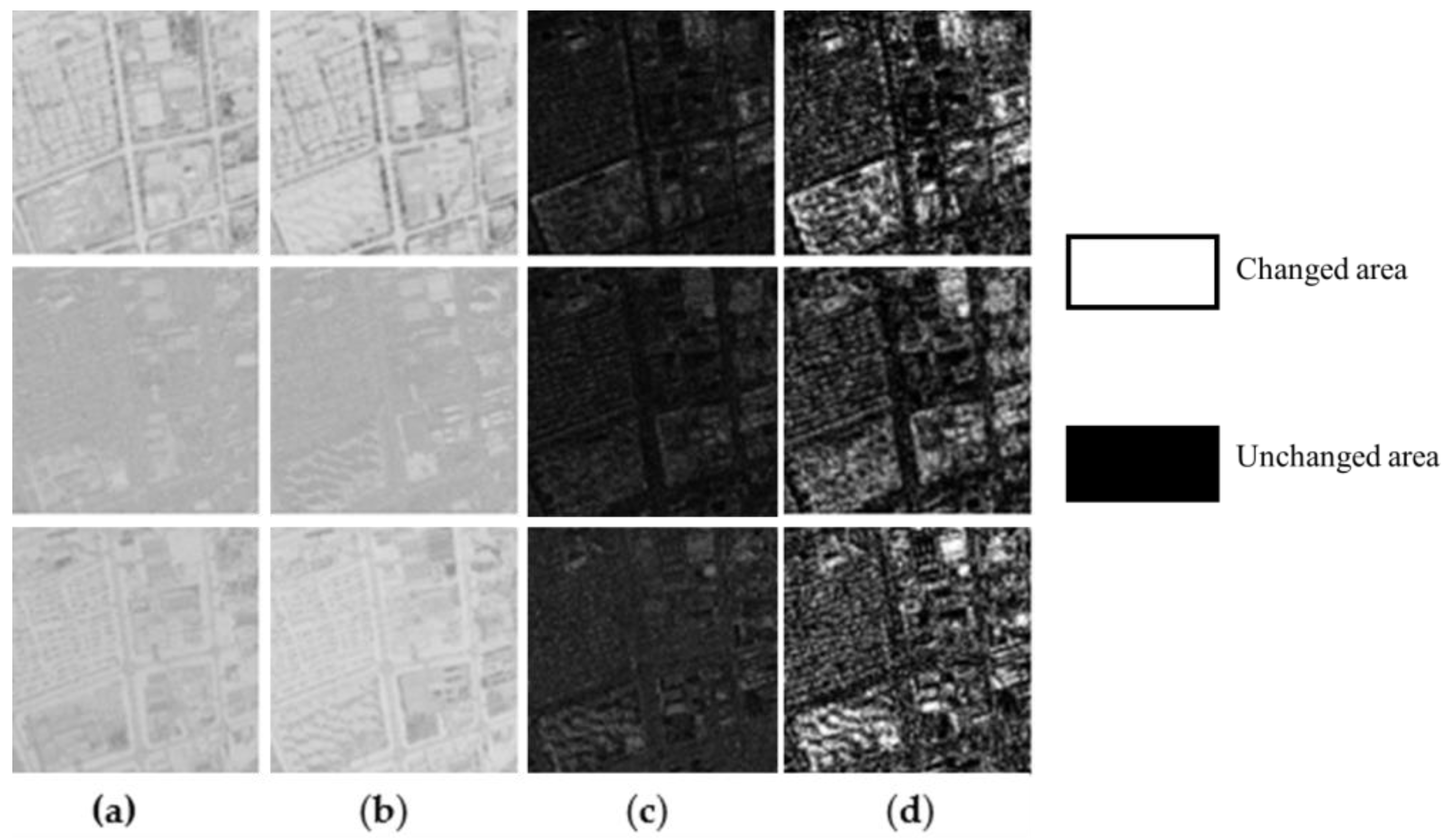
4.3. Analysis of Features Extraction Results from Different Layers
4.4. Comparison of the Results and Running Time of TL-FS Method
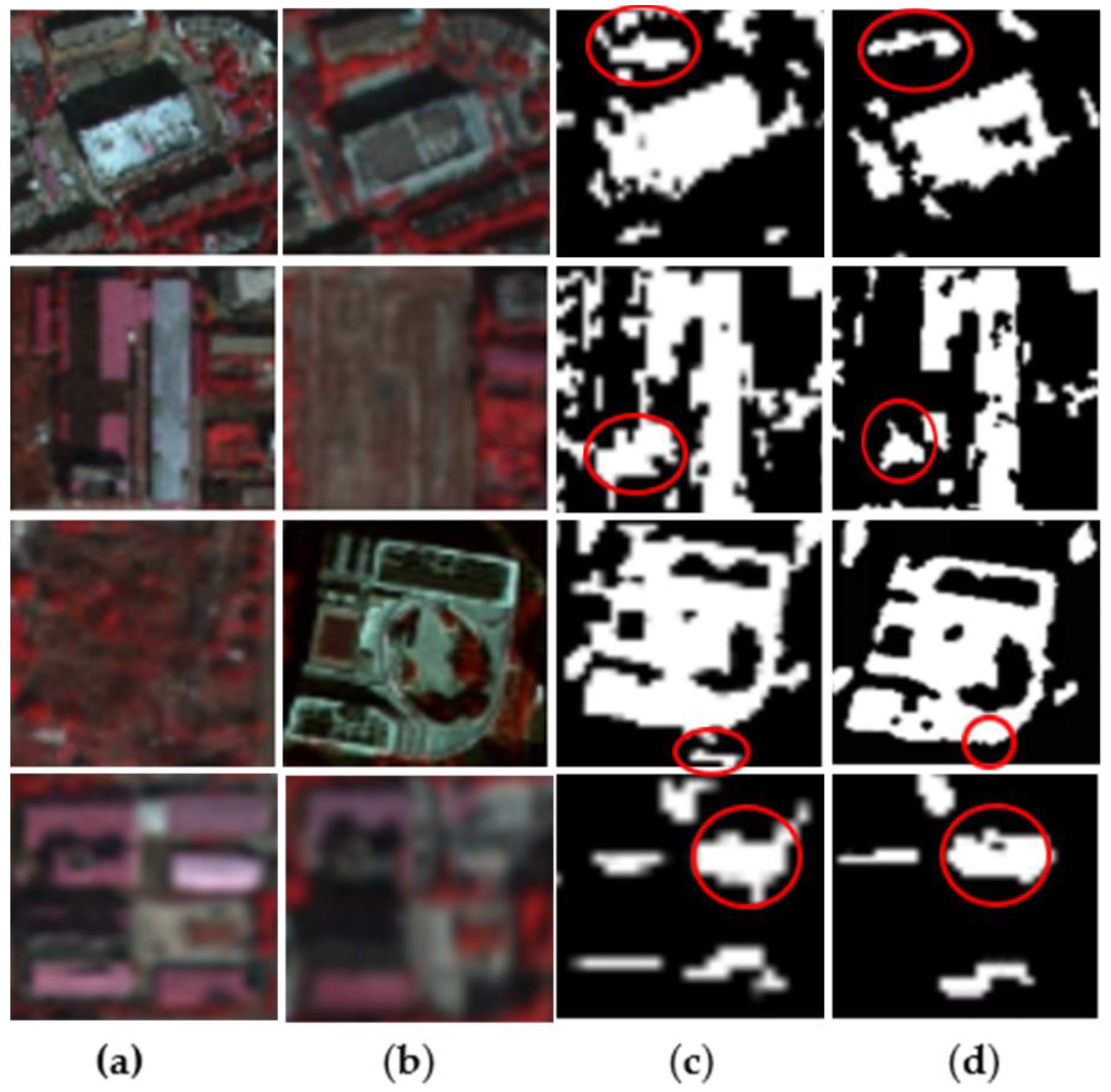
4.4.1. Discussion of Localized Test Results
4.4.2. Running Time
5. Conclusions
Author Contributions
Funding
Data Availability Statement
Acknowledgments
Conflicts of Interest
References
- Singh, A. Review article digital change detection techniques using remotely-sensed data. Int. J. Remote Sens. 1989, 10, 989–1003. [Google Scholar] [CrossRef]
- Xian, G.; Homer, C.; Fry, J. Updating the 2001 National Land Cover Database land cover classification to 2006 by using Landsat imagery change detection methods. Remote Sens. Environ. 2009, 113, 1133–1147. [Google Scholar] [CrossRef]
- Coppin, P.; Lambin, E.; Jonckheere, I.; Muys, B. Digital change detection methods in natural ecosystem monitoring: A review. J. Int. J. Remote Sens. 2004, 25, 1565–1596. [Google Scholar] [CrossRef]
- Li, H.; Xiao, G.; Xia, T.; Tang, Y.Y.; Li, L. Hyperspectral image classification using functional data analysis. IEEE Trans. Cybern. 2013, 44, 1544–1555. [Google Scholar]
- Lu, X.; Yuan, Y.; Zheng, X. Joint dictionary learning for multispectral change detection. IEEE Trans. Cybern. 2016, 47, 884–897. [Google Scholar] [CrossRef] [PubMed]
- Wen, D.; Huang, X.; Bovolo, F.; Li, J.; Ke, X.; Zhang, A.; Benediktsson, J.A. Change detection from very-high-spatial-resolution optical remote sensing images: Methods, applications, and future directions. IEEE Geosci. Remote Sens. Mag. 2021, 9, 68–101. [Google Scholar] [CrossRef]
- Shafique, A.; Cao, G.; Khan, Z.; Asad, M.; Aslam, M. Deep learning-based change detection in remote sensing images: A review. Remote Sens. 2022, 14, 871. [Google Scholar] [CrossRef]
- Liang, S.; Yu, M.; Lu, W.; Ji, X.; Tang, X.; Liu, X.; You, R. A lightweight vision transformer with symmetric modules for vision tasks. Intell. Data Anal. 2023, 27, 1741–1757. [Google Scholar] [CrossRef]
- Asokan, A.; Anitha, J. Change detection techniques for remote sensing applications: A survey. Earth Sci. Inform. 2019, 12, 143–160. [Google Scholar] [CrossRef]
- Shi, W.; Zhang, M.; Zhang, R.; Chen, S.; Zhan, Z. Change detection based on artificial intelligence: State-of-the-art and challenges. Remote Sens. 2020, 12, 1688. [Google Scholar] [CrossRef]
- Lin, S.; Yao, X.; Liu, X.; Wang, S.; Chen, H.-M.; Ding, L.; Zhang, J.; Chen, G.; Mei, Q. MS-AGAN: Road Extraction via Multi-Scale Information Fusion and Asymmetric Generative Adversarial Networks from High-Resolution Remote Sensing Images under Complex Backgrounds. Remote Sens. 2023, 15, 3367. [Google Scholar] [CrossRef]
- Wang, L.; Li, R.; Zhang, C.; Fang, S.; Duan, C.; Meng, X.; Atkinson, P.M. UNetFormer: A UNet-like transformer for efficient semantic segmentation of remote sensing urban scene imagery. ISPRS J. Photogramm. Remote Sens. 2022, 190, 196–214. [Google Scholar] [CrossRef]
- Hussain, M.; Chen, D.; Cheng, A.; Wei, H.; Stanley, D. Change detection from remotely sensed images: From pixel-based to object-based approaches. ISPRS J. Photogramm. Remote Sens. 2013, 80, 91–106. [Google Scholar] [CrossRef]
- Malila, W.A. Change vector analysis: An approach for detecting forest changes with Landsat. In Proceedings of the LARS Symposia, West Lafayette, IN, USA, 1 January 1980; p. 385. [Google Scholar]
- Chen, J.; Lu, M.; Chen, X.; Chen, J.; Chen, L. A spectral gradient difference based approach for land cover change detection. ISPRS J. Photogramm. Remote Sens. 2013, 85, 1–12. [Google Scholar] [CrossRef]
- Fung, T.; LeDrew, E. Application of principal components analysis to change detection. Photogramm. Eng. Remote Sens. 1987, 53, 1649–1658. [Google Scholar]
- Canty, M.J.; Nielsen, A.A. Automatic radiometric normalization of multitemporal satellite imagery with the iteratively re-weighted MAD transformation. Remote Sens. Environ. 2008, 112, 1025–1036. [Google Scholar] [CrossRef]
- Chen, J.; Chen, X.; Cui, X.; Chen, J. Change vector analysis in posterior probability space: A new method for land cover change detection. IEEE Geosci. Remote Sens. Lett. 2010, 8, 317–321. [Google Scholar] [CrossRef]
- Praveen, B.; Parveen, S.; Akram, V. Urban Change Detection Analysis Using Big Data and Machine Learning: A Review. In Advancements in Urban Environmental Studies: Application of Geospatial Technology and Artificial Intelligence in Urban Studies; Rahman, A., Sen Roy, S., Talukdar, S., Shahfahad, Eds.; Springer International Publishing: Cham, Switzerland, 2023; pp. 125–133. [Google Scholar]
- Zhong, Y.; Ma, A.; soon Ong, Y.; Zhu, Z.; Zhang, L. Computational intelligence in optical remote sensing image processing. Appl. Soft Comput. 2018, 64, 75–93. [Google Scholar] [CrossRef]
- Ronneberger, O.; Fischer, P.; Brox, T. U-net: Convolutional networks for biomedical image segmentation. In Proceedings of the Medical Image Computing and Computer-Assisted Intervention–MICCAI 2015: 18th International Conference, Munich, Germany, 5–9 October 2015; Proceedings, Part III 18. 2015; pp. 234–241. [Google Scholar]
- Chen, L.-C.; Papandreou, G.; Schroff, F.; Adam, H. Rethinking Atrous Convolution for Semantic Image Segmentation. arXiv 2017, arXiv:1706.05587. [Google Scholar]
- Szegedy, C.; Liu, W.; Jia, Y.; Sermanet, P.; Reed, S.; Anguelov, D.; Erhan, D.; Vanhoucke, V.; Rabinovich, A. Going deeper with convolutions. In Proceedings of the IEEE Conference on Computer Vision and Pattern Recognition, Boston, MA, USA, 7–12 June 2015; pp. 1–9. [Google Scholar]
- LeCun, Y. LeNet-5, Convolutional Neural Networks. 2015. Available online: http://yann.lecun.com/exdb/lenet (accessed on 20 August 2023).
- Zahangir Alom, M.; Taha, T.M.; Yakopcic, C.; Westberg, S.; Sidike, P.; Shamima Nasrin, M.; Van Esesn, B.C.; Awwal, A.A.S.; Asari, V.K. The history began from alexnet: A comprehensive survey on deep learning approaches. arXiv 2018, arXiv:1803.01164. [Google Scholar]
- He, K.; Zhang, X.; Ren, S.; Sun, J. Deep residual learning for image recognition. In Proceedings of the IEEE Conference on Computer Vision and Pattern Recognition, Las Vegas, NV, USA, 27–30 June 2016; pp. 770–778. [Google Scholar]
- Khelifi, L.; Mignotte, M. Deep learning for change detection in remote sensing images: Comprehensive review and meta-analysis. IEEE Access 2020, 8, 126385–126400. [Google Scholar] [CrossRef]
- Liu, J.; Chen, K.; Xu, G.; Sun, X.; Yan, M.; Diao, W.; Han, H. Convolutional neural network-based transfer learning for optical aerial images change detection. IEEE Geosci. Remote Sens. Lett. 2019, 17, 127–131. [Google Scholar] [CrossRef]
- Andresini, G.; Appice, A.; Ienco, D.; Malerba, D. SENECA: Change detection in optical imagery using Siamese networks with Active-Transfer Learning. Expert Syst. Appl. 2023, 214, 119123. [Google Scholar] [CrossRef]
- Zhan, T.; Gong, M.; Jiang, X.; Zhao, W. Transfer learning-based bilinear convolutional networks for unsupervised change detection. IEEE Geosci. Remote Sens. Lett. 2021, 19, 8010405. [Google Scholar] [CrossRef]
- Habibollahi, R.; Seydi, S.T.; Hasanlou, M.; Mahdianpari, M. TCD-Net: A novel deep learning framework for fully polarimetric change detection using transfer learning. Remote Sens. 2022, 14, 438. [Google Scholar] [CrossRef]
- Song, A.; Choi, J. Fully convolutional networks with multiscale 3D filters and transfer learning for change detection in high spatial resolution satellite images. Remote Sens. 2020, 12, 799. [Google Scholar] [CrossRef]
- Li, N.; Wu, J. Remote sensing image detection based on feature enhancement SSD. In Proceedings of the 2023 35th Chinese Control and Decision Conference (CCDC), Yichang, China, 20–22 May 2023; pp. 460–465. [Google Scholar]
- Simonyan, K.; Zisserman, A. Very Deep Convolutional Networks for Large-Scale Image Recognition. arXiv 2014, arXiv:1409.1556. [Google Scholar]
- He, X.; Ji, M.; Zhang, C.; Bao, H. A variance minimization criterion to feature selection using laplacian regularization. IEEE Trans. Pattern Anal. Mach. Intell. 2011, 33, 2013–2025. [Google Scholar]
- He, X.; Cai, D.; Niyogi, P. Laplacian score for feature selection. In Proceedings of the 18th International Conference on Neural Information Processing Systems, Vancouver, BC, Canada, 5–8 December 2005; pp. 507–514. [Google Scholar]
- Bezdek, J.C.; Ehrlich, R.; Full, W. FCM: The fuzzy c-means clustering algorithm. Comput. Geosci. 1984, 10, 191–203. [Google Scholar] [CrossRef]
- Li, X.; Zhang, Y.; Cui, Q.; Yi, X.; Zhang, Y. Tooth-marked tongue recognition using multiple instance learning and CNN features. IEEE Trans. Cybern. 2018, 49, 380–387. [Google Scholar] [CrossRef]
- LeCun, Y.; Bengio, Y.; Hinton, G. Deep learning. Nature 2015, 521, 436–444. [Google Scholar] [CrossRef] [PubMed]
- Hou, B.; Wang, Y.; Liu, Q. Change detection based on deep features and low rank. IEEE Geosci. Remote Sens. Lett. 2017, 14, 2418–2422. [Google Scholar] [CrossRef]
- Xia, G.-S.; Hu, J.; Hu, F.; Shi, B.; Bai, X.; Zhong, Y.; Zhang, L.; Lu, X. AID: A benchmark data set for performance evaluation of aerial scene classification. IEEE Trans. Geosci. Remote Sens. 2017, 55, 3965–3981. [Google Scholar] [CrossRef]
- Du, B.; Ru, L.; Wu, C.; Zhang, L. Unsupervised deep slow feature analysis for change detection in multi-temporal remote sensing images. IEEE Trans. Geosci. Remote Sens. 2019, 57, 9976–9992. [Google Scholar] [CrossRef]
- Chen, C.-P.; Hsieh, J.-W.; Chen, P.-Y.; Hsieh, Y.-K.; Wang, B.-S. SARAS-net: Scale and relation aware siamese network for change detection. In Proceedings of the AAAI Conference on Artificial Intelligence, Washington, DC, USA, 7–14 February 2023; pp. 14187–14195. [Google Scholar]


| Layer | Type | Filter | Kernel Size |
|---|---|---|---|
| input | X1, X2 | - | - |
| convolution | conv1, conv2 | 64 | 3 × 3/1 |
| maximum pooling | Pool1 | - | 2 × 2/2 |
| convolution | conv3, conv4 | 128 | 1 × 1/1 |
| maximum pooling | Pool2 | - | 2 × 2/2 |
| convolution | conv5, conv6, conv7 | 256 | 3 × 3/1 |
| Experimental Sequence Number | Method | Precision (%) | Recall (%) | F1 (%) | OA (%) | Running Time (s) |
|---|---|---|---|---|---|---|
| Dataset A | CVA | 55.68 | 79.47 | 65.48 | 77.32 | 1.68 |
| IRMAD | 57.25 | 78.31 | 66.14 | 79.44 | 2.37 | |
| PCA-Kmeans | 78.06 | 82.13 | 80.04 | 87.67 | 35.28 | |
| DSFA | 86.41 | 59.77 | 70.66 | 80.49 | 463.43 | |
| SARAS-Net | 90.56 | 88.64 | 89.59 | 92.49 | 124.44 | |
| TL-FS | 93.72 | 89.65 | 91.64 | 94.01 | 74.37 | |
| Dataset B | CVA | 76.17 | 68.11 | 71.91 | 81.35 | 1.36 |
| IRMAD | 67.93 | 63.57 | 65.68 | 67.51 | 1.97 | |
| PCA-Kmeans | 70.35 | 75.72 | 81.02 | 86.74 | 45.32 | |
| DSFA | 75.24 | 80.56 | 77.81 | 90.58 | 472.63 | |
| SARAS-Net | 89.72 | 82.87 | 86.18 | 91.44 | 116.51 | |
| TL-FS | 91.63 | 85.74 | 88.95 | 93.66 | 70.26 | |
| Dataset C | CVA | 65.14 | 63.45 | 64.28 | 82.22 | 2.33 |
| IRMAD | 63.27 | 66.82 | 65.00 | 81.97 | 3.61 | |
| PCA-Kmeans | 85.52 | 70.34 | 77.19 | 85.49 | 72.25 | |
| DSFA | 80.48 | 74.83 | 77.54 | 78.35 | 619.34 | |
| SARAS-Net | 91.59 | 88.94 | 90.25 | 91.44 | 160.26 | |
| TL-FS | 92.30 | 89.14 | 90.69 | 93.40 | 82.45 | |
| Dataset D | CVA | 69.53 | 59.21 | 63.24 | 84.94 | 2.12 |
| IRMAD | 67.16 | 61.75 | 64.34 | 75.21 | 2.58 | |
| PCA-Kmeans | 77.84 | 67.42 | 72.26 | 85.73 | 58.32 | |
| DSFA | 80.35 | 83.26 | 81.80 | 89.64 | 324.20 | |
| SARAS-Net | 81.74 | 82.12 | 81.93 | 90.44 | 140.21 | |
| TL-FS | 85.21 | 79.05 | 82.01 | 90.57 | 65.79 |
| Dataset | Method | Running Time (s) |
|---|---|---|
| A | TL-NFS | 113.54 |
| TL-FS | 74.37 | |
| B | TL-NFS | 101.92 |
| TL-FS | 70.26 | |
| C | TL-NFS | 126.48 |
| TL-FS | 82.45 | |
| D | TL-NFS | 94.83 |
| TL-FS | 65.79 |
Disclaimer/Publisher’s Note: The statements, opinions and data contained in all publications are solely those of the individual author(s) and contributor(s) and not of MDPI and/or the editor(s). MDPI and/or the editor(s) disclaim responsibility for any injury to people or property resulting from any ideas, methods, instructions or products referred to in the content. |
© 2024 by the authors. Licensee MDPI, Basel, Switzerland. This article is an open access article distributed under the terms and conditions of the Creative Commons Attribution (CC BY) license (https://creativecommons.org/licenses/by/4.0/).
Share and Cite
Chen, Q.; Yue, P.; Xu, Y.; Cao, S.; Zhou, L.; Liu, Y.; Luo, J. Feature-Selection-Based Unsupervised Transfer Learning for Change Detection from VHR Optical Images. Remote Sens. 2024, 16, 3507. https://doi.org/10.3390/rs16183507
Chen Q, Yue P, Xu Y, Cao S, Zhou L, Liu Y, Luo J. Feature-Selection-Based Unsupervised Transfer Learning for Change Detection from VHR Optical Images. Remote Sensing. 2024; 16(18):3507. https://doi.org/10.3390/rs16183507
Chicago/Turabian StyleChen, Qiang, Peng Yue, Yingjun Xu, Shisong Cao, Lei Zhou, Yang Liu, and Jianhui Luo. 2024. "Feature-Selection-Based Unsupervised Transfer Learning for Change Detection from VHR Optical Images" Remote Sensing 16, no. 18: 3507. https://doi.org/10.3390/rs16183507
APA StyleChen, Q., Yue, P., Xu, Y., Cao, S., Zhou, L., Liu, Y., & Luo, J. (2024). Feature-Selection-Based Unsupervised Transfer Learning for Change Detection from VHR Optical Images. Remote Sensing, 16(18), 3507. https://doi.org/10.3390/rs16183507