Two-Dimensional Direction Finding for L-Shaped Coprime Array via Minimization of the Ratio of the Nuclear Norm and the Frobenius Norm

Abstract

More recently, the ability of the coprime array to yield large array apertures and high degrees of freedom in comparison with the uniform linear array (ULA) has drawn an enormous amount of attention. In light of this, we propose a low-rank matrix completion algorithm via minimization of the ratio of the nuclear norm and the Frobenius norm (N/F) to solve the two-dimensional (2D) direction finding problem for the L-shaped coprime array (LsCA). Specifically, we first interpolate the virtual co-array signal related to the cross-correlation matrix (CCM) and utilize the interpolated virtual signal for Toeplitz matrix reconstruction. Then, the N/F method is employed to perform low-rank matrix completion on the reconstructed matrix. Finally, exploiting the conjugate symmetry characteristics of the completed matrix, we further develop a direction-finding algorithm that enables 2D angle estimation. Remarkably, the 2D angles are able to be automatically paired by the proposed algorithm. Numerical simulation findings demonstrate that the proposed N/F algorithm generates excellent angular resolution and computational complexity. Furthermore, this algorithm yields better estimation accuracy compared to the competing algorithms.

1. Introduction

Direction finding has been a popular subject in array signal processing, which has received an enormous amount of interest in applications including navigation, sonar, and radar [1,2,3,4,5,6,7,8,9,10]. Practically, two-dimensional (2D) direction finding is more in line with the requirements of practical applications than one-dimensional (1D) direction finding. In recent decades, 2D array structures, including the parallel-shaped array (PsA) [11,12,13], L-shaped array (LsA) [14,15,16,17,18,19,20,21,22,23,24,25,26], uniform circular array (UCA) [27,28,29,30,31,32], and uniform rectangular array (URA) [33,34,35,36,37,38], have been employed in 2D direction finding algorithms. In addition, since the LsA has a simple structure and easy implementation, the 2D direction finding for the LsA is the most popular research topic.

To enable the 2D direction finding for the LsA, various methods have been proposed. In [17], a generalized propagator method (PM) that only needs matrix linear operations is proposed. Gu et al. [18] proposed a joint SVD (JSVD) to enhance the 2D direction finding performance by utilizing the cross-correlation matrix (CCM) that has no noise term. In [19], an effective array aperture extension technique (EAET) is proposed by taking into account the conjugate symmetry characteristic of the CCM, which in turn enhances the estimation performance. To simultaneously enlarge the array apertures and virtual snapshots, Dong et al. [20] constructed a large array-received-data-like matrix, taking into account the conjugate symmetry characteristic of the CCM. To extend the number of resolvable source signals, generalized conjugate symmetry is utilized in [21] to further enlarge the array aperture and virtual snapshots, followed by building a QCCQP problem to boost the direction finding accuracy. In [22], an iterative tensor-based 2D angle estimation is developed, which can effectively remove the cross-term associated with the noise term. Jin et al. [23] investigate an LsA-based localization method for achieving underdetermined 2D angle estimation of incoherently distributed sources, which generates high-accuracy estimation performance in the absence of any prior information regarding the angular distribution. However, the majority of the above methods are only applicable to the LsA, whose subarrays are uniform linear arrays (ULAs), thereby not directly utilizing the advantage of large virtual difference co-arrays of sparse arrays.

This paper proposes a 2D direction finding algorithm via minimization of the ratio of the nuclear norm and the Frobenius norm (N/F) for the L-shaped coprime array (LsCA), motivated by the larger array apertures and higher degrees of freedom of the LsCA. This algorithm first interpolates the virtual co-array signal corresponding to the CCM and performs a Toeplitz matrix reconstruction. Then, the N/F method is utilized to perform low-rank matrix completion on the reconstructed matrix. Finally, the decoupled estimation of the 2D angles is achieved by exploiting the conjugate symmetry characteristics of the completed matrix. Numerical simulation findings illustrate that the proposed N/F algorithm generates superior performance both with regard to estimation accuracy, angular resolution, and computational complexity.

This paper’s major contributions are summarized below:

(1)

We derive the virtual co-array signal model corresponding to the CCM of LsCA and perform Toeplitz matrix reconstruction utilizing the interpolated virtual co-array signal.

(2)

Considering the zero regions of the reconstructed Toeplitz matrix, we utilize the N/F method for low-rank matrix completion. Taking into account the conjugate symmetry characteristics of the completed matrix, a direction-finding algorithm that enables 2D angle estimation is developed.

(3)

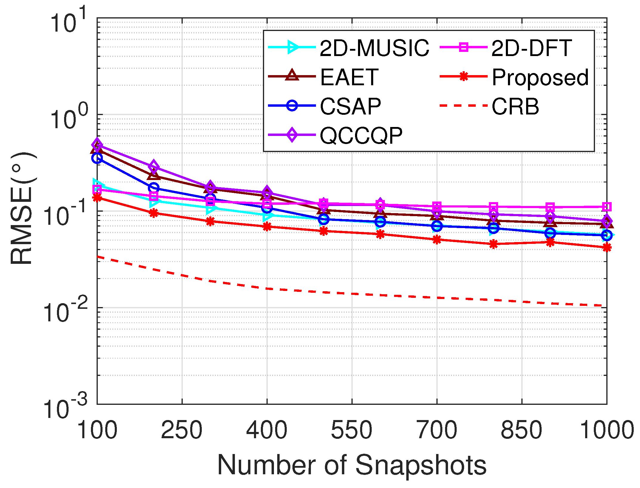
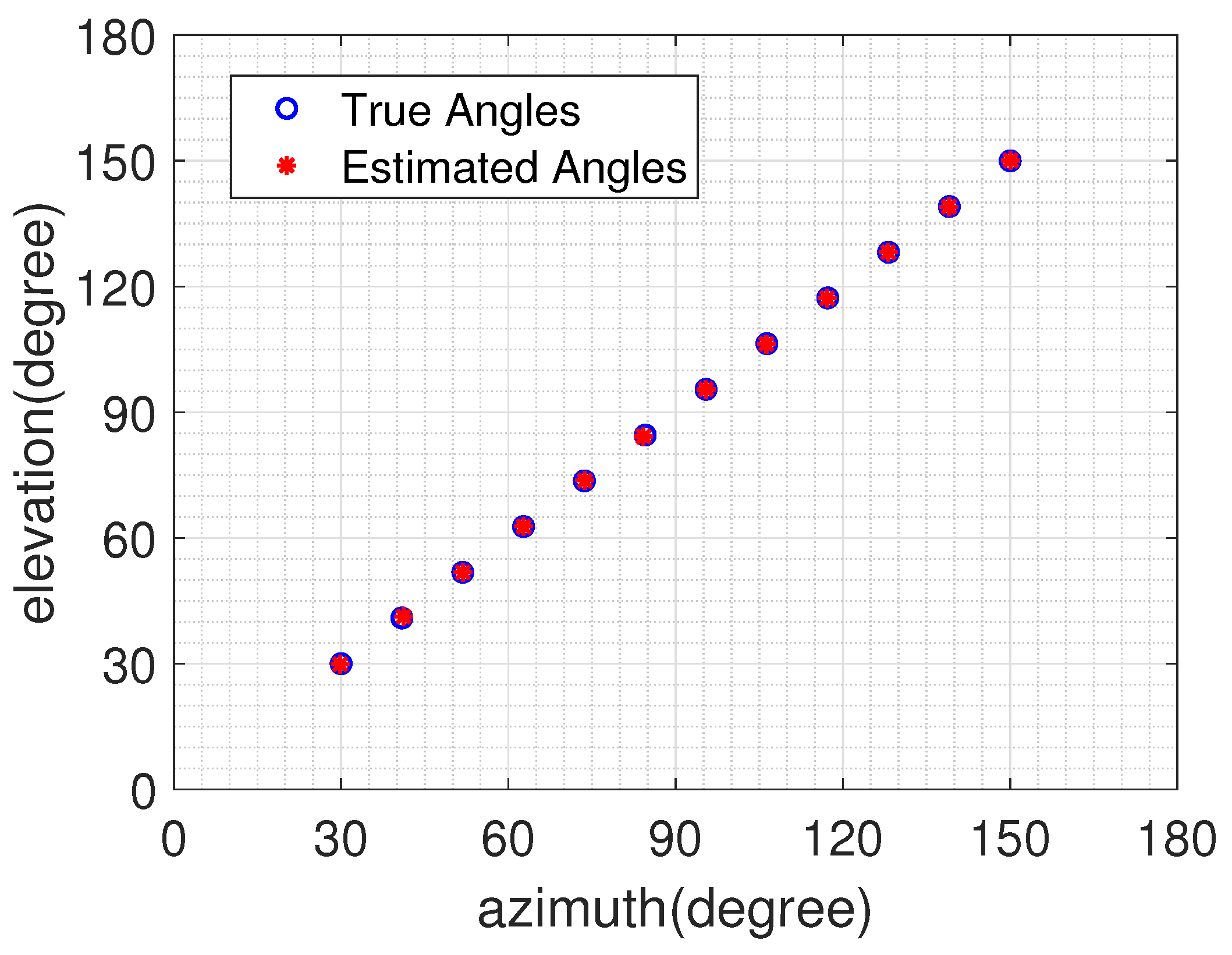
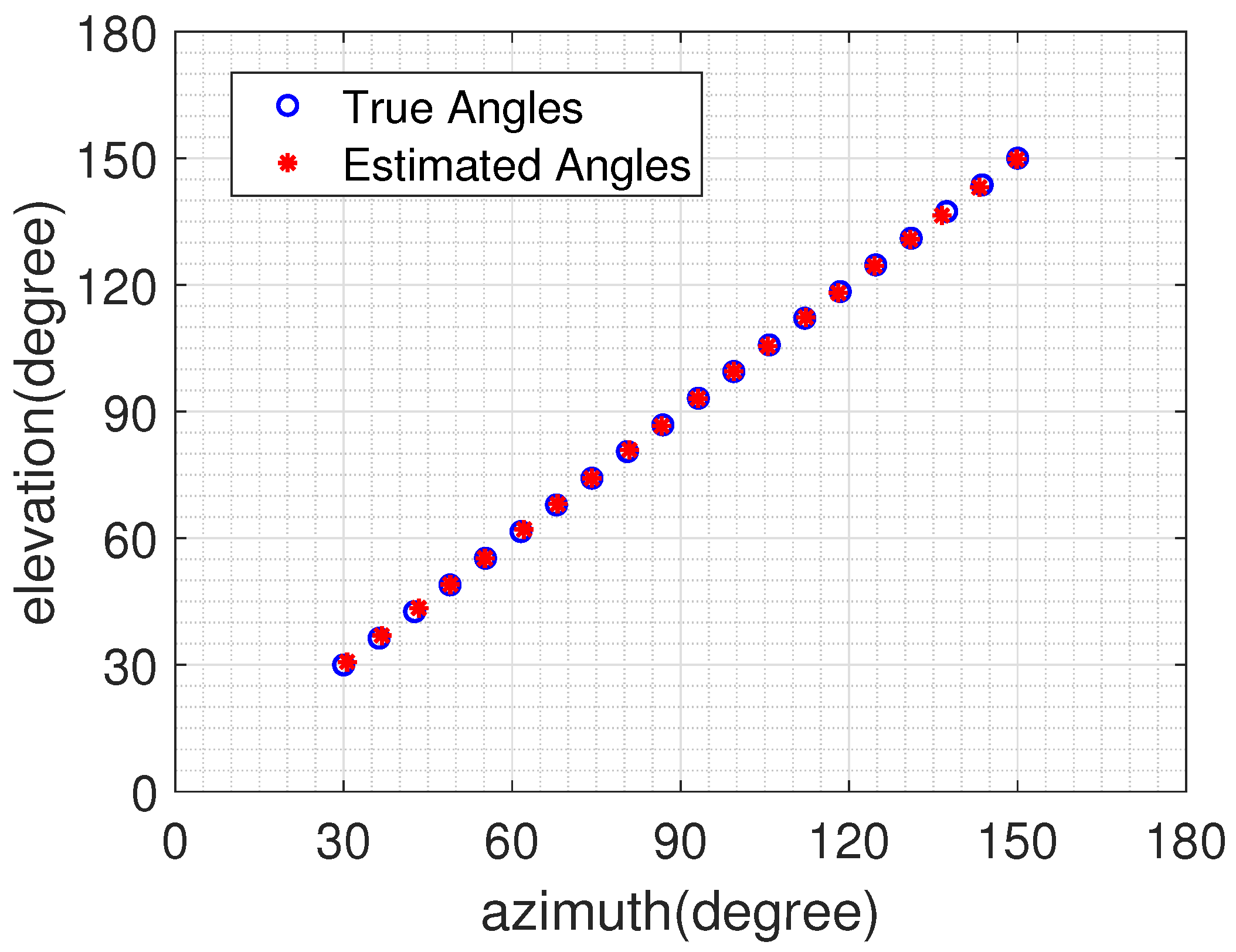
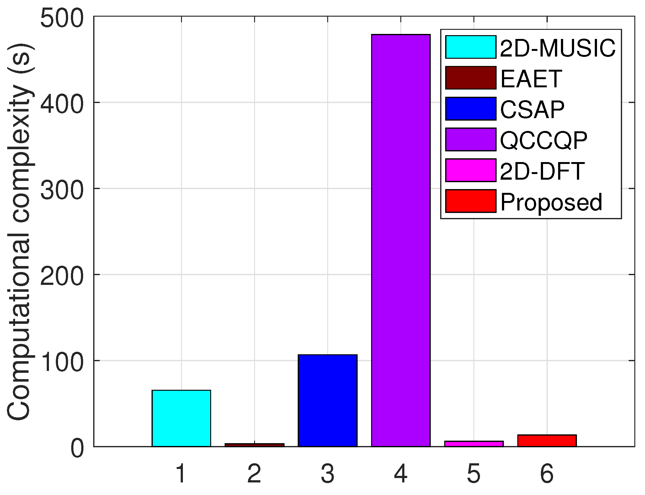
It can be observed from numerical simulation findings that the proposed N/F algorithm generates excellent performance with respect to angular resolution and computational complexity. In addition, this algorithm yields superior estimation accuracy in comparison with the competing algorithms.

The remaining sections herein are outlined below: Section 2 describes the LsCA signal model in preparation for the subsequent direction finding. In Section 3, we propose a 2D direction finding algorithm for the LsCA based on the N/F approach. Section 4 gives numerical simulations to discuss the proposed algorithm’s performance with respect to estimation accuracy, angular resolution, and computational complexity. Finally, the conclusion is presented in Section 5.

Notations: The explanations of the symbols mentioned all over the paper are given in

Table 1. Symbols and associated explanations.

Symbol	Explanation
a, $\mathbf{a}$, $\mathbf{A}$	Scalars, vectors, matrices
${\mathbf{I}}_n$, ${\mathbf{0}}_{p\times q}$, ${\mathbf{J}}_n$	n-dimensional identity matrix, $p\times q$ zero matrix, n-dimensional permutation matrix with 1 on the antidiagonal and 0 elsewhere
${(·)}^{*}$, ${(·)}^T$, ${(·)}^H$	Conjugate, transpose, Hermitian transpose
$diag(·)$	Diagonalization: Convert vectors into diagonal matrices
$arg(·)$	The phase of the argument
$E[·]$	Mathematical expectation
$vec(·)$, $\mathcal{T}(·)$	Vectorization: Convert matrices into column vectors, Toeplitz matrix operator
${∥·∥}_F$	Frobenius norm
${∥·∥}_{*}$	Nuclear norm
${\mathbb{A}}^{\left(i\right)}$	The i-th element of the set $\mathbb{A}$
$\left|\mathbb{A}\right|$	Cardinality of set $\mathbb{A}$
${\mathbf{A}}^{-1}$, ${\mathbf{A}}^{†}$, $Tr\left(\mathbf{A}\right)$	Inverse of matrix $\mathbf{A}$, pseudo-inverse of matrix $\mathbf{A}$, trace of matrix $\mathbf{A}$
⊗, ⊙	Kronecker product, Khatri-Rao product
${\left[\mathbf{A}\right]}_{i,j}$, ${\left[\mathbf{a}\right]}_i$	The $(i,j)$-th element of the matrix $\mathbf{A}$, the ith element of the vector $\mathbf{a}$
$〈a_1,a_2〉$	Integer set $\left\{a\in \mathbb{Z}\left|a_1\le a\le a_2\right.\right\}$

.

2. L-Shaped Coprime Array Signal Model

As illustrated in Figure 1, the LsCA located in the $x-z$ plane is composed of two coprime arrays ${\mathbb{S}}_i,i=x,z$ placed orthogonally along the x and z axes, respectively. Every coprime array ${\mathbb{S}}_i$ has $\left|{\mathbb{S}}_i\right|=2M_i+N_i-1$ physical sensors, consisting of two sparse ULAs [39]. Note that $M_i$ and $N_i$ are coprime integers, and the two sparse ULAs contain $2M_i$ and $N_i$ physical sensors with corresponding spacings of $N_{i}d$ and $M_{i}d$, respectively, where $d={\displaystyle \frac{\lambda }{2}}$ and $\lambda$ represents the carrier wavelength. Therefore, the sensor positions of each coprime array ${\mathbb{S}}_i$ can be denoted as ${\mathbb{S}}_{i}d$, where ${\mathbb{S}}_i=\left\{{\mathbb{S}}_i^{\left(l\right)},l\in 〈1,\left|{\mathbb{S}}_i\right|〉\right\}=\{1,N_i+1,2N_i+1,\cdots ,(2M_i-1)N_i+1,M_i+1,2M_i+1,\cdots ,(N_i-1)M_i+1\}$.

Assume that Q uncorrelated far-field narrowband source signals from directions $\{({\theta }_q,{\phi }_q),q\in 〈1,Q〉\}$ are incident on the LsCA, where ${\theta }_q\in [0,\pi ]$ and ${\phi }_q\in [0,\pi ]$ represent the azimuth and elevation angles of the qth source signal, respectively. Let $\mathbf{x}\left(t\right)$ and $\mathbf{z}\left(t\right)$ denote the data vectors received at the time t by the coprime array ${\mathbb{S}}_x$ and the coprime array ${\mathbb{S}}_z$, respectively, which are represented as

$$\mathbf{x}\left(t\right)={\mathbf{A}}_{\mathbf{x}}\mathbf{s}\left(t\right)+{\mathbf{n}}_{\mathbf{x}}\left(t\right),$$

(1)

$$\mathbf{z}\left(t\right)={\mathbf{A}}_{\mathbf{z}}\mathbf{s}\left(t\right)+{\mathbf{n}}_{\mathbf{z}}\left(t\right),$$

(2)

where $\mathbf{s}\left(t\right)$ indicates the source signal vector. ${\mathbf{A}}_{\mathbf{x}}$ and ${\mathbf{A}}_{\mathbf{z}}$ are the array manifold matrices related to the ${\mathbb{S}}_x$ and the ${\mathbb{S}}_z$, which are given as follows:

$${\mathbf{A}}_{\mathbf{x}}=\left[{\mathbf{a}}_{\mathbf{x}}\left({\theta }_1\right),{\mathbf{a}}_{\mathbf{x}}\left({\theta }_2\right),\cdots ,{\mathbf{a}}_{\mathbf{x}}\left({\theta }_Q\right)\right],$$

(3)

$${\mathbf{a}}_{\mathbf{x}}\left({\theta }_q\right)={\left[e^{-j\pi {\mathbb{S}}_x^{\left(1\right)}cos{\theta }_q},\cdots ,e^{-j\pi {\mathbb{S}}_x^{\left(\left|{\mathbb{S}}_x\right|\right)}cos{\theta }_q}\right]}^T,$$

(4)

$${\mathbf{A}}_{\mathbf{z}}=\left[{\mathbf{a}}_{\mathbf{z}}\left({\phi }_1\right),{\mathbf{a}}_{\mathbf{z}}\left({\phi }_2\right),\cdots ,{\mathbf{a}}_{\mathbf{z}}\left({\phi }_Q\right)\right],$$

(5)

$${\mathbf{a}}_{\mathbf{z}}\left({\phi }_q\right)={\left[e^{-j\pi {\mathbb{S}}_z^{\left(1\right)}cos{\phi }_q},\cdots ,e^{-j\pi {\mathbb{S}}_z^{\left(\left|{\mathbb{S}}_z\right|\right)}cos{\phi }_q}\right]}^T.$$

(6)

Furthermore, ${\mathbf{n}}_{\mathbf{x}}\left(t\right)$ and ${\mathbf{n}}_{\mathbf{z}}\left(t\right)$ are additive Gaussian white noises satisfying $\mathcal{CN}\left(\mathbf{0},{\sigma }_n^2\mathbf{I}\right)$, which are independent.

Next, the CCM of the LsCA can be presented as

$$\begin{array}{cc}\hfill {\mathbf{R}}_{\mathbf{xz}}& =E\left[\mathbf{x}\left(t\right){\mathbf{z}}^H\left(t\right)\right]\hfill \\ & ={\mathbf{A}}_{\mathbf{x}}{\mathbf{R}}_{\mathbf{ss}}{\mathbf{A}}_{\mathbf{z}}^H,\hfill \end{array}$$

(7)

where ${\mathbf{R}}_{\mathbf{ss}}=E\left[\mathbf{s}\left(t\right){\mathbf{s}}^H\left(t\right)\right]=diag\left(\mathbf{p}\right)$, and $\mathbf{p}={[{\sigma }_1^2,{\sigma }_2^2,\cdots ,{\sigma }_Q^2]}^T$ is the source signal power vector.

Vectorizing ${\mathbf{R}}_{\mathbf{xz}}$, the following virtual co-array signal is obtained:

$$\begin{array}{cc}\hfill \mathbf{y}& =vec\left({\mathbf{R}}_{\mathbf{xz}}\right)\hfill \\ & =({\mathbf{A}}_{\mathbf{z}}^{*}\otimes {\mathbf{A}}_{\mathbf{x}})vec\left({\mathbf{R}}_{\mathbf{ss}}\right)\hfill \\ & =({\mathbf{A}}_{\mathbf{z}}^{*}\odot {\mathbf{A}}_{\mathbf{x}})\mathbf{p}\hfill \\ & =\mathbf{B}\mathbf{p}.\hfill \end{array}$$

(8)

Then, eliminating the duplicate rows in $\mathbf{y}$ and sorting the rows, we obtain

$$\overline{\mathbf{y}}=\overline{\mathbf{B}}\mathbf{p},$$

(9)

where $\overline{\mathbf{B}}=[\overline{\mathbf{b}}({\theta }_1,{\phi }_1),\overline{\mathbf{b}}({\theta }_2,{\phi }_2),\cdots ,\overline{\mathbf{b}}({\theta }_Q,{\phi }_Q)]$ is the virtual array manifold matrix. Here, the vector $\overline{\mathbf{b}}({\theta }_q,{\phi }_q)$ can be represented as

$$\overline{\mathbf{b}}({\theta }_q,{\phi }_q)={\overline{\mathbf{b}}}_{\mathbf{z}}^{*}\left({\phi }_q\right)\otimes {\overline{\mathbf{b}}}_{\mathbf{x}}\left({\theta }_q\right),$$

(10)

$${\overline{\mathbf{b}}}_{\mathbf{x}}\left({\theta }_q\right)={\left[e^{-j\pi {\mathbb{D}}_x^{\left(1\right)}cos{\theta }_q},\cdots ,e^{-j\pi {\mathbb{D}}_x^{\left(\left|{\mathbb{D}}_x\right|\right)}cos{\theta }_q}\right]}^T,$$

(11)

$${\overline{\mathbf{b}}}_{\mathbf{z}}\left({\phi }_q\right)={\left[e^{-j\pi {\mathbb{D}}_z^{\left(1\right)}cos{\phi }_q},\cdots ,e^{-j\pi {\mathbb{D}}_z^{\left(\left|{\mathbb{D}}_z\right|\right)}cos{\phi }_q}\right]}^T,$$

(12)

where ${\mathbb{D}}_x={\mathbb{D}}_z$. Furthermore, ${\mathbb{D}}_x$ and ${\mathbb{D}}_z$ represent the difference co-array of ${\mathbb{S}}_x$ and ${\mathbb{S}}_z$, respectively.

3. The Proposed Algorithm

This section first utilizes the N/F method to implement the Toeplitz matrix completion associated with the virtual co-array signal $\overline{\mathbf{y}}$. Then, exploiting the conjugate symmetry characteristics of the completed matrix, the estimated 2D angles are obtained.

3.1. Low-Rank Matrix Completion

According to [39], one can deduce that ${\mathbb{D}}_x$ and ${\mathbb{D}}_z$ are not hole-free. Then, to enable the virtual co-array corresponding to the co-array signal $\overline{\mathbf{y}}$ to be consecutive, we perform the interpolation as follows:

$${\mathbb{D}}_{\mathcal{I}}=min\left({\mathbb{D}}_x\right):1:max\left({\mathbb{D}}_x\right).$$

(13)

These holes can be identified as missing sensors, with their associated virtual signals set to zero. Consequently, the interpolated signal ${\widehat{\mathbf{y}}}_{\mathcal{I}}$ is calculated as

$${\left[{\widehat{\mathbf{y}}}_{\mathcal{I}}\right]}_i=\left\{\begin{array}{c}{\left[\overline{\mathbf{y}}\right]}_i\hfill \\ 0\hfill \end{array}\right.\begin{array}{c},i\in {\mathbb{D}}_x\hfill \\ ,i\in {\mathbb{D}}_{\mathcal{I}}-{\mathbb{D}}_x\hfill \end{array},$$

(14)

Based on the interpolated signal ${\widehat{\mathbf{y}}}_{\mathcal{I}}$, a Toeplitz matrix ${\tilde{\mathbf{R}}}_{\mathbf{v}}$ is constructed of the form

$${\tilde{\mathbf{R}}}_{\mathbf{v}}=\left[\begin{array}{cccc}{\left[{\widehat{\mathbf{y}}}_{\mathcal{I}}\right]}_{L_v}\hfill & {\left[{\widehat{\mathbf{y}}}_{\mathcal{I}}\right]}_{L_v-1}\hfill & \cdots \hfill & {\left[{\widehat{\mathbf{y}}}_{\mathcal{I}}\right]}_1\hfill \\ {\left[{\widehat{\mathbf{y}}}_{\mathcal{I}}\right]}_{L_v+1}\hfill & {\left[{\widehat{\mathbf{y}}}_{\mathcal{I}}\right]}_{L_v}\hfill & \cdots \hfill & {\left[{\widehat{\mathbf{y}}}_{\mathcal{I}}\right]}_2\hfill \\ ⋮\hfill & ⋮& \ddots & ⋮\\ {\left[{\widehat{\mathbf{y}}}_{\mathcal{I}}\right]}_{2L_v-1}\hfill & {\left[{\widehat{\mathbf{y}}}_{\mathcal{I}}\right]}_{2L_v-2}& \cdots & {\left[{\widehat{\mathbf{y}}}_{\mathcal{I}}\right]}_{L_v}\end{array}\right],$$

(15)

where $L_v={\displaystyle \frac{\left|{\mathbb{D}}_{\mathcal{I}}\right|+1}{2}}$.

Since ${\widehat{\mathbf{y}}}_{\mathcal{I}}$ is obtained by zero interpolation, there are zero regions in ${\tilde{\mathbf{R}}}_{\mathbf{v}}$, i.e., ${\tilde{\mathbf{R}}}_{\mathbf{v}}$ exists with missing elements. To complete ${\tilde{\mathbf{R}}}_{\mathbf{v}}$, low-rank regularization can be applied to ${\tilde{\mathbf{R}}}_{\mathbf{v}}$. Then, in light of the rank relaxation principle [40], the low-rank matrix completion can be modeled as a matrix nuclear norm minimization (NNM) optimization problem

$$\begin{array}{cc}\hfill \underset{{\widehat{\mathbf{R}}}_{\mathbf{v}}}{min}& {∥{\widehat{\mathbf{R}}}_{\mathbf{v}}∥}_{*}\hfill \\ & s.t.{\widehat{\mathbf{R}}}_{\mathbf{v}}\circ \mathbf{G}={\tilde{\mathbf{R}}}_{\mathbf{v}},\end{array}$$

(16)

where the optimized variable ${\widehat{\mathbf{R}}}_{\mathbf{v}}$ is the completed matrix. $\mathbf{G}$ is a binary matrix, with the elements in the positions related to the zero elements of ${\tilde{\mathbf{R}}}_{\mathbf{v}}$ being 0 and the remaining elements being 1. While the NNM problem is tractable, it is extremely likely to yield suboptimal performance because the nuclear norm is essentially determined by large singular values. As such, we introduce the N/F [41] as an alternative to the nuclear norm to address the problem of unbalanced penalization for all singular values that are involved in the nuclear norm. Then, Equation (16) can be reformulated as

$$\underset{{\widehat{\mathbf{R}}}_{\mathbf{v}}}{min}\lambda {\displaystyle \frac{{∥{\widehat{\mathbf{R}}}_{\mathbf{v}}∥}_{*}}{{∥{\widehat{\mathbf{R}}}_{\mathbf{v}}∥}_F}}+{\displaystyle \frac{1}{2}}{∥{\widehat{\mathbf{R}}}_{\mathbf{v}}\circ \mathbf{G}-{\tilde{\mathbf{R}}}_{\mathbf{v}}∥}_2^2,$$

(17)

where $\lambda$ represents the regularization parameter. Taking into account that ${\tilde{\mathbf{R}}}_{\mathbf{v}}$ has the Toeplitz property, Equation (17) can be further reformulated as

$$\begin{array}{cc}\hfill \underset{\mathbf{X},\mathbf{y},{\widehat{\mathbf{R}}}_{\mathbf{v}}}{min}& \lambda {\displaystyle \frac{{∥{\widehat{\mathbf{R}}}_{\mathbf{v}}∥}_{*}}{{∥{\widehat{\mathbf{R}}}_{\mathbf{v}}∥}_F}}+{\displaystyle \frac{1}{2}}{∥{\widehat{\mathbf{R}}}_{\mathbf{v}}\circ \mathbf{G}-{\tilde{\mathbf{R}}}_{\mathbf{v}}∥}_2^2+{\displaystyle \frac{\gamma }{2}}\left[Tr\left(\mathbf{X}\right)+Tr\left(\mathcal{T}\left(\mathbf{y}\right)\right)\right]\hfill \\ & s.t.\left[\begin{array}{cc}\mathcal{T}\left(\mathbf{y}\right)& {\widehat{\mathbf{R}}}_{\mathbf{v}}\\ {\widehat{\mathbf{R}}}_{\mathbf{v}}^H& \mathbf{X}\end{array}\right]⪰0,\hfill \end{array}$$

(18)

where $\gamma$ and $\mathbf{X}$ represent the regularization parameter and the regularization matrix of the free variables for preventing trivial solutions, respectively. ${\widehat{\mathbf{R}}}_{\mathbf{v}}$ and $\mathbf{y}$ represent the optimized variables that need to be solved. As the optimization Problem (18) is convex, we prefer to solve it employing ADMM [42]. First, by introducing the constraint matrices $\mathbf{W}$ and $\mathbf{U}$, the augmented Lagrangian function for Equation (18) is defined as

$$\begin{array}{cc}\hfill \mathcal{L}\left({\widehat{\mathbf{R}}}_{\mathbf{v}},\mathbf{W},\mathbf{X},\mathbf{y},\mathbf{U},\mathbf{S},\mathsf{\Lambda }\right)& =\lambda {\displaystyle \frac{{∥{\widehat{\mathbf{R}}}_{\mathbf{v}}∥}_{*}}{{∥{\widehat{\mathbf{R}}}_{\mathbf{v}}∥}_F}}+{\displaystyle \frac{1}{2}}{∥{\widehat{\mathbf{R}}}_{\mathbf{v}}\circ \mathbf{G}-{\tilde{\mathbf{R}}}_{\mathbf{v}}∥}_2^2+〈\mathbf{S},{\widehat{\mathbf{R}}}_{\mathbf{v}}-\mathbf{W}〉\hfill \\ & +{\displaystyle \frac{{\mu }_1}{2}}{∥{\widehat{\mathbf{R}}}_{\mathbf{v}}-\mathbf{W}∥}_F^2+{\displaystyle \frac{\gamma }{2}}\left[Tr\left(\mathbf{X}\right)+Tr\left(\mathcal{T}\left(\mathbf{y}\right)\right)\right]\hfill \\ & +〈\mathsf{\Lambda },\mathbf{U}-\left[\begin{array}{cc}\mathcal{T}\left(\mathbf{y}\right)& {\widehat{\mathbf{R}}}_{\mathbf{v}}\\ {\widehat{\mathbf{R}}}_{\mathbf{v}}^H& \mathbf{X}\end{array}\right]〉+{\displaystyle \frac{{\mu }_2}{2}}{∥\mathbf{U}-\left[\begin{array}{cc}\mathcal{T}\left(\mathbf{y}\right)& {\widehat{\mathbf{R}}}_{\mathbf{v}}\\ {\widehat{\mathbf{R}}}_{\mathbf{v}}^H& \mathbf{X}\end{array}\right]∥}_F^2,\hfill \end{array}$$

(19)

where ${\mu }_1$ and ${\mu }_2$ represent the penalty parameters. $\mathbf{S}$ and $\mathsf{\Lambda }$ represent the Lagrange multipliers. Based on the ADMM framework, one can obtain the solutions to (19) by iteratively updating ${\widehat{\mathbf{R}}}_{\mathbf{v}}$, $\mathbf{W}$, $\mathbf{X}$, $\mathbf{y}$, $\mathbf{U}$, $\mathbf{S}$, and $\mathsf{\Lambda }$. Specifically, the updating process is given by

$${{\widehat{\mathbf{R}}}_{\mathbf{v}}}^{(n+1)}=arg\underset{{\widehat{\mathbf{R}}}_{\mathbf{v}}}{min}\mathcal{L}\left({\widehat{\mathbf{R}}}_{\mathbf{v}},{\mathbf{W}}^{\left(n\right)},{\mathbf{X}}^{\left(n\right)},{\mathbf{y}}^{\left(n\right)},{\mathbf{U}}^{\left(n\right)},{\mathbf{S}}^{\left(n\right)},{\mathsf{\Lambda }}^{\left(n\right)}\right),$$

(20)

$${\mathbf{W}}^{(n+1)}=arg\underset{\mathbf{W}}{min}\mathcal{L}\left({{\widehat{\mathbf{R}}}_{\mathbf{v}}}^{(n+1)},\mathbf{W},{\mathbf{X}}^{\left(n\right)},{\mathbf{y}}^{\left(n\right)},{\mathbf{U}}^{\left(n\right)},{\mathbf{S}}^{\left(n\right)},{\mathsf{\Lambda }}^{\left(n\right)}\right),$$

(21)

$${\mathbf{X}}^{(n+1)}=arg\underset{\mathbf{X}}{min}\mathcal{L}\left({{\widehat{\mathbf{R}}}_{\mathbf{v}}}^{(n+1)},{\mathbf{W}}^{(n+1)},\mathbf{X},{\mathbf{y}}^{\left(n\right)},{\mathbf{U}}^{\left(n\right)},{\mathbf{S}}^{\left(n\right)},{\mathsf{\Lambda }}^{\left(n\right)}\right),$$

(22)

$${\mathbf{y}}^{(n+1)}=arg\underset{\mathbf{y}}{min}\mathcal{L}\left({{\widehat{\mathbf{R}}}_{\mathbf{v}}}^{(n+1)},{\mathbf{W}}^{(n+1)},{\mathbf{X}}^{(n+1)},\mathbf{y},{\mathbf{U}}^{\left(n\right)},{\mathbf{S}}^{\left(n\right)},{\mathsf{\Lambda }}^{\left(n\right)}\right),$$

(23)

$${\mathbf{U}}^{(n+1)}=arg\underset{\mathbf{U}}{min}\mathcal{L}\left({{\widehat{\mathbf{R}}}_{\mathbf{v}}}^{(n+1)},{\mathbf{W}}^{(n+1)},{\mathbf{X}}^{(n+1)},{\mathbf{y}}^{(n+1)},\mathbf{U},{\mathbf{S}}^{\left(n\right)},{\mathsf{\Lambda }}^{\left(n\right)}\right),$$

(24)

$${\mathbf{S}}^{(n+1)}={\mathbf{S}}^{\left(n\right)}+{\mu }_1\left(\mathbf{S},{{\widehat{\mathbf{R}}}_{\mathbf{v}}}^{(n+1)}-{\mathbf{W}}^{(n+1)}\right),$$

(25)

$${\mathsf{\Lambda }}^{(n+1)}={\mathsf{\Lambda }}^{\left(n\right)}+{\mu }_2\left({\mathbf{U}}^{(n+1)}-\left[\begin{array}{cc}\mathcal{T}\left({\mathbf{y}}^{(n+1)}\right)& {{\widehat{\mathbf{R}}}_{\mathbf{v}}}^{(n+1)}\\ {\left[{\widehat{\mathbf{R}}}_{\mathbf{v}}^{(n+1)}\right]}^H& {\mathbf{X}}^{(n+1)}\end{array}\right]\right).$$

(26)

The iteration converges if and only if the relative error of the completion matrix between two contiguous iterations is less than the convergence threshold ${\xi }_{ADMM}>0$, i.e.,

$${\displaystyle \frac{{∥{{\widehat{\mathbf{R}}}_{\mathbf{v}}}^{(n+1)}-{{\widehat{\mathbf{R}}}_{\mathbf{v}}}^{\left(n\right)}∥}_F}{{∥{{\widehat{\mathbf{R}}}_{\mathbf{v}}}^{\left(n\right)}∥}_F}}⩽{\xi }_{ADMM}.$$

(27)

3.2. Angles Estimation

The completed matrix ${\widehat{\mathbf{R}}}_{\mathbf{v}}$ is equivalent to the CCM of LsA, i.e.,

$${\widehat{\mathbf{R}}}_{\mathbf{v}}={\widehat{\mathbf{A}}}_{\mathbf{x}}{\mathbf{R}}_{\mathbf{ss}}{\widehat{\mathbf{A}}}_{\mathbf{z}}^H,$$

(28)

where ${\widehat{\mathbf{A}}}_{\mathbf{x}}=\left[{\widehat{\mathbf{a}}}_{\mathbf{x}}\left({\theta }_1\right),{\widehat{\mathbf{a}}}_{\mathbf{x}}\left({\theta }_2\right),\cdots ,{\widehat{\mathbf{a}}}_{\mathbf{x}}\left({\theta }_Q\right)\right]$, ${\widehat{\mathbf{A}}}_{\mathbf{z}}=\left[{\widehat{\mathbf{a}}}_{\mathbf{z}}\left({\phi }_1\right),{\widehat{\mathbf{a}}}_{\mathbf{z}}\left({\phi }_2\right),\cdots ,{\widehat{\mathbf{a}}}_{\mathbf{z}}\left({\phi }_Q\right)\right]$. Here, ${\widehat{\mathbf{a}}}_{\mathbf{x}}\left({\theta }_q\right)$ and ${\widehat{\mathbf{a}}}_{\mathbf{z}}\left({\phi }_q\right)$ can respectively be represented as

$${\widehat{\mathbf{a}}}_{\mathbf{x}}\left({\theta }_q\right)={\left[1,e^{-j\pi cos{\theta }_q},\cdots ,e^{-j\pi (L_v-1)cos{\theta }_q}\right]}^T,$$

(29)

$${\widehat{\mathbf{a}}}_{\mathbf{z}}\left({\phi }_q\right)={\left[1,e^{-j\pi cos{\phi }_q},\cdots ,e^{-j\pi (L_v-1)cos{\phi }_q}\right]}^T.$$

(30)

To facilitate the selection of the first and last $L_v-1$ rows of the matrix, the selection matrixs can be defined as

$${\mathsf{\Phi }}_i=\left[{\mathbf{0}}_{\left(L_v-1\right)\times \left(i-1\right)},{\mathbf{I}}_{L_v-1},{\mathbf{0}}_{\left(L_v-1\right)\times \left(2-i\right)}\right],i=1,2.$$

(31)

Based on ${\widehat{\mathbf{A}}}_{\mathbf{x}}$, the following relationship is satisfied:

$${\mathsf{\Phi }}_2{\widehat{\mathbf{A}}}_{\mathbf{x}}={\mathsf{\Phi }}_1{\widehat{\mathbf{A}}}_{\mathbf{x}}{\mathsf{\Psi }}_{\mathbf{x}},$$

(32)

where ${\mathsf{\Psi }}_{\mathbf{x}}=diag\left([e^{-j\pi cos{\theta }_1},\cdots ,e^{-j\pi cos{\theta }_Q}]\right)$. Next, applying eigenvalue decomposition to ${\widehat{\mathbf{R}}}_{\mathbf{v}}$ yields the signal subspace ${\mathbf{E}}_{\mathbf{s}}$. Because ${\mathbf{E}}_{\mathbf{s}}$ spans the column space of ${\widehat{\mathbf{A}}}_{\mathbf{x}}$, we have

$${\mathbf{E}}_{\mathbf{s}}={\widehat{\mathbf{A}}}_{\mathbf{x}}\mathbf{T}.$$

(33)

Combining Equations (32) and (33), we can derive

$${\mathsf{\Phi }}_2{\mathbf{E}}_{\mathbf{s}}={\mathsf{\Phi }}_1{\mathbf{E}}_{\mathbf{s}}\mathsf{\Theta },$$

(34)

where $\mathsf{\Theta }={\mathbf{T}}^{-1}{\mathsf{\Psi }}_{\mathbf{x}}\mathbf{T}$. Obviously, the azimuth angle information is included in the eigenvalues of $\mathsf{\Theta }$. Therefore, $\mathsf{\Theta }$ can be estimated as

$$\widehat{\mathsf{\Theta }}={\left({\mathsf{\Phi }}_1{\mathbf{E}}_{\mathbf{s}}\right)}^{†}\left({\mathsf{\Phi }}_2{\mathbf{E}}_{\mathbf{s}}\right).$$

(35)

Let ${\omega }_q$ be the qth eigenvalue of $\widehat{\mathsf{\Theta }}$, then the azimuth angles can be estimated as

$${\widehat{\theta }}_q={cos}^{-1}\left(-{\displaystyle \frac{arg\left({\omega }_q\right)}{\pi }}\right),q=1,2,\cdots ,Q.$$

(36)

Since ${\widehat{\mathbf{A}}}_{\mathbf{x}}$ and ${\widehat{\mathbf{A}}}_{\mathbf{z}}$ are Vandermonde matrices, they satisfy the conjugate symmetry characteristics [19,20,21], i.e.,

$${\mathbf{J}}_{L_v}{\widehat{\mathbf{A}}}_{\mathbf{x}}^{*}={\widehat{\mathbf{A}}}_{\mathbf{x}}{{\mathsf{\Psi }}_{\mathbf{x}}}^{-\left(L_v-1\right)},$$

(37)

$${\widehat{\mathbf{A}}}_{\mathbf{z}}^T{\mathbf{J}}_{L_v}={{\mathsf{\Psi }}_{\mathbf{z}}}^{\left(L_v-1\right)}{\widehat{\mathbf{A}}}_{\mathbf{z}}^H,$$

(38)

where ${\mathsf{\Psi }}_{\mathbf{z}}=diag\left([e^{-j\pi cos{\phi }_1},\cdots ,e^{-j\pi cos{\phi }_Q}]\right)$. Combining Equations (28), (37) and (38), we can derive

$$\begin{array}{cc}\hfill \mathbf{Y}& ={\mathbf{J}}_{L_v}{\widehat{\mathbf{R}}}_{\mathbf{v}}^{*}{\mathbf{J}}_{L_v}\hfill \\ & ={\widehat{\mathbf{A}}}_{\mathbf{x}}{{\mathsf{\Psi }}_{\mathbf{x}}}^{-\left(L_v-1\right)}{\mathbf{R}}_{\mathbf{ss}}{{\mathsf{\Psi }}_z}^{\left(L_v-1\right)}{\widehat{\mathbf{A}}}_z^H.\hfill \end{array}$$

(39)

Next, applying Equation (31) to $\mathbf{Y}$ yields four maximally overlapping submatrices, i.e.,

$$\begin{array}{cc}\hfill {\mathbf{Y}}_1& ={\mathsf{\Phi }}_1{\mathbf{Y}\mathsf{\Phi }}_1^T\hfill \\ & ={\widehat{\mathbf{A}}}_{\mathbf{x}1}{{\mathsf{\Psi }}_{\mathbf{x}}}^{-\left(L_v-1\right)}{\mathbf{R}}_{\mathbf{ss}}{{\mathsf{\Psi }}_z}^{\left(L_v-1\right)}{\widehat{\mathbf{A}}}_{\mathbf{z}1}^H,\hfill \end{array}$$

(40)

$$\begin{array}{cc}\hfill {\mathbf{Y}}_2& ={\mathsf{\Phi }}_1{\mathbf{Y}\mathsf{\Phi }}_2^T\hfill \\ & ={\widehat{\mathbf{A}}}_{\mathbf{x}1}{{\mathsf{\Psi }}_{\mathbf{x}}}^{-\left(L_v-1\right)}{\mathbf{R}}_{\mathbf{ss}}{{\mathsf{\Psi }}_z}^{\left(L_v-2\right)}{\widehat{\mathbf{A}}}_{\mathbf{z}1}^H,\hfill \end{array}$$

(41)

$$\begin{array}{cc}\hfill {\mathbf{Y}}_3& ={\mathsf{\Phi }}_2{\mathbf{Y}\mathsf{\Phi }}_1^T\hfill \\ & ={\widehat{\mathbf{A}}}_{\mathbf{x}1}{{\mathsf{\Psi }}_{\mathbf{x}}}^{-\left(L_v-2\right)}{\mathbf{R}}_{\mathbf{ss}}{{\mathsf{\Psi }}_z}^{\left(L_v-1\right)}{\widehat{\mathbf{A}}}_{\mathbf{z}1}^H,\hfill \end{array}$$

(42)

$$\begin{array}{cc}\hfill {\mathbf{Y}}_4& ={\mathsf{\Phi }}_2{\mathbf{Y}\mathsf{\Phi }}_2^T\hfill \\ & ={\widehat{\mathbf{A}}}_{\mathbf{x}1}{{\mathsf{\Psi }}_{\mathbf{x}}}^{-\left(L_v-2\right)}{\mathbf{R}}_{\mathbf{ss}}{{\mathsf{\Psi }}_z}^{\left(L_v-2\right)}{\widehat{\mathbf{A}}}_{\mathbf{z}1}^H,\hfill \end{array}$$

(43)

where ${\widehat{\mathbf{A}}}_{\mathbf{x}1}={\mathsf{\Phi }}_1{\widehat{\mathbf{A}}}_{\mathbf{x}}$, ${\widehat{\mathbf{A}}}_{\mathbf{z}1}={\mathsf{\Phi }}_1{\widehat{\mathbf{A}}}_{\mathbf{z}}$. To extend the virtual array apertures and snapshots, a generalized received data matrix is built of the form

$$\widehat{\mathbf{Y}}=\left[\begin{array}{cc}{\mathbf{Y}}_1\hfill & {\mathbf{Y}}_3\\ {\mathbf{Y}}_2\hfill & {\mathbf{Y}}_4\end{array}\right]={\widehat{\mathbf{A}}}_{\mathbf{ex}}(\theta ,\phi ){\widehat{\mathbf{S}}}_{\mathbf{ex}}(\theta ,\phi ),$$

(44)

where

$${\mathbf{A}}_{\mathbf{ex}}(\theta ,\phi )={\left[{\widehat{\mathbf{A}}}_{\mathbf{x}1}{{\mathsf{\Psi }}_{\mathbf{z}}}^{\left(L_v-1\right)},{\widehat{\mathbf{A}}}_{\mathbf{x}1}{{\mathsf{\Psi }}_{\mathbf{z}}}^{\left(L_v-2\right)}\right]}^T,$$

(45)

$${\mathbf{S}}_{\mathbf{ex}}(\theta ,\phi )=\left[{\mathbf{R}}_{\mathbf{ss}}{{\mathsf{\Psi }}_{\mathbf{x}}}^{-\left(L_v-1\right)}{\widehat{\mathbf{A}}}_{\mathbf{z}1}^H,{\mathbf{R}}_{\mathbf{ss}}{{\mathsf{\Psi }}_{\mathbf{x}}}^{-\left(L_v-2\right)}{\widehat{\mathbf{A}}}_{\mathbf{z}1}^H\right].$$

(46)

Taking into account the matrix $\widehat{\mathbf{Y}}$, the generalized covariance matrix is denoted as ${\mathbf{R}}_{\mathbf{ex}}=E\left[\widehat{\mathbf{Y}}{\widehat{\mathbf{Y}}}^H\right]$. Setting ${\mathbf{U}}_{\mathbf{n}}$ to be the noise subspace of ${\mathbf{R}}_{\mathbf{ex}}$, we obtain

$${\mathbf{a}}_{\mathbf{ex}}^H(\theta ,\phi ){\mathbf{U}}_{\mathbf{n}}{\mathbf{U}}_{\mathbf{n}}^H{\mathbf{a}}_{\mathbf{ex}}(\theta ,\phi )=0,$$

(47)

where ${\mathbf{a}}_{\mathbf{ex}}(\theta ,\phi )={\left[{\widehat{\mathbf{a}}}_{\mathbf{x}1}\left(\theta \right)e^{-j\pi \left(L_v-1\right)cos\phi },{\widehat{\mathbf{a}}}_{\mathbf{x}1}\left(\theta \right)e^{-j\pi \left(L_v-2\right)cos\phi }\right]}^T=\mathbf{v}\left(\phi \right)\otimes {\widehat{\mathbf{a}}}_{\mathbf{x}1}\left(\theta \right)$, $\mathbf{v}\left(\phi \right)={\left[e^{-j\pi \left(L_v-1\right)cos\phi },e^{-j\pi \left(L_v-2\right)cos\phi }\right]}^T$.

Given $\left(\mathbf{AB}\right)\otimes \left(\mathbf{CD}\right)=\left(\mathbf{A}\otimes \mathbf{C}\right)\left(\mathbf{B}\otimes \mathbf{D}\right)$, we have

$$\begin{array}{cc}\hfill {\mathbf{a}}_{\mathbf{ex}}(\theta ,\phi )& =\left({\mathbf{I}}_2\mathbf{v}\left(\phi \right)\right)\otimes \left({\widehat{\mathbf{a}}}_{\mathbf{x}1}\left(\theta \right)·1\right)\hfill \\ & =\left({\mathbf{I}}_2\otimes {\widehat{\mathbf{a}}}_{\mathbf{x}1}\left(\theta \right)\right)\mathbf{v}\left(\phi \right),\hfill \end{array}$$

(48)

Substituting Equation (48) into (47) yields

$${\mathbf{v}}^H\left(\phi \right){\mathbf{M}}_{\mathbf{v}}\left(\theta \right)\mathbf{v}\left(\phi \right)=0,$$

(49)

where

$${\mathbf{M}}_{\mathbf{v}}\left(\theta \right)={\left({\mathbf{I}}_2\otimes {\widehat{\mathbf{a}}}_{\mathbf{x}1}\left(\theta \right)\right)}^H{\mathbf{U}}_{\mathbf{n}}{\mathbf{U}}_{\mathbf{n}}^H\left({\mathbf{I}}_2\otimes {\widehat{\mathbf{a}}}_{\mathbf{x}1}\left(\theta \right)\right).$$

(50)

Considering all constraints, (49) can be modeled as an optimization problem as below:

$$\begin{array}{cc}\hfill \underset{\mathbf{v}\left(\phi \right),{\mathbf{M}}_{\mathbf{v}}\left(\theta \right)}{min}& {\mathbf{v}}^H\left(\phi \right){\mathbf{M}}_{\mathbf{v}}\left(\theta \right)\mathbf{v}\left(\phi \right)\hfill \\ & s.t.{\mathbf{v}}^H\left(\phi \right)\mathbf{v}\left(\phi \right)=2.\hfill \end{array}$$

(51)

Next, substituting Equation (36) into (51), the elevation angles can be calculated as [20]

$${\widehat{\phi }}_q={cos}^{-1}\left({\displaystyle \frac{arg\left(-\frac{{\left[e_{min}\left({\mathbf{M}}_{\mathbf{v}}\left({\widehat{\theta }}_q\right)\right)\right]}_1}{{\left[e_{min}\left({\mathbf{M}}_{\mathbf{v}}\left({\widehat{\theta }}_q\right)\right)\right]}_2}\right)}{\pi }}\right),q=1,2,\cdots ,Q,$$

(52)

where ${\left[e_{min}\left({\mathbf{M}}_{\mathbf{v}}\left({\widehat{\theta }}_q\right)\right)\right]}_1$ and ${\left[e_{min}\left({\mathbf{M}}_{\mathbf{v}}\left({\widehat{\theta }}_q\right)\right)\right]}_2$ are the first and second elements of the eigenvector corresponding to the smallest eigenvalue of ${\mathbf{M}}_{\mathbf{v}}\left({\widehat{\theta }}_q\right)$, respectively. Remarkably, the 2D angles are able to be automatically paired by the proposed algorithm.

The specific implementation of the proposed N/F algorithm is outlined as presented in Algorithm 1.

Algorithm 1 Proposed N/F algorithm for LsCA structure.

Input: The signal vectors $\mathbf{x}\left(t\right)$ and $\mathbf{z}\left(t\right)$ received by the LsCA structure, number of source signals Q. Output: Paired angles $\left({\widehat{\theta }}_q,{\widehat{\phi }}_q\right),q\in 〈1,Q〉$.   1: ${\mathbf{R}}_{\mathbf{xz}}\leftarrow E\left[\mathbf{x}\left(t\right){\mathbf{z}}^H\left(t\right)\right]$.   2: $\overline{\mathbf{y}}\leftarrow$ (8) and (9). Low-rank Matrix Completion:   3: ${\widehat{\mathbf{y}}}_{\mathcal{I}}\leftarrow$ utilize (14) for virtual interpolation.   4: ${\tilde{\mathbf{R}}}_{\mathbf{v}}\leftarrow$ Toeplitz matrix reconstruction based on the interpolated signal ${\widehat{\mathbf{y}}}_{\mathcal{I}}$.   5: The N/F optimization problem is modeled based on (18) for low-rank matrix completion.   6: $\mathcal{L}\left({\widehat{\mathbf{R}}}_{\mathbf{v}},\mathbf{W},\mathbf{X},\mathbf{y},\mathbf{U},\mathbf{S},\mathsf{\Lambda }\right)\leftarrow$ utilize (19) to obtain the augmented Lagrangian function.   7: ${\widehat{\mathbf{R}}}_{\mathbf{v}}\leftarrow$ based on the ADMM framework, ${\widehat{\mathbf{R}}}_{\mathbf{v}}$, $\mathbf{W}$, $\mathbf{X}$, $\mathbf{y}$, $\mathbf{U}$, $\mathbf{S}$, and $\mathsf{\Lambda }$ are updated utilizing (20)–(26) until the iteration converges to obtain the optimal completion matrix ${\widehat{\mathbf{R}}}_{\mathbf{v}}$. Angles estimation:   8: $\widehat{\mathsf{\Theta }}\leftarrow$ (32)–(35).   9: ${\widehat{\theta }}_q\leftarrow$ perform eigenvalue decomposition to $\widehat{\mathsf{\Theta }}$ and utilize (36) to obtain the estimated azimuth angles.  10: $\widehat{\mathbf{Y}}\leftarrow$ based on the conjugate symmetry characteristics, utilize (44) to construct the generalized received data matrix.  11: Utilize (51) to model the optimization problem for solving the estimated elevation angles.  12: ${\widehat{\phi }}_q\leftarrow$ utilize (52) to obtain the estimated elevation angles.

4. Numerical Simulations

This section gives numerical simulations for discussing the proposed N/F algorithm’s performance, both regarding estimation accuracy, angular resolution, and computational complexity. In addition, the results of the 2D-MUSIC [14], EAET [19], CSAP [20], QCCQP [21], and 2D-DFT [8] algorithms are included for comparison. For 2D-MUSIC, 2D-DFT, and proposed N/F algorithms, the LsCA structure consisting of the coprime array with 10 physical sensors as subarrays in the x-axis and z-axis, respectively, is chosen as the array structure, and ${\mathbb{S}}_x={\mathbb{S}}_z=\{1,4,6,7,10,11,13,16,21,26\}$. For EAET, CSAP, and QCCQP algorithms, the LsA structure consisting of ULAs with 20 physical sensors as subarrays in the x-axis and z-axis, respectively, is chosen as the array structure. On top of that, for the proposed N/F algorithm, the parameters $\lambda$, $\gamma$, ${\mu }_1$, ${\mu }_2$, and ${\xi }_{ADMM}$ are configured as 10, $0.01$, $0.1$, $0.1$, and ${10}^{-5}$, respectively.

4.1. Estimation Accuracy Comparison

Firstly, the estimation accuracy of the 2D direction finding is assessed by the root mean square error (RMSE), of which the definition is

$$RMSE=\sqrt{{\displaystyle \frac{1}{KQ}}\sum _{k=1}^K\sum _{q=1}^Q\left({\left({\widehat{\theta }}_q^k-{\theta }_q\right)}^2+{\left({\widehat{\phi }}_q^k-{\phi }_q\right)}^2\right)},$$

(53)

where $K=300$ represents the number of Monte Carlo trials. ${\widehat{\theta }}_q^k$ and ${\widehat{\phi }}_q^k$ represent the qth estimated azimuth and elevation angles for the kth trial, respectively.

We consider three uncorrelated source signals from directions $({\theta }_1,{\phi }_1)=({80}^{\circ },{100}^{\circ })$, $({\theta }_2,{\phi }_2)=({120}^{\circ },{80}^{\circ })$ and $({\theta }_3,{\phi }_3)=({100}^{\circ },{120}^{\circ })$ incident on the array structure. In addition, the CRB [43] curve is chosen as a reference for analyzing the estimation performance. The RMSE of the estimated 2D angles at the number of snapshots $T=500$ with respect to the SNR when the SNR has a variation range of $-10$ dB to 20 dB is presented in Figure 2. It is apparent from the figure that the estimation results of all the algorithms tend to be more precise and stable when the SNR grows. Moreover, the proposed N/F algorithm is preferable to the 2D-MUSIC, EAET, CSAP, QCCQP, and 2D-DFT algorithms throughout the region of SNR variation. Contributing to this fact is that the proposed N/F algorithm completes the reconstructed Toplitz matrix and provides more useful information. The RMSE of the estimated 2D angles at SNR $=5$ dB with respect to the T when the T ranges from 100 to 1000 is shown in Figure 3. For all algorithms, the corresponding RMSE decreases with increasing T. In addition, by comparison with the 2D-MUSIC, EAET, CSAP, QCCQP, and 2D-DFT algorithms, the proposed N/F algorithm generates the highest estimation accuracy throughout a wide region of T.

On top of that, for the purpose of discussing the proposed N/F algorithm’s estimation accuracy in the cases with a larger amount of source signals, we consider $Q=12$ and $Q=20$ uncorrelated source signals uniformly located over $[{30}^{\circ },{150}^{\circ }]$ directions impinging on the LsCA structure. In these simulations, SNR and T are configured as 0 dB and 500, respectively. From the estimation results presented in Figure 4 and Figure 5, it can be found that the proposed N/F algorithm accurately detects all source signals in the two scenarios, demonstrating that the proposed N/F algorithm still possesses excellent estimation accuracy under the condition of the greater amount of source signals.

4.2. Angular Resolution Comparison

To further evaluate the proposed N/F algorithms’ performance, we utilize resolution probability to examine the angular resolution of the various algorithms. We consider two uncorrelated source signals from directions $({\theta }_1,{\phi }_1)=({80}^{\circ },{82}^{\circ })$ and $({\theta }_2,{\phi }_2)=({82}^{\circ },{80}^{\circ })$ incident on the array structure. Here, the angular separations are $\Delta \theta =\Delta \phi =2^{\circ }$ for azimuth and elevation angles. We regard the two source signals as successfully localized if

$$\begin{array}{c}∥{\widehat{\theta }}_q-{\theta }_q∥⩽{0.5}^{\circ }\hfill \\ ∥{\widehat{\phi }}_q-{\phi }_q∥⩽{0.5}^{\circ },q=1,2\hfill \end{array}$$

(54)

holds true. This example involves 300 Monte Carlo trials.

The angular resolution probabilities for various algorithms with SNR ranging from $-10$ dB to 20 dB and $T=500$ are presented in Figure 6, from which one can observe that the proposed N/F algorithm’s angular resolution is preferable to that of the 2D-MUSIC, EAET, CSAP, QCCQP, and 2D-DFT algorithms when SNR $<5$ dB, and its resolution probability reaches 1 when the SNR equals $-4$ dB. In contrast, the resolution probabilities of the 2D-MUSIC, EAET, CSAP, QCCQP, and 2D-DFT algorithms reach 1 at SNRs of 6 dB, 6 dB, 6 dB, $-2$ dB, and 2 dB, respectively. Remarkably, the 2D-MUSIC, EAET, CSAP, and 2D-DFT algorithms are completely unsuccessful in localizing the two source signals when SNR $<-5$ dB. The angular resolution probabilities for various algorithms with T ranging from 50 to 1000 and SNR $=5$ dB are presented in Figure 7, from which one can observe that only the proposed N/F algorithm succeeds in identifying the two source signals when $T<150$ and has a resolution probability of 1 when $T=100$. In comparison, the 2D-MUSIC, EAET, CSAP, QCCQP and 2D-DFT algorithms achieve an angular resolution probability of 1 at the number of snapshots T of 500, 350, 400, 150, and 500, respectively. In summary, the proposed N/F algorithm is preferable to the 2D-MUSIC, EAET, CSAP, QCCQP, and 2D-DFT algorithms in terms of angular resolution.

4.3. Computational Complexity Comparison

We also compare the computational complexity of various algorithms. In this example, we consider three uncorrelated source signals impinging on the array structure. On top of that, SNR and T are configured as 5 dB and 500, respectively. Figure 8 presents the computational complexity of various algorithms that perform 300 Monte Carlo trials. One can observe that the QCCQP algorithm has the highest computational complexity, followed by the CSAP and 2D-MUSIC algorithms. In addition, the computational complexity of EAET, 2D-DFT, and the proposed N/F algorithms is lower and close to the same. To summarize, the proposed N/F algorithm realizes moderate computational complexity.

5. Conclusions

In this paper, a 2D direction-finding algorithm for the LsCA is proposed via the N/F method. This algorithm not only enhances the 2D direction finding performance but also has the capability to automatically pair 2D angles. Numerical simulation findings demonstrate that the proposed N/F algorithm generates superior performance regarding angular resolution and computational complexity. In addition, this algorithm yields better estimation accuracy in comparison to the existing algorithms. In future research, the N/F method should be considered and applied to matrix completion for sparse planar arrays.

References

1. Krim, H.; Viberg, M. Two decades of array signal processing research: The parametric approach. IEEE Signal Process. Mag. 1996, 13, 67–94. [Google Scholar] [CrossRef]
2. Liu, D.; Zhao, Y.; Zhang, T. Sparsity-Based Two-Dimensional DOA Estimation for Co-Prime Planar Array via Enhanced Matrix Completion. Remote Sens. 2022, 14, 4690. [Google Scholar] [CrossRef]
3. Wen, F.; Shi, J.; Zhang, Z. Joint 2D-DOD, 2D-DOA, and polarization angles estimation for bistatic EMVS-MIMO radar via PARAFAC analysis. IEEE Trans. Veh. Technol. 2019, 69, 1626–1638. [Google Scholar] [CrossRef]
4. Cheng, L.; Wu, Y.C.; Zhang, J.; Liu, L. Subspace identification for DOA estimation in massive/full-dimension MIMO systems: Bad data mitigation and automatic source enumeration. IEEE Trans. Signal Process. 2015, 63, 5897–5909. [Google Scholar] [CrossRef]
5. Wen, F.; Shi, J.; He, J.; Truong, T.K. 2D-DOD and 2D-DOA estimation using sparse L-shaped EMVS-MIMO radar. IEEE Trans. Aerosp. Electron. Syst. 2022, 59, 2077–2084. [Google Scholar] [CrossRef]
6. Zhou, L.; Ye, K.; Qi, J.; Sun, H. DOA estimation based on pseudo-noise subspace for relocating enhanced nested array. IEEE Signal Process. Lett. 2022, 29, 1858–1862. [Google Scholar] [CrossRef]
7. Zhou, L.; Qi, J.; Hong, S. Enhanced Dilated Nested Arrays with Reduced Mutual Coupling for DOA Estimation. IEEE Sens. J. 2024, 24, 615–623. [Google Scholar] [CrossRef]
8. Zhang, Q.; Li, J.; Li, Y.; Li, P. A DOA tracking method based on offset compensation using nested array. IEEE Trans. Circuits Syst. II Exp. Briefs 2021, 69, 1917–1921. [Google Scholar] [CrossRef]
9. Xu, T.; Wang, X.; Huang, M.; Lan, X.; Sun, L. Tensor-Based Reduced-Dimension MUSIC Method for Parameter Estimation in Monostatic FDA-MIMO Radar. Remote Sens. 2021, 13, 3772. [Google Scholar] [CrossRef]
10. Ge, S.; Fan, C.; Wang, J.; Huang, X. Low-complexity one-bit DOA estimation for massive ULA with a single snapshot. Remote Sens. 2022, 14, 3436. [Google Scholar] [CrossRef]
11. Li, J.; Li, Y.; Zhang, X. Two-dimensional off-grid DOA estimation using unfolded parallel coprime array. IEEE Commun. Lett. 2018, 22, 2495–2498. [Google Scholar] [CrossRef]
12. Zhang, Y.; Xu, X.; Sheikh, Y.A.; Ye, Z. A rank-reduction based 2D DOA estimation algorithm for three parallel uniform linear arrays. Signal Process. 2016, 120, 305–310. [Google Scholar] [CrossRef]
13. Chen, H.; Hou, C.; Liu, W.; Zhu, W.P.; Swamy, M. Efficient two-dimensional direction-of-arrival estimation for a mixture of circular and noncircular sources. IEEE Sens. J. 2016, 16, 2527–2536. [Google Scholar] [CrossRef]
14. Zheng, Z.; Mu, S. 2D Direction FindingWith Pair-Matching Operation for L-Shaped Nested Array. IEEE Commun. Lett. 2020, 25, 975–979. [Google Scholar] [CrossRef]
15. Tayem, N.; Kwon, H.M. L-shape 2Dimensional arrival angle estimation with propagator method. IEEE Trans. Antennas Propag. 2005, 53, 1622–1630. [Google Scholar] [CrossRef]
16. Kikuchi, S.; Tsuji, H.; Sano, A. Pair-matching method for estimating 2D angle of arrival with a cross-correlation matrix. IEEE Antennas Wirel. Propag. Lett. 2006, 5, 35–40. [Google Scholar] [CrossRef]
17. Tayem, N.; Majeed, K.; Hussain, A.A. Two-dimensional DOA estimation using cross-correlation matrix with L-shaped array. IEEE Antennas Wirel. Propag. Lett. 2015, 15, 1077–1080. [Google Scholar] [CrossRef]
18. Gu, J.F.; Wei, P. Joint SVD of two cross-correlation matrices to achieve automatic pairing in 2D angle estimation problems. IEEE Antennas Wirel. Propag. Lett. 2007, 6, 553–556. [Google Scholar] [CrossRef]
19. Dong, Y.Y.; Dong, C.x.; Xu, J.; Zhao, G.q. Computationally efficient 2D DOA estimation for L-shaped array with automatic pairing. IEEE Antennas Wirel. Propag. Lett. 2016, 15, 1669–1672. [Google Scholar] [CrossRef]
20. Dong, Y.Y.; Dong, C.x.; Liu, W.; Chen, H.; Zhao, G.q. 2D DOA estimation for L-shaped array with array aperture and snapshots extension techniques. IEEE Signal Process. Lett. 2017, 24, 495–499. [Google Scholar] [CrossRef]
21. Wu, R.; Zhang, Z. Convex optimization-based 2D DOA estimation with enhanced virtual aperture and virtual snapshots extension for L-shaped array. IEEE Trans. Veh. Technol. 2020, 69, 6473–6484. [Google Scholar] [CrossRef]
22. Xu, F.; Zheng, H.; Vorobyov, S.A. Tensor-based 2D DOA estimation for L-shaped nested array. IEEE Trans. Aerosp. Electron. Syst. 2024, 60, 604–618. [Google Scholar] [CrossRef]
23. Jin, L.; Fang, J.; Liu, W.; Yu, Z.; Xu, G.; Zhu, M.; Chen, H. Underdetermined two-dimensional angles parameters estimation for incoherent distributed sources based on an L-shaped array. IEEE Sens. J. 2024, 24, 18479–18487. [Google Scholar] [CrossRef]
24. Rao, W.; Li, D.; Zhang, J.Q. A tensor-based approach to L-shaped arrays processing with enhanced degrees of freedom. IEEE Signal Process. Lett. 2017, 25, 1–5. [Google Scholar] [CrossRef]
25. Wu, X.; Zhu, W.P. On efficient gridless methods for 2D DOA estimation with uniform and sparse L-shaped arrays. Signal Process. 2022, 191, 108351. [Google Scholar] [CrossRef]
26. Xi, N.; Liping, L. A computationally efficient subspace algorithm for 2D DOA estimation with L-shaped array. IEEE Signal Process. Lett. 2014, 21, 971–974. [Google Scholar]
27. Zhang, T.; Lu, Y.; Hui, H. Compensation for the mutual coupling effect in uniform circular arrays for 2D DOA estimations employing the maximum likelihood technique. IEEE Trans. Aerosp. Electron. Syst. 2008, 44, 1215–1221. [Google Scholar] [CrossRef]
28. Wax, M.; Sheinvald, J. Direction finding of coherent signals via spatial smoothing for uniform circular arrays. IEEE Trans. Antennas Propag. 1994, 42, 613–620. [Google Scholar] [CrossRef]
29. Mathews, C.P.; Zoltowski, M.D. Eigenstructure techniques for 2D angle estimation with uniform circular arrays. IEEE Trans. Signal Process. 1994, 42, 2395–2407. [Google Scholar] [CrossRef]
30. Ding, X.; Xu, W.; Wang, Y.; Li, Y.; Huang, Y. Wideband 2D DoA Estimation with Uniform Circular Array. IEEE Sens. J. 2024, 24, 11585–11598. [Google Scholar] [CrossRef]
31. Zhou, T.; He, Z.; Shi, Q.; Lin, C.; Zhang, S. Multisnapshot High-Resolution Gridless DOA Estimation for Uniform Circular Arrays. IEEE Signal Process. Lett. 2024, 31, 1705–1709. [Google Scholar] [CrossRef]
32. Labbaf, N.; Oskouei, H.R.D.; Abedi, M.R. Robust DoA estimation in a uniform circular array antenna with errors and unknown parameters using Deep Learning. IEEE Trans. Green Commun. Netw. 2023, 7, 2143–2152. [Google Scholar] [CrossRef]
33. Zoltowski, M.D.; Haardt, M.; Mathews, C.P. Closed-form 2D angle estimation with rectangular arrays in element space or beamspace via unitary ESPRIT. IEEE Trans. Signal Process. 1996, 44, 316–328. [Google Scholar] [CrossRef]
34. Wu, H.; Hou, C.; Chen, H.; Liu, W.; Wang, Q. Direction finding and mutual coupling estimation for uniform rectangular arrays. Signal Process. 2015, 117, 61–68. [Google Scholar] [CrossRef]
35. Shen, F.F.; Liu, Y.M.; Zhao, G.H.; Chen, X.Y.; Li, X.P. Sparsity-based off-grid DOA estimation with uniform rectangular arrays. IEEE Sens. J. 2018, 18, 3384–3390. [Google Scholar] [CrossRef]
36. Ahmed, T.; Zhang, X.; Hassan, W.U. A higher-order propagator method for 2D-DOA estimation in massive MIMO systems. IEEE Commun. Lett. 2019, 24, 543–547. [Google Scholar] [CrossRef]
37. Zhang, Z.; Wen, F.; Shi, J.; He, J.; Truong, T.K. 2D-DOA estimation for coherent signals via a polarized uniform rectangular array. IEEE Signal Process. Lett. 2023, 30, 893–897. [Google Scholar] [CrossRef]
38. Heidenreich, P.; Zoubir, A.M.; Rubsamen, M. Joint 2D DOA estimation and phase calibration for uniform rectangular arrays. IEEE Trans. Signal Process. 2012, 60, 4683–4693. [Google Scholar] [CrossRef]
39. Vaidyanathan, P.P.; Pal, P. Sparse sensing with co-prime samplers and arrays. IEEE Trans. Signal Process. 2010, 59, 573–586. [Google Scholar] [CrossRef]
40. Recht, B.; Fazel, M.; Parrilo, P.A. Guaranteed minimum-rank solutions of linear matrix equations via nuclear norm minimization. SIAM Rev. 2010, 52, 471–501. [Google Scholar] [CrossRef]
41. Gao, K.; Huang, Z.H.; Guo, L. Low-rank matrix recovery problem minimizing a new ratio of two norms approximating the rank function then using an ADMM-type solver with applications. J. Comput. Appl. Math. 2024, 438, 115564. [Google Scholar] [CrossRef]
42. Boyd, S.; Parikh, N.; Chu, E.; Peleato, B.; Eckstein, J. Distributed optimization and statistical learning via the alternating direction method of multipliers. Found. Trends Mach. Learn. 2011, 3, 1–122. [Google Scholar] [CrossRef]
43. Xia, T.; Zheng, Y.; Wan, Q.; Wang, X. Decoupled estimation of 2D angles of arrival using two parallel uniform linear arrays. IEEE Trans. Antennas Propag. 2007, 55, 2627–2632. [Google Scholar] [CrossRef]
Figure 1. The LsCA structure.
Remotesensing 16 03543 g001
Figure 2. RMSE versus SNR with T = 500 .
Remotesensing 16 03543 g002
Figure 3. RMSE versus T with SNR = 5 dB.
Remotesensing 16 03543 g003
Figure 4. The proposed N/F algorithm’s estimation accuracy with Q = 12 .
Remotesensing 16 03543 g004
Figure 5. The proposed N/F algorithm’s estimation accuracy with Q = 20 .
Remotesensing 16 03543 g005
Figure 6. Resolution probability versus SNR with T = 500 .
Remotesensing 16 03543 g006
Figure 7. Resolution probability versus T with SNR = 5 dB.
Remotesensing 16 03543 g007
Figure 8. Comparison of computational complexity among different algorithms.
Remotesensing 16 03543 g008