Abstract
In this paper, the advantages of the joint use of MHz- and GHz-frequency band impulses when employing contactless ground penetration radar (GPR) for the remote sensing of biomass, the height of the wheat canopy, and underlying soil moisture were experimentally investigated. A MHz-frequency band nanosecond impulse with a duration of 1.2 ns (average frequency of 750 MHz and spectrum bandwidth of 580 MHz, at a level of –6 dB) was emitted and received by a GPR OKO-3 equipped with an AB-900 M3 antenna unit. A GHz-frequency band sub-nanosecond impulse with a duration of 0.5 ns (average frequency of 3.2 GHz and spectral bandwidth of 1.36 GHz, at a level of −6 dB) was generated using a horn antenna and a Keysight FieldFox N9917B 18 GHz vector network analyzer. It has been shown that changes in the relative amplitudes and time delays of nanosecond impulses, reflected from a soil surface covered with wheat at a height from 0 to 87 cm and fresh above-ground biomass (AGB) from 0 to 1.5 kg/m2, do not exceed 6% and 0.09 ns, respectively. GPR nanosecond impulses reflected/scattered by the wheat canopy have not been detected. In this research, sub-nanosecond impulses reflected/scattered by the wheat canopy have been confidently identified and make it possible to measure the wheat height (fresh AGB up to 2.3 kg/m2 and height up to 104 cm) with a determination coefficient (R2) of ~0.99 and a bias of ~−7 cm, as well as fresh AGB where R2 = 0.97, with a bias = −0.09 kg/m2, and a root-mean-square error of 0.1 kg/m2. The joint use of impulses in two different MHz- and GHz-frequency bands will, in the future, make it possible to create UAV-based reflectometers for simultaneously mapping the soil moisture, height, and biomass of vegetation for precision farming systems.
1. Introduction
In the near future, the entire cycle of field agricultural work will be carried out without physical human labor, instead using machines and aircraft platforms within the framework of precision agriculture [1,2,3]. Above-ground biomass (AGB), vegetation canopy height, and soil moisture under vegetation are the most important biophysical parameters that are necessary for crop management in precision agriculture. The use of unmanned aerial vehicles (UAVs) equipped with high spatial resolution sensors over large areas appears to be the most promising cost-effective remote-sensing technology for monitoring these biophysical parameters in the robotic systems of precision agriculture [2,3]. To measure AGB and vegetation canopy height, digital RGB [3], cameras taking multispectral (hyperspectral) images from the visible to infrared spectrum ranges [4,5], light detection and ranging (LiDAR) technology [6,7], combinations of the above sensors [8,9,10,11], and ultrasonic sensors [12] have been used on UAVs. The bare soil’s moisture, due to a significant correlation with the brightness of images, can be measured in the optical range (by combining multispectral and infrared bands, the accuracy increases) [13,14,15]. It seems that in the case of dense vegetation cover, microwave methods have no equal for the UAV-based remote sensing of soil moisture [16,17,18,19,20].
Optical methods for estimating vegetation biomass are based on establishing empirical modeling relationships between AGB, measured in situ, with various vegetation indices and specific spectral bands, including the use of multiple linear (nonlinear) regression methods and machine learning [4,5,21,22]. Such empirical relationships are specific to different types of crops, with the variation of the coefficient of determination (R2) ranging from 0.3 to 0.7. The accuracy of AGB estimation increases to R2 = 0.8–0.93 [22,23,24,25], when vegetation height (or textural features) is included in these empirical models. In optical methods, the height of vegetation is determined by the photogrammetric method [4,10,24]. In the absence of bare soil as a reference surface, the height of vegetation is apparently impossible to determine since the measurement error will increase unacceptably. The use of LiDAR [6,7,25,26] for a wide variety of agriculture crops makes it possible to successfully estimate not only their height, with R2~0.7–0.88 [6,26], but also fresh AGB with R2~0.68–0.82 [6]. However, in the case of densely planted potato crops, due to the very small number of scattered points under the canopy, LiDAR 3D point cloud-based methods lead to a degradation in both estimation of height (R2 = 0.50, RMSE = 12 cm) and biomass (R2 = 0.24, RMSE = 22.1 g/m2) [6], where RMSE stands for the root-mean-square error. Note that when using LiDAR, biomass is determined from empirical relationships with the density of point clouds, scattered by the canopy, or with the canopy height [6,26]. Ultrasonic sensors have a short range, and poor repeatability of canopy height measuring; therefore, they are less widely used for monitoring crop height with UAVs.
At the same time, contactless ground penetrating radar (GPR) methods have the potential to measure not only bare soil moisture [27,28,29,30,31,32] but also the height and biomass of vegetation [33], as well as soil moisture under the canopy [34,35,36,37,38]. The significant interaction (scattering and attenuation) of GHz-frequency range impulses with plant parts allows us to propose methodologies to retrieve the biophysical parameters of the vegetation canopy. Thus, in Ref. [33], empirical linear regression equations were obtained, linking the height and biomass of the canopy with the time delay between radio impulses (duration of 2 ns and central frequency of 10 GHz), reflected from the upper and lower boundaries of the canopy (with a slope of 20 m/ns and 60.9 × 10² m2/(kg ns), respectively, and zero y-intercepts). These empirical dependencies were further used to estimate the relative complex permittivity (RCP) of the canopy, with Carlson’s dielectric model of vegetation [39] used in the approximation of the canopy as a dielectrically homogeneous layer. The average errors when measuring the height and biomass of the vegetation canopy were 8.9% and 18%, respectively. These estimates were obtained for ground-based (UAZ vehicle), aircraft (AN-2), and helicopter (Ka-26) remote measurements of 14 fields with oats, wheat, barley, and rye crops (height from 74 to 132 cm, biomass from 1.46 to 5.34 kg/m2, and vegetation moisture content from 56% to 81%).
In the sub-GHz range, lower-frequency sensing impulses, reflecting from the soil surface, will interact less with the canopy (in relation to impulses in the GHz range), which makes it possible to propose simple methods for soil moisture retrieval [34,35,36,37,38]. These methods require an a priori determination of the canopy’s biophysical parameters to achieve practically significant accuracy in soil moisture retrieval. Without taking into account the influence of vegetation in Refs. [34,35] using ultra-wide-band (UWB) impulses (duration ~2 ns and central frequency of ~1 GHz) makes it possible to retrieve volumetric soil moisture values under a wheat canopy (up to 40 cm in height, with a leaf area index up to ~6.9–9.7 m2 leaves/m2) with RMSE values of ~8–12% (maximum bias = −20% for a fully developed canopy) relative to the time domain reflectometry data (depth 2 cm). The RMSE of soil moisture retrieval was reduced to 3% [35] when GPR impulse attenuation in the canopy was described using the Beer–Lambert model (the canopy leaf area index should be known) and the linear dielectric model of a canopy in the form of an additive mixture of air and fresh water was used. In this approach, soil moisture was retrieved by measuring the propagation time of an impulse reflected from a subsurface reflector, or by measuring the modulus of the reflection coefficient (at the central frequency of the GPR impulse) using an empirical dielectric model [40]. In Ref. [41], the empirical calibration of the refractive index and the normalized attenuation coefficient of the canopy (tea plantation with a plant height of 60–90 cm), considered as a dielectric-homogeneous layer, made it possible to reduce the RMSE of volumetric soil moisture retrieval from ~4.5% to 1.3% (soil dielectric model [42]). These estimates were obtained for ground-based remote sensing experiments with the UWB impulse (spectrum width from ~500 MHz to 3 GHz). In other studies [37,38], the field soil moisture value under spring wheat (~27 cm high) was retrieved with off-ground GPR (impulses in the frequency range of 0.2–2 GHz) using the canopy layer model (accounting for scattering) and laboratory-derived data for both the scattering parameter and canopy water content. Without taking the canopy correction parameters into account, the error in soil moisture retrieval increased from ~5% to ~11%. Moreover, as shown in Refs. [37,38], the vegetation parameters and soil moisture cannot be simultaneously retrieved from the inversion of GPR signals of the sub-GHz range. The conducted studies indicate the need for further shifting the frequencies of sensing impulses to the MHz range for the remote sensing of soil moisture, reducing the impulse scattering effect of plant elements and soil surface roughness ([43]: see Figure 4a and discussion in section III.A, where the amplitude and phase spectrum of Green’s function are significantly less distorted in the MHz-frequency range of <0.8 GHz; [44]: Figure 9a,b). Note that for the Gaussian height distribution of soil surface roughness, GPR signals reflected from the soil surface can be described using the Fresnel reflection coefficient for a smooth surface with an attenuation factor of (coherent model) [45,46,47], where is the wave incidence angle, k0 = 2π/λ = 2πf/c is the wavenumber in free space, λ is the wavelength in free space, c is the velocity of light in a vacuum, r is the root means square (RMS) height of the soil surface roughness, and f is the frequency in the spectrum of GPR impulse.
Unlike existing approaches, this article proposes utilizing a combination of UWB impulses in the GHz-frequency range for vegetation parameter retrieval and in the MHz-frequency range for soil moisture retrieval. Despite the recorded negative experiences associated with the simultaneous retrieval of soil moisture and vegetation biophysical parameters, this article attempts to further investigate this possibility using impulses in the MHz-frequency range. The next aim of the article is to investigate the possibilities of UWB impulses in the GHz-frequency range for measuring the vertical distribution of fresh AGB and canopy height. On the one hand, it is proposed to select the optimal average frequency and spectrum width of the sensing impulse, which would significantly interact with the canopy. On the other hand, for the purpose of measuring the canopy height by time delay, the sensing impulses must be reliably received after being scattered by the air–canopy and canopy–soil interfaces. In contrast to previous articles where the tomographic method [48,49,50] was proposed for the assessment of the vertical heterogeneity (density) of plants in the canopy, based on multi-angle observations of reflected signals, the methods developed in this investigation must be designed for use with a single UAV performing nadir sensing. Additionally, unlike previous investigations [34,35,37,38,48,49,50], in this work, the retrieved parameters of canopy biomass and those measured under field conditions will be compared over a wide range of variation values (0–2.3 kg/m2).
2. Methodology of In Situ and Remote Sensing Measurement
2.1. Test Field and In Situ Measurement
A wheat field during the heading–ripening period was chosen as a test site (an area of several hectares). The field was located on the territory of the Experimental Production Farm “Minino” of the Federal Research Center KSC SB RAS, located in the area of the Minino village, Emelyanov district, Krasnoyarsk region, in the Russian Federation (56.0641N, 92.6976E). The test field was randomly sown with four kinds of wheat: Krasnoyarskaya no. 12, Beyskaya (osistaya), and Novosibirskaya no. 31 and no. 15. The location of the test field is shown in Figure 1.
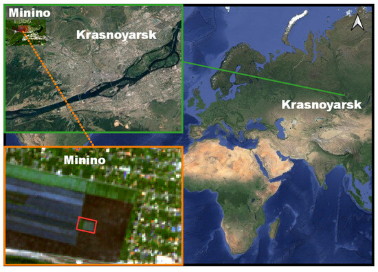
Figure 1.
Geographic location of the test field (red rectangle).
The topsoil of the test field is represented by clay loam soils with a clay content of 37–39%. The characteristics of the soil horizons are given in Table 1.

Table 1.
Soil characteristics of the test field.
Two cycles of measurements in the MHz- and GHz-frequency ranges were carried out on 25 August and 3 September 2023, respectively, in neighboring plots (2 × 2 m) of the test field. The following parameters were measured at each plot: RMS height and correlation length of soil surface roughness (after the complete cutting of plants), soil moisture, fresh and dry AGB, and canopy height. Roughness parameters were calculated from a digital elevation model (DEM) over five different linear profiles (length of ~1 m) drawn along the soil surface with different azimuths. The DEMs of the plots were constructed using the photogrammetric method (photographing with AIR 2S (DJI, Shenzhen, China) from a height of 2 m at various azimuthal angles). Local coordinates were assigned by a three-dimensional scale ruler (made of mutually perpendicular wooden blocks with a length of 40 cm and 1 m, with a cross-section of 19 × 40 mm) placed on the soil surface. The error in measuring soil surface roughness (<0.4 cm) was estimated as the RMS height along two linear profiles, drawn along the absolutely flat top surfaces of a wooden scale ruler. Soil moisture was measured at ~30 points in each plot using a GS3 (Decagon, San Francisco, CA, USA) sensor (sensor rods piercing the soil surface vertically, down to a depth of 5 cm). The effective thickness of the layer for moisture measurement was ~6–7 cm. The factory calibration of the GS3 sensor for mineral soils was used. Vegetation AGB was measured over entire plots using the thermostat-weight method. Canopy height was measured with a ruler at 10 points on each field plot.
2.2. Methodology of Remote Sensing Measurement
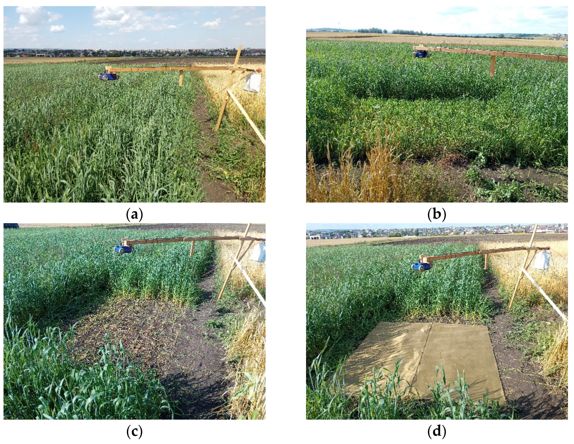
During the long process of vegetation growth, the soil’s surface roughness and moisture levels change. These changes constitute additional, uncertain variables that complicate the analysis of remote sensing data. In this paper, both sets of one-day experiments on the contactless GPR remote sensing of wheat were carried out while the moisture and roughness of the soil surface remained unchanged. At the same time, the sequential cutting-down of the wheat canopy (from the top to the soil surface in small layers of 10–20 cm) provided an opportunity to study the distortion of time shapes (amplitudes), propagation delay times, and spectral amplitude (reflection coefficient) of GPR impulses, depending on the height and biomass of the canopy. A monostatic nadir radar scheme was used for remote sensing in the MHz- and GHz-frequency ranges. The OKO-3 GPR with an AB-900M3 antenna unit (Geotech LLC, Moscow, Russia) was used as the source and receiver of impulses in the MHz-frequency range [51]. Continuous-time operating mode of OKO-3 GPR was used, with 1024 as the number of samples per scan and a time range of 32 ns. To generate impulses in the GHz-frequency range, a P6-59 horn antenna (JSC “NNRPA n.a. M.V. Frunze”, Nizhny Novgorod, Russia) [52] and a FieldFox N9917B 18GHz (Keysight, Colorado Springs, CO, USA) vector network analyzer (VNA) were used, adopting the method described in Refs. [53,54,55]. The VNA was initialized with the following presets: start and stop scan frequencies—0.5 GHz and 7.0 GHz, IF bandwidth—3 kHz, sweep resolution—4001 points, and output power—high (5 dBm). Before measurement, calibration of the VNA was performed with a standard mechanical calkit (Full 1-port Cal, 85518A, Type-N-50 Ohm) after a 15-minute warm-up time. The antennas were hung over the soil at fixed heights of 1.15 m (OKO-3 GPR) and 1.57 m (VNA), respectively, during the experiments. The progress of the experiments is shown in Figure 2 and Figure 3.
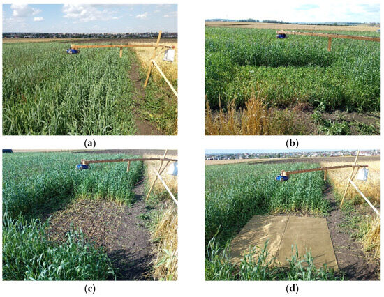
Figure 2.
(a–d) The process used in the experiment on the remote sensing of the wheat canopy in the MHz-frequency range with an OKO-3 GPR (23 August 2023); (d) measurement over a metal screen. Free space calibration is not shown.

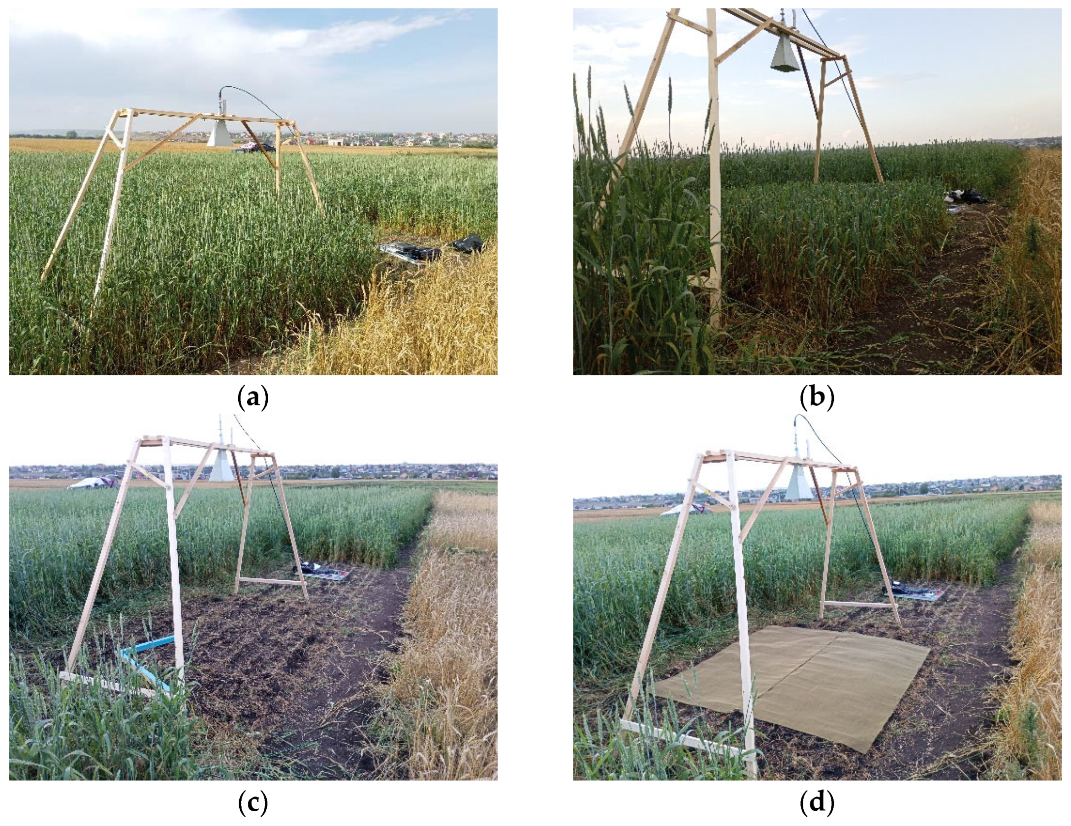
Figure 3.
(a–d) The process used in the experiment on the remote sensing of the wheat canopy in the GHz-frequency range with a horn antenna (3 September 2023); (d) measurement over a metal screen. Free space calibration is not shown.
Calibration relative to a metal screen (brass mesh), performed according to the method used in Refs. [53,54,55], made it possible to carry out absolute measurement of the GPR impulse amplitudes and the reflection coefficient. In the case of a horn antenna, based on the spectral measurements of the reflection coefficient S11(f) at the antenna terminals by VNA, the GPR impulse was synthesized based on the following formulas:
where t is the time, Ssv,ref(f) = Kα(f)S11(f), the smoothing Gaussian spectral window function was chosen as Kα(f) = exp(−0.5[(f − f0)/α]2), α = Δf/, fmin and fmax are the frequency limits of S11(f) measurement; and are the analytical signal and envelope of the impulse ssv,ref(t), reflected from the layered structure of vegetation–soil cover (sv) and a metal screen (ref.); index «0» corresponds to the free space measurements; is the maximum of the impulse envelope, reflected from a metal screen. The average frequency and spectrum half-bandwidth of the window function were set as equal to f0 = 3.0 GHz and Δf = 1.15 GHz, respectively (the choice of such parameters is justified at the end of this paper). To reduce the influence of the direct wave, the spectrum S0(f) was measured with the antennas oriented to the zenith (free-space calibration), and it was then subtracted from the spectra Ssv,ref(f). In the case of the OKO-3 GPR antenna used, an inverse Fourier transform was performed, the spectrum of the GPR impulses Ssv,ref,0(f) was found, and then a similar calibration method to (1)–(2) was performed.
The complex reflection coefficient from the layered structure of vegetation–soil cover was calculated in the spectral region as Rsv(f) = Ssv(f)/Sref(f). The modules of the reflection coefficient from the layered structure of vegetation–soil cover were calculated at the average frequency of the GPR impulses |Rsv(f0)| = and in the time domain |Rsv(t)| = .
2.3. Model of the Reflection Coefficient and Dielectric Model of the Canopy
The spectrum of the complex reflection coefficient of a plane wave that is normally incident to the soil surface, which is covered with vegetation, can be written in the following form:
where Rac and Rcs are the Fresnel reflection coefficients from the air–canopy and canopy–soil interfaces, respectively; ; εcan is the RCP of the vegetation canopy; hcan is the height of the canopy; εs is the RCP of soil. In model (3), the phenomena of wave scattering on individual elements of plants, as well as multiple wave reflections between the air–canopy and canopy–soil interfaces were neglected. The RCP of soil is εs = εs(f, W, ρd, C), where W is the volumetric water content, ρd is the dry bulk density, and C is the clay fraction by weight, which was calculated using the Mironov model [56]. The two-relaxation Mironov dielectric model is created based on the RCP data for 6 types of mineral soil samples, measured in the frequency range of 0.04–26.5 GHz. The clay, sand, and silt fractions in these soil samples varied from 7% to 76%, from 0% to 55%, and from 11% to 93%, respectively.
The RCP of the canopy is calculated based on the refractive mixing dielectric model [37,57,58] of air and vegetation [59,60]:
where = ncan,v + i κcan,v, ncan,v and κcan,v are the refractive index and normalized attenuation coefficient of the canopy (can) and vegetation material (v), and is the volume fraction of vegetation material in the canopy. The RCP of vegetation εv= εv(f, , ), as a function of frequency, salinity (), and the weight (mv) of plant fluid, was calculated based on the dielectric model [61]. The volumetric fraction of vegetation material in the canopy is given by the equation:
where and are the volume of vegetation material and the test volume of the canopy, V = A·hcan, is the density of wet vegetation material, A is the area under the test canopy, and B in [kg/m2] is the fresh AGB. Gravimetric moisture content in the canopy is given by the equation , where and are the weights of wet and dry plants.
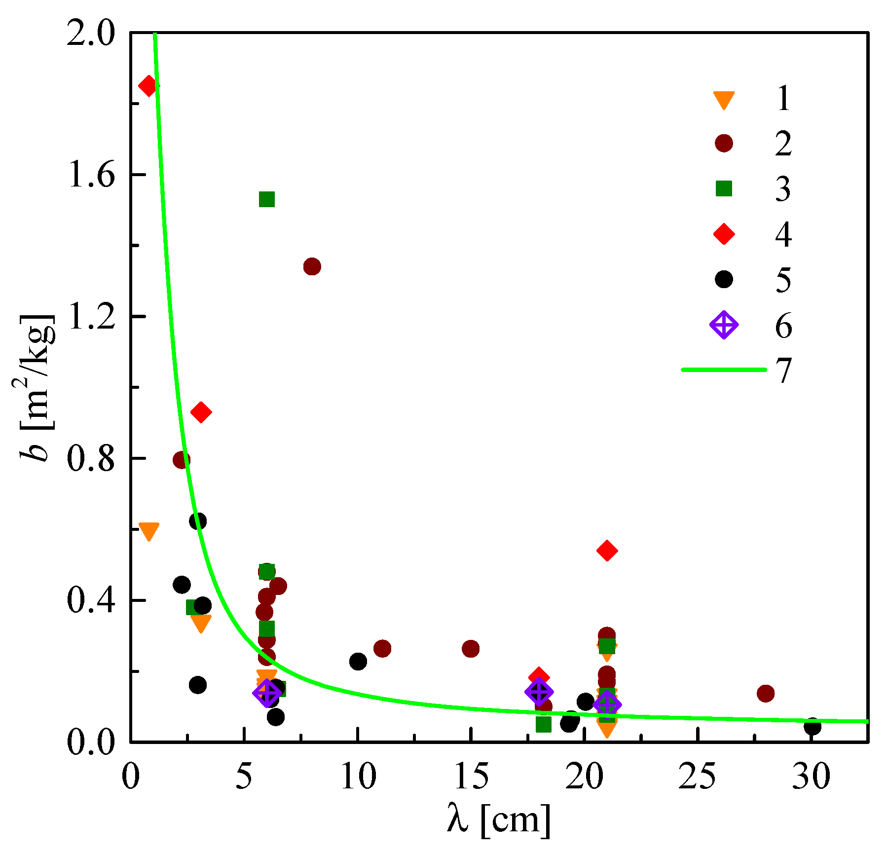
The validity of the refractive mixing model (4) for assessing the vegetation b-factor depending on frequency was checked. The brefr-factor was estimated based on model (4) from the optical thickness equation τrefr = brefr·B = 2·k0·hcan·κcan(f), using experimental data [62,63] on height, water content, and fresh plant biomass. Conversely, the values of brad-factor were taken from radiometric-based measurements of the optical thickness of vegetation cover with different AGB values [60,64,65,66]. Figure 4 shows that the dispersion of the brad-factor decreases with increasing wave-length, which is a consequence of the predominant wave’s attenuation prevails over the scattering phenomenon in the vegetation cover. In general, good agreement between the theoretical estimates of the b-factor based on the refractive model (4) and the experimentally measured ones [60,64,65,66] can be observed. Furthermore, model (4) will be used to estimate the fresh AGB of the vegetation canopy.
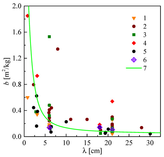
Figure 4.
Lambda dependency of the b-factors: 1—corn [64,65], 2—soybean [64,65,66,67], 3—wheat [64,65], 4—alfalfa [64,65], 5—wheat grains [60], 6—cereals, and sorghum [66] are brad-factors, estimated based on radiometric measurements, and the 7–brefr-factor, calculated based on the refractive mixing model (4).
2.4. Algorithm for Measuring Soil Moisture and Surface Roughness, Canopy Height, and Biomass
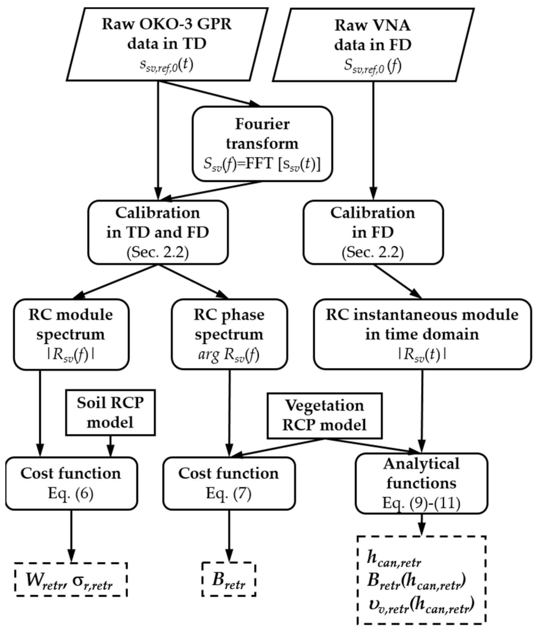
Two algorithms for retrieving soil geophysical and vegetation biometric parameters are considered in the MHz- and GHz-frequency ranges. In the first algorithm, based on OKO-3 measured GPR impulses in MHz-frequency range, (a) soil surface moisture and roughness, and (b) fresh AGB are retrieved from the informative criterion of |Rsv(f)| and arg Rsv(f), respectively (see Figure 5). The inverse problem of soil moisture and soil surface roughness retrieval can be formulated as:
where and are the measured and calculated spectra of the module of reflection coefficient for a given AGB.

Figure 5.
Flowchart of algorithms used for soil geophysical and canopy biometric parameters, based on the measured OKO-3 GPR data in the time domain (TD) and VNA data in the frequency domain (FD).
The influence of canopy on the attenuation of an impulse, reflected from the soil surface, is neglected; it will be assumed in model (3), where Rac = 0 and hcan = 0 m. The soil dry density and clay content are set as equal to ρd = 1.1 g/cm3 and C = 39%, respectively (see Table 1). The vegetation biomass can be found by minimizing the functional:
where , and the phases of the reflection coefficients Rac(f) and Rcs(f) in Formula (3) will be neglected. The density of fresh vegetation material is significantly determined by the water content; thus, we will assume that ρv ≅ ρw·mv, where ρw ≈ 103kg/m3 is the water density in normal conditions. The gravimetric moisture content in the vegetation during the experiment was approximately equal to mv ≈ 80%, with a salinity of msalt = 10‰. Also, when solving Formula (7), we assume that hcan is a known value (either measured experimentally, or this value was obtained during minimization (6)). The inverse problems (6) and (7) were solved using the Levenberg–Marquardt algorithm [68].
In the second algorithm, based on the VNA spectral measurements in the GHz-frequency ranges (see Figure 5), neglecting the influence of the reflected wave from the soil surface (see Formula (3) at Rcs≡0), it is possible to estimate the instantaneous values of the refractive index in the internal structure of the canopy ncan,retr(t), based on the Fresnel equation:
where |Rsv(t)| can be interpreted as the instantaneous value of the module of the reflection coefficient (see the definition at the end of Section 2.2). Note that Formula (3) does not take into account the scattering phenomenon, which can lead to an overestimation of ncan,retr(t), calculated using Formula (8). Then, using Formulas (4) and (8), the volumetric content of the vegetation elements Δvv,retr(t) in the canopy at time t can be estimated:
where nv(f0) is the refractive index of the vegetation material at the central frequency of the GPR impulse. The time scale t (arrival impulses) can be recalculated into the absolute values of the vertical coordinate z, using the known values of ncan,retr(t):
where z = 0 m corresponds to the soil surface; t0 is the arrival time of the maximum impulse envelope, reflected from the metal screen. Based on the measured arrival time of the first impulse, tac, reflected from the air–canopy interface, the height of the canopy can be estimated from Formula (10) as zmax(t = tac)⇒ hcan,retr. Note that based on Formula (10), the instantaneous values of the refractive index and the volumetric content of vegetation elements can be expressed as a function of the vertical coordinate z or hcan,retr. Then, using the integral representation of Equation (5), the profile B(z) of fresh AGB can be estimated:
where, as before, it is assumed that ρv ≅ ρw·mv (mv ≈ 80%).
3. Results
3.1. Experiment in the MHz-Frequency Range
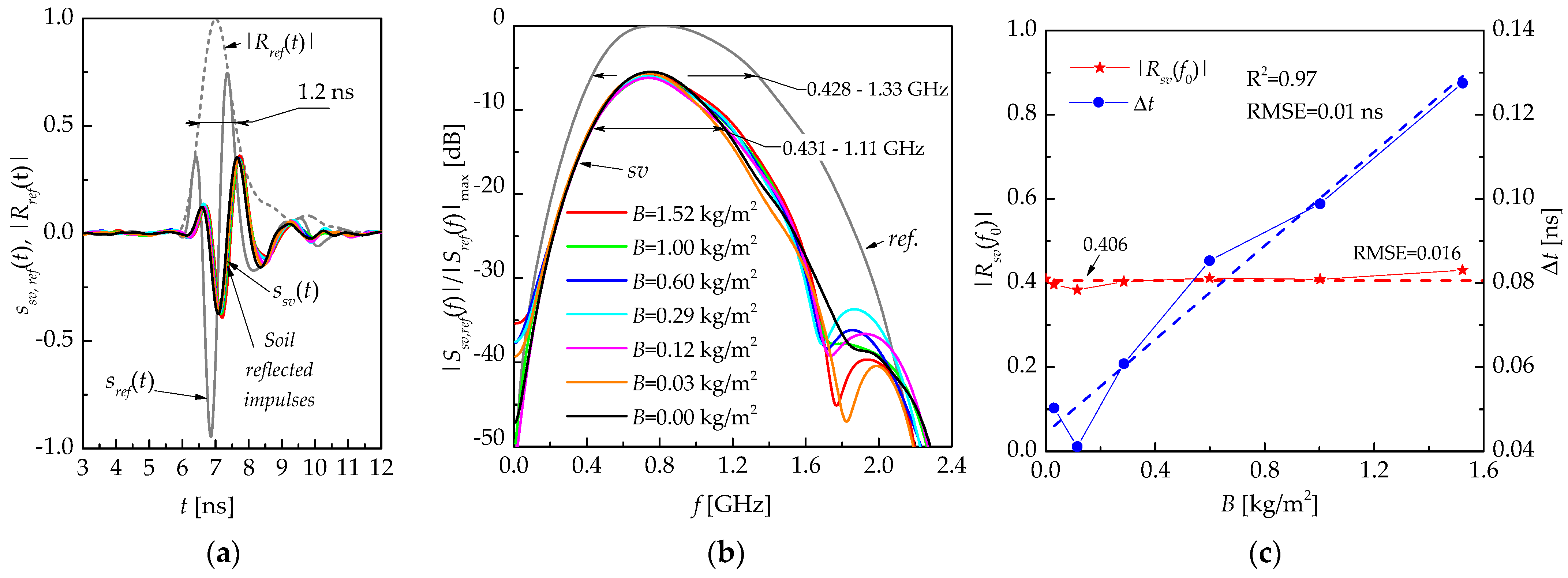
During the experiment conducted on 23 August 2023, an impulse with a duration of ΔτMHz = 1.2 ns (at the 0.5 level of the maximum envelope), with a spectrum bandwidth from 428 MHz to 1.33 GHz (at a level of −6 dB) and a central frequency of 750 MHz, was used for remote sensing of the wheat canopy. The normalized time shape of the GPR impulse, reflected from the metal screen sref(t) (brass mesh 2 × 2 m), together with the normalized envelope of the analytical signal , is shown in Figure 6a (see the solid and dashed gray curves, respectively). Following the methodology, the amplitude of the GPR impulses, reflected from the vegetation–soil cover, was normalized by the maximum envelope of the GPR impulse, reflected from the metal screen . The measured time shapes of the impulses ssv(t) for the cut-down canopy, calculated layer by layer from the top to the soil surface, are shown in Figure 6a (see the colored curves). The modules of the normalized spectra of GPR impulses, reflected from the metal screen |Sref(f)|, and the vegetation–soil cover |Ssv(f)| are shown in Figure 6b. As the wheat is cut down layer by layer, the maximum variations in the measured modulus of the reflection coefficient |Rsv(f0)| relative to the average value do not exceed ~6% (see Figure 6c).
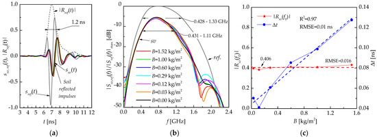
Figure 6.
(a) Time shapes of the GPR impulse MHz-frequency range, reflected from the vegetation–soil cover ssv(t) (color lines) and metal reflector sref(t) (gray solid line), with the normalized envelope of impulse, reflected from the metal screen |Rref(t)|= (gray dashed line); (b) the corresponding normalized module of the impulse spectrum |Ssv,ref(f)|; (c) the module of the reflection coefficient |Rsv(f0)| and the delay time Δt (calculated from the maximum envelopes) of GPR impulses (see Figure 6a), depending on the measured fresh AGB value calculated by the thermostat-weight method.
It can be seen that against the background of the GPR impulses, which are reflected from the soil surface, the impulses reflected (scattered) by the vegetation cover are not identified. The delay time when the GPR impulses pass twice through the canopy increases from ~0.04 ns to ~0.13 ns as the fresh AGB value increases from 0 kg/m2 to 1.52 kg/m2 (see Figure 6c). The time delay of the impulses was calculated as the difference between the arrival times of the impulse’s envelopes’ maxima, as reflected from the metal screen and the soil surface. The impulse time delay of 0.04 ns at zero for fresh AGB (see Figure 6c) was caused by a calibration error because the metal screen lay on soil with a roughness slightly higher than the average level of the air–soil interface.
The data presented in Figure 6c shows an unambiguous linear correlation between the time delay Δt of the impulse reflected from the soil surface and the fresh AGB of the wheat. Moreover, both the time shapes and the amplitudes of the reflected impulses from the soil surface are practically independent of fresh AGB (up to 1.52 kg/m2) and a canopy height up to 87 cm. In contrast to the module of reflection coefficient |Rsv(f0)| (see Figure 6c), measured from the maximum of the envelopes’ reflected impulses (see Figure 6a), the spectrum of the complex reflection coefficient Rsv(f) contains a frequency-dependent relationship with soil surface roughness and vegetation biomass.
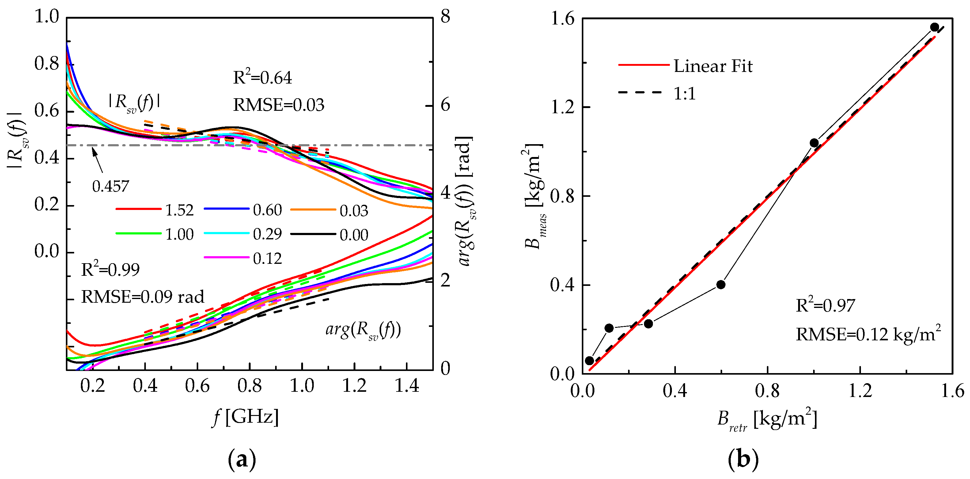
Taking advantage of the first algorithm (see Section 2.4, Equations (6) and (7)), the canopy biomass, as well as soil moisture and roughness, were retrieved from the measured complex reflection coefficient. The measured and calculated spectra , with the optimally established parameters are shown in Figure 7a. The retrieved fresh AGB values relative to the measured ones are shown in Figure 7b. The retrieved value of volumetric soil moisture Wretr = 23.4 ± 2.6%, with an absolute error of 3.3% (relative error 16.4%), coincides with the measured in situ value of 20.1 ± 3.7% by the Decagon GS3 sensor in 0–6 cm of topsoil on the test plot. The retrieved value of σr,retr= 1.4 ± 0.3 cm is, on average, overestimated by 0.5 cm relative to the measured in situ value of 0.9 ± 0.4 cm, due to the fact that model (3) does not take into account the wave-scattering phenomenon found on plant elements in the canopy.
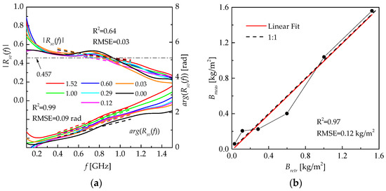
Figure 7.
(a) The measured (solid lines) and retrieved (dash lines) modules and arguments of the spectrum of reflection coefficients; (b) the correlation between measured and retrieved fresh AGB values. The optimally found parameters while solving the inverse problem (6) were Wretr = 23.4 ± 2.6% and σr,retr= 1.4 ± 0.3 cm. The color scheme of solid and dashed color lines is the same (various colors of lines correspond to the different values for fresh AGB in [kg/m2]).
The average value of the module of reflection coefficient is 0.457 (see Figure 7a, gray dash-dotted line), calculated based on the optimally found parameters Wretr and σr,retr in the spectrum bandwidth of impulse, and coincides with the average value of |Rsv(f0)| = 0.406 (see Figure 6c) at an absolute error of 5.1% (relative error 12.3%), measured based on the maximum impulse amplitudes. Figure 7a shows that model (3) in the spectrum bandwidth of the GPR impulse describes with good accuracy the measured values of the modulus of the reflection coefficient. The retrieved values for canopy biomass after each cutting-down, with a high value for the determination coefficient, coincide with the measured ones (see Figure 7b).
3.2. Experiment in GHz-Frequency Range
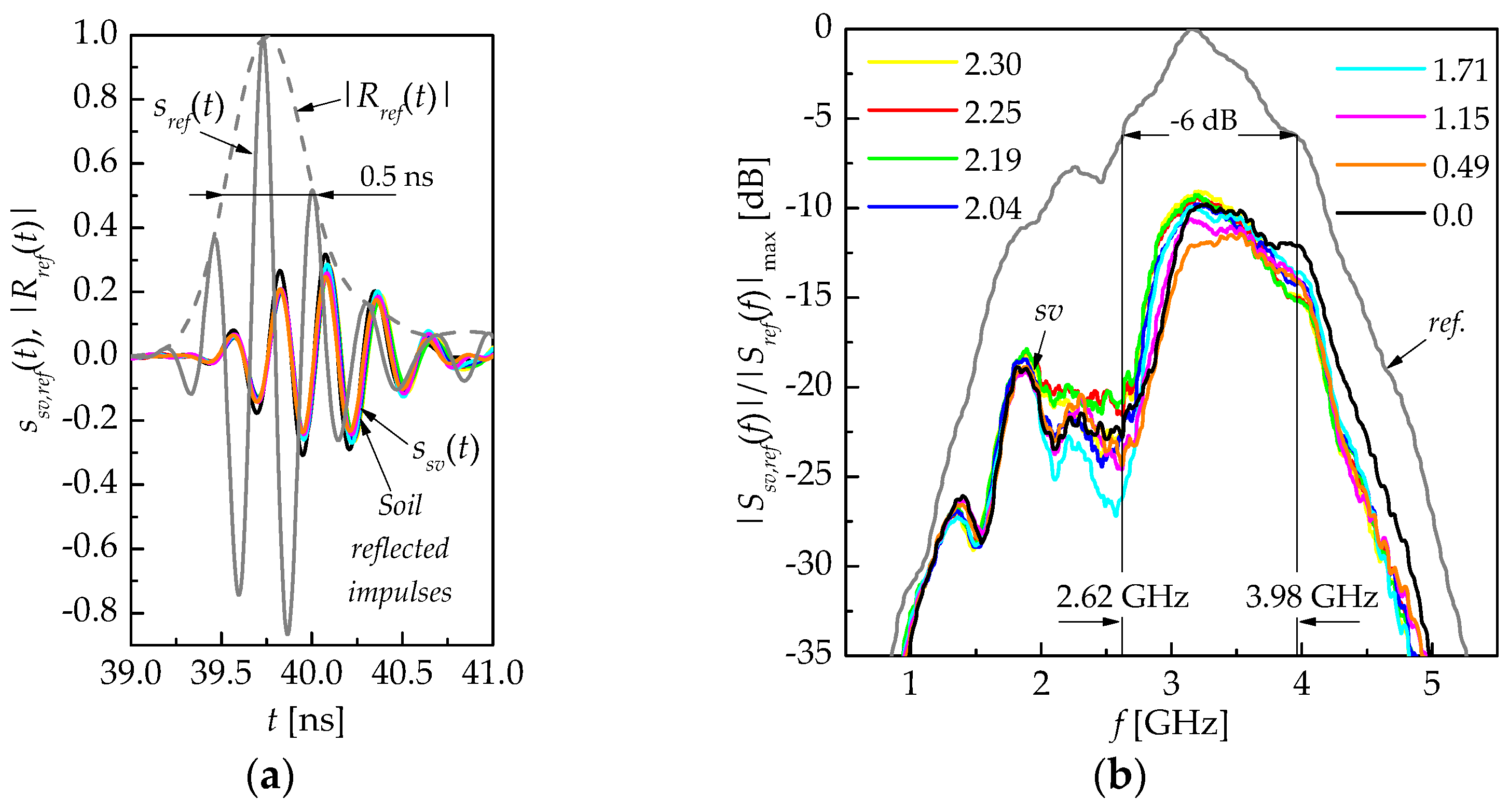
During the experiment on 3 September 2023, an impulse with a duration of ΔτGHz = 0.5 ns (at a 0.5 level of the maximum envelope, see Figure 8a) with a bandwidth of 1.36 GHz (at a level of −6 dB, from 2.62 GHz to 3.98 GHz) and 2.16 GHz (at a level of −10 dB, from 2.02 GHz to 4.18 GHz), with an average frequency of 3.2 GHz (see Figure 8b) was used for the remote sensing of the wheat canopy at another test plot. The normalized time shape sref(t) and envelope of the GPR impulse, reflected from a metal screen (brass mesh 2 × 2 m), is shown in Figure 8a (see the solid and dashed gray curves, respectively). The timeline in Figure 8a starts from 39.0 ns for analyzing the impulses reflected from the soil surface. In accordance with the methodology, the amplitude of the impulses reflected from the vegetation–soil cover was calibrated by normalizing to the maximum envelope of the impulse, as reflected from the metal screen . The measured time shapes of the impulses are shown in Figure 8a (see colored curves) as the wheat cut down layer by layer from the top to the soil surface. The normalized impulse spectra, reflected from the metal screen |Sref(f)| and from the vegetation–soil cover |Ssv(f)|, are shown in Figure 8b.
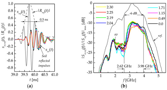
Figure 8.
(a) Time shapes of the GPR impulses GHz-frequency range, reflected from the vegetation–soil cover ssv(t) (color lines) and metal reflector sref(t) (gray solid line), normalized envelope of impulse, reflected from the metal screen |Rref(t)| (gray dashed line); (b) the corresponding normalized module of the impulse spectrum |Ssv,ref(f)|. Various colors of lines correspond to the different values of fresh AGB in [kg/m2]. The color scheme is the same as in the pictures.
As the wheat is cut down and its fresh AGB value decreases from 2.30 kg/m2 to 0.0 kg/m2, the time delay of the impulses reflected from the soil surface decreases slightly by 0.03 ns (from 40.09 ns to 40.12 ns), and the amplitude increases by 1.3 dB (see Figure 8a). Figure 8b shows that the spectral amplitudes of impulse |Ssv(f)|, reflected from the vegetation–soil cover, in its bandwidth do not have a clear linkage with a decrease or increase in AGB. This evidence does not allow the use of impulses in the GHz-frequency range, reflected from the soil surface, for the reliable measurement of AGB.
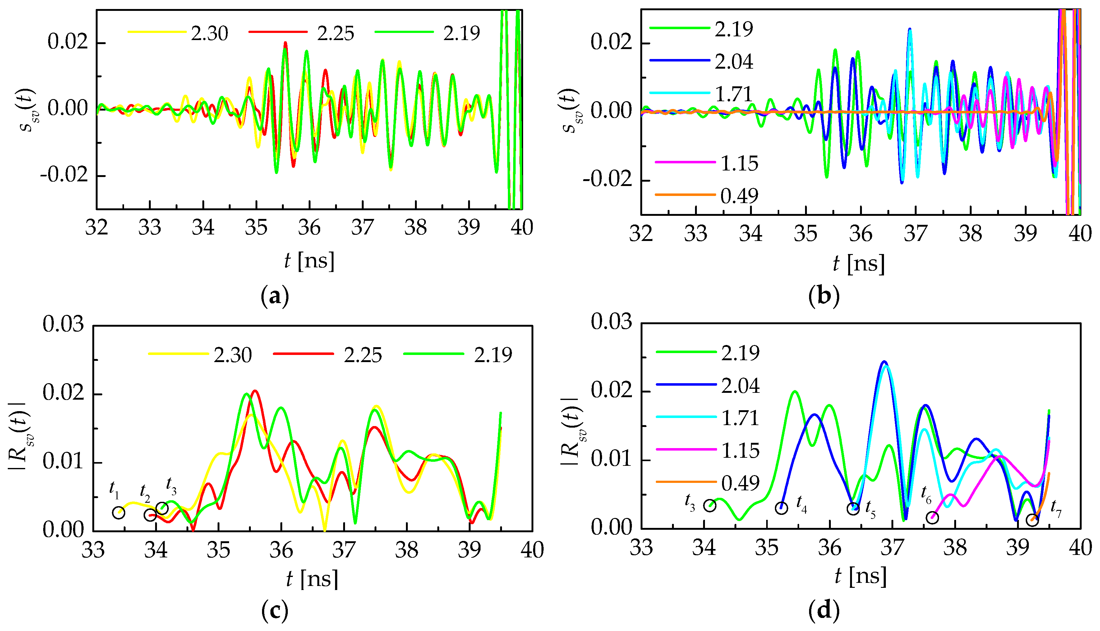
At the same time, shown much more confidently compared to Refs. [34,35,36], Figure 9a,b reveals the impulses, reflected (scattered) not only by the air-canopy interface but also from internal plant elements in the canopy, located at different heights from the soil surface (time interval from ~32 ns to ~39.5 ns, the arrival time of the maximum envelope of the impulse, when reflected from the soil surface is t0 = 39.77 ns). The normalized envelopes of the impulses reflected (scattered) by the canopy (see Figure 9c,d; time is from ~32 ns to ~39.5 ns) can be interpreted as the instantaneous value of the module of the reflection coefficient |Rsv(t)|.
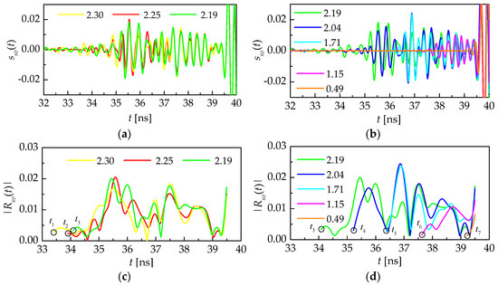
Figure 9.
(a,b) Normalized time shapes of impulse ssv(t), reflected from the vegetation–soil cover and (c,d) their envelopes as wheat is cut down from the top to the soil surface. In the legend, the numbers indicate fresh AGB in [kg/m2], measured in situ by the thermostat–weight method. The key for the black circles will be made clear further on.
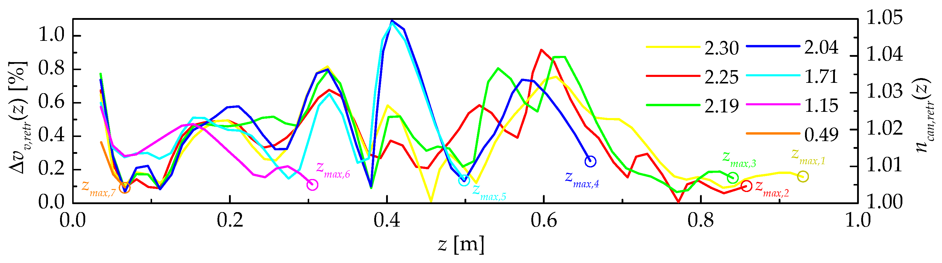
As a result, based on Equations (8)–(10) and the data shown in Figure 9c,d, the values of ncan,retr(z) and Δvv,retr(z) can be calculated (Figure 10).
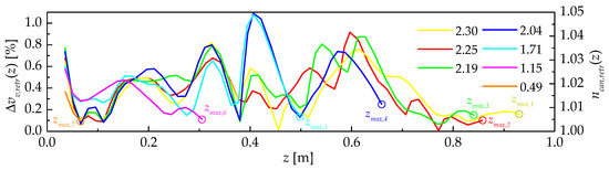
Figure 10.
Retrieved local values of the volumetric contents of vegetation elements Δvv,retr(z) and the refractive index ncan,retr(z) in the canopy. The numbers in the legend indicate the values of fresh AGB in [kg/m2], measured by the thermostat-weight method.
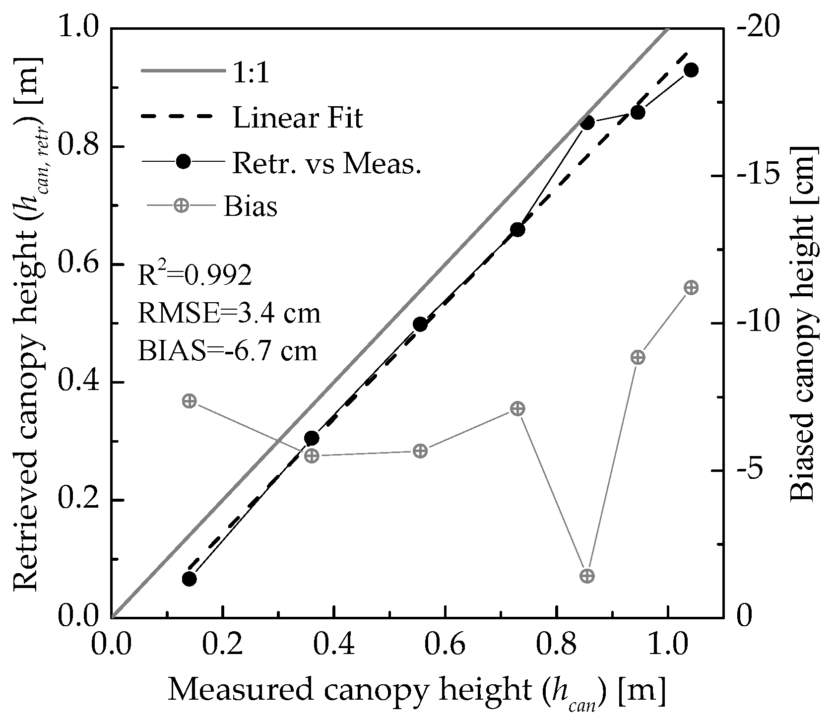
Note that when calculating the dependencies (see Figure 10), the time interval (see Figure 9c,d) on the right was limited to 39.52 ns = t0 − ΔτGHz/2. The time interval on the left was limited by the smallest value of the impulse arrival time (see Figure 9c,d, t1, …, t7), found from the criterion: ncan,retr(t) > . This criterion means a 10% excess of ncan,retr(t) fluctuations relative to the average initial level (this average value was assessed in the interval from 32 to 33 ns). As the canopy was cut down from the top to the soil surface, the position of the air-canopy interface was confidently identified, based on the criteria described above (see the black circles in Figure 9c,d, t1,…,t2, and the color circles in Figure 10, zmax,1,…, zmax,7). The hcan,retr = zmax,1,…, zmax,7 values found in this way are underestimated by an average of 6.7 cm relative to the wheat height measured with a ruler, and they correlate with each other, with R2 = 0.992 and RMSE = 3.4 cm (see Figure 11). As the canopy height increases, the measured heights tend toward more underestimation, up to −11.3 cm.

Figure 11.
Dependence of the retrieved data on the measured canopy heights.
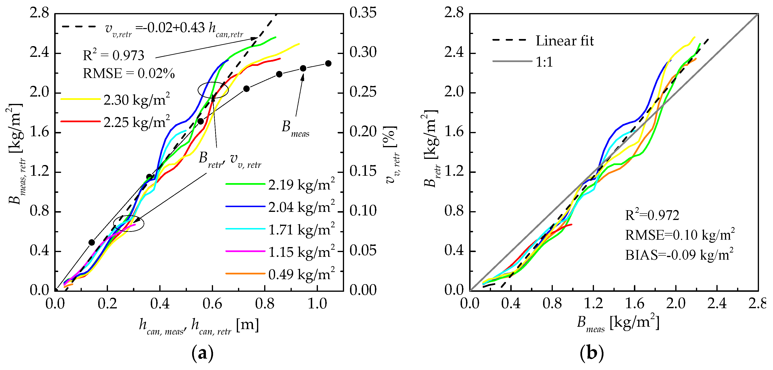
Figure 10 also shows that for six different cutting heights of vegetation, the shapes of ncan,retr(z) and Δvv,retr(z) are not random but systematically reproduce some characteristic layered structures of local heterogeneities (reflectors/scatters) in the canopy. The retrieved profiles of the fresh AGB values, using Equation (11), are shown in Figure 12a. It can be seen that the retrieved fresh AGB values (less than ~1 kg/m2) are underestimated, relative to the measured ones. An underestimation of Bretr is associated with an underestimation of hcan, retr (and, therefore, Δvv,retr). In addition, the relative error in hcan, retr and Δvv,retr retrieval increases as the canopy height decreases. When the amount of biomass becomes significant (more than ~1 kg/m2), apparently, the share of waves scattered by the plant elements increases, which is not taken into account in either the model of the reflection coefficient (3) or in the dielectric model of the canopy (4), which leads to an overestimation of Bretr. In general, a high coefficient of determination R2 = 0.972 and a relatively low error RMSE = 0.10 kg/m2 of the retrieved fresh AGB values relative to the measured ones are observed (see Figure 12b).
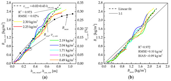
Figure 12.
(a) The retrieved Bretr (color lines) and measured Bmeas (line with black circles) for fresh AGB, depending on the retrieved hcan,retr and measured hcan,meas canopy heights, respectively; (b) correlation between the retrieved and measured fresh AGB values.
Due to the underestimation of retrieved canopy height, the retrieved fresh AGB value is also underestimated by 0.09 kg/m2 (see Figure 12b). Figure 12a also shows the possibility of estimating the volumetric content of fresh vegetation (as can be seen from (9)), which can be described by a linear dependence on the retrieved canopy height, with R2 = 0.973 and RMSE = 0.02% (see Figure 12a, dashed line). Apparently, this linear relationship is specific to each kind of plant and canopy texture.
4. Discussion
Single-day studies on the test plots when cutting down wheat made it possible to exclude the impact of soil moisture and surface roughness time-variation on the distortion of the time shape and spectrum of GPR impulses, which is a strong point for the proposed method. At the same time, the wheat was at the heading stage, which did not allow us to study the distortion of the time shapes and spectra of the GPR impulses throughout the growing period of the wheat. Future similar one-day studies are strongly recommended during the various vegetative phases to verify the proposed algorithms for measuring soil moisture, surface roughness, canopy height, and biomass. Since the OKO-3 GPR impulse (in the MHz-frequency range) weakly interacts with the canopy, this frequency band is suitable for the retrieval of soil moisture and surface roughness information. One of the significant disadvantages of the proposed method in the MHz-frequency range is its requirement of prior knowledge of the canopy height for biomass retrieval. The use of impulses in a GHz-frequency range allows us to solve this problem. To carry out measurements in the GHz-frequency range, the impulse parameters (see Section 2.2) were optimally chosen while solving the inverse problem by minimizing the norm of the difference between the measured and retrieved fresh AGB |Bmeas–Bretr|min (see Figure 13). Figure 13 shows that when the average frequency varies from 2.0 GHz to 3.5 GHz and the spectrum half-bandwidth varies from ~1.0 GHz to 1.5 GHz of GPR impulses, there is a minimum functional of |Bmeas–Bretr|. In accordance with the data shown in Figure 13, the spectrum half-bandwidth and center frequency for synthesizing the GPR impulse in the GHz-frequency range were chosen as Δf = 1.15 GHz and f0 = 3 GHz, respectively (see Section 2.2).
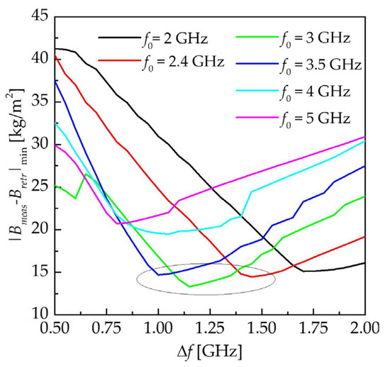
Figure 13.
Relief of the norm of the difference between measured and retrieved fresh AGB values in total for all wheat-height cuts (see Figure 12a), depending on the half-bandwidth Δf and the central frequency f0 of the Gaussian window function (see Section 2.2 and the text for Formulas (1)–(2)).
The synthesized impulse in the GHz-frequency range is apparently less susceptible to scattering by vegetation elements, compared to volumetric reflection and attenuation. As a result, the observed reflection/scattering of the GPR impulse in the GHz-frequency range, as shown, can be described by the model of the reflection coefficient of a plane wave (3) and the refractive mixing permittivity model of the canopy (4). Note that the phase-frequency method was not used for AGB retrieval in the GHz-frequency range because the impulse reflected from the soil surface should be eliminated by a time-domain window filter, which will introduce significant distortions into the reflected impulses from the bottom of the canopy. In this regard, in the GHz-frequency range, the most convenient method was the analysis of impulses reflected/scattered by the canopy in the time domain. In general, the proposed method (with combined impulses in the MHz- and GHz-frequency ranges) allowed us not only to retrieve the values for Bretr, Wretr, and hr,retr with significant accuracy for practical use but even the profiles of the canopy biomass and volumetric contents of vegetation elements.
It is also worth mentioning that placing radar units on a UAV will introduce special aspects to the processing and interpretation of radiated and reflected GPR impulses. Firstly, the impulse that is radiated and received by the UAV’s radar will be distorted by the UAV’s structural components, which are situated in the near-field region of the radar antenna. Secondly, the amplitude of the impulse reflected from the vegetation–soil layer will depend on the flight altitude of the UAV. The effect of these factors on the distortion of the time shape and the amplitude of the sensing impulses can be eliminated through the calibration of the UAV’s radar, for example, as proposed in Refs. [53,55]. The findings from this study should be comparable when measured with a UAV flying at varying altitudes, with adjustments made for the corresponding in situ spatial averaging within the footprint area (requiring specific additional experimental validation).
5. Conclusions
This paper investigates the possibilities of broadband electromagnetic impulses in MHz- and GHz-frequency ranges for the remote sensing of soil moisture and the height and biomass of a wheat canopy. The broadband impulse of the MHz-frequency range (a duration of 1.2 ns) interacts negligibly with the wheat canopy (in biomass up to 1.5 kg/m2, height up to 87 cm) and can be used for the remote sensing of soil moisture under such a canopy. In this case, variations in the impulse delay times (~0.09 ns) can also be neglected when the wheat biomass varies. It is shown that in the MHz-frequency range, a simple model of the frequency-dependent reflection coefficient (with a normal distribution of soil surface roughness) allows us to retrieve information on both soil moisture and the RMS heights of soil surface roughness under the wheat canopy. In the GHz-frequency range, the choice of an impulse with a duration of ~0.5 ns (average frequency of 3 GHz and spectrum half-bandwidth of 1.2 GHz) made it possible to confidently detect not only the time delay between impulses, reflected from the air–canopy and canopy–soil interfaces, but also the internal layered structure in the wheat canopy (fresh AGB up to 2.3 kg/m2). It is shown that the height of wheat (up to 104 cm) can be estimated with R2= 0.99 and a bias of −7 cm, based on measuring the time delays of GHz-frequency range impulses, as reflected from the air–canopy and canopy–soil interfaces. In this case, the vertical profile of fresh AGB with R2 = 0.97 can be retrieved using the refractive mixing model of the canopy. The combination of the impulses of two different frequency ranges will, in the future, make it possible to create UAV-based reflectometers for the simultaneous mapping of soil moisture, height, and vegetation biomass for precision farming systems.
Author Contributions
Conceptualization, methodology, investigation, experiments, calculation, writing—original draft preparation, review and editing, project administration, and funding acquisition, K.M.; soil dielectric modeling and calculation and experiments, S.F. and A.K.; experiments, J.L.; agrofield resources and experiments, A.L. and V.R. All authors have read and agreed to the published version of the manuscript.
Funding
The investigation was supported by the Russian Science Foundation and the Krasnoyarsk Regional Science Foundation, project No. 22-17-20042.
Data Availability Statement
The original contributions presented in the study are included in the article, further inquiries can be directed to the corresponding author.
Acknowledgments
For their assistance in conducting the experiments, we thank Mikhail Mikhaylov (engineer at the Laboratory of Radiophysics of the Earth Remote Sensing Kirensky Institute of Physics Federal Research Center, KSC Siberian Branch, Russian Academy of Science).
Conflicts of Interest
The authors declare no conflicts of interest.
References
- Khang, A. (Ed.) Handbook of Research on AI-Equipped IoT Applications in High-Tech Agriculture; IGI Global: Hershey, PA, USA, 2023; 473p. [Google Scholar]
- Zaman, Q. (Ed.) Precision Agriculture Evolution, Insights and Emerging Trends; Academic Press: Cambridge, MA, USA; Elsevier: Amsterdam, The Netherlands, 2023; 260p. [Google Scholar]
- Cognitive Technologies. Available online: https://cognitivepilot.com/breaking-news/vopros-otvet-o-rabote-novogo-avtopilota-na-traktorah-kirovecz-k-7m/ (accessed on 1 July 2024).
- Wang, D.; Li, R.; Zhu, B.; Liu, T.; Sun, C.; Guo, W. Estimation of Wheat Plant Height and Biomass by Combining UAV Imagery and Elevation Data. Agriculture 2023, 13, 9. [Google Scholar] [CrossRef]
- Kümmerer, R.; Noack, P.O.; Bauer, B. Using High-Resolution UAV Imaging to Measure Canopy Height of Diverse Cover Crops and Predict Biomass. Remote Sens. 2023, 15, 1520. [Google Scholar] [CrossRef]
- Shafiee, S.; Mroz, T.; Burud, I.; Lillemo, M. Evaluation of UAV multispectral cameras for yield and biomass prediction in wheat under different sun elevation angles and phenological stages. Comput. Electron. Agric. 2023, 210, 107874. [Google Scholar] [CrossRef]
- Harkel, J.T.; Bartholomeus, H.; Kooistra, L. Biomass and Crop Height Estimation of Different Crops Using UAV-Based Lidar. Remote Sens. 2020, 12, 17. [Google Scholar] [CrossRef]
- Bates, J.S.; Montzka, C.; Schmidt, M.; Jonard, F. Estimating Canopy Density Parameters Time-Series for Winter Wheat Using UAS Mounted LiDAR. Remote Sens. 2021, 13, 710. [Google Scholar] [CrossRef]
- Zhang, Y.; Yang, Y.; Zhang, Q.; Duan, R.; Liu, J.; Qin, Y.; Wang, X. Toward Multi-Stage Phenotyping of Soybean with Multimodal UAV Sensor Data: A Comparison of Machine Learning Approaches for Leaf Area Index Estimation. Remote Sens. 2023, 15, 7. [Google Scholar] [CrossRef]
- Wang, T.; Liu, Y.; Wang, M.; Fan, Q.; Tian, H.; Qiao, X.; Li, Y. Applications of UAS in Crop Biomass Monitoring: A Review. Front. Plant Sci. 2021, 12, 616689. [Google Scholar] [CrossRef]
- Tang, Z.; Parajuli, A.; Chen, C.J.; Hu, Y.; Revolinski, S.; Medina, C.A.; Lin, S.; Zhang, Z.; Yu, L.-X. Validation of UAV-based alfalfa biomass predictability using photogrammetry with fully automatic plot segmentation. Sci. Rep. 2021, 11, 3336. [Google Scholar] [CrossRef] [PubMed]
- Liu, T.; Zhu, S.; Yang, T.; Zhang, W.; Xu, Y.; Zhou, K.; Sun, J. Maize height estimation using combined unmanned aerial vehicle oblique photography and LIDAR canopy dynamic characteristics. Comput. Electron. Agric. 2024, 218, 108685. [Google Scholar] [CrossRef]
- Pittman, J.J.; Arnall, D.B.; Interrante, S.M.; Moffet, C.A.; Butler, T.J. Estimation of Biomass and Canopy Height in Bermudagrass, Alfalfa, and Wheat Using Ultrasonic, Laser, and Spectral Sensors. Sensors 2015, 15, 2920–2943. [Google Scholar] [CrossRef]
- Bertalan, L.; Holb, I.; Pataki, A.; Négyesi, G.; Szabó, G.; Szalóki, A.K.; Szabó, S. UAV-based multispectral and thermal cameras to predict soil water content–A machine learning approach. Comput. Electron. Agric. 2022, 200, 107262. [Google Scholar] [CrossRef]
- Guan, Y.; Grote, K. Assessing the Potential of UAV-Based Multispectral and Thermal Data to Estimate Soil Water Content Using Geophysical Methods. Remote Sens. 2024, 16, 61. [Google Scholar] [CrossRef]
- Lu, F.; Sun, Y.; Hou, F. Using UAV Visible Images to Estimate the Soil Moisture of Steppe. Water 2020, 12, 2334. [Google Scholar] [CrossRef]
- Kim, K.Y.; Zhu, Z.; Zhang, R.; Fang, B.; Cosh, M.H.; Russ, A.L.; Dai, E.; Elston, J.; Stachura, M.; Gasiewski, A.J.; et al. Precision Soil Moisture Monitoring With Passive Microwave L-Band UAS Mapping. IEEE J. Sel. Top. Appl. Earth Obs. Remote Sens. 2024, 17, 7684–7694. [Google Scholar] [CrossRef]
- Dai, E.; Gasiewski, A.J.; Venkitasubramony, A.; Stachura, M.; Elston, J. High Spatial Resolution Soil Moisture Mapping Using a Lobe Differencing Correlation Radiometer on a Small Unmanned Aerial System. IEEE Trans. Geosci. Remote Sens. 2021, 59, 4062–4079. [Google Scholar] [CrossRef]
- Gleich, D. SAR UAV for soil moisture estimation. In Proceedings of the 2023 8th Asia-Pacific Conference on Synthetic Aperture Radar (APSAR), Bali, Indonesia, 23–27 October 2023; pp. 1–4. [Google Scholar] [CrossRef]
- Farhad, M.; Gurbuz, A.C.; Kurum, M.; Moorhead, R. Soil Moisture Mapper: A GNSS-R approach for soil moisture retrieval on UAV. In AI for Agriculture and Food Systems; Association for the Advancement of Artificial Intelligence: Menlo Park, CA, USA, 2021; pp. 1–4. [Google Scholar]
- Wu, K.; Rodriguez, G.A.; Zajc, M.; Jacquemin, E.; Clément, M.; De Coster, A.; Lambot, S. A new drone-borne GPR for soil moisture mapping. Remote Sens. Environ. 2019, 235, 111456. [Google Scholar] [CrossRef]
- Schreiber, L.V.; Atkinson Amorim, J.G.; Guimarães, L.; Motta Matos, D.; Maciel da Costa, C.; Parraga, A. Above-Ground Biomass Wheat Estimation: Deep Learning with UAV-Based RGB Images. Appl. Artif. Intell. 2022, 36, 2055392. [Google Scholar] [CrossRef]
- Zhai, W.; Li, C.; Cheng, Q.; Mao, B.; Li, Z.; Li, Y.; Ding, F.; Qin, S.; Fei, S.; Chen, Z. Enhancing Wheat Above-Ground Biomass Estimation Using UAV RGB Images and Machine Learning: Multi-Feature Combinations, Flight Height, and Algorithm Implications. Remote Sens. 2023, 15, 3653. [Google Scholar] [CrossRef]
- Dhakal, R.; Maimaitijiang, M.; Chang, J.; Caffe, M. Utilizing Spectral, Structural and Textural Features for Estimating Oat Above-Ground Biomass Using UAV-Based Multispectral Data and Machine Learning. Sensors 2023, 23, 9708. [Google Scholar] [CrossRef]
- Yue, J.; Yang, G.; Li, C.; Li, Z.; Wang, Y.; Feng, H.; Xu, B. Estimation of Winter Wheat Above-Ground Biomass Using Unmanned Aerial Vehicle-Based Snapshot Hyperspectral Sensor and Crop Height Improved Models. Remote Sens. 2017, 9, 708. [Google Scholar] [CrossRef]
- Yuan, W.; Li, J.; Bhatta, M.; Shi, Y.; Baenziger, P.S.; Ge, Y. Wheat Height Estimation Using LiDAR in Comparison to Ultrasonic Sensor and UAS. Sensors 2018, 18, 3731. [Google Scholar] [CrossRef]
- Hütt, C.; Bolten, A.; Hüging, H.; Bareth, G. UAV LiDAR Metrics for Monitoring Crop Height, Biomass and Nitrogen Uptake: A Case Study on a Winter Wheat Field Trial. J. Photogramm. Remote Sens. Geoinf. Sci. 2023, 91, 65–76. [Google Scholar] [CrossRef]
- Huisman, J.A.; Hubbard, S.S.; Redman, J.D.; Annan, A.P. Measuring soil water content with ground penetrating radar: A review. Vadose Zone J. 2003, 2, 476–491. [Google Scholar] [CrossRef]
- Tran, A.P.; Bogaert, P.; Wiaux, F.; Vanclooster, M.; Lambot, S. High-resolution space–time quantification of soil moisture along a hillslope using joint analysis of ground penetrating radar and frequency domain reflectometry data. J. Hydrol. 2015, 523, 252–261. [Google Scholar] [CrossRef]
- Dehem, M. Soil Moisture Mapping Using a Drone-Borne Ground Penetrating Radar. Master’s Thesis, Faculté des bioingénieurs, Université catholique de Louvain, Ottignies-Louvain-la-Neuve, Belgium, 2020; p. 67. Available online: https://dial.uclouvain.be/memoire/ucl/object/thesis:27331 (accessed on 21 September 2024).
- Di Mauro, A.; Scozzari, A.; Soldovieri, F. (Eds.) Instrumentation and Measurement Technologies for Water Cycle Management; Springer Water: Berlin/Heidelberg, Germany, 2022; 599p, pp. 417–436. [Google Scholar]
- Wu, K.; Desesquelles, H.; Cockenpot, R.; Guyard, L.; Cuisiniez, V.; Lambot, S. Ground-Penetrating Radar Full-Wave Inversion for Soil Moisture Mapping in Trench-Hill Potato Fields for Precise Irrigation. Remote Sens. 2022, 14, 6046. [Google Scholar] [CrossRef]
- Cheng, Q.; Su, Q.; Binley, A.; Liu, J.; Zhang, Z.; Chen, X. Estimation of surface soil moisture by a multi-elevation UAV-based ground penetrating radar. Water Resour. Res. 2023, 59, e2022WR032621. [Google Scholar] [CrossRef]
- Karpukhin, V.I.; Peshkov, A.N. Measurement of height and biomass of vegetation canopy by radar method. In Proceedings of Theory and Technology of Radar, Radio Navigation and Radio Communications in Civil Aviation; The Riga Institute of Civil Aviation Engineers: Riga, Latvia, 1985; pp. 69–73. [Google Scholar]
- Serbin, G.; Or, D. Near-surface soil water content measurements using horn antenna radar: Methodology and overview. Vadose Zone J. 2003, 2, 500–510. [Google Scholar]
- Serbin, G.; Or, D. Ground-penetrating radar measurement of crop and surface water content dynamics. Remote Sens. Environ. 2005, 96, 119–134. [Google Scholar] [CrossRef]
- Serbin, G.; Dani, O.R. Frequency-domain analyses of GPR waveforms: Enhancing near-surface observational capabilities. In Proceedings of the Symposium S7 Held during the Seventh IAHS Scientific Assembly, Foz do Iguaçu, Brazil, April 2005; IAHS Publ.: Wallingford, UK, 2006; Volume 303, pp. 274–285. Available online: https://iahs.info/uploads/dms/13440.36-274-285-S7-29-serbin.pdf (accessed on 21 September 2024).
- Ardekani, M.R.M.; Jacques, D.C.; Lambot, S. A Layered Vegetation Model for GPR Full-Wave Inversion. IEEE J. Sel. Top. Appl. Earth Obs. Remote Sens. 2016, 9, 18–28. [Google Scholar] [CrossRef]
- Ardekani, M.R.; Neyt, X.; Nottebaere, M.; Jacques, D.; Lambot, S. GPR data inversion for vegetation layer. In Proceedings of the 15th International Conference on Ground Penetrating Radar, Brussels, Belgium, 30 June–4 July 2014; pp. 170–175. [Google Scholar] [CrossRef]
- Carlson, N.L. Dielectric Constant of Vegetation at 8.5 GHz; Ohio State Univ., EiectroScience Lab.: Columbus, OH, USA, 1967. [Google Scholar]
- Da Silva, F.F.; Wallach, R.; Polak, A.; Chen, Y. Measuring water content of soil substitutes with time-domain reflectometry (TDR). J.-Am. Soc. Hortic. Sci. 1998, 123, 734–737. [Google Scholar] [CrossRef]
- Pramudita, A.A.; Wahyu, Y.; Rizal, S.; Prasetio, M.D.; Jati, A.N.; Wulansari, R.; Ryanu, H.H. Soil water content estimation with the presence of vegetation using ultra wideband radar-drone. IEEE Access 2022, 10, 85213–85227. [Google Scholar] [CrossRef]
- Topp, G.C.; Davis, J.L.; Annan, A.P. Electromagnetic determination of soil water content: Measurements in coaxial transmission lines. Water Resour. Res. 1980, 16, 574–582. [Google Scholar] [CrossRef]
- Jonard, F.; Weihermuller, L.; Jadoon, K.Z.; Schwank, M.; Vereecken, H.; Lambot, S. Mapping field-scale soil moisture with L-band radiometer and ground-penetrating radar over bare soil. IEEE Trans. Geosci. Remote Sens. 2011, 49, 2863–2875. [Google Scholar] [CrossRef]
- Minet, J.; Wahyudi, A.; Bogaert, P.; Vanclooster, M.; Lambot, S. Mapping shallow soil moisture profiles at the field scale using full-waveform inversion of ground penetrating radar data. Geoderma 2011, 161, 225–237. [Google Scholar] [CrossRef]
- Jonard, F.; Weihermüller, L.; Vereecken, H.; Lambot, S. Accounting for soil surface roughness in the inversion of ultrawideband off-ground GPR signal for soil moisture retrieval. Geophysics 2012, 77, H1–H7. [Google Scholar] [CrossRef]
- André, F.; Jonard, F.; Jonard, M.; Vereecken, H.; Lambot, S. Accounting for Surface Roughness Scattering in the Characterization of Forest Litter with Ground-Penetrating Radar. Remote Sens. 2019, 11, 828. [Google Scholar] [CrossRef]
- Landron, O.; Feuerstein, M.J.; Rappaport, T.S. A comparison of theoretical and empirical reflection coefficients for typical exterior wall surfaces in a mobile radio environment. IEEE Trans. Antennas Propag. 1996, 44, 341–351. [Google Scholar] [CrossRef]
- Gómez-Dans, J.L.; Quegan, S.; Bennett, J.C. Indoor C-band polarimetric interferometry observations of a mature wheat canopy. IEEE Trans. Geosci. Remote Sens. 2006, 44, 768–777. [Google Scholar] [CrossRef]
- Brown, S.C.; Quegan, S.; Morrison, K.; Bennett, J.C.; Cookmartin, G. High-resolution measurements of scattering in wheat canopies-implications for crop parameter retrieval. IEEE Trans. Geosci. Remote Sens. 2003, 41, 1602–1610. [Google Scholar] [CrossRef]
- Morrison, K.; Bennett, J. Tomographic Profiling—A Technique for Multi-Incidence-Angle Retrieval of the Vertical SAR Backscattering Profiles of Biogeophysical Targets. IEEE Trans. Geosci. Remote Sens. 2014, 52, 1350–1355. [Google Scholar] [CrossRef]
- Geotech LLC. Available online: https://geotechru.com/products/geophysical-equipment/antenna/ (accessed on 1 July 2023).
- Nizhny Novgorod Scientific and Production Association named after M. V. Frunze. Available online: https://frunze.nt-rt.ru/price/product/443160 (accessed on 1 July 2023).
- Muzalevskiy, K. LPDA Calibration Using an UAV for Synthesizing UWB Impulses. IEEE Antennas Wirel. Propag. Lett. 2023, 22, 2140–2144. [Google Scholar] [CrossRef]
- Muzalevskiy, K.; Mikhaylov, M.; Ruzicka, Z. Synthesizing of UltraWide Band Impulse by means of a Log-Periodic Dipole Antenna. Case Study for a Radar Stand Experiment. In Proceedings of the IEEE International Multi Conference on Engineering, Computer and Information Sciences (SIBIRCON), Yekaterinburg, Russia, 11–13 November 2022; pp. 1140–1143. [Google Scholar]
- Muzalevsky, K.V. Synthesis of an Ultra-Wideband Pulse by a Log-Periodic Antenna with Continuous Excitation by Harmonic Oscillations. Radiophys. Quantum Electron. 2023, 65, 615–623. [Google Scholar] [CrossRef]
- Mironov, L.; Bobrov, P.P.; Fomin, S.V. Dielectric model of moist soils with varying clay content in the 0.04 to 26.5 GHz frequency range. In Proceedings of the International Siberian Conference on Control and Communications (SIBCON), Tomsk, Russia, 12–13 September 2013; pp. 1–4. [Google Scholar]
- Romanov, A.N. Dielectric Properties of Water in Saline Soil and its Solonchak Vegetation at a Frequency of 1.41 GHz. IEEE Geosci. Remote Sens. Lett. 2021, 18, 2033–2037. [Google Scholar] [CrossRef]
- Romanov, A.N.; Kochetkova, T.D.; Suslyaev, V.I.; Shcheglova, A.S. Dielectric properties of marsh vegetation in a frequency range of 0.1–18 GHz under variation of temperature and moisture. Russ. Phys. J. 2017, 60, 803–811. [Google Scholar] [CrossRef]
- Mironov, V.L.; Mikhaylov, M.I.; Muzalevskiy, K.V.; Sorokin, A.V.; Fomin, S.V.; Karavayskiy, A.Y. Measurement of height and moisture of an agricultural vegetation using GPS/GLONASS receiver. Sib. Aerosp. J. 2014, 15, 88–97. [Google Scholar]
- Schmugge, T.J.; Jackson, T.J. A dielectric model of the vegetation effects on the microwave emission from soils. IEEE Trans. Geosci. Remote Sens. 1992, 30, 757–760. [Google Scholar] [CrossRef]
- Ulaby, F.T.; El-rayes, M.A. Microwave Dielectric Spectrum of Vegetation—Part II: Dual-Dispersion Model. IEEE Trans. Geosci. Remote Sens. 1987, GE-25, 550–557. [Google Scholar] [CrossRef]
- Liu, S.-F.; Liou, Y.-A.; Wang, W.-J.; Wigneron, J.-P.; Lee, J.-B. Retrieval of crop biomass and soil moisture from measured 1.4 and 10.65 GHz brightness temperatures. IEEE Trans. Geosci. Remote Sens. 2022, 40, 1260–1268. [Google Scholar] [CrossRef]
- Wigneron, J.P.; Calvet, J.C.; Chanzy, A.; Grosjean, O.; Laguerre, L. A composite discrete-continuous approach to model the microwave emission of vegetation. IEEE Trans. Geosci. Remote Sens. 1995, 33, 201–211. [Google Scholar] [CrossRef]
- Van de Griend, A.A.; Wigneron, J.P. On the measurement of microwave vegetation properties: Some guidelines for a protocol. IEEE Trans. Geosci. Remote Sens. 2004, 42, 2277–2289. [Google Scholar] [CrossRef]
- Van de Griend, A.A.; Wigneron, J.P. The b-factor as a function of frequency and canopy type at H-polarization. IEEE Trans. Geosci. Remote Sens. 2004, 42, 786–794. [Google Scholar] [CrossRef]
- Chukhlantsev, A.A.; Golovachev, S.P. Attenuation of microwave radiation in vegetation [Oslablenie SVCH izlucheniya v rastitel’nom pokrove]. J. Commun. Technol. Electron. [Radiotekhnika I Elektron.] 1989, 34, 2269–2278. [Google Scholar]
- Gill, P.E.; Murray, W. Algorithms for Nonlinear Least-Squares Problem. SIAM J. Numer. Anal. 1978, 15, 977–992. [Google Scholar] [CrossRef]


Disclaimer/Publisher’s Note: The statements, opinions and data contained in all publications are solely those of the individual author(s) and contributor(s) and not of MDPI and/or the editor(s). MDPI and/or the editor(s) disclaim responsibility for any injury to people or property resulting from any ideas, methods, instructions or products referred to in the content. |
© 2024 by the authors. Licensee MDPI, Basel, Switzerland. This article is an open access article distributed under the terms and conditions of the Creative Commons Attribution (CC BY) license (https://creativecommons.org/licenses/by/4.0/).