Abstract
Assessing the quality of maize seedlings is crucial for field management and germplasm evaluation. Traditional methods for evaluating seedling quality mainly rely on manual field surveys, which are not only inefficient but also highly subjective, while large-scale satellite detection often lacks sufficient accuracy. To address these issues, this study proposes an innovative approach that combines the YOLO v8 object detection algorithm with Voronoi spatial analysis to rapidly evaluate maize seedling quality based on high-resolution drone imagery. The YOLO v8 model provides the maize coordinates, which are then used for Voronoi segmentation of the field after applying the Convex Hull difference method. From the generated Voronoi diagram, three key indicators are extracted: Voronoi Polygon Uniformity Index (VPUI), missing seedling rate, and repeated seedling rate to comprehensively evaluate maize seedling quality. The results show that this method effectively extracts the VPUI, missing seedling rate, and repeated seedling rate of maize in the target area. Compared to the traditional plant spacing variation coefficient, VPUI performs better in representing seedling uniformity. Additionally, the R2 for the estimated missing seedling rate and replanting rate based on the Voronoi method were 0.773 and 0.940, respectively. Compared to using the plant spacing method, the R2 increased by 0.09 and 0.544, respectively. The maize seedling quality evaluation method proposed in this study provides technical support for precision maize planting management and is of great significance for improving agricultural production efficiency and reducing labor costs.
1. Introduction
Maize is widely used in human food, livestock feed, and fuel, making it one of the most widely cultivated cereal crops globally [1,2]. During the maize growth cycle, the uniformity of seedling emergence is crucial for balancing competition among plants for water, nutrients, and sunlight, and it is considered a major factor influencing yield [3,4,5]. Therefore, methods that can quickly obtain information on maize seedling quality in these aspects have always been of great interest to field managers and breeders [6].
Traditional methods for evaluating maize seedling quality rely on manual field surveys, which have the drawbacks of subjectivity and low efficiency [7,8]. Remote sensing systems based on satellites or manned aircraft have been used for large-scale agricultural surveys due to their ability to cover large areas. However, the spatial resolution of images from these remote sensing platforms is relatively low (3–5 m), making plants not clearly visible in the generated images [9]. As a result, the accuracy of evaluating seedling quality using only spectral reflectance rather than morphological characteristics is poor [10]. UAV remote sensing platforms, with their unique advantages of flexible takeoff and landing, short cycle time, and high spatial resolution, have been widely used for field-scale agricultural monitoring [11]. Consequently, many studies have applied unmanned aerial vehicle (UAV) remote sensing technology to provide methods for evaluating seedling quality.
Some studies have monitored maize seedling vigor based on vegetation indices such as Normalized Difference Vegetation Index (NDVI), Enhanced Vegetation Index (EVI), and Soil Adjusted Vegetation Index (SAVI). For instance, Yang et al. [12] constructed a field wheat uniformity index based on parameters like Leaf Chlorophyll Content (LCC), Leaf Area Index (LAI), and plant height (PH) derived from hyperspectral images. However, vegetation indices are greatly influenced by variety and growth stage, and evaluating seedling quality solely based on vegetation indices is not comprehensive [13,14]. Other studies have assessed seedling quality from the perspective of emergence uniformity. For example, Vong et al. [15] evaluated the uniformity of maize seedling arrangement using the standard deviation of seedling spacing and created an emergence uniformity map. Li et al. [16] described stand uniformity using the dimensionless relative numerical variation coefficient, where a smaller variation coefficient indicates better spatial uniformity, and studied the relationship between maize emergence uniformity and yield. Traditional methods of evaluating uniformity are based on seedling spacing, but this one-dimensional index is inadequate for accurately describing the two-dimensional spatial distribution uniformity of crops. Additionally, some studies have assessed seedling quality based on emergence quantity, calculating the emergence rate using UAV imagery and planting density. The current method involves dividing the detected number of emerged seedlings by the total number of plants expected based on planting density to calculate the emergence rate or missing seedling rate [17,18,19]. This method is simple and quick to implement but has two main limitations. Firstly, the accuracy of existing seedling detection and recognition methods is limited, making it difficult to adapt to complex environmental conditions (such as single holes with two or three seedlings, weeds, and image shadows), resulting in frequent missed or multiple detections, with accuracy needing improvement [20]. Secondly, when missing and repeated seedlings coexist, this method treats repeated seedlings as normal, affecting the accuracy of the emergence rate. Moreover, repeated seedlings significantly impact yield, but research on monitoring repeated seedlings is rare, and there has been a lack of good methods for evaluating the repeated seeding rate [21].
This study innovatively combines the YOLOv8 object detection algorithm with Voronoi diagram analysis. YOLOv8 accurately locates maize seedlings in complex field environments, providing precise spatial coordinates for subsequent Voronoi analysis. The Voronoi algorithm then utilizes these coordinates to comprehensively analyze the spatial distribution of maize seedlings. This combination fully leverages YOLOv8’s strengths in object detection and the spatial analysis capabilities of the Voronoi diagram, enabling us to more accurately assess seedling emergence quality indicators such as uniformity, missing seedling rate, and replanting rate.
Deep learning (DL) is an advanced data processing technique increasingly used to analyze image data obtained from agricultural applications. Studies have shown that plant information can be effectively and robustly extracted from image data using deep learning algorithms [22]. This technology is considered a successful method to overcome challenges in UAV image analysis [23]. In recent years, the YOLO (You Only Look Once) series of algorithms has made significant advances in the field of object detection. The latest version, YOLOv8, is an efficient and accurate object detection model that offers fast inference and excellent accuracy. YOLOv8 shows great potential in agricultural image analysis, particularly in its ability to recognize crops in complex backgrounds.
The Voronoi diagram was first proposed by Russian mathematician Voronoi in 1908 and became well known when Dutch meteorologist Thiessen applied it to meteorological observations in 1911 [24]. As a powerful spatial analysis tool, the Voronoi diagram has demonstrated its exceptional value across multiple disciplines. Its unique capability lies in dividing continuous space into polygons based on proximity to defined points, making it particularly useful for analyzing spatial relationships and distributions. The Voronoi diagram partitions continuous space into several Voronoi polygons based on multiple geographic spatial entities as growth targets, with each polygon containing only one growth target according to the principle of proximity to each target. Due to its properties of adjacency, uniqueness, and spatial dynamics, the Voronoi diagram has been widely used in fields such as computer science, ecology, and urban planning [25,26,27,28,29]. Some studies have introduced the Voronoi diagram into agriculture. For example, Karayel et al. [30] evaluated the growth space of individual wheat, soybean, and maize plants in row crops based on the area of Voronoi polygons. Wang et al. [31] assessed the uniformity of rice distribution using the coefficient of variation of Voronoi polygons. These studies utilized two-dimensional spatial coordinate information more fully by conducting Voronoi spatial analysis on trees and crops, extracting more precise spatial distribution information of crops. However, these studies have not monitored the phenomena of missing and repeated seedlings, which directly impact yield.
To meet the urgent need of field managers and breeders for timely and accurate understanding of the overall maize seedling emergence, this study developed a new method for evaluating maize seedling quality. The method involves using high-resolution UAV imagery to construct a maize seedling dataset, detecting maize seedlings with the You Only Look Once v8 (YOLOv8) object detection model, and optimizing the edge expansion effect of the Voronoi diagram through the outer envelope interpolation method. Finally, based on the Voronoi diagram, a new approach was established for evaluating the maize emergence quality, which includes three evaluation indicators: the Voronoi Polygon Uniformity Index (VPUI), missing seedling rate, and repeated seedling rate. This method aims to provide accurate, timely, and large-scale assessment of seedling quality, offering effective information support for timely replanting and subsequent management.
2. Materials and Methods
The workflow of this method is illustrated in Figure 1, which comprises four main steps: (1) UAV image preprocessing, including image mosaicking, orthographic correction, and image cropping. (2) Maize seedling detection and recording of their quantity and positions, involving image annotation, deep learning model training, and model parameter optimization. (3) Voronoi spatial analysis of maize seedlings. After optimizing the Voronoi segmentation results using the outer envelope interpolation method, Voronoi polygons are classified into three categories: missing seedlings, repeated seedlings, and normal seedlings, based on min–max normalization and a dual-threshold approach. (4) Calculation of seedling quality indicators. Based on the classification results and Voronoi polygon areas, the missing seedling rate, repeated seedling rate, and uniformity of the study area are calculated to analyze the maize seedling emergence conditions during the seedling stage.
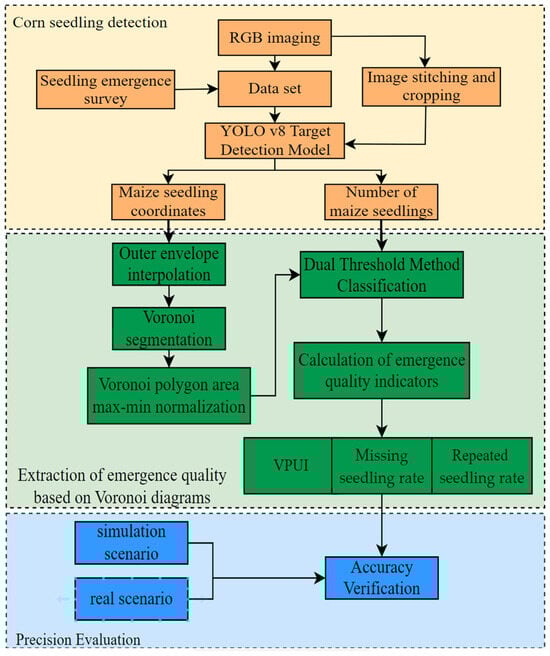
Figure 1.
Technical roadmap for evaluating maize seedling quality.
2.1. Study Site and Data Acquisition
The summer maize experiment in this study was conducted at the Xiaotangshan National Precision Agriculture Research and Demonstration Base in Changping District, Beijing (40°10′60″N, 116°26′30″E). The overview of the experimental area is shown in Figure 2. This region features flat terrain with an elevation of 41 to 53 m, an average annual precipitation of 508 mm, and an average annual temperature of 13 °C. As shown in Figure 2, the experiment used a completely randomized design to test five maize varieties (A1–A5). In 2022, 60 plots of 3.6 m × 3.6 m were planted and divided into four planting densities (90,000 plants/ha, 67,500 plants/ha, 60,000 plants/ha, 45,000 plants/ha), with three replicates for each density.
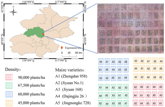
Figure 2.
Material plot overview map.
In this study, UAV aerial image data were collected on 8 June 2022 (maize V3 stage, cloudy) and 14 June 2022 (maize V5 stage, sunny) to obtain maize seedling images under different conditions and verify the target detection model’s adaptability to scene changes. The data were collected around 11 a.m. using a DJI Phantom 4 UAV (Shenzhen DJI Innovations Co., Ltd., Shenzhen, China) equipped with a 12-megapixel camera. The flight altitude was 10 m, and the flight speed was 2 m per second. The flight path was set with 80% forward overlap and 80% side overlap to facilitate image stitching. The image resolution was 5472 × 3648 pixels, stored in JPEG format. The camera exposure parameters, such as shutter speed (1/420 s), exposure mode, ISO, and white balance, were all set to automatic mode.
2.2. YOLO v8 Model to Extract the Number of Maize Seedlings and Their Location
The maize seedling imagery was stitched into orthophotos using DJI Terra v4.2 software, with a ground resolution of 0.013 m. The orthophotos were then cropped into a uniform size of 640 × 640 pixels to ensure model training efficiency. Images from different planting densities were randomly selected from the first and second batches of imagery data to create the training and test sets, enhancing the YOLO object detection model’s ability to recognize maize seedlings. The open-source image annotation tool LabelImg was used for manual annotation of the imagery data, with the annotations saved as txt files in YOLO format, including target class number, target bounding box center coordinates, and width–height ratio information. A total of 850 images were annotated, including 450 images from the maize V3 stage and 400 images from the maize V5 stage, providing sufficient training samples for model learning.
The YOLOv8 model stands out among many convolutional neural network models due to its high accuracy and computational efficiency. Compared to two-stage object detection models, YOLOv8 achieves similar or even higher accuracy with fewer computational resources. The network structure of YOLOv8 is shown in Figure 3. The backbone network adopts the C2f module, with the number of blocks in each stage changed from [3, 6, 9, 3] to [3, 6, 6, 3]. The most significant change is the replacement of Anchor Base with Anchor Free, drawing on the ideas from Task-Aligned One-Stage Object Detection (TOOD), You Only Look Once v6 (YOLO v6), and PaddlePaddle YOLO Enhanced (PP-YOLOE) [32]. This gives YOLOv8 excellent scalability, making it compatible with all previous versions of the YOLO framework, allowing for easy switching between different versions and performance comparisons.
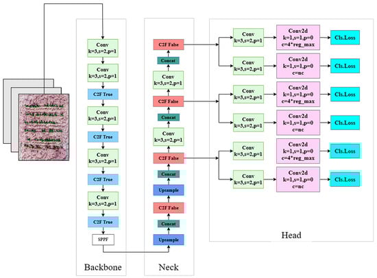
Figure 3.
Architecture of the YOLOv8 Model.
In this study, the annotated maize seedling dataset was randomly divided into training, validation, and test sets in a ratio of 8:1:1 to train the maize seedling object detection model. The hardware used in this study was a DELL XPS 17 2020 laptop (Dell Technologies, Round Rock, TX, USA), equipped with a 10th generation Intel Core i7-10750H processor, a NVIDIA GeForce RTX 2060 Max-Q graphics processor (6 GB GDDR6 VRAM), and 16 GB DDR4-2933MHz memory, running on the Windows 11 Professional operating system. The development environment was based on Python 3.7 and PyTorch 1.13.0 framework, with GPU acceleration enabled by CUDA 11.6 and cuDNN 11.5.50. During the training process, three image augmentation techniques—Gaussian blur, rotation, and flipping—were applied to the training set, expanding the dataset to six times its original size, reaching 5100 images. This was done to increase data diversity and improve the model’s generalization ability. The specific model training hyperparameters are shown in Table 1.

Table 1.
Training hyperparameters for the YOLOv8 model.
2.3. Computer Simulation of Maize Seedling Quantity and Position
In order to exclude the influence of the object detection model and to explore the accuracy of the Voronoi method in estimating the missing and repeated seedling rates, as well as the performance of the VPUI in representing spatial uniformity, this study designed four types of computer-generated coordinate point sets to simulate the distribution patterns of maize seedlings in the field. These patterns include a grid perturbation distribution (Figure 4B), a missing seedling only pattern (Figure 4C), a repeated seedling only pattern (Figure 4D), and a pattern with both missing and repeated seedlings. Different maize seedling distribution scenarios with varying uniformity, missing seedling rates, and repeated seedling rates were generated using these four distribution patterns. For each pattern and set of parameters, at least seven scenarios were simulated to ensure sufficient data.
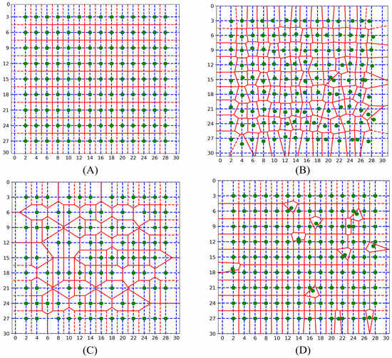
Figure 4.
Spatial distribution of maize seedlings under various simulation methods: (A) Simulation of absolute uniform spatial distribution of maize seedlings. (B) Simulation of spatial distribution of maize seedlings by the grid perturbation method, σ = 0.2. (C) Grid missing method to simulate the spatial distribution of maize seedlings, with missing proportion P1 = 0.3. (D) Grid repeating method to simulate the spatial distribution of maize seedlings, with repeating proportion of seedlings P2 = 0.06, and with an offset range of 0.3 times the plant spacing. The blue dashed lines represent a grid with a row-to-column spacing ratio of 2:3, the green dots represent the simulated maize positions, and the red solid lines are the Voronoi diagram with the green dots as control points.
Grid Perturbation Distribution (Figure 4B): A grid with a row-to-column spacing ratio of 2:3 is set, with the grid intersections (15 × 10 points) as the coordinates of maize seedlings. Subsequently, the coordinates of maize seedlings are given a normally distributed random perturbation with a mean of 0 and variable variance. The coordinates of maize seedlings under the grid perturbation distribution can be calculated using Equation (1).
In the above equation, (i, j) denotes the coordinates (row, column) of the maize seedlings. PD denotes the plant spacing, RD denotes the row spacing, and N(0, σ2) is the normal distribution. The randomness of the maize seedling distribution was adjusted according to the value of variance (σ2), with σ = 0 indicating the standard lattice distribution. The larger the σ value is, the higher the randomness of the maize seedling distribution.
Grid Missing Distribution (Figure 4C): A grid with a row-to-column spacing ratio of 2:3 is set, with the grid intersections (15 × 10 points) as the coordinates of maize seedlings. A certain proportion of maize seedlings (missing seedling proportion) is randomly removed to simulate the spatial distribution of maize seedlings with missing plants. The extent of missing plants is determined according to the missing seedling proportion P1 (P1 = 1%, 2%, …, 50%).
Grid Repeated Distribution (Figure 4D): A grid with a row-to-column spacing ratio of 2:3 is set, with the grid intersections (15 × 10 points) as the coordinates of maize seedlings. A certain proportion of additional maize seedlings (repeated seedling proportion) is randomly added near the existing maize coordinates (within a radius of 0.3 times the plant spacing) to simulate the spatial distribution of maize seedlings with repeats. The extent of repeats is determined according to the repeated seedling proportion P2 (P2 = 1%, 2%, …, 3%).
Combined Method for Missing and Repeated Seedlings: This method integrates methods 2 and 3 to generate simulated scenarios. In this study, method 3 was first used to randomly generate a scenario with a 10% repeated seedling rate. Then, based on this scenario, method 2 was applied to remove n% of points (excluding the repeated seedling points) to create multiple scenarios with both a 10% repeated seedling rate and an n% missing seedling rate. Alternatively, method 2 was used to randomly generate a scenario with a 10% missing seedling rate, and then method 3 was applied to add m% of points to create multiple scenarios with both a 10% missing seedling rate and an m% repeated seedling rate.
2.4. Extraction of Seedling Emergence Quality Indicators Based on Voronoi Diagrams
2.4.1. Optimization of the Voronoi Segmentation Algorithm Using the Outer Envelope Interpolation Method
This study uses Voronoi diagrams to analyze the spatial distribution of maize seedlings. To improve the accuracy of the analysis, we introduced an outer envelope interpolation method to optimize the edge effects of the Voronoi diagram and provided a detailed explanation of the Voronoi diagram construction process.
Data Preparation
We first extracted the coordinates of maize seedlings from the detection results of the YOLOv8 model. These coordinates can come from actual field images or simulated data generated for algorithm validation. Each coordinate point represents the position of a maize seedling in the image or simulated scenario.
Outer Envelope Interpolation Method
To address the issue of abnormally large polygons at the edges of the Voronoi diagram, we developed an outer envelope interpolation method. The specific steps of this method are as follows:
First, we determine the location coordinates of all maize seedlings (as shown in Figure 5A). Then, we use a Convex Hull algorithm to find the outer envelope polygon that contains all the maize seedling coordinate points (as shown in Figure 5B). Next, we expand this outer envelope polygon by increasing the average plant spacing and row spacing. Finally, we evenly insert additional points on the expanded polygon edge as outer envelope constraint points based on the average row and plant spacing of maize (as shown in Figure 5C).
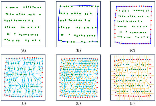
Figure 5.
Process of Voronoi diagram partitioning for the area occupied by maize seedlings: (A) Coordinates of maize seedlings. (B) Convex polygon containing all maize seedlings. (C) Expanded convex polygon with inserted virtual points. (D) Constructed Delaunay triangulation. (E) Circumcenters of each triangle calculated. (F) Voronoi diagram constructed by connecting all circumcenters. (Green dots represent maize seedlings, red dots are inserted virtual points, orange dots are circumcenters of triangles, blue dashed lines represent the Delaunay triangulation, the solid blue line represents the minimum convex polygon that includes all the maize seedlings, and orange solid lines represent the Voronoi diagram).
Voronoi Diagram Construction
After completing the outer envelope interpolation, we use the following steps to construct the Voronoi diagram:
First, we use the Lawson algorithm to perform Delaunay triangulation on all points (including maize seedling coordinates and interpolation points) as vertices (as shown in Figure 5D). Delaunay triangulation is a specific triangulation method that ensures that the circumcircle of any triangle in the mesh does not contain other points.
Then, we calculate the circumcenter of each Delaunay triangle (as shown in Figure 5E). The circumcircle is a circle that passes through the three vertices of the triangle, and its center can be calculated from the coordinates of the triangle’s vertices.
Finally, we form the boundaries of the Voronoi polygons by connecting the circumcenters of adjacent triangles with shared edges (as shown in Figure 5F). For the outermost triangles, we calculate the perpendicular bisectors of their edges and extend them as the external boundary of the Voronoi diagram.
Implementation Details
We used the Python programming language and its scientific computing libraries to implement the above algorithms. Specifically, we utilized the spatial algorithm module in the SciPy library for Delaunay triangulation and Voronoi diagram generation. To visualize the results, we used the Matplotlib library.
2.4.2. Calculation of Indicators for Evaluation of Emergence Quality
- (1)
- VPUI
This study uses the coefficient of variation (CV) to construct the Voronoi Polygon Uniformity Index (VPUI), as CV is a dimensionless statistic that effectively reflects the dispersion degree of data values and is not affected by planting density [33]. The specific calculation formulas for VPUI are shown in Equations (2)–(5).
where CV is the coefficient of variation, σ is the standard deviation of the areas of all Voronoi cells, is the area of the Voronoi cell corresponding to the ith maize seedling, is the number of maize seedlings, FP is the average area of the Voronoi diagram, and VPUI is the Voronoi Polygon Uniformity Index.
- (2)
- Missing Seedling Rate and Repeated Seeding Rate
Firstly, Equation (6) is used to normalize the area data of all Voronoi cells of all plots with maximum–minimum values, and the area values of different magnitudes are uniformly mapped into the interval [0, 1]. This approach helps to place the Voronoi polygons from fields with different planting densities on the same level for comparison, making this method applicable for analyzing various planting densities.
where is the area of the Voronoi cell corresponding to the ith maize seedling, is the minimum area of all Voronoi polygon samples, is the maximum area of all Voronoi polygon samples, and is the maximum–minimum normalized Voronoi area.
In the case of missing seedlings, the adjacent two Voronoi polygons will be larger than in normal conditions, and in the case of repeated seedlings, the adjacent two Voronoi polygons will be smaller than in normal conditions. In real scenarios, there are cases where missing seedlings are followed by repeated seedlings. In such instances, the area of the Voronoi polygon for repeated seedlings is not affected, while the area of the Voronoi polygon for missing seedlings may slightly decrease. However, this decrease is negligible compared to the difference in area between the Voronoi polygons for missing, normal, and repeated seedlings. Therefore, the value of can be used to determine whether there are missing or repeated seedlings. Larger Voronoi polygons are considered to contain un-emerged maize seed planting spots, while smaller Voronoi polygons are considered to contain repeated maize seedlings. Specifically, the Voronoi cells are classified into three categories based on the value of : normal cells, missing seedling cells, and repeated seedling cells. If , it is a missing seedling cell; if, it is a repeated seedling cell; and if , it is a normal cell. The thresholds and are set based on the distribution measured from the images. In this study, four plots were randomly selected from each of the four planting densities (90,000, 67,500, 60,000, and 45,000 plants/ha), resulting in a total of 2096 Voronoi polygon areas. The optimal classification thresholds were determined based on grid search, with set at 0.26 and set at 0.68.
Through the above classification, the Voronoi cells in the target area can be divided into three categories: missing seedling cells, repeated seedling cells, and normal cells. Based on the classification results, the missing seedling rate and repeated seedling rate in the target area can be calculated using Equations (7)–(9):
where MSR is the seedling deficiency rate, RSR is the reseeding rate, is the number of Voronoi polygons in the target area, is the number of maize plants in the ideal situation (no seedling deficiency and no reseeding), is the number of normal Voronoi cells, is the maximum–minimum normalized Voronoi area, is the area of the ith normal Voronoi cell, and r is the reseeding number of Voronoi cells.
2.5. Evaluation Indicators
2.5.1. YOLO v8 Evaluation Indicators
This study evaluates the performance of the YOLO v8 model using four indicators: precision, recall, F1 score, and mean average precision. The specific calculation formulas for these indicators are shown in Equations (10)–(14) [34].
where is the number of detected maize seedlings that are real maize seedlings, is the number of real maize seedlings missed out from the detection, is the number of maize seedlings incorrectly detected as maize seedlings, and is the true number.
2.5.2. Missing Seedling Rate and Repeated Seedling Rate Evaluation Indicators
The number of missing and repeated seedlings in the experimental plots was recorded through manual visual inspection of the drone images and the actual missing seedling rate and repeated seedling rate were calculated using Equations (15) and (16) [35].
where is the number of missing seedlings, is the number of maize seedlings, and is the number of re-seedlings.
This study uses RMSE and R2 to evaluate the accuracy of the Voronoi method for estimating the missing seedling rate and repeated seedling rate. The formulas are shown in Equations (17) and (18) [36].
where is the true value, is the predicted value, is the mean of the true value, and is the sample size.
3. Results
3.1. YOLOv8 Object Detection Model Performance
3.1.1. Training Accuracy
As shown in Table 2, the YOLO v8 model achieved the highest scores in precision, recall, F1 score, and mAP@0.5 when compared horizontally with the two typical object detection models: YOLO v5 and Faster R-CNN. In Figure 6, the F1–confidence curve and precision–recall curve for each object detection model are shown. It can be seen from the figure that the YOLO v8 model achieved the highest F1 score and had better precision at all recall rates compared to the other two models. In summary, the YOLO v8 model achieved the best training accuracy on the custom dataset used in this study.
Table 2.
Performance comparison of different maize seedling detection models.
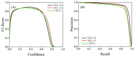
Figure 6.
F1 score versus confidence and precision–recall curves for different models: (A) F1 score versus confidence curves. (B) Precision–recall curves.
3.1.2. Detection Performance of the YOLO v8 Model in Different Scenarios
Based on Equation (14), the detection accuracy of each model for each image can be calculated. The detection results are shown in Table 3. From the table, it can be seen that the YOLO v8 model achieved the highest accuracy in detecting images in both scenarios, with an optimal accuracy of 98.2% for detecting images of maize plots at the V3 stage under cloudy conditions.
Table 3.
Detection accuracy of each model under different weather conditions.
Although all object detection models achieved higher accuracy for detecting images of maize plots at the V3 stage under cloudy conditions, the difference in detection accuracy for images in the V3 and V5 stages varies among the models. The maize seedling detection results of the YOLO v8 model are shown in Figure 7. The detection accuracy of the YOLO v8 model for images of maize plots at the V5 stage under sunny conditions was only 2.8% lower than that for images at the V3 stage under cloudy conditions, while the accuracy of the YOLO v5 model and Faster R-CNN model decreased by 5.6% and 7.1%, respectively. The reason for the differences in detection accuracy among the models in the two scenarios is that the V5 stage maize seedlings have more leaves and larger leaf areas, leading to an increase in seedling overlap, and the ground shadows under sunny conditions add further interference. The YOLO v8 model had the smallest difference in detection accuracy between the two scenarios, demonstrating its good adaptability to high overlap rates and strong shadow scenes.
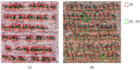
Figure 7.
YOLO v8_s model maize seedling detection results: (A) Detection results for maize seedlings at the V3 stage under cloudy conditions. (B) Detection results for maize seedlings at the V5 stage under sunny conditions.
3.2. Voronoi Method for Extracting Seedling Quality Indicators in Simulated Maize Plots
3.2.1. Validation of the Reasonableness of the Maize Seedling VPUI Evaluation Indicator
Figure 8 shows the distribution of the coefficients of variation for the area of the Voronoi diagram and plant spacing in the simulated distribution of maize. As can be seen from the figure, both coefficients effectively characterize the uniformity of spatial distribution. In absolutely uniform conditions, their values are zero. As the degree of non-uniformity increases, both the coefficient of variation of the Voronoi diagram area and the coefficient of variation of plant spacing show an upward trend, with the growth rate gradually decreasing. However, compared to the coefficient of variation of plant spacing, the coefficient of variation of the Voronoi diagram area is more concentrated and shows a more stable change trend. For indices describing seedling quality, the coefficient of variation of the Voronoi diagram area undoubtedly has superior performance. Therefore, the VPUI calculated based on the coefficient of variation of the Voronoi diagram area can effectively represent the uniformity of the spatial distribution of maize seedlings.
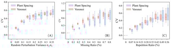
Figure 8.
Changes in the CV of the maize seedling Voronoi diagram and plant spacing under different simulation methods: (A) The change trend of CV with increasing , . (B) The change trend of CV with an increasing missing rate. (C) The change trend of CV with an increasing duplication rate.
3.2.2. Estimation Accuracy of Missing and Repeated Seedling Rates in Simulated Scenarios
Based on methods 2, 3, and 4 in Section 2.3, four different types of scenarios with varying rates of missing and repeated seedlings were simulated. As shown in Figure 9, the Voronoi method provides very reliable estimates when the missing and repeated seedling rates range from 0 to 56%. In scenarios with only missing seedlings (Figure 9A), the estimation accuracy of the missing seedling rate using the Voronoi method is very high, with a RMSE and R2 of 2.127 and 0.927, respectively. In scenarios with only repeated seedlings (Figure 9B), the RMSE and R2 for estimating the repeated seedling rate are 3.462 and 0.815. In single scenarios with either missing or repeated seedlings, the accuracy of the Voronoi method for estimating the missing seedling rate remains very stable. However, when the repeated seedling rate exceeds 30%, the Voronoi method tends to overestimate the repeated seedling rate.
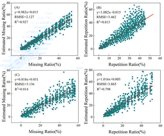
Figure 9.
Scatter plots of the Voronoi method estimates versus simulated values. (A) Missing seedling rate. (B) Repeated seedling rate. (C) Missing seedling rate scatter plot when both missing and repeated seedlings are present, with a 10% repeated seedling rate. (D) Repeated seedling rate scatter plot when both missing and repeated seedlings are present, with a 10% missing seedling rate.
In complex scenarios with both missing and repeated seedlings, with a background of a 10% repeated seedling rate (Figure 9C), the estimation accuracy of the missing seedling rate by the Voronoi method decreases, with a RMSE and R2 of 3.316 and 0.814. With a background of a 10% missing seedling rate (Figure 9D), the RMSE and R2 for estimating the repeated seedling rate are 3.865 and 0.798. Compared to single scenarios with only missing or only repeated seedlings, scenarios with both missing and repeated seedlings are more complex. For the estimation of the missing seedling rate, the estimation value tends to decrease as the missing seedling rate increases, resulting in a significant reduction in the overall estimation accuracy. For the estimation of the repeated seedling rate, the tendency to overestimate when the rate exceeds 30% also occurs, with a slight overall decrease in estimation accuracy.
3.3. Voronoi Method for Extracting Seedling Quality Indicators in Real Scenarios
3.3.1. Estimation Accuracy of Missing and Repeated Seedling Rates
In simulated scenarios, the Voronoi method achieved high accuracy in estimating missing and repeated seedling rates. However, real scenarios are more complex, and the estimation results are influenced by the detection accuracy of the target detection model. To evaluate the accuracy of the Voronoi method in real scenarios, this study uses the missing and repeated seedling rates estimated by manual visual inspection as the true values to analyze the estimation accuracy of the Voronoi method and compares the results with the traditional plant spacing method. The plant spacing method calculates the theoretical number of seedlings in the entire field using the average plant spacing and row spacing, and the missing and repeated seedling rates can be calculated using Equation (19).
where represents the theoretical number of maize seedlings in a plot, and represents the actual number of maize seedlings. If < , it is considered that there are missing maize seedlings, and p is the missing seedling rate; if > , it is considered that there are repeated maize seedlings, and p is the repeated seedling rate.
Figure 9 shows scatter plots of the estimated values versus the true values for the missing seedling rate and repeated seedling rate using the Voronoi method and the plant spacing method in a real-world scenario. It can be seen that the accuracy of the Voronoi method in estimating missing seedling rates and repeated seedling rates is significantly improved compared to the plant spacing method. From Figure 10A, the R2 value for the missing seedling rate estimated by the Voronoi method is 0.773, with a RMSE of 3.9, which is an improvement of 0.09 in R2 compared to the plant spacing method (Figure 10C). From Figure 10B, the R2 value for the repeated seedling rate estimated by the Voronoi method is 0.94, with a RMSE of 1.2, which is an improvement of 0.544 in R2 compared to the plant spacing method (Figure 10D).
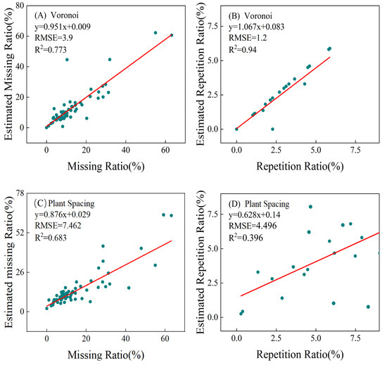
Figure 10.
Scatter plots of estimated missing and multiple seedling rates from different methods versus ground truth values. (A) Scatter plot of missing rates estimated by the Voronoi method versus ground truth. (B) Scatter plot of multiple seedling rates estimated by the Voronoi method versus ground truth. (C) Scatter plot of missing rates estimated by the plant spacing method versus ground truth. (D) Scatter plot of multiple seedling rates estimated by the plant spacing method versus ground truth.
3.3.2. Maize Seedling Quality Distribution Map
As shown in Figure 11, this study successfully extracted the maize seedling quality of 60 plots at the V3 stage using the Voronoi method. Figure 11A presents the heat map of the missing seedling rate distribution. We can observe that the missing seedling rates in most plots range between 20% and 50%, with significant variations among different plots and varieties. Jiyuan 168 exhibited the highest average missing seedling rate at 42.52%, while Dajingjiu 26 had the lowest at 29.87%. Figure 11B illustrates the heat map of the repeated seedling rate distribution. Jingnongke 728 showed the highest average repeated seedling rate at 10.33%, whereas Zhengdan 958 had the lowest among the five varieties at 3.74%. Figure 11C displays the heat map of uniformity distribution. Dajingjiu 26 demonstrated the highest average VPUI at 0.84, while Jiyuan 168 had the lowest among the five varieties at 0.72. Consequently, Dajingjiu 26 was determined to be the variety with the best seedling quality.
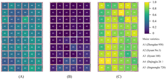
Figure 11.
Heat maps of seedling quality. (A) Missing seedling rate. (B) Repeated seedling rate. (C) VPUI. (Values in (A,B) should be multiplied by 100% when reading).
3.4. The Impact of Edge Expansion Effect on Voronoi Spatial Analysis
For maize planting plots with fragmented shapes or small areas, as well as breeding plots, the edge expansion effect significantly impacts the estimation accuracy. Taking the small area experimental plots as an example, when using the Voronoi method to estimate the missing seedling rate and repeated seedling rate of maize experimental plots, the classification results without optimization (Figure 12A) show that Voronoi polygons at the edges are mistakenly identified as missing seedlings, compared to the Voronoi classification results processed with external envelope interpolation (Figure 12B).
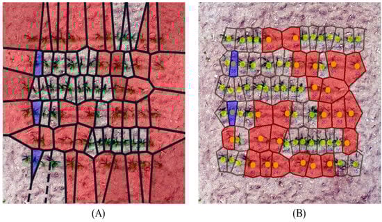
Figure 12.
Classification results of Voronoi polygons. (A) Classification results without virtual points added. (B) Classification results with virtual points added. (Red Voronoi units represent missing seedlings, uncolored Voronoi units represent normal units, and blue Voronoi units represent multiple seedlings).
Figure 13 illustrates the accuracy of estimating the missing seedling rate and repeated seedling rate using the Voronoi method without outer envelope interpolation. Figure 13A shows that the R2 between the estimated and actual missing seedling rates is 0.568, with a RMSE of 11.6. Figure 13B indicates that the R2 between the estimated and actual repeated seedling rates is 0.89, with a RMSE of 1.483. This demonstrates that the edge expansion effect reduced the coefficient of determination (R2) for the missing seedling rate estimation by 0.205 and for the repeated seedling rate estimation by 0.05. These results prove that, for small, fragmented plots and breeding blocks, the outer envelope interpolation method can effectively limit the abnormal increase in area of Voronoi units at the edges and improve the estimation accuracy of the missing seedling rate and repeated seedling rate.
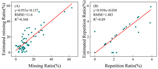
Figure 13.
Scatter plots of the missing and multiple seedling rates estimated by the Voronoi method without virtual points versus ground truth values. (A) Scatter plot of the predicted missing rates versus ground truth missing rates. (B) Scatter plot of the predicted multiple seedling rates versus ground truth multiple seedling rates.
4. Discussion
The method proposed in this study for evaluating the seedling quality based on Voronoi diagrams includes three indicators: VPUI, missing seedling rate, and repeated seedling rate. In the computer model scenarios, VPUI demonstrated superior performance as an evaluation indicator (Figure 8). Furthermore, VPUI has a significant potential advantage in that it can also characterize intraspecific competition. Voronoi diagrams are graphical representations describing the distribution of control or influence of points over their own areas [37,38]. Based on the maize seedling coordinates detected by YOLOv8, Voronoi segmentation of the maize field results in Voronoi polygons that represent the growth space of each maize plant. Larger Voronoi areas indicate that the maize plant can utilize more surrounding resources for growth and development [5,39]. Therefore, under the same planting density, a higher uniformity (VPUI) indicates more even resource distribution and less intraspecific competition within the maize population. Conversely, lower uniformity suggests uneven resource distribution and greater intraspecific competition within the maize population.
The Voronoi method achieved high accuracy in estimating missing and repeated seedling rates in both simulated scenarios (Figure 9) and real-world scenarios (Figure 10A,B). However, when comparing the two, we found differences in the estimation accuracy between the simulated and real-world scenarios. For the missing seedling rates, the estimation accuracy is highest in the scenario with only missing seedlings (Figure 9A), followed by the scenario with both missing and repeated seedlings (Figure 9C), and lowest in the real-world scenario (Figure 10A). The scenario with both missing and repeated seedlings is quite complex, which affects the accuracy of the Voronoi method. Additionally, the accuracy of the object detection model is also a factor influencing the final estimation accuracy, contributing to the lower accuracy of missing seedling rate estimates in the real-world scenario (Figure 10A) compared to the simulated scenarios. For the repeated seedling rate, the accuracy differs only slightly between the scenario with only repeated seedlings (Figure 9B) and the scenario with both missing and repeated seedlings (Figure 9D), indicating that the presence of both missing and repeated seedlings does not significantly impact the accuracy of the Voronoi method for estimating the repeated seedling rate. From Figure 9B,D, it is evident that the Voronoi method has higher estimation accuracy in scenarios with lower actual repeated seedling rates. Since the actual repeated seedling rates in the real-world scenario (Figure 10B) are all below 10%, the accuracy in the real-world scenario is even higher than in the simulated scenarios. Data quantity and distribution are also important factors affecting accuracy.
Moreover, in practical applications, many factors affect the extraction of seedling quality using the Voronoi method, such as the accuracy of target detection and the timing of image acquisition. The VPUI, missing seedling rate, and repeated seedling rate are all derived from further analysis based on the maize seedling detection results. Table 3 shows that the YOLO v8 model demonstrates high detection accuracy for maize seedlings. However, as the overlap between maize seedlings increases and shadows interfere, the detection accuracy of sunny V5 stage images is lower than that of cloudy V3 stage images. Therefore, acquiring high-quality maize seedling images with low leaf overlap and minimal shadows, as well as optimizing the network structure of target detection models to enhance their resistance to maize overlap and image shadows, are crucial means to improve maize seedling detection accuracy [32,40].
Image acquisition timing also significantly impacts missing and repeated seedling rates. In actual crop growth processes, differences in planting viability, sowing depth, and soil conditions lead to variations in seedling emergence times. These temporal differences result in dynamic changes of extracted VPUI, missing seedling rate, and repeated seedling rate indicators over time [41,42]. Table 4 illustrates the changes in seedling quality indicators for 60 plots from the V3 to V5 stages. The average missing seedling rate extracted from V3 stage maize seedling images reached 35.6%, decreasing to 9.16% at the V5 stage. The YOLO v8 target detection model’s accuracy for these two stages differed by only 2.8%. Comparison of the V3 and V5 stage images revealed that many maize seeds had not yet emerged at the V3 stage, indicating that inconsistent emergence times was the primary cause of the significant difference in the missing seedling rates between the two stages. Therefore, to comprehensively evaluate crop seedling quality, multiple observations throughout the entire emergence stage are necessary, rather than being limited to a specific time point.
Table 4.
Quality index table extracted by the Voronoi method at different growth stages.
The seedling quality evaluation method based on UAV remote sensing imagery and Voronoi spatial analysis has broad application prospects, not only for maize crops but also for other row-planted crops such as cotton and soybeans. This method integrates UAV remote sensing, computer vision, and spatial analysis technologies, constructing a seedling quality evaluation index system and a complete technical process based on maize seedling spatial positions. It provides an alternative technical solution for field managers and breeders to quickly understand maize seedling quality.
5. Conclusions
This study utilized high-resolution drone imagery to capture maize seedlings and developed a seedling quality evaluation method based on a deep learning object detection algorithm and Voronoi spatial analysis. The method includes three key indicators: Voronoi Polygon Uniformity Index (VPUI), missing seedling rate, and repeated seedling rate. The effectiveness of this method was validated by comparing it with the traditional plant spacing analysis method. The main conclusions are as follows:
- This study successfully detected maize seedlings in the field using the YOLO v8 deep learning object detection model, achieving an accuracy of over 95%. Compared to the YOLO v5 model and Faster_RCNN model, YOLO v8 demonstrated better adaptability to occlusion and shadows, effectively identifying maize seedlings under complex conditions.
- The study successfully extracted the VPUI, missing seedling rate, and repeated seedling rate from the Voronoi diagram of the maize field. Compared to using plant spacing information, the Voronoi diagram-based spatial analysis method for calculating VPUI has greater biological significance. Additionally, the Voronoi-based estimation of the missing seedling rate and repeated seedling rate showed higher accuracy, with a R2 of 0.773 for the missing seedling rate and 0.94 for the repeated seedling rate.
- For fragmented plots or maize breeding plots, the Convex Hull interpolation method effectively constrained the shape of the edge Voronoi polygons, improving the accuracy of the missing seedling rate estimation. In this study’s experimental plots, the R2 of the missing seedling rate increased by 0.21 after processing.
Author Contributions
Conceptualization, H.Y., G.Y. and C.L.; methodology, L.R., H.Y. and C.L.; validation, L.R. and H.Y.; formal analysis, L.R. and H.Y.; performed experiments, L.R., Z.C., D.Z., C.Z., B.X., H.F., L.R. and Z.L.; Conceptualization, H.Y., G.Y. and C.L.; data curation, Z.C. and D.Z.; writing—original draft preparation, L.R., C.L. and H.Y; writing—review and editing, H.Y., D.Z. and L.R. All authors have read and agreed to the published version of the manuscript.
Funding
This research was supported by the National Key Research and Development Program (2023YFD2000104 and 2021YFD2000102), the National Natural Science Foundation of China (42371373), the Beijing Academy of Agriculture and Forestry Sciences Special Fund for Technological Innovation Capacity Building (KJCX20230434), the Henan Provincial Natural Science Foundation (242300420221), and the Henan Polytechnic University National Major Scientific Research Achievement Cultivation Fund (NSFRF240101).
Data Availability Statement
All data from this paper are available upon contact with the corresponding author Hao Yang via email at yangh@nercita.org.cn.
Conflicts of Interest
The authors declare no conflicts of interest.
References
- Citations: Exploring Climate Change Resilience of Major Crops in Somalia: Implications for Ensuring Food Security. Available online: https://www.tandfonline.com/doi/citedby/10.1080/14735903.2024.2338030?scroll=top&needAccess=true (accessed on 5 July 2024).
- Plant Emergence and Maize (Zea mays L.) Yield across Multiple Farmers’ Fields|Semantic Scholar. Available online: https://www.semanticscholar.org/paper/Plant-emergence-and-maize-(Zea-mays-L.)-yield-Albarenque-Basso/72d31cf3de6a67ead11155252c528dfc14631522 (accessed on 8 May 2024).
- Karayel, D.; Özmerzi, A. Evaluation of Three Depth-Control Components on Seed Placement Accuracy and Emergence for a Precision Planter. Appl. Eng. Agric. 2008, 24, 271–276. [Google Scholar] [CrossRef]
- Shah, A.N.; Tanveer, M.; Abbas, A.; Yildirim, M.; Shah, A.A.; Song, Y. Combating Dual Challenges in Maize Under High Planting Density: Stem Lodging and Kernel Abortion. Front. Plant Sci. 2021, 12, 699085. [Google Scholar] [CrossRef]
- Zhai, L.; Xie, R.; Ming, B.; Li, S.; Ma, D. Evaluation and Analysis of Intraspecific Competition in Maize: A Case Study on Plant Density Experiment. J. Integr. Agric. 2018, 17, 2235–2244. [Google Scholar] [CrossRef]
- Shirzadifar, A.; Maharlooei, M.; Bajwa, S.G.; Oduor, P.G.; Nowatzki, J.F. Mapping Crop Stand Count and Planting Uniformity Using High Resolution Imagery in a Maize Crop. Biosyst. Eng. 2020, 200, 377–390. [Google Scholar] [CrossRef]
- Feng, A.; Zhou, J.; Vories, E.; Sudduth, K.A. Evaluation of Cotton Emergence Using UAV-Based Narrow-Band Spectral Imagery with Customized Image Alignment and Stitching Algorithms. Remote Sens. 2020, 12, 1764. [Google Scholar] [CrossRef]
- Liu, M.; Su, W.-H.; Wang, X.-Q. Quantitative Evaluation of Maize Emergence Using UAV Imagery and Deep Learning. Remote Sens. 2023, 15, 1979. [Google Scholar] [CrossRef]
- Feng, H.; Tao, H.; Li, Z.; Yang, G.; Zhao, C. Comparison of UAV RGB Imagery and Hyperspectral Remote-Sensing Data for Monitoring Winter Wheat Growth. Remote Sens. 2022, 14, 3811. Available online: https://www.mdpi.com/2072-4292/14/15/3811 (accessed on 5 July 2024). [CrossRef]
- Gao, M.; Yang, F.; Wei, H.; Liu, X. Automatic Monitoring of Maize Seedling Growth Using Unmanned Aerial Vehicle-Based RGB Imagery. Remote Sens. 2023, 15, 3671. [Google Scholar] [CrossRef]
- Weiss, M.; Baret, F. Using 3D Point Clouds Derived from UAV RGB Imagery to Describe Vineyard 3D Macro-Structure. Remote Sens. 2017, 9, 111. [Google Scholar] [CrossRef]
- Yang, Y.; Li, Q.; Mu, Y.; Li, H.; Wang, H.; Ninomiya, S.; Jiang, D. UAV-Assisted Dynamic Monitoring of Wheat Uniformity toward Yield and Biomass Estimation. Plant Phenomics 2024, 6, 0191. [Google Scholar] [CrossRef]
- Pimstein, A.; Karnieli, A.; Bonfil, D.J. Wheat and Maize Monitoring Based on Ground Spectral Measurements and Multivariate Data Analysis. J. Appl. Remote Sens. 2007, 1, 013530. [Google Scholar]
- Xiao, J.; Suab, S.A.; Chen, X.; Singh, C.K.; Singh, D.; Aggarwal, A.K.; Korom, A.; Widyatmanti, W.; Mollah, T.H.; Minh, H.V.T.; et al. Enhancing Assessment of Maize Growth Performance Using Unmanned Aerial Vehicles (UAVs) and Deep Learning. Measurement 2023, 214, 112764. [Google Scholar] [CrossRef]
- Vong, C.N.; Conway, L.S.; Feng, A.; Zhou, J.; Kitchen, N.R.; Sudduth, K.A. Maize Emergence Uniformity Estimation and Mapping Using UAV Imagery and Deep Learning. Comput. Electron. Agric. 2022, 198, 107008. [Google Scholar] [CrossRef]
- Li, B.; Xu, X.; Han, J.; Zhang, L.; Bian, C.; Jin, L.; Liu, J. The Estimation of Crop Emergence in Potatoes by UAV RGB Imagery. Plant Methods 2019, 15, 15. [Google Scholar] [CrossRef]
- Pang, Y.; Shi, Y.; Gao, S.; Jiang, F.; Veeranampalayam-Sivakumar, A.-N.; Thompson, L.; Luck, J.; Liu, C. Improved Crop Row Detection with Deep Neural Network for Early-Season Maize Stand Count in UAV Imagery. Comput. Electron. Agric. 2020, 178, 105766. [Google Scholar] [CrossRef]
- Quick and Accurate Monitoring Peanut Seedlings Emergence Rate through UAV Video and Deep Learning|Semantic Scholar. Available online: https://www.semanticscholar.org/paper/Quick-and-accurate-monitoring-peanut-seedlings-rate-Lin-Chen/efec36a86e07143737eba08db6395dde3139b4ea (accessed on 8 May 2024).
- Gao, X.; Zan, X.; Yang, S.; Zhang, R.; Chen, S.; Zhang, X.; Liu, Z.; Ma, Y.; Zhao, Y.; Li, S. Maize Seedling Information Extraction from UAV Images Based on Semi-Automatic Sample Generation and Mask R-CNN Model. Eur. J. Agron. 2023, 147, 126845. [Google Scholar] [CrossRef]
- Yang, T.; Zhu, S.; Zhang, W.; Zhao, Y.; Song, X.; Yang, G.; Yao, Z.; Wu, W.; Liu, T.; Sun, C.; et al. Unmanned Aerial Vehicle-Scale Weed Segmentation Method Based on Image Analysis Technology for Enhanced Accuracy of Maize Seedling Counting. Agriculture 2024, 14, 175. [Google Scholar] [CrossRef]
- Tollenaar, M.; Deen, W.; Echarte, L.; Liu, W. Effect of Crowding Stress on Dry Matter Accumulation and Harvest Index in Maize. Agron. J. 2006, 98, 930–937. [Google Scholar] [CrossRef]
- Valente, J.; Sari, B.; Kooistra, L.; Kramer, H.; Mücher, S. Automated Crop Plant Counting from Very High-Resolution Aerial Imagery. Precis. Agric. 2020, 21, 1366–1384. [Google Scholar] [CrossRef]
- Ren, C.; Kim, D.-K.; Jeong, D. A Survey of Deep Learning in Agriculture: Techniques and Their Applications. J. Inf. Process. Syst. 2020, 16, 1015–1033. [Google Scholar] [CrossRef]
- Li, X.; Krishnamurthy, A.; Hanniel, I.; McMains, S. Edge Topology Construction of Voronoi Diagrams of Spheres in Non-General Position. Comput. Graph. 2019, 82, 332–342. [Google Scholar] [CrossRef]
- Beard, K.; Kimble, M.; Yuan, J.; Evans, K.S.; Liu, W.; Brady, D.; Moore, S. A Method for Heterogeneous Spatio-Temporal Data Integration in Support of Marine Aquaculture Site Selection. J. Mar. Sci. Eng. 2020, 8, 96. [Google Scholar] [CrossRef]
- Liu, S.; Song, M.; Chen, S.; Fu, X.; Zheng, S.; Hu, W.; Gao, S.; Cheng, K. An Intelligent Modeling Framework to Optimize the Spatial Layout of Ocean Moored Buoy Observing Networks. Front. Mar. Sci. 2023, 10, 1134418. [Google Scholar] [CrossRef]
- Xue, H.; Kurokawa, M.; Ying, B.-W. Correlation between the Spatial Distribution and Colony Size Was Common for Monogenetic Bacteria in Laboratory Conditions. BMC Microbiol. 2021, 21, 114. [Google Scholar] [CrossRef]
- Laporte, G.; Mesa, J.A.; Ortega, F.A.; Pozo, M.A. Locating a Metro Line in a Historical City Centre: Application to Sevilla. J. Oper. Res. Soc. 2009, 60, 1462–1466. [Google Scholar] [CrossRef]
- Zhang, H.; Tian, T.; Feng, O.; Wu, S.; Zhong, G. Research on Public Air Route Network Planning of Urban Low-Altitude Logistics Unmanned Aerial Vehicles. Sustainability 2023, 15, 12021. [Google Scholar] [CrossRef]
- Karayel, D. Evaluation of Seed Distribution in the Horizontal Plane and Plant Growing Area for Row Seeding Using Voronoi Polygons. J. Agric. Sci.-Tarim Bilim. Derg. 2010, 16, 97–103. [Google Scholar]
- Wang, X.; Tang, Q.; Chen, Z.; Luo, Y.; Fu, H.; Li, X. Estimating and Evaluating the Rice Cluster Distribution Uniformity with UAV-Based Images. Sci. Rep. 2021, 11, 21442. [Google Scholar] [CrossRef]
- Mota-Delfin, C.; de J. López-Canteñs, G.; López-Cruz, I.L., I.L.; Romantchik-Kriuchkova, E.; Olguín-Rojas, J.C. Detection and Counting of Maize Plants in the Presence of Weeds with Convolutional Neural Networks. Remote Sens. 2022, 14, 4892. [Google Scholar] [CrossRef]
- Bootstrap Confidence Intervals for the Coefficient of Quartile Variation: Communications in Statistics—Simulation and Computation: Vol 48, No 7—Get Access. Available online: https://www.tandfonline.com/doi/full/10.1080/03610918.2018.1435800 (accessed on 5 July 2024).
- Gao, K.; Liu, B.; Yu, X.; Qin, J.; Zhang, P.; Tan, X. Deep Relation Network for Hyperspectral Image Few-Shot Classification. Remote Sens. 2020, 12, 923. Available online: https://www.mdpi.com/2072-4292/12/6/923 (accessed on 5 July 2024). [CrossRef]
- Cui, J.; Zheng, H.; Zeng, Z.; Yang, Y.; Ma, R.; Tian, Y.; Tan, J.; Feng, X.; Qi, L. Real-Time Missing Seedling Counting in Paddy Fields Based on Lightweight Network and Tracking-by-Detection Algorithm. Comput. Electron. Agric. 2023, 212, 108045. [Google Scholar] [CrossRef]
- Chen, P.; Wang, F. New Textural Indicators for Assessing Above-Ground Cotton Biomass Extracted from Optical Imagery Obtained via Unmanned Aerial Vehicle. Remote Sens. 2020, 12, 4170. Available online: https://www.mdpi.com/2072-4292/12/24/4170 (accessed on 5 July 2024). [CrossRef]
- Au, C.K. Spatial and Temporal Competition as a Two Dimensional Kinetic Voronoi Diagram. Comput.-Aided Des. 2008, 40, 139–149. [Google Scholar] [CrossRef]
- Liao, J.; Li, Z.; Quets, J.J.; Nijs, I. Effects of Space Partitioning in a Plant Species Diversity Model. Ecol. Model. 2013, 251, 271–278. [Google Scholar] [CrossRef]
- Hussain, Z.; Marwat, K.B.; Cardina, J.; Khan, I.A. Xanthium strumarium L. Impact on Maize Yield and Yield Components. Turk. J. Agric. For. 2014, 38, 39–46. [Google Scholar] [CrossRef]
- Wang, B.; Yang, G.; Yang, H.; Gu, J.; Xu, S.; Zhao, D.; Xu, B. Multiscale Maize Tassel Identification Based on Improved RetinaNet Model and UAV Images. Remote Sens. 2023, 15, 2530. Available online: https://www.mdpi.com/2072-4292/15/10/2530 (accessed on 5 July 2024). [CrossRef]
- (PDF) Influence of Planter Downforce Setting and Ground Speed on Seeding Depth and Plant Spacing Uniformity of Maize. Available online: https://www.researchgate.net/publication/336749838_Influence_of_Planter_Downforce_Setting_and_Ground_Speed_on_Seeding_Depth_and_Plant_Spacing_Uniformity_of_Maize (accessed on 5 July 2024).
- Planting Depth Affects Maize Emergence, Growth and Development, and Yield|Agronomy Journal. Available online: https://acsess.onlinelibrary.wiley.com/doi/full/10.1002/agj2.20701 (accessed on 5 July 2024).
Disclaimer/Publisher’s Note: The statements, opinions and data contained in all publications are solely those of the individual author(s) and contributor(s) and not of MDPI and/or the editor(s). MDPI and/or the editor(s) disclaim responsibility for any injury to people or property resulting from any ideas, methods, instructions or products referred to in the content. |
© 2024 by the authors. Licensee MDPI, Basel, Switzerland. This article is an open access article distributed under the terms and conditions of the Creative Commons Attribution (CC BY) license (https://creativecommons.org/licenses/by/4.0/).