
InSAR Integrated Machine Learning Approach for Landslide Susceptibility Mapping in California


Abstract
:1. Introduction
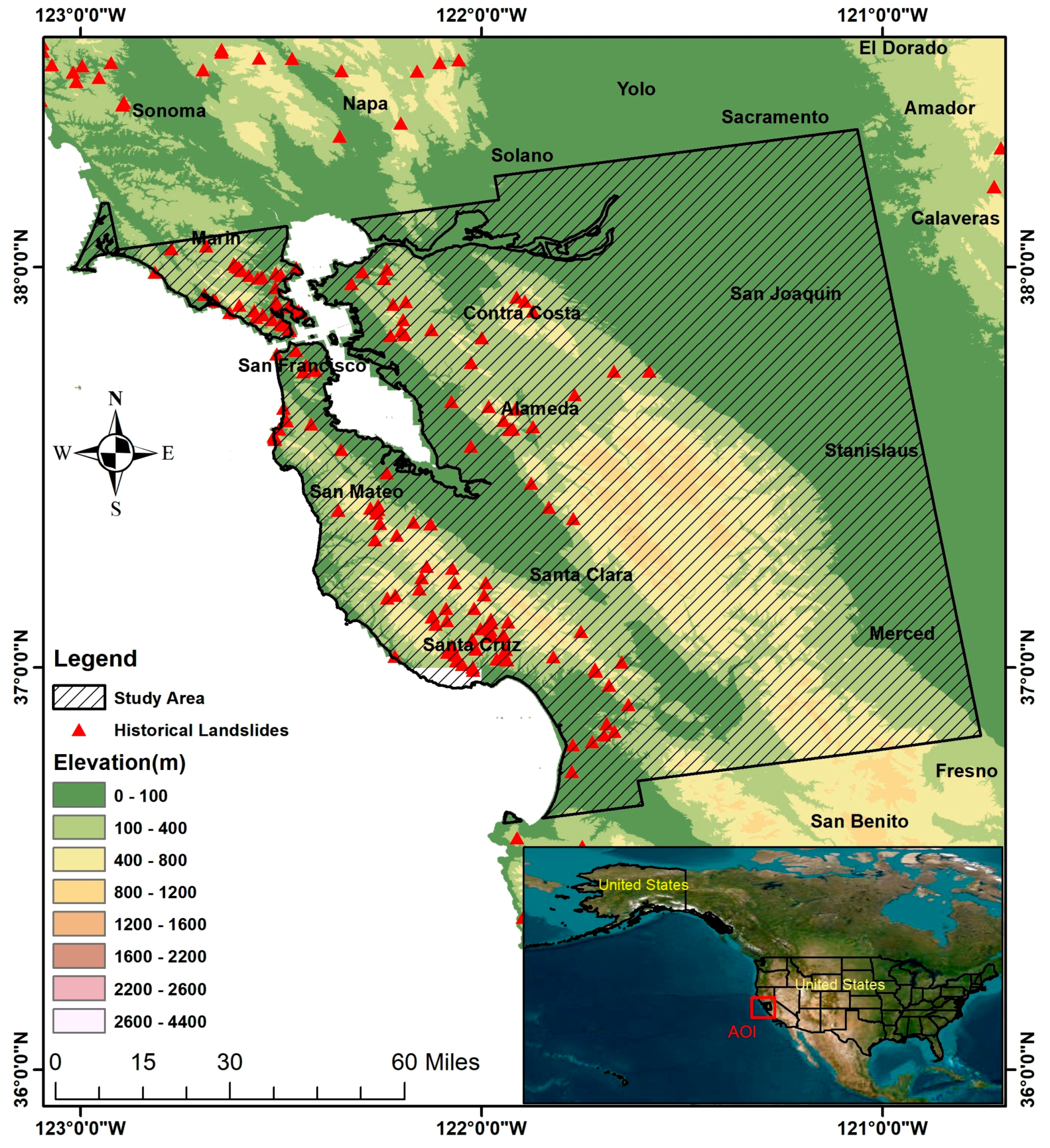
2. Study Area
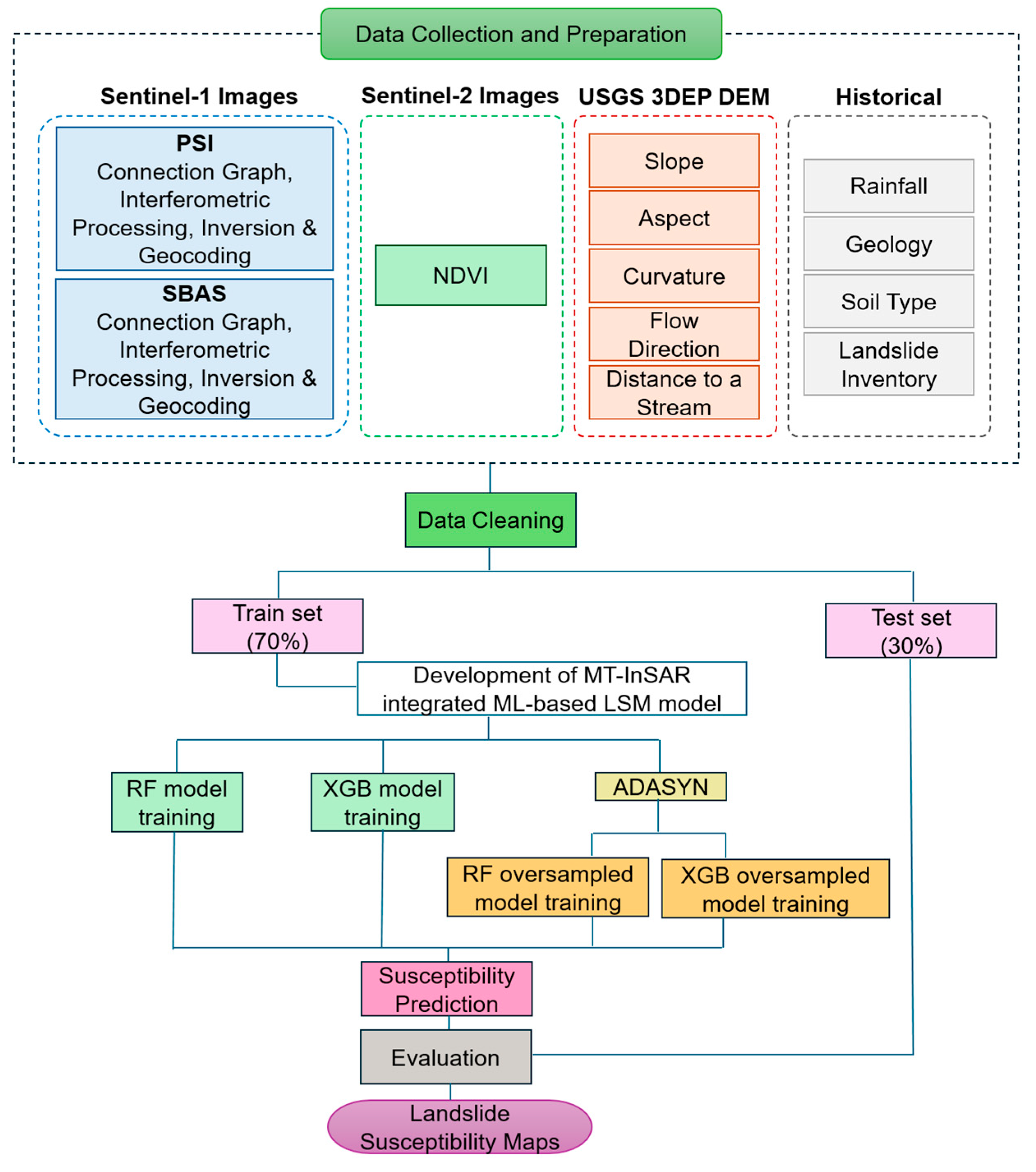
3. Data Collection and Preparation
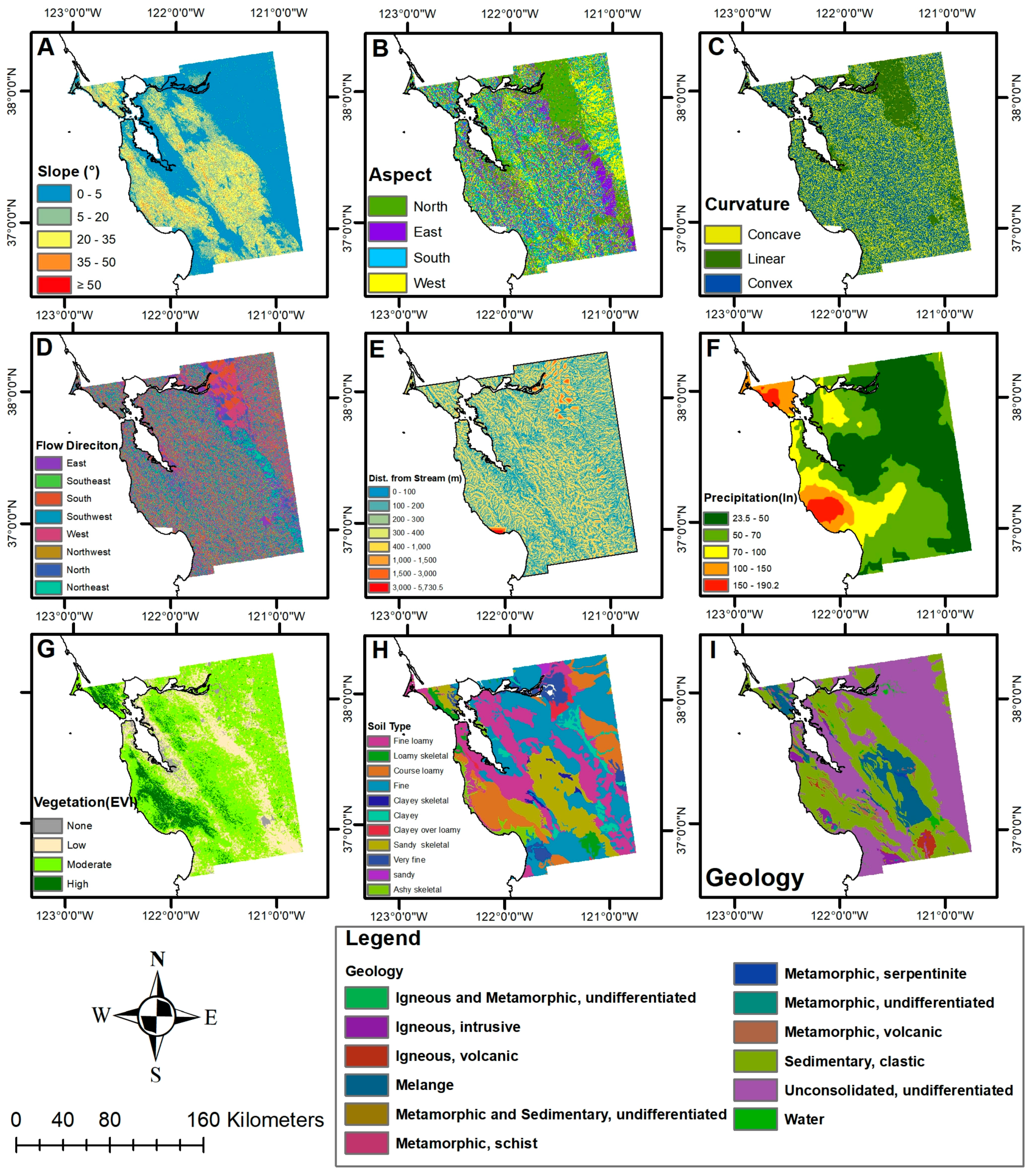
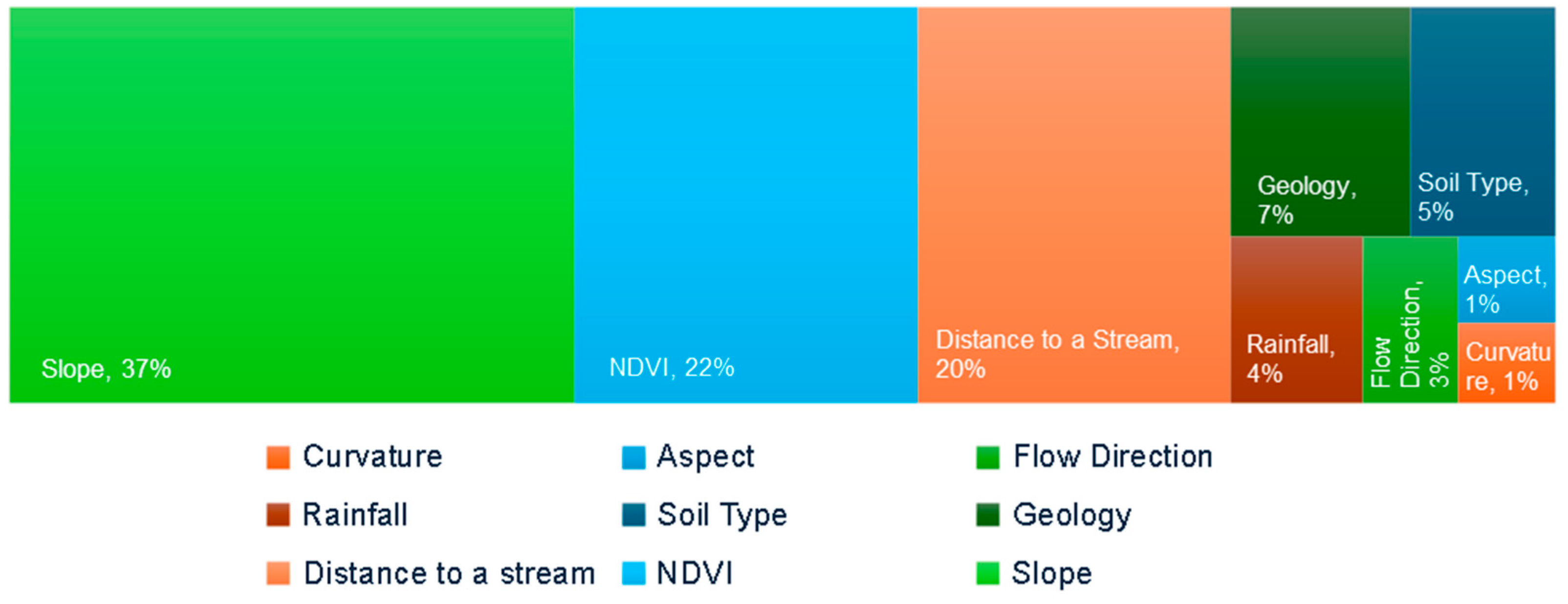
3.1. GIS Layers
3.1.1. Slope
3.1.2. Aspect
3.1.3. Curvature
3.1.4. Flow Direction
3.1.5. Distance to a Stream
3.1.6. Rainfall
3.1.7. Vegetation
3.1.8. Soil Type
3.1.9. Geology
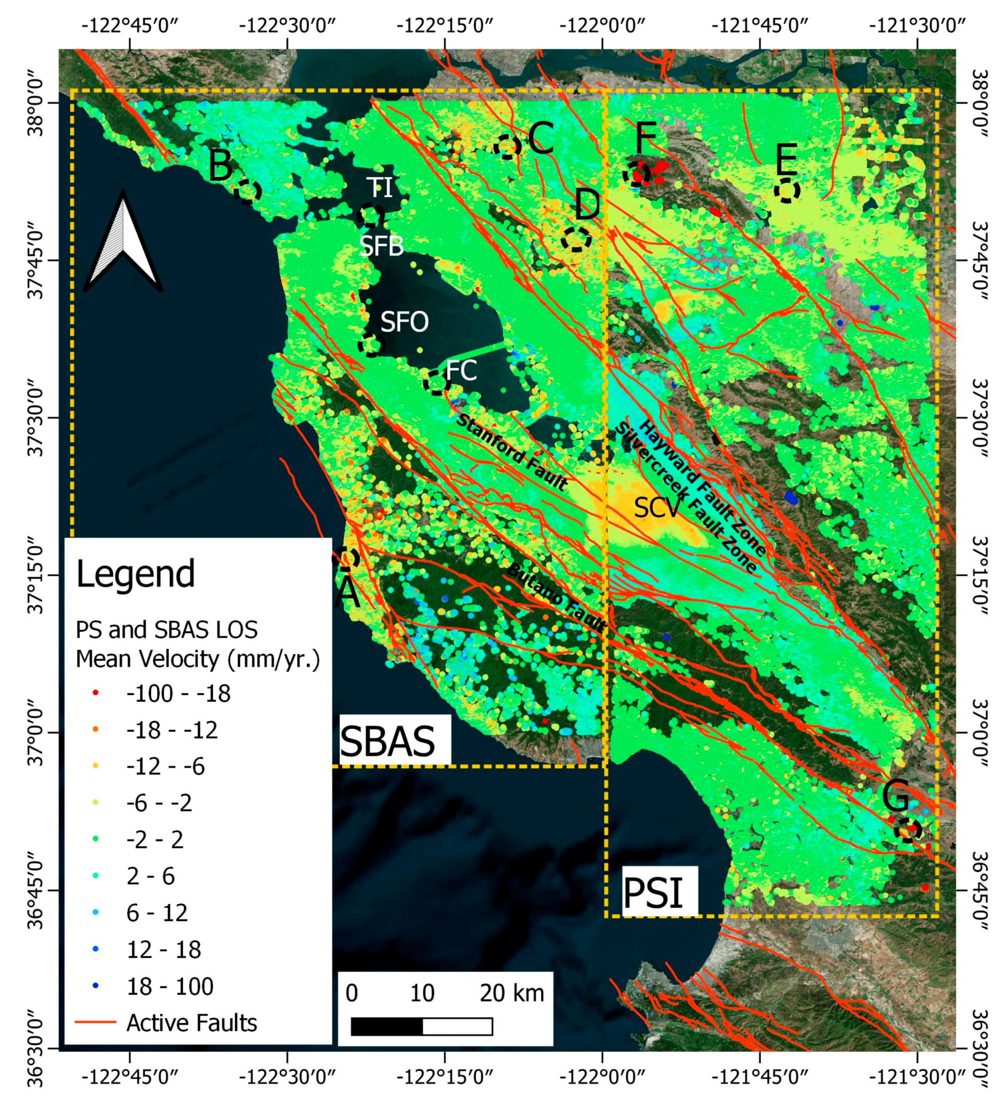
3.2. MT-InSAR Data
4. Methodology
4.1. MT-InSAR
4.2. Classification Criteria
4.3. Ensemble Learning Models
4.3.1. Random Forest (RF)
4.3.2. Extreme Gradient Boosting (XGB)
4.4. Model Parameter Tuning
4.5. Model Training
4.6. Model Validation
5. Results and Discussion
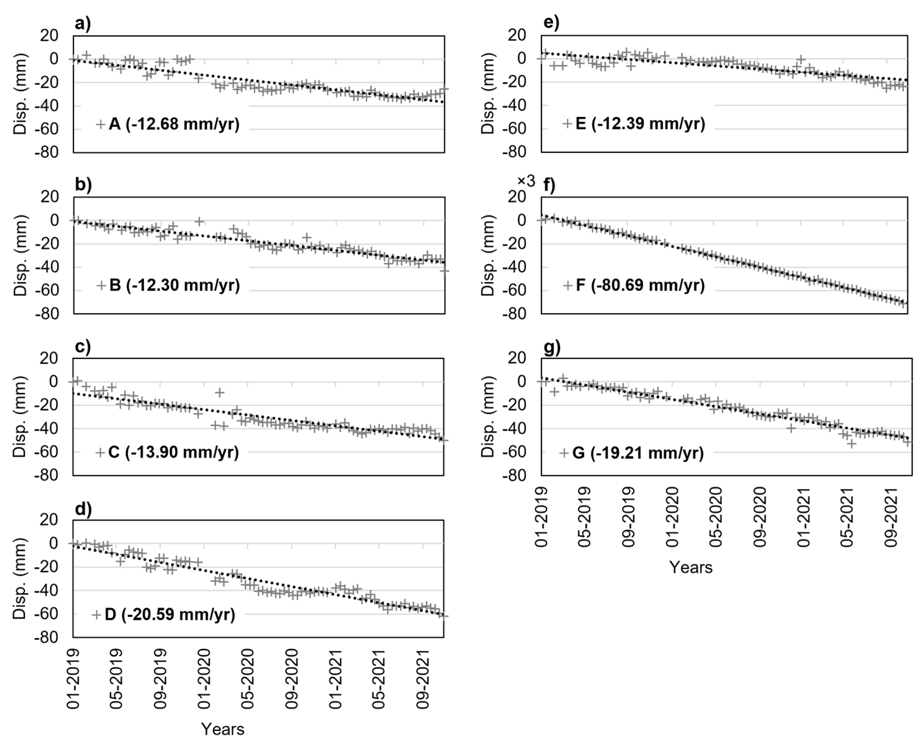
5.1. MT-InSAR Results
5.2. Model Accuracy Verification
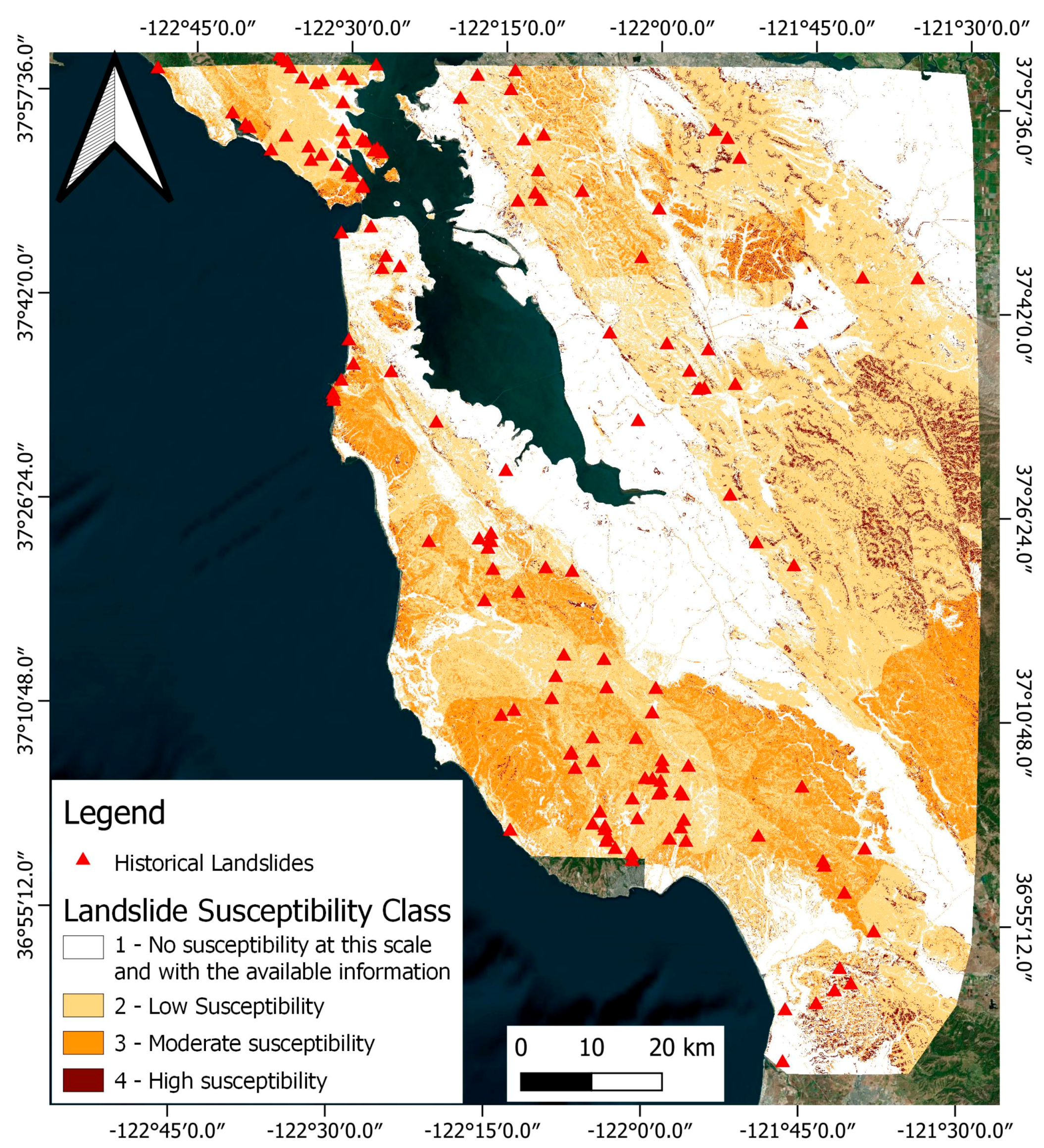
5.3. Landslide Susceptibility Mapping
6. Conclusions
Author Contributions
Funding
Data Availability Statement
Conflicts of Interest
References
- Hussain, S.; Pan, B.; Afzal, Z.; Ali, M.; Zhang, X.; Shi, X.; Ali, M. Landslide Detection and Inventory Updating Using the Time-Series InSAR Approach along the Karakoram Highway, Northern Pakistan. Sci. Rep. 2023, 13, 7485. [Google Scholar] [CrossRef] [PubMed]
- Popescu, M. Landslide Causal Factors and Landslide Remediation Options. In Proceedings of the 3rd International Conference on Landslides, Slope Stability and Safety of Infrastructures, Singapore, 11–12 July 2002; pp. 61–81. [Google Scholar]
- Chen, W.; Shahabi, H.; Shirzadi, A.; Hong, H.; Akgun, A.; Tian, Y.; Liu, J.; Zhu, A.-X.; Li, S. Novel Hybrid Artificial Intelligence Approach of Bivariate Statistical-Methods-Based Kernel Logistic Regression Classifier for Landslide Susceptibility Modeling. Bull. Eng. Geol. Environ. 2019, 78, 4397–4419. [Google Scholar] [CrossRef]
- Nhu, V.-H.; Mohammadi, A.; Shahabi, H.; Ahmad, B.B.; Al-Ansari, N.; Shirzadi, A.; Clague, J.J.; Jaafari, A.; Chen, W.; Nguyen, H. Landslide Susceptibility Mapping Using Machine Learning Algorithms and Remote Sensing Data in a Tropical Environment. Int. J. Environ. Res. Public Health 2020, 17, 4933. [Google Scholar] [CrossRef] [PubMed]
- Kouhartsiouk, D.; Perdikou, S. The Application of DInSAR and Bayesian Statistics for the Assessment of Landslide Susceptibility. Nat. Hazards 2021, 105, 2957–2985. [Google Scholar] [CrossRef]
- Brabb, E.E. The World Landslide Problem. Epis. J. Int. Geosci. 1991, 14, 52–61. [Google Scholar] [CrossRef]
- Ghorbani, Z.; Khosravi, A.; Maghsoudi, Y.; Mojtahedi, F.F.; Javadnia, E.; Nazari, A. Use of InSAR Data for Measuring Land Subsidence Induced by Groundwater Withdrawal and Climate Change in Ardabil Plain, Iran. Sci. Rep. 2022, 12, 13998. [Google Scholar] [CrossRef]
- Kirschbaum, D.B.; Adler, R.; Hong, Y.; Lerner-Lam, A. Evaluation of a Preliminary Satellite-Based Landslide Hazard Algorithm Using Global Landslide Inventories. Nat. Hazards Earth Syst. Sci. 2009, 9, 673–686. [Google Scholar] [CrossRef]
- Lee, S.; Min, K. Statistical Analysis of Landslide Susceptibility at Yongin, Korea. Environ. Geol. 2001, 40, 1095–1113. [Google Scholar] [CrossRef]
- Dai, F.C.; Lee, C.F. Landslide Characteristics and Slope Instability Modeling Using GIS, Lantau Island, Hong Kong. Geomorphology 2002, 42, 213–228. [Google Scholar] [CrossRef]
- Coe, J.; Michael, J.; Crovelli, R.; Savage, W.; Laprade, W.; Nashem, W. Probabilistic Assessment of Precipitation-Triggered Landslides Using Historical Records of Landslide Occurrence, Seattle, Washington. Environ. Eng. Geosci. 2004, 10, 103–122. [Google Scholar] [CrossRef]
- Ruff, M.; Czurda, K. Landslide Susceptibility Analysis with a Heuristic Approach in the Eastern Alps (Vorarlberg, Austria). Geomorphology 2008, 94, 314–324. [Google Scholar] [CrossRef]
- Evans, H.; Pennington, C.; Jordan, C.; Foster, C. Mapping a Nation’s Landslides: A Novel Multi-Stage Methodology. In Landslide Science and Practice: Volume 1: Landslide Inventory and Susceptibility and Hazard Zoning; Margottini, C., Canuti, P., Sassa, K., Eds.; Springer: Berlin/Heidelberg, Germany, 2013; pp. 21–27. ISBN 978-3-642-31325-7. [Google Scholar]
- Devaraj, S.; Yarrakula, K.; Martha, T.R.; Murugesan, G.P.; Vaka, D.S.; Surampudi, S.; Wadhwa, A.; Loganathan, P.; Budamala, V. Time Series SAR Interferometry Approach for Landslide Identification in Mountainous Areas of Western Ghats, India. J. Earth Syst. Sci. 2022, 131, 133. [Google Scholar] [CrossRef]
- Famiglietti, N.A.; Miele, P.; Defilippi, M.; Cantone, A.; Riccardi, P.; Tessari, G.; Vicari, A. Landslide Mapping in Calitri (Southern Italy) Using New Multi-Temporal InSAR Algorithms Based on Permanent and Distributed Scatterers. Remote Sens. 2024, 16, 1610. [Google Scholar] [CrossRef]
- Kim, J.-W.; Lu, Z.; Kaufmann, J. Evolution of Sinkholes over Wink, Texas, Observed by High-Resolution Optical and SAR Imagery. Remote Sens. Environ. 2019, 222, 119–132. [Google Scholar] [CrossRef]
- Vaka, D.S.; Rao, Y.S.; Bhattacharya, A. Surface Displacements of the 12 November 2017 Iran–Iraq Earthquake Derived Using SAR Interferometry. Geocarto Int. 2021, 36, 660–675. [Google Scholar] [CrossRef]
- Vaka, D.S.; Rao, Y.S.; Bhattacharya, A. Time Series Analysis of the Pre-Seismic and Post-Seismic Surface Deformation of the 2017 Iran–Iraq Earthquake Derived from Sentinel-1 InSAR Data. J. Earth Syst. Sci. 2023, 132, 64. [Google Scholar] [CrossRef]
- Ferretti, A.; Prati, C.; Rocca, F. Permanent Scatterers in SAR Interferometry. IEEE Trans. Geosci. Remote Sens. 2001, 39, 8–20. [Google Scholar] [CrossRef]
- Berardino, P.; Fornaro, G.; Lanari, R.; Sansosti, E. A New Algorithm for Surface Deformation Monitoring Based on Small Baseline Differential SAR Interferograms. IEEE Trans. Geosci. Remote Sens. 2002, 40, 2375–2383. [Google Scholar] [CrossRef]
- Lanari, R.; Casu, F.; Manzo, M.; Zeni, G.; Berardino, P.; Manunta, M.; Pepe, A. An Overview of the Small BAseline Subset Algorithm: A DInSAR Technique for Surface Deformation Analysis. Pure Appl. Geophys. 2007, 164, 637–661. [Google Scholar] [CrossRef]
- Bouali, E.H.; Oommen, T.; Escobar-Wolf, R. Mapping of Slow Landslides on the Palos Verdes Peninsula Using the California Landslide Inventory and Persistent Scatterer Interferometry. Landslides 2018, 15, 439–452. [Google Scholar] [CrossRef]
- Moretto, S.; Bozzano, F.; Mazzanti, P. The Role of Satellite InSAR for Landslide Forecasting: Limitations and Openings. Remote Sens. 2021, 13, 3735. [Google Scholar] [CrossRef]
- Zhang, L.; Dai, K.; Deng, J.; Ge, D.; Liang, R.; Li, W.; Xu, Q. Identifying Potential Landslides by Stacking-InSAR in Southwestern China and Its Performance Comparison with SBAS-InSAR. Remote Sens. 2021, 13, 3662. [Google Scholar] [CrossRef]
- Hussain, M.A.; Chen, Z.; Zheng, Y.; Shoaib, M.; Shah, S.U.; Ali, N.; Afzal, Z. Landslide Susceptibility Mapping Using Machine Learning Algorithm Validated by Persistent Scatterer In-SAR Technique. Sensors 2022, 22, 3119. [Google Scholar] [CrossRef] [PubMed]
- Yao, J.; Yao, X.; Liu, X. Landslide Detection and Mapping Based on SBAS-InSAR and PS-InSAR: A Case Study in Gongjue County, Tibet, China. Remote Sens. 2022, 14, 4728. [Google Scholar] [CrossRef]
- Miao, F.; Ruan, Q.; Wu, Y.; Qian, Z.; Kong, Z.; Qin, Z. Landslide Dynamic Susceptibility Mapping Base on Machine Learning and the PS-InSAR Coupling Model. Remote Sens. 2023, 15, 5427. [Google Scholar] [CrossRef]
- Wu, X.; Qi, X.; Peng, B.; Wang, J. Optimized Landslide Susceptibility Mapping and Modelling Using the SBAS-InSAR Coupling Model. Remote Sens. 2024, 16, 2873. [Google Scholar] [CrossRef]
- Sarkar, S.; Kanungo, D.P. An Integrated Approach for Landslide Susceptibility Mapping Using Remote Sensing and GIS. Photogramm. Eng. Remote Sens. 2004, 70, 617–625. [Google Scholar] [CrossRef]
- Tyoda, Z. Landslide Susceptibility Mapping: Remote Sensing and GIS Approach. Ph.D. Thesis, Stellenbosch University, Stellenbosch, South Africa, 2013. [Google Scholar]
- Nhu, V.-H.; Shirzadi, A.; Shahabi, H.; Singh, S.K.; Al-Ansari, N.; Clague, J.J.; Jaafari, A.; Chen, W.; Miraki, S.; Dou, J. Shallow Landslide Susceptibility Mapping: A Comparison between Logistic Model Tree, Logistic Regression, Naïve Bayes Tree, Artificial Neural Network, and Support Vector Machine Algorithms. Int. J. Environ. Res. Public Health 2020, 17, 2749. [Google Scholar] [CrossRef]
- Ali, N.; Chen, J.; Fu, X.; Ali, R.; Hussain, M.A.; Daud, H.; Hussain, J.; Altalbe, A. Integrating Machine Learning Ensembles for Landslide Susceptibility Mapping in Northern Pakistan. Remote Sens. 2024, 16, 988. [Google Scholar] [CrossRef]
- Whiteley, J.S.; Watlet, A.; Kendall, J.M.; Chambers, J.E. Brief Communication: The Role of Geophysical Imaging in Local Landslide Early Warning Systems. Nat. Hazards Earth Syst. Sci. 2021, 21, 3863–3871. [Google Scholar] [CrossRef]
- Handwerger, A.L.; Huang, M.-H.; Fielding, E.J.; Booth, A.M.; Bürgmann, R. A Shift from Drought to Extreme Rainfall Drives a Stable Landslide to Catastrophic Failure. Sci. Rep. 2019, 9, 1569. [Google Scholar] [CrossRef] [PubMed]
- Kang, Y.; Lu, Z.; Zhao, C.; Xu, Y.; Kim, J.; Gallegos, A.J. InSAR Monitoring of Creeping Landslides in Mountainous Regions: A Case Study in Eldorado National Forest, California. Remote Sens. Environ. 2021, 258, 112400. [Google Scholar] [CrossRef]
- Cohen-Waeber, J.; Sitar, N.; Bürgmann, R. GPS Instrumentation and Remote Sensing Study of Slow Moving Landslides in the Eastern San Francisco Bay Hills, California, USA. In Proceedings of the 18th International Conference on Soil Mechanics and Geotechnical Engineering, Paris, France, 2–6 September 2013; pp. 2169–2172. [Google Scholar]
- Cohen-Waeber, J.; Bürgmann, R.; Sitar, N.; Ferretti, A.; Giannico, C.; Bianchi, M. 18 Geodetic Tracking and Characterization of Precipitation Triggered Slow Moving Landslide Displacements in the Eastern San Francisco Bay Hills, California, USA; Berkeley Seismological Laboratory: Berkeley, CA, USA, 2013; Volume 42. [Google Scholar]
- Hilley, G.E.; Bürgmann, R.; Ferretti, A.; Novali, F.; Rocca, F. Dynamics of Slow-Moving Landslides from Permanent Scatterer Analysis. Science 2004, 304, 1952–1955. [Google Scholar] [CrossRef] [PubMed]
- Quigley, K.C.; Bürgmann, R.; Giannico, C.; Novali, F.; Knudsen, I.K. Seasonal Acceleration and Structure of Slow Moving Landslides in the Berkeley Hills. In California Geological Survey Special Report, Proceedings of the Third Conference on Earthquake Hazards, Eastern San Francisco Bay Area, CA, USA, 22–24 October 2008; California Department of Conservation: Sacramento, CA, USA, 2010; Volume 219. [Google Scholar]
- Giannico, C.; Ferretti, A. SqueeSAR Analysis Area: Berkeley; Tele-Rilevamento Europa: Milano, Italy, 2011. [Google Scholar]
- Cohen-Waeber, J.; Bürgmann, R.; Chaussard, E.; Giannico, C.; Ferretti, A. Spatiotemporal Patterns of Precipitation-Modulated Landslide Deformation from Independent Component Analysis of InSAR Time Series. Geophys. Res. Lett. 2018, 45, 1878–1887. [Google Scholar] [CrossRef]
- Bürgmann, R.; Hilley, G.; Ferretti, A.; Novali, F. Resolving Vertical Tectonics in the San Francisco Bay Area from Permanent Scatterer InSAR and GPS Analysis. Geology 2006, 34, 221–224. [Google Scholar] [CrossRef]
- Horton, J.D.; San Juan, C.A.; Stoeser, D.B. The State Geologic Map Compilation (SGMC) Geodatabase of the Vonterminous United States (Version 1.1, August 2017); U.S. Geological Survey Data Series; U.S. Geological Survey: Washington, DC, USA, 2017; Volume 1052, 46p. [CrossRef]
- Huang, G.; Zheng, M.; Peng, J. Effect of Vegetation Roots on the Threshold of Slope Instability Induced by Rainfall and Runoff. Geofluids 2021, 2021, 6682113. [Google Scholar] [CrossRef]
- Liu, Y.; Deng, Z.; Wang, X. The Effects of Rainfall, Soil Type and Slope on the Processes and Mechanisms of Rainfall-Induced Shallow Landslides. Appl. Sci. 2021, 11, 11652. [Google Scholar] [CrossRef]
- Segoni, S.; Pappafico, G.; Luti, T.; Catani, F. Landslide Susceptibility Assessment in Complex Geological Settings: Sensitivity to Geological Information and Insights on Its Parameterization. Landslides 2020, 17, 2443–2453. [Google Scholar] [CrossRef]
- Yao, Z.; Chen, M.; Zhan, J.; Zhuang, J.; Sun, Y.; Yu, Q.; Yu, Z. Refined Landslide Susceptibility Mapping by Integrating the SHAP-CatBoost Model and InSAR Observations: A Case Study of Lishui, Southern China. Appl. Sci. 2023, 13, 12817. [Google Scholar] [CrossRef]
- Veselskỳ, M.; Bandura, P.; Burian, L.; Harciníková, T.; Bella, P. Semi-Automated Recognition of Planation Surfacesand Other Flat Landforms: A Case Study from theAggtelek Karst, Hungary. Open Geosci. 2015, 7, 63. [Google Scholar] [CrossRef]
- Huang, F.; Xie, G.; Xiao, R. Research on Ensemble Learning. In Proceedings of the 2009 International Conference on Artificial Intelligence and Computational Intelligence, Shanghai, China, 7–8 November 2009; Volume 3, pp. 249–252. [Google Scholar]
- Belgiu, M.; Drăguţ, L. Random Forest in Remote Sensing: A Review of Applications and Future Directions. ISPRS J. Photogramm. Remote Sens. 2016, 114, 24–31. [Google Scholar] [CrossRef]
- Nam, K.; Kim, J.; Chae, B.-G. Exploring Class Imbalance with Under-Sampling, over-Sampling, and Hybrid Sampling Based on Mahalanobis Distance for Landslide Susceptibility Assessment: A Case Study of the 2018 Iburi Earthquake Induced Landslides in Hokkaido, Japan. Geosci. J. 2024, 28, 71–94. [Google Scholar] [CrossRef]
- Zhang, Y.; Liang, S.; Zhu, Z.; Ma, H.; He, T. Soil Moisture Content Retrieval from Landsat 8 Data Using Ensemble Learning. ISPRS J. Photogramm. Remote Sens. 2022, 185, 32–47. [Google Scholar] [CrossRef]
- Zhang, W.; He, Y.; Wang, L.; Liu, S.; Meng, X. Landslide Susceptibility Mapping Using Random Forest and Extreme Gradient Boosting: A Case Study of Fengjie, Chongqing. Geol. J. 2023, 58, 2372–2387. [Google Scholar] [CrossRef]
- Dhieb, N.; Ghazzai, H.; Besbes, H.; Massoud, Y. Extreme Gradient Boosting Machine Learning Algorithm for Safe Auto Insurance Operations. In Proceedings of the 2019 IEEE International Conference on Vehicular Electronics and Safety (ICVES), Cairo, Egypt, 4–6 September 2019; pp. 1–5. [Google Scholar]
- Ahmad, M.; Al-Mansob, R.A.; Kashyzadeh, K.R.; Keawsawasvong, S.; Sabri Sabri, M.M.; Jamil, I.; Alguno, A.C. Extreme Gradient Boosting Algorithm for Predicting Shear Strengths of Rockfill Materials. Complexity 2022, 2022, 9415863. [Google Scholar] [CrossRef]
- Sharma, N.; Saharia, M.; Ramana, G.V. High Resolution Landslide Susceptibility Mapping Using Ensemble Machine Learning and Geospatial Big Data. Catena 2024, 235, 107653. [Google Scholar] [CrossRef]
- Shirzaei, M.; Bürgmann, R.; Fielding, E.J. Applicability of Sentinel-1 Terrain Observation by Progressive Scans Multitemporal Interferometry for Monitoring Slow Ground Motions in the San Francisco Bay Area. Geophys. Res. Lett. 2017, 44, 2733–2742. [Google Scholar] [CrossRef]
- Shirzaei, M.; Bürgmann, R. Global Climate Change and Local Land Subsidence Exacerbate Inundation Risk to the San Francisco Bay Area. Sci. Adv. 2018, 4, eaap9234. [Google Scholar] [CrossRef]
- Li, Q.; Huang, D.; Pei, S.; Qiao, J.; Wang, M. Using Physical Model Experiments for Hazards Assessment of Rainfall-Induced Debris Landslides. J. Earth Sci. 2021, 32, 1113–1128. [Google Scholar] [CrossRef]
- Wu, L.Z.; Xu, Q.; Zhu, J.D. Incorporating Hydro-Mechanical Coupling in an Analysis of the Effects of Rainfall Patterns on Unsaturated Soil Slope Stability. Arab. J. Geosci. 2017, 10, 386. [Google Scholar] [CrossRef]


| Class | Criteria | Susceptibility |
|---|---|---|
| 1 | Absolute velocity interval: from 0 to 2 mm/year AND Slope interval: (0, 5]° | No susceptibility at this scale, and with the available information |
| 2 | Absolute velocity interval: from 2 to 5 mm/year AND Slope interval: (5, 90]° | Low susceptibility |
| 3 | Absolute velocity interval: (5, 15] mm/year AND Slope interval: (5, 90]° | Moderate susceptibility |
| 4 | Absolute velocity interval:(>15) mm/year AND Slope interval: (5, 90]° OR Historical landslide event AND Slope interval: (5, 90]° | High susceptibility |
| Study | Velocity Classification | Susceptibility |
|---|---|---|
| This study | 0–2 mm/y | No susceptibility at this scale, and with the available information |
| 2–5 mm/y | Low susceptibility | |
| 5–15 mm/y | Moderate susceptibility | |
| >15 mm/y | High susceptibility | |
| Yao et al. [47] | <2.46 mm/y | Very low susceptibility |
| 5.39 mm/y to 2.46 mm/y | Low susceptibility | |
| 9.14 mm/y to 5.39 mm/y | Moderate susceptibility | |
| 14.88 mm/y to 9.14 mm/y | High susceptibility | |
| >14.88 mm/yr | Very high susceptibility | |
| Moretto et al. [23] | <3 mm/y | Stable |
| 3–5 mm/y | Moderate deformation | |
| >5 mm/y | High deformation |
Disclaimer/Publisher’s Note: The statements, opinions and data contained in all publications are solely those of the individual author(s) and contributor(s) and not of MDPI and/or the editor(s). MDPI and/or the editor(s) disclaim responsibility for any injury to people or property resulting from any ideas, methods, instructions or products referred to in the content. |
© 2024 by the authors. Licensee MDPI, Basel, Switzerland. This article is an open access article distributed under the terms and conditions of the Creative Commons Attribution (CC BY) license (https://creativecommons.org/licenses/by/4.0/).
Share and Cite
Vaka, D.S.; Yaragunda, V.R.; Perdikou, S.; Papanicolaou, A. InSAR Integrated Machine Learning Approach for Landslide Susceptibility Mapping in California. Remote Sens. 2024, 16, 3574. https://doi.org/10.3390/rs16193574
Vaka DS, Yaragunda VR, Perdikou S, Papanicolaou A. InSAR Integrated Machine Learning Approach for Landslide Susceptibility Mapping in California. Remote Sensing. 2024; 16(19):3574. https://doi.org/10.3390/rs16193574
Chicago/Turabian StyleVaka, Divya Sekhar, Vishnuvardhan Reddy Yaragunda, Skevi Perdikou, and Alexandra Papanicolaou. 2024. "InSAR Integrated Machine Learning Approach for Landslide Susceptibility Mapping in California" Remote Sensing 16, no. 19: 3574. https://doi.org/10.3390/rs16193574