Detection of Wet Snow by Weakly Supervised Deep Learning Change Detection Algorithm with Sentinel-1 Data

Abstract

The snowmelt process plays a crucial role in hydrological forecasting, climate change, disaster management, and other related fields. Accurate detection of wet snow distribution and its changes is essential for understanding and modeling the snow melting process. To address the limitations of conventional fixed-threshold methods, which suffer from poor adaptability and significant interference from scattering noise, we propose a weakly supervised deep learning change detection algorithm with Sentinel-1 multi-temporal data. This algorithm incorporates the Multi-Region Convolution Module (MRC) to enhance the central region while effectively suppressing edge noise. Furthermore, it integrates the ResNet residual network to capture deeper image features, facilitating wet snow identification through feature fusion. Various combinations of differential images, polarization data, elevation, and slope information during and after snowmelt were input into the model and tested. The results suggest that the combination of differential images, VV polarization data, and slope information has greater advantages in wet snow extraction. Comparisons between our method, the fixed-threshold method, OTSU algorithm, and FCM algorithm against the results of Landsat images indicates that the overall accuracy of our method improves significantly when the proportion of wet snow cover is large, and the average overall accuracy of wet snow extraction is 85.2%. This study provides clues for the accurate identification of wet snow during the mid-snowmelt phase.

1. Introduction

Snow cover is a crucial component of the cryosphere and significantly influences climate [1,2]. It serves as a vital freshwater resource during spring in arid and semi-arid regions [3,4]. Dynamic changes in snow cover serve as indicators for estimating and forecasting snowmelt runoff volumes [5], essential for water resource management and climate change research [6]. Rapid snowmelt can cause floods or avalanches; thus, accurate monitoring of wet snow during snow melting is crucial for hydrological process assessments, wet snow avalanche forecasts, and natural disaster management.

Snow cover monitoring primarily relies on station observations and remote sensing retrieval. Although traditional field measurements are highly accurate, they still present challenges for large-scale monitoring [7]. With the increase in launch satellites and the availability of data, extensive research has been conducted on snow cover extraction with optical and microwave remote sensing data [8,9]. Numerous snow cover products have been developed with optical data [10,11]. However, spectral similarities between snow and clouds, such as ice and cirrus clouds, lead to misclassification. Optical images cannot identify ground objects under clouds and distinguish between dry and wet snow [12,13]. In contrast, microwave remote sensing, unaffected by atmospheric conditions and weather, enables constant, all-weather imaging. Passive microwave sensors have low spatial resolution, limiting their application to basin-scale research [14]. In contrast, active microwave sensors like Synthetic Aperture Radar (SAR) offer higher spatial resolution and are sensitive to liquid water in snow. This makes SAR effective for detecting wet snow, as its dielectric properties change significantly during melting [6].

As temperatures rise, the surface of the snowpack begins to melt, gradually transitioning into wet snow [15]. Snow is defined as wet when its volumetric water content exceeds 1% or its temperature rises above 0 °C [16]. During snow melting, the increased liquid water content causes greater dielectric losses, reducing backscatter signals, which makes wet snow more detectable in microwave remote sensing [17]. Numerous studies have explored wet snow detection with SAR data [18,19]. Common methods often employ fixed-threshold-based change detection algorithms. Nagler et al. [6] identified wet snow by calculating the ratio from Radarsat images during snow-covered and snow-free periods, with an empirical threshold of −3 dB. In the Tuxbach and Schlegeis regions of the Austrian Alps, accuracy reached 85.4% and 81.4%, respectively. However, their method required additional empirical rules to mitigate misclassification in farmlands and high-altitude areas, and did not explore the applicability across different snowmelt phases. Enhancements by Nagler et al. [18] included integrating local incidence angle information with VV and VH polarizations, applying a −2 dB threshold, suggesting that multi-polarization SAR images could improve wet snow detection accuracy. Torralbo et al. [20] explored thresholds for different snowmelt periods in the Sierra Nevada, finding that optimal thresholds ranged from −2 dB to −3.88 dB, indicating that fixed thresholds do not universally apply across various snowmelt phases. Liu et al. [21] used the OTSU algorithm for adaptive wet snow extraction across different landcover types, achieving an overall accuracy of 73.9% after incorporating terrain information, but this was only tested on a single snowmelt phase. With advancements in machine learning, Gallet et al. [22] utilized information from the Crocus physical snow model to label Sentinel-1 data, employing seven common machine learning models, such as Adaboost and K-nearest neighbors (KNN) for supervised training. The overall accuracy of wet snow detection using KNN was 73.2%, while the labeled data exhibited some uncertainties.

In summary, existing methods for wet snow detection primarily face several limitations: (1) Research predominantly focuses on specific regions like the Alps and the Himalayas [16], with most studies restricted to analyses of a single scene, lacking comparative evaluations across different snowmelt phases. (2) Traditional fixed-threshold methods rely on experiential rules, and inaccurate threshold settings can lead to substantial misestimations of wet snow coverage. These thresholds lack universality across various regions and snowmelt periods. (3) Current methods generally identify wet snow of individual pixels without considering the spatial relationships between pixels, influenced by speckle noise. This often results in incomplete and fragmented extraction results.

Recently, deep learning change detection algorithms have been extensively researched in microwave remote sensing data identification [23,24]. Convolutional Neural Networks (CNNs) have the ability to hierarchically extract and efficiently utilize spatial neighborhood information, providing a significant advantage in processing complex datasets [25]. Many researchers have employed and improved models like U-Net and DeepLabV3+ for snow cover detection, achieving higher accuracy [26,27]. Given the challenges in acquiring large volumes of high-quality labeled datasets, weakly supervised deep learning has emerged as an effective approach [28]. This method reduces the reliance on extensive, high-quality labeled data, significantly lowering the costs of data labeling. It is especially advantageous for remote sensing applications, where labeling data can be challenging and expensive.

This study utilizes C-band SAR data from Sentinel-1, constructing differential images by combining local incidence angle data with VV and VH polarization. We propose a novel method for wet snow detection using a weakly supervised, dual-branch deep learning model that considers backscatter and topographic information. This method was applied to identify wet snow across multiple scenes at different snow melting phases, validated with the results of Landsat image. Additionally, the results were compared with the wet snow identification results obtained by traditional threshold methods, OTSU, and Fuzzy C-means (FCM) algorithms. The objectives of this study include: (1) To develop a weakly supervised dual-branch deep learning model for wet snow detection across different snowmelt periods. (2) To analyze the advantages and limitations of the wet snow detection model.

2. Study Area and Data Sources

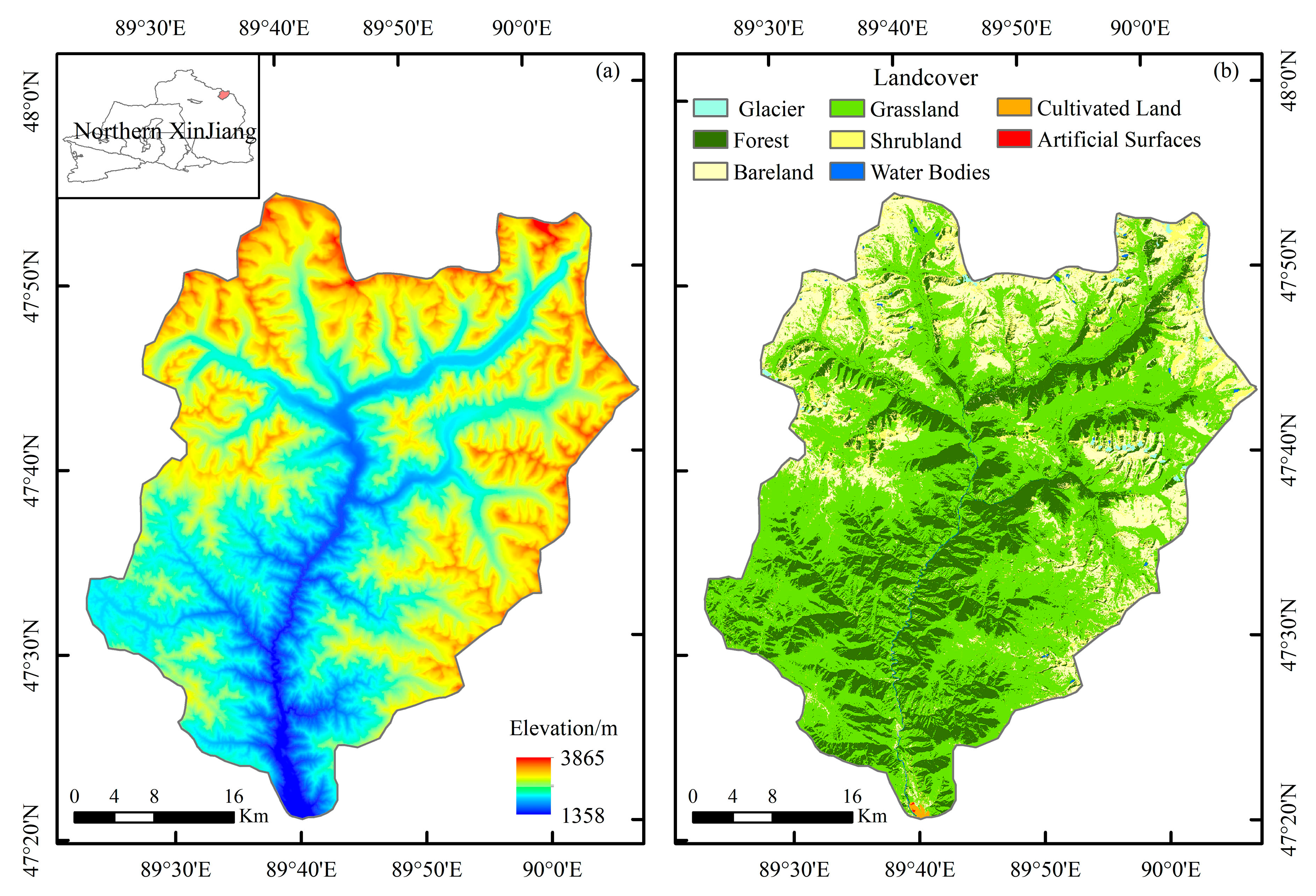
2.1. Study Area

The study area is located upstream of the confluence of the Kayertes River and Irtysh River, on the southern slope of the Altai Mountains. Elevations within the area range from 1358 to 3865 m, with higher elevations in the north and lower in the south. It is one of the two main source rivers of the Irtysh River. Figure 1 shows the geographical location, topography, and land-cover types within the basin. Approximately half of the land is covered by low grasslands, with south-facing slopes primarily consisting of grasslands and shrubs, while north-facing slopes are dominated by forests, predominantly Siberian larch and Siberian spruce [29]. The regional climate is influenced by the westerlies, leading to cold winter conditions with temperatures dropping to as low as −50 °C [30]. The area receives an average annual precipitation of about 360 mm, unevenly distributed throughout the year. During winter, the entire basin is covered by a thick, stable snow layer starting in November [31,32]. In lower elevations, the snow cover persists from November to March, while, at higher altitudes, it remains until July.

2.2. Data Sources

2.2.1. Sentinel-1 Data

The Sentinel-1 satellite consists of the polar-orbiting satellites Sentinel-1A and Sentinel-1B, each equipped with a C-band SAR capable of operating in four imaging modes: Strip Map (SM), Interferometric Wide (IW), Extra Wide (EW), and Wave (WV). The revisit period of each satellite is 12d. We utilize Level-1 Ground Range Detected (GRD) data products acquired in the IW mode with VV and VH polarizations. Compared to single look complex (SLC) data, GRD data do not contain phase information but have a smaller data volume. The study area is fully covered by Sentinel-1 relative orbits D121 (Sentinel-1B descending), D19 (Sentinel-1B descending), and A143 (Sentinel-1A ascending). To compare with Landsat imagery results, we selected Sentinel-1 data from snowmelt phases on 15 May 2018, 2 July 2018, 3 June 2019, 20 June 2019, 22 April 2020, 9 May 2021, and 4 June 2021 for wet snow identification and validation.

Sentinel-1 data were preprocessed using SNAP software version 9.0.0, including precise orbit correction, thermal noise removal, radiometric calibration, terrain correction, and conversion of backscatter coefficients to decibels, resulting in 10 m resolution backscatter coefficient images. Precise Orbit Determination (POD) data, accurate to within 5 cm, correct orbital information to mitigate systematic errors. To mitigate errors caused by terrain effects, such as shadows and layover in Sentinel-1 imagery, radiometric terrain correction and filtering were applied. Specifically, SRTM DEM data were utilized for radiometric terrain correction, correcting geometric distortions induced by complex topography. Furthermore, the Refined Lee filtering algorithm was employed to smooth the imagery and reduce artifacts and noise in shadowed and layover regions. The co-registration of Sentinel-1 ascending and descending orbit data minimizes geographic discrepancies caused by orbital differences. This process involves aligning satellite images from different orbits and viewing angles to a common reference coordinate system, ensuring spatial consistency across the images. These preprocessing steps effectively reduce errors resulting from terrain variations and data inconsistencies. Since the radar signal emitted by the Sentinel-1 satellite travels long distances, the processed data represent the backscatter coefficient in linear scale units, typically small positive values. For better visualization and analysis, these data are converted to decibels (dB), resulting in a backscatter coefficient range that approximates a Gaussian distribution.

2.2.2. Landsat 8 OLI Data

The analysis of Landsat images shows that snowmelt in the basin begins in March at lower elevations and continues until it is completely melted by August. Accordingly, March to July was designated as the snow melting period, with August identified as the snow-free period. For validation of wet snow extraction accuracy, Landsat 8 OLI images from 15 May 2018, 2 July 2018, 3 June 2019, 19 June 2019, 18 April 2020, 7 May 2021, and 8 June 2021 were selected. Snow extraction utilized the SNOMAP algorithm [33], which requires NDSI values of at least 0.4 and NIR band reflectance of at least 0.11 to reduce the misidentification of water bodies. Additionally, snow coverage in the study area was further corrected through visual interpretation to enhance the accuracy of the evaluation.

2.2.3. Other Auxiliary Data

Additional auxiliary data for this study include the SRTM DEM and land-cover datasets. The 30 m resolution SRTM DEM data are employed for terrain correction in the preprocessing of Sentinel-1 data and for extracting topographical features such as elevation and slope within the basin. The GlobalLand30 land-cover dataset has a resolution of 30 m and comprises 10 primary land-cover types. Within the study area, the dataset includes eight types: cultivated land, forest, grassland, shrubland, water bodies, artificial surfaces, bare land, and glaciers. The DEM data were sourced from the USGS Earth Explorer website (http://earthexplorer.usgs.gov/, accessed on 21 September 2024), and the land-cover dataset from the website (https://www.geodata.cn/, accessed on 21 September 2024). The specific information regarding the data utilized in this study is presented in

Table 1. Introduction of datasets and their specific parameter information.

	Data Type	Data Parameters		Acquisition Date
Radar Remote Sensing Image				15 May 2018
		Imaging Mode: IW		2 July 2018
		Center Frequency: C-band		3 June 2019
	Sentinel-1 GRD	Polarization Mode: VV + VH		20 June 2019
		Spatial Resolution: 5 × 20 m		22 April 2020
		Revisit Cycle: 12 days		9 May 2021
				4 June 2021
Optical Remote Sensing Image				15 May 2018
		Bands	Green Band Near Infrared Band Shortwave Infrared Band	2 July 2018
				3 June 2019
	Landsat 8 OLI			19 June 2019
		Spatial Resolution: 30 m		18 April 2020
		Revisit Cycle: 18 days		7 May 2021
				8 June 2021
Auxiliary Data	SRTM DEM	Spatial Resolution: 30 m		-
	Land-Cover Data	Spatial Resolution: 30 m		-

.

3. Methodology

3.1. Acquisition of Differential Image

During the snowmelt process, the increase in liquid water content significantly reduces the backscatter coefficients in wet snow areas, creating a distinct contrast with dry snow or snow-free regions [6,19]. This contrast enables the effective differentiation of wet snow from other surface features. Consequently, differential images constructed from Sentinel-1 polarization data were input for the wet snow detection studies. The differential images are generated by calculating the difference between the backscatter coefficient images during the snowmelt periods and the snow-free periods. To suppress speckle noise, the reference image is derived from the average backscatter coefficients of multiple snow-free period images [34]. Considering the compensatory effect of cross-polarization in complex terrains and the sensitivity of VH polarization to water content changes, differential images, denoted as Rc, are calculated by combining local incidence angles with VV and VH polarizations [18]. The specific formulas are provided in Formula (1).

$$\begin{array}{l}{R}_C=W{R}_{VH}+(1-W)R_{VV}\\ R_{VH}={\sigma }_{VH}^0(dB)-{\sigma }_{\mathrm{ref}VH}^0(dB) \\ R_{VV}={\sigma }_{VV}^0(dB)-{\sigma }_{\mathrm{ref}VV}^0(dB)\end{array}$$

(1)

R_c is the differential backscatter coefficient of the image during and after snowmelt. R_VH and R_VV are the VH and VV polarization differential backscatter coefficients, respectively. σ⁰ and σ⁰_ref are the backscatter coefficients during the snowmelt and snow-free periods, respectively. The weighting factor W is computed based on the local incidence angle. The value of W is calculated as follows:

$$\begin{array}{l}\mathrm{if}(\theta <{\theta }_1),W=1.0\\ \mathrm{if}({\theta }_1\le \theta <{\theta }_2),W=K[1+{\displaystyle \frac{({\theta }_2-\theta )}{{\theta }_2-{\theta }_1}}] \\ \mathrm{if}(\theta >{\theta }_2),W=K\end{array}$$

(2)

where ${\theta }_1$ is 20°; ${\theta }_2$ is 45°; and K is 0.5.

3.2. Weakly Supervised Dual-Branch Deep Learning Change Detection Algorithm

We proposed a new model that utilizes a weakly supervised deep learning change detection algorithm to extract wet snow extents from imagery. By performing an unsupervised Hierarchical Fuzzy C-means (HFCM) clustering method on multi-temporal and multi-polarization differential images, the clustering results are used as “pseudo-labels” to train a dual-branch deep learning model, which is then used to identify wet snow.

3.2.1. Hierarchical Fuzzy C-Means

Hierarchical Fuzzy C-means (HFCM) [35] clustering enhances the accuracy and stability of clustering results by conducting multiple rounds of Fuzzy C-means (FCM) clustering to gradually refine results. In this study, differential images are initially segmented into three categories with HFCM: high probability of wet snow, high probability of snow-free, and uncertain pixels. The quality of the “pseudo-labels” generated from HFCM clustering significantly influences model training and prediction accuracy. As temperatures rise, the wet snow proportion varies across different snowmelt phases. Experiments show that using default parameters throughout the snowmelt phases leads to significant misclassification at the end of the snowmelt. Therefore, adjusting the parameters to suit different snow melting phases is crucial for classification accuracy.

This study uses Sentinel-1 images during the snowmelt period and snow-free periods (August average) to calculate the differential image of the basin by combining local incidence angles with VV and VH polarizations, as shown in Figure 2. Taking 2019 as an example, histograms of differential images during various snowmelt phases (Figure 2) reveal minimal wet snow coverage at the onset and end of the snowmelt, displaying a unimodal distribution. As temperatures rise, the proportion of wet snow increases, evidenced by a narrow, elongated strip on the left side of the histogram, yet the distribution remains unimodal. Therefore, the number of clusters for the first clustering is determined from the histogram characteristics of the differential images: five clusters for a unimodal normal distribution and two for a bimodal distribution or a long, narrow strip on the left. For instance, on 2 July 2018, at the end of the snowmelt, different parameter settings produced the results displayed in Figure 3. The clustering results reveal numerous misclassified pixels when the initial clustering number is set to two. The commonly used value for the fuzziness index is set to two.

3.2.2. Dual-Branch Deep Learning Model

We constructed a dual-branch deep learning model for wet snow detection that incorporates a Multi-region Convolution (MRC) module and ResNet18 [36], as shown in Figure 4. The input is three-channel data, effectively integrating spatial information from different regions within the input data and extracting deep features from various data types to improve wet snow identification accuracy.

The MRC module captures different spatial features from the input images, consisting of multiple layers including convolutional layers and Batch Normalization (BN) layers. The convolutional layers reduce the dimensionality of input channels to generate intermediate feature maps, which are then normalized with BN layers. This module effectively adapts to features by considering both neighborhood information and central area features. It is structured into three parts: global region, horizontal middle region, and vertical middle regions. The global region enables the CNN to capture the global contextual information of the central pixel, while the horizontal and vertical middle regions selectively focus on central pixels by excluding those from the top, bottom, and sides, respectively. This module emphasizes the central area and suppresses noise from the edge regions. The features from these three areas are combined through pixel-level summation to obtain multi-region features. ResNet18, known for its relatively shallow architecture, minimizes the number of parameters and computational demands, thus enhancing image classification performance. The incorporation of residual connections preserves the original image features, facilitating smoother and more stable network learning, and enhancing the model’s accuracy and generalization capabilities. The final feature map integrates features from the MRC and ResNet18 modules, processed through a fully connected layer. The probability of wet snow or no snow is computed using a softmax layer, generating the output image for wet snow extraction.

Sentinel-1 polarization data, differential images, and topographic data are combined with pseudo-labels from HFCM clustering results input into the model. Training samples are randomly selected from the clustering results, focusing on image patches centered on wet snow and snow-free pixels, with an equal number of samples for each category to ensure balanced training. During the training phase, patches centered on pixels are extracted from the input data, with a neighborhood size of r × r. Each patches sample is input into the model for training, using the trained model to identify wet snow in the image.

The neighborhood size (r) is critical in capturing contextual information from images, significantly influencing the classification results. For instance, data from 3 June 2019 were used to quantitatively evaluate the impact of various neighborhood sizes (r = 5, 7, 9, 11, 13, 15) on the accuracy of wet snow detection, as shown in

Table 2. Relationship between neighborhood sizes and F1-scores.

Neighborhood Size (r)	5	7	9	11	13	15
F1-score/%	78.3	79.6	78.6	78.4	78.1	77.4

. Expanding the window size from 5 to 7 enhances feature extraction by incorporating more information within the 7 × 7 neighborhood. However, further enlarging the neighborhood size reduces the F1 score, as larger neighborhoods not only increase the computational burden and slow down detection speed but may also introduce noise that impairs change detection performance. A neighborhood size of r = 7 achieved the highest wet snow extraction accuracy with an F1 score of 79.6% on 3 June 2019. Consequently, the neighborhood size was set to 7 × 7 for the wet snow extraction study in the upper region of the Kayertes River Basin.

3.3. Other Methods

The fixed-threshold method is a commonly used approach for wet snow detection, based on change detection algorithms. It typically uses differential images from snowmelt and snow-free periods and applies a consistent threshold of −2 to −3 dB to identify wet snow [6]. In contrast, the OTSU algorithm determines the optimal threshold by maximizing the between-class variance [37]. It calculates the variances for the foreground and background at different thresholds to select the one that maximizes these variances, thereby adaptively setting the threshold. The Fuzzy C-means (FCM) algorithm [38] facilitates pixel classification through clustering, dividing pixels into fuzzy sets and categorizing the image into multiple classes. Each pixel’s degree of association with a cluster center varies gradually, enhancing noise suppression.

3.4. Accuracy Evaluation Metrics

Wet snow accuracy validation generally uses snow cover data extracted from optical images during intense melt periods [39]. To quantitatively evaluate the accuracy of different wet snow extraction methods, Sentinel-1 data extraction results were verified for accuracy against Landsat 8 OLI images using the SNOMAP algorithm and visual interpretation results as “ground truth”. Four accuracy metrics are calculated: Overall Accuracy, Precision, Recall, and F1-Score, with specific formulas as follows:

$$\mathrm{Overall} \mathrm{Accuracy} ={\displaystyle \frac{\mathrm{TP}+\mathrm{TN}}{\mathrm{TP}+\mathrm{TN}+\mathrm{FP}+\mathrm{FN}}}$$

(3)

$$\mathrm{Precision} ={\displaystyle \frac{\mathrm{TP}}{\mathrm{TP}+\mathrm{FP}}}$$

(4)

$$\mathrm{Recall} ={\displaystyle \frac{\mathrm{TP}}{\mathrm{TP}+\mathrm{FN}}}$$

(5)

$$\mathrm{F}1\text{-}\mathrm{Score} ={\displaystyle \frac{2\ast \mathrm{precision}\ast \mathrm{recall}}{\mathrm{precision}+\mathrm{recal}}}$$

(6)

TP is the number of pixels identified as snow-covered by both Landsat and Sentinel-1 imagery. TN is the pixels identified as snow-free by both imaging systems. FN represents pixels identified as snow-covered by Landsat but not detected by Sentinel-1. FP is the number of pixels identified as snow-free in Landsat but as wet snow in Sentinel-1.

4. Results

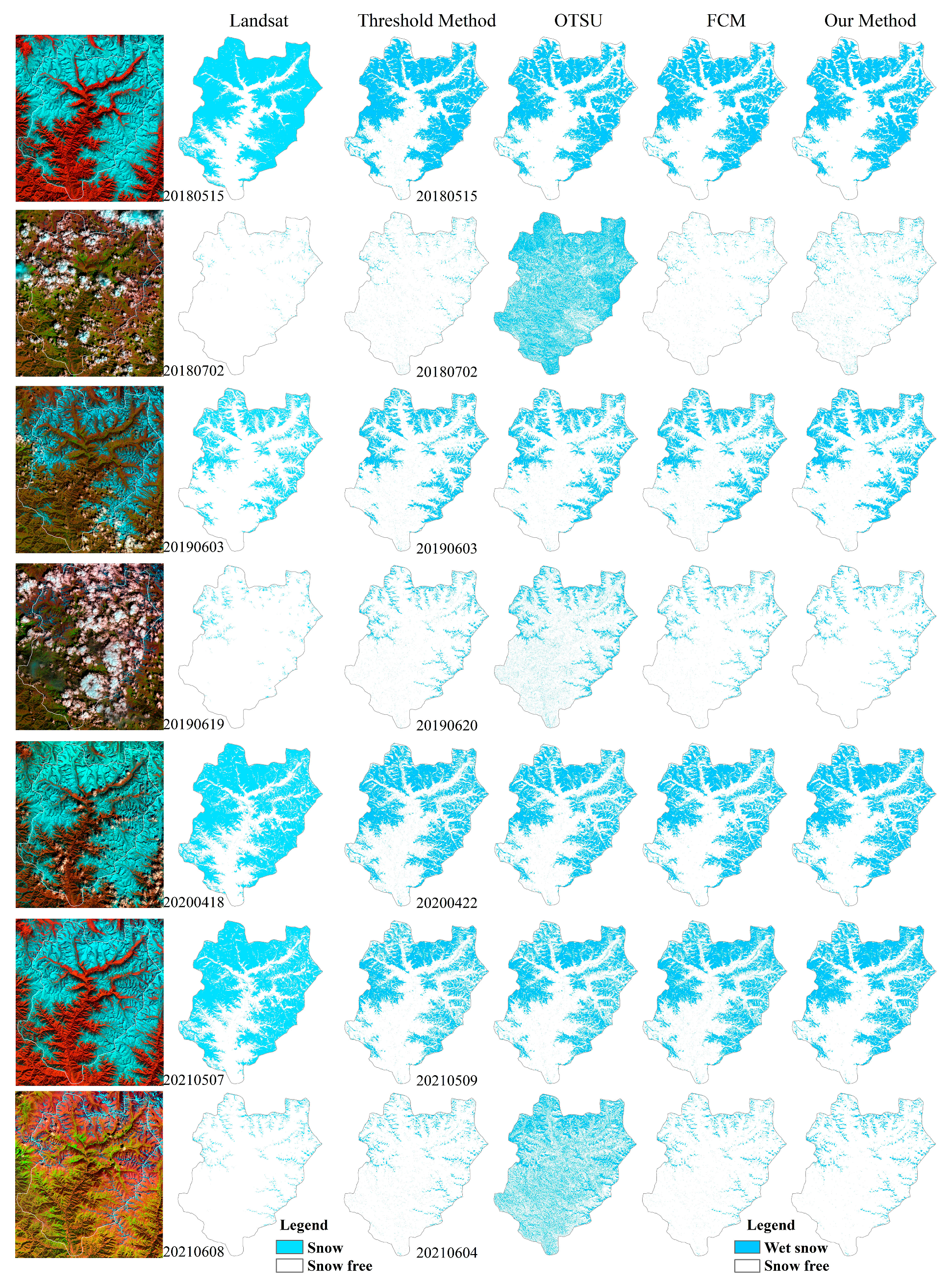
4.1. Comparison of Wet Snow Detection Accuracy Validation Results

Table 3. Comparison of wet snow extraction accuracy of different methods.

Sentinel-1 Date	Landsat Date	Method	Overall Accuracy/%	Precision/%	Recall/%	F1/%
15 May 2018	15 May 2018	Threshold Method	78.1	99.3	67.8	80.6
		OTSU	71.4	99.8	57.4	72.9
		FCM	72.0	99.8	58.4	73.7
		Our Method	72.8	99.8	59.6	74.6
2 July 2018	2 July 2018	Threshold Method	98.6	36.1	44.6	39.9
		OTSU	61.3	2.4	92.2	4.6
		FCM	98.7	38.9	39.4	39.1
		Our Method	97.3	22.6	65.9	33.6
3 June 2019	3 June 2019	Threshold Method	87.7	92.6	61.3	73.8
		OTSU	87.1	93.2	58.8	72.1
		FCM	87.7	92.6	61.3	73.8
		Our Method	89.7	90.0	71.7	79.8
20 June 2019	19 June 2019	Threshold Method	95.8	36.9	58.4	45.2
		OTSU	93.2	27.2	76.7	40.1
		FCM	96.1	38.7	53.1	44.8
		Our Method	96.2	39.6	53.2	45.4
22 April 2020	18 April 2020	Threshold Method	69.5	96.9	52.5	68.1
		OTSU	66.8	97.4	47.7	64.1
		FCM	68.7	97.1	60.0	66.9
		Our Method	71.5	96.9	55.7	70.7
9 May 2021	7 May 2021	Threshold Method	64.9	98.3	42.4	59.3
		OTSU	66.4	98.1	45.2	61.9
		FCM	69.0	97.6	49.7	65.9
		Our Method	71.9	97.2	55.0	70.3
4 June 2021	8 June 2021	Threshold Method	96.9	72.2	51.9	60.4
		OTSU	79.3	16.3	87.2	27.5
		FCM	96.0	54.5	65.6	59.6
		Our Method	96.7	63.9	63.6	63.8

Note: The bold text in the table represents the maximum values of wet snow detection accuracy results for the corresponding dates.

exhibits the stats of the wet snow extraction accuracy in the upper region of the Kayertes River Basin, comparing our method with the fixed-threshold method, OTSU algorithm, and FCM algorithm. The fixed-threshold method, which is commonly used for wet snow detection, was set to −3.5 dB for this region following comparative experiments. The OTSU method adjusts the threshold to maximize inter-class variance, optimizing wet snow detection, while the FCM method utilizes clustering to classify wet snow at the pixel level. According to Table 3, our method demonstrates superior accuracy for wet snow extraction, excluding for 2018. Calculating the average accuracy of the various methods across seven images during the snowmelt period,

Table 4. Average accuracy of wet snow extraction during the snowmelt period.

Method	Overall Accuracy/%	Precision/%	Recall/%	F1/%
Threshold Method	84.5	76.0	54.1	61.0
OTSU	75.1	62.1	66.5	49.0
FCM	84.0	74.2	55.4	60.5
Our Method	85.2	72.9	60.7	62.4

shows that our method achieves the highest average accuracy in wet snow detection, with an overall average of 85.2%. The fixed-threshold method is the second most accurate, while the OTSU algorithm shows the lowest accuracy.

Table 3 and Figure 5 show that on 22 April 2020 and 9 May 2021 the wet snow covered area was significantly large within the study region, and our method demonstrated higher accuracy with overall accuracy of 71.5% and 71.9%, respectively. Notably, on 9 May 2021, our method improved overall accuracy by approximately 7% compared to the fixed-threshold method. On 3 June 2019, as the wet snow area diminished, most of the snow in the basin was wet, and our method achieved an overall accuracy of 89.7%, outperforming the other methods by about 2%. During the late snowmelt periods of 2 July 2018, 20 June 2019, and 4 June 2021, when wet snow coverage was minimal, the accuracy of the three methods other than OTSU were similar. Toward the end of the snowmelt period, as the wet snow area decreased, the accuracy of our method and the threshold method gradually converge, with the threshold method showing relatively higher accuracy on 2 July 2018. Furthermore, on 15 May 2018, when wet snow covered about half of the study area, the histogram of the differential image displayed a bimodal distribution. Among the four methods, the fixed-threshold method had the highest extraction accuracy, with an overall accuracy of 78.1%, and the accuracy of the other three methods were similar on this date. Overall, across different snowmelt periods, the OTSU algorithm exhibited the lowest accuracy for wet snow extraction. During the mid-melt phase, our method showed better overall accuracy and F1 scores compared to the other methods, and various degrees of improvement in the accuracy of wet snow results extracted with our method.

From a spatial distribution perspective, Figure 5 shows that the wet snow ranges extracted using four methods are highly consistent with the results of optical data. However, the wet snow extents detected are relatively smaller compared to those identified in the Landsat images. Notably, compared to our method approach, the fixed-threshold method generates more “salt-and-pepper” noise in the extraction results. Additionally, our method effectively addresses issues of holes and fragmentation in the wet snow detection results as solar radiation and temperatures increase towards the end of the snowmelt period, leaving only small areas of wet snow in higher elevations. On 2 July 2018 and 4 June 2021, the OTSU algorithm, in particular, exhibited a significant number of misclassified pixels, markedly reducing its extraction accuracy.

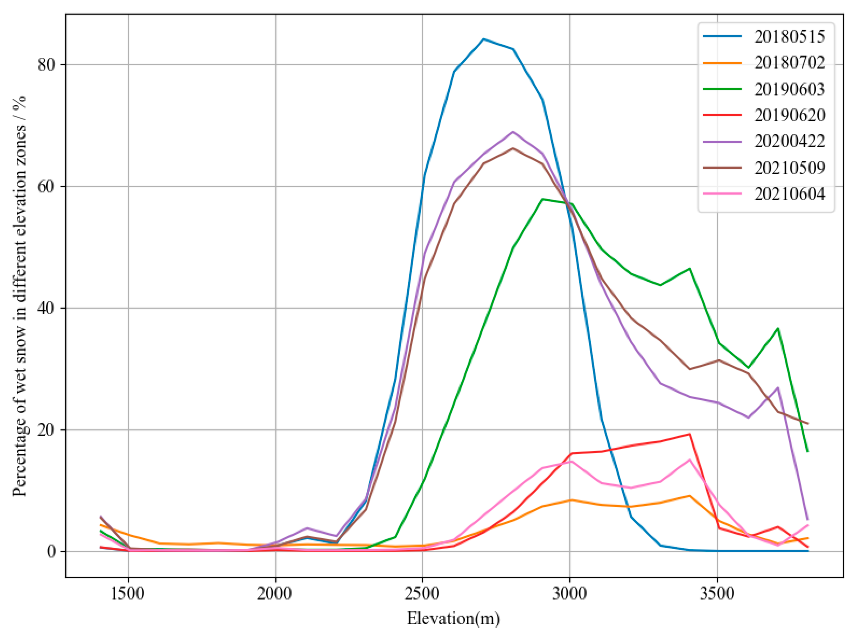
4.2. Wet Snow Cover Percentage across Various Elevation Zones

An analysis was conducted on the wet snow cover percentage across different elevation ranges with wet snow detection results. Elevations were segmented at 100 m intervals. Figure 6 shows that, during the mid-snowmelt period, the wet snow coverage increased significantly around an elevation of 2400 m, peaked between 2600 and 3000 m, and then decreased with higher elevations. The temperature in high-altitude areas is relatively low, and dry snow may exist in high-altitude areas [19], causing wet snow coverage to decrease. During the mid-snowmelt period, as the extent of wet snow decreased, a gradual reduction in wet snow percentage was observed below 3000 m, while an increase occurred at higher elevations, with the peak value of wet snow percentage gradually shifting to higher altitudes. This is consistent with the snow distribution and melting characteristics of high mountain areas during the mid-snowmelt phase; whereas snow at lower elevations melts and disappears early, substantial snow remains at mid to high elevations and gradually melts as it ascends [40,41]. At the end of the snowmelt period, the wet snow percentage began to increase around 2600 m and peaked between 3000 and 3500 m, showing a smaller wet snow percentage in each elevation zone. Overall, the wet snow extraction results and the sequence of snow melting across various elevations conform to general melting patterns.

Figure 6 highlights a significant difference in wet snow cover proportions at various elevations between 15 May 2018 and 22 April 2020. According to daily snow cover data, the coverage rates were 73% and 67%, respectively, with a notably smaller snow cover area on 22 April 2020. Additionally, ERA5-LAND data indicate that the daily average temperature was higher on 22 April 2020, suggesting that the melting process commenced earlier that year, which led to a pronounced melt period beginning in April. This variation is closely tied to both intra-annual and inter-annual temperature fluctuations, as well as the impacts of climate warming, indicating that the onset of wet snow melting varies annually, causing different degrees of melt.

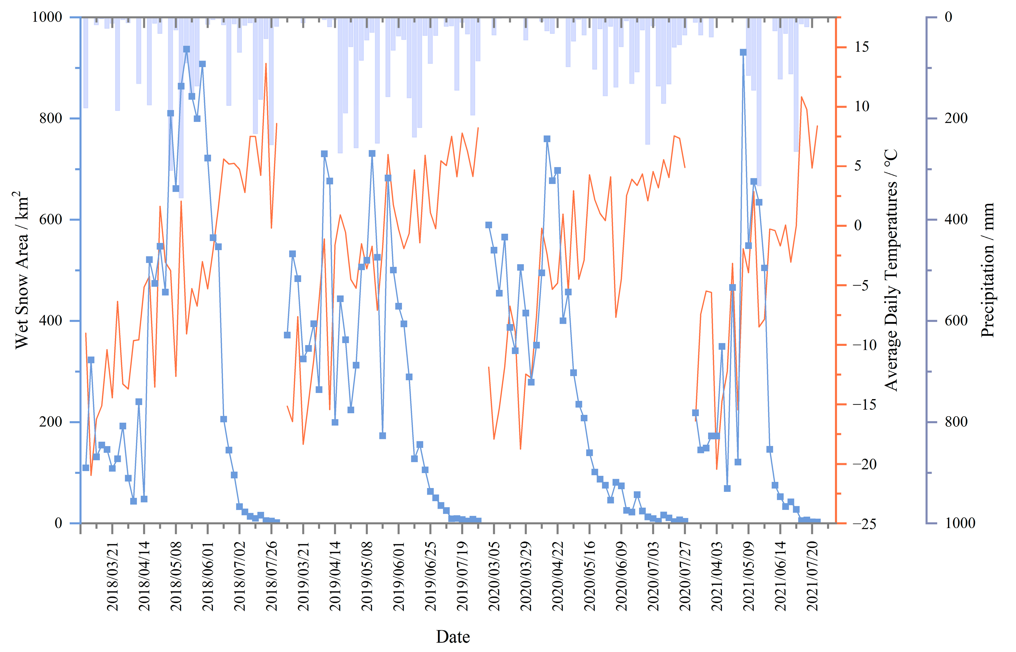
4.3. Temporal Characteristics of Wet Snow

Wet snow cover in the basin was extracted using data from Sentinel-1A and Sentinel-1B, spanning 136 temporal phases from March to July between 2018 and 2021. This extracted wet snow area was compared and analyzed with ERA5-Land daily average temperature and precipitation data, as shown in Figure 7.

During the snowmelt period, the area covered by wet snow initially increases and then decreases, with significant fluctuations observed in the early snow melting period in March and April. These changes in wet snow area correspond with trends observed in the ERA5-Land daily average temperature data. As temperatures rise in the middle of the snowmelt period, the coverage of wet snow gradually increases, and then gradually decreases towards the end of the melting period. The peak wet snow area in the high mountain regions for the years 2018 to 2021 occurred on 15 May, 10 May, 15 April, and 29 April, respectively. Zhou et al. [42] analyzed simulated monthly runoff data within the basin and found that annual runoff peaks typically occur between May and June, primarily due to snowmelt runoff. This finding is highly consistent with the larger wet snow areas observed in May and June. Accurate identification of wet snow distribution can enhance a model’s responsiveness to various hydrological characteristics, thereby improving the predictive accuracy of hydrological models in the basin.

Furthermore, there are differences in both inter-annual and intra-annual variations in wet snow area within the basin. In 2019, the intra-annual variation was particularly noticeable, with several peaks observed in April and May. ERA5-Land daily average temperature data shows significant temperature fluctuations during this period. Observations from optical imagery show an increase in snow cover from 3 May to 20 May, coinciding with a period of decreased temperatures and increased precipitation. This led to surface refreezing of the snowpack during Sentinel-1 satellite overpasses, resulting in a diminished wet snow area. Additionally, Sentinel-1A and Sentinel-1B pass over the basin at approximately 8 PM and 8 AM local time, respectively. During the early melt period, the large diurnal temperature variations cause surface melting and refreezing, resulting in substantial fluctuations in wet snow area.

5. Discussion

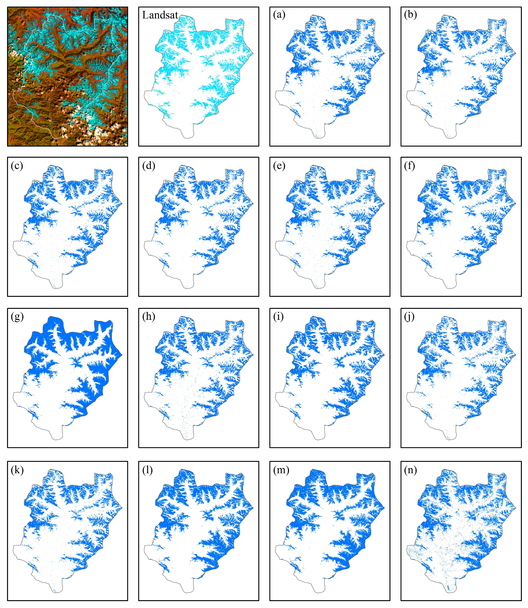
5.1. Differences in Wet Snow Detection Results with Different Data Combinations

Snow distribution is closely related to topographic features like elevation and slope. Building on previous research (e.g., Gallet et al. [20]), the combination of features has been shown to significantly enhance the robustness and accuracy of wet snow detection. This approach optimizes detection performance by leveraging the complementary strengths of each feature. Accordingly, in this study, various input data were selected to evaluate their impacts on wet snow detection results. The inputs include differential images, VV and VH polarizations backscatter information, elevation, and slope data, comprising a total of 14 data combinations detailed in

Table 5. Different combinations of input data.

Identifier	Channel Combinations
a	RC, RVV, RVH
b	RC, VVmelt, elevation
c	RC, VVmelt, slope
d	RC, VHmelt, elevation
e	RC, VHmelt, slope
f	RC, elevation, slope
g	VVmelt, VVsnow-free, elevation
h	VVmelt, VVsnow-free, slope
i	VVmelt, elevation, slope
j	VVmelt, VHsnow-free, elevation
k	VHmelt, VHsnow-free, slope
l	VHmelt, elevation, slope
m	VVmelt, VHmelt, elevation
n	VVmelt, VHmelt, slope

. These combinations are categorized into two groups: one focused on differential images (a–f) and the other on VV and VH polarizations backscatter coefficients (g–n). The average accuracy of wet snow detection was calculated across seven melt period scenes using various band combinations.

Table 6. Average accuracy of wet snow detection across seven melt period scenes with various band combinations.

	a	b	c	d	e	f	g	h	i	j	k	l	m	n
OA/%	84.2	83.6	85.2	84.8	84.8	84.4	78.3	84.5	80.6	81.4	83.6	80.6	82.3	79.7
F1/%	60.6	59.7	62.4	61.7	62.2	61.3	47.5	60.3	53.4	56.1	59.2	52.3	55.1	49.5

shows that the combination of differential images, VV polarization data, and slope information achieves the highest overall accuracy and F1 score in wet snow detection. Compared to backscatter data, differential images offer more stability and relatively higher accuracy in identifying wet snow. Using data from 3 June 2019, as an example, both qualitative and quantitative analyses were performed to evaluate the influence of different input data on wet snow detection results.

Various data combinations were input into the model for training, with the results of wet snow extraction for 3 June 2019 being shown in Figure 8 and the accuracy in Figure 9. Common wet snow detection methods are based on ratio or differential images, achieving a Kappa coefficient of 0.727 for wet snow extraction with differential images. Incorporating DEM elevation data reduced misclassification in lower elevation areas but introduced uncertainty in wet snow detection. This led to more fragmented distributions and increased misclassification at the edges of wet snow areas, ultimately decreasing accuracy. However, adding slope data improved accuracy, a finding consistent with the results of Gallet et al. [22]. Moreover, the inclusion of slope data proved more beneficial when using VV polarization backscatter information compared to VH polarization. When extracted with VV and VH polarizations data (Figure 8i,l), although areas not identified as wet snow based on differential images increased, the misclassification of other features such as shadows and lakes as wet snow also significantly increased, causing a rapid decline in precision. Overall, using differential images resulted in higher accuracy compared to backscatter information.

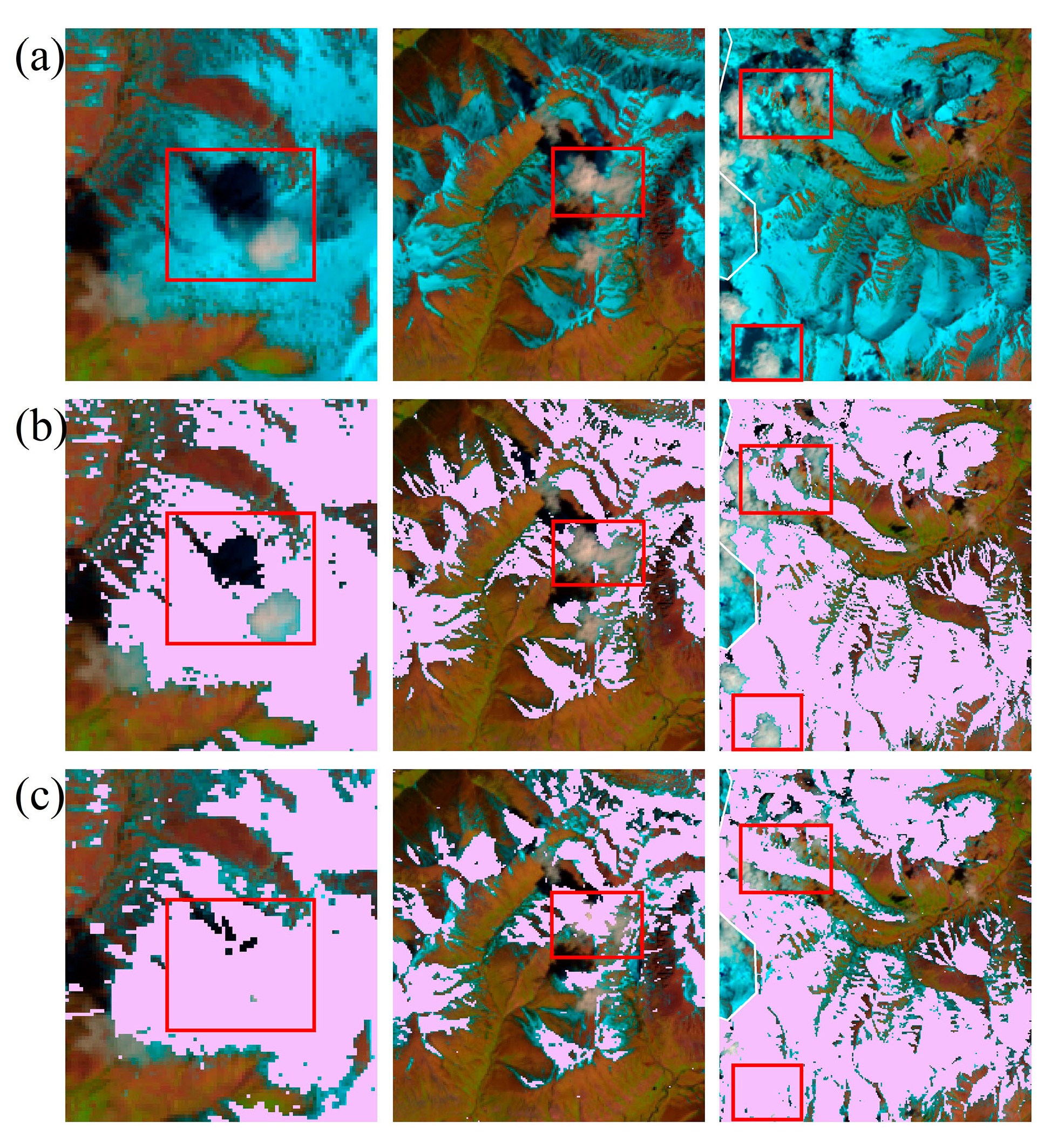
5.2. Under Cloud Wet Snow Detection

Cloud cover presents a significant challenge for snow cover detection using optical imagery, as it obscures visibility, making it difficult to identify snow under clouds [43]. Microwave remote sensing, which is unaffected by clouds, can complement the snow detection results derived from optical imagery. On 3 June 2019, during a period of intense snowmelt, most of the snow in the basin was wet. Figure 10 shows the use of optical imagery for false-color representation (Figure 10a) and the snow detection results with optical and microwave imagery, respectively (Figure 10b,c). As shown in Figure 10, in three cloud-covered areas, regions under cloud cover and cloud shadows were undetected in the optical imagery results (Figure 10b). Conversely, microwave data, as shown in Figure 10c, effectively extracted wet snow under clouds and cloud shadows, and accurately identified areas without snow under clouds. The application of microwave data can effectively improve the limitations of optical imagery, improving the accuracy of snow detection.

5.3. Uncertainties

We introduce a novel approach for wet snow detection that improves extraction accuracy during the mid-melt period compared to traditional threshold methods, though some uncertainties remain. As wet snow coverage decreases, increased misclassifications are observed in one of the three end-of-snowmelt images. While this method effectively suppresses point noise, it encounters limitations with block noise, leading to misclassifications. The detection results, influenced significantly by differential images, suggest that future studies could explore additional filtering techniques to mitigate noise and refine the processing of differential images based on wet snow characteristics. Such improvements could enhance the differentiation between wet snow and other surface features, thereby improving detection accuracy.

The validation of wet snow data using Landsat images introduces uncertainties. As temperatures rise, wet snow gradually melts to higher elevations [15,19]. During the early snowmelt period, snow at high altitudes may not have begun melting, and some areas may still contain dry snow. Sentinel-1′s C-band radar signals can penetrate several meters of dry snow and primarily detect wet snow, which leads to potential errors in high-altitude areas where dry snow predominates. Furthermore, there are uncertainties in identifying wet snow of low water content with SAR data. The Sentinel-1 satellite passes over the basin at 8 AM and 8 PM Beijing time. At these times, the surface of the wet snow may undergo a cycle of melting and refreezing, which increases volume scattering and consequently elevates the backscatter coefficient. This process can lead to inaccuracies in detecting wet snow with low water content. Additionally, the discrepancy in acquisition dates between Sentinel-1 and Landsat, particularly towards the end of the snowmelt period when wet snow melts rapidly, may cause inconsistencies in snow cover detection between the two datasets. Future research should incorporate more field data to further validate and refine remote sensing-based wet snow detection methods.

Additionally, the integration of the land-cover dataset revealed partial misclassifications in areas beneath forest, as well as in fragmented and edge regions of wet snow. In forested areas, C-band radar struggles to penetrate dense tree canopies, resulting in minimal differences in the backscatter coefficients under wet and dry snow conditions [44]. This similarity complicates the task of accurately mapping wet snow in such regions. The incorporation of InSAR coherence information, polarization parameters obtained from PolSAR polarization decomposition, can be considered in subsequent studies.

Finally, the side-looking geometry of the Sentinel-1 satellite results in phenomena such as layover and shadowing, leading to data gaps. While radiometric terrain correction using SRTM DEM data reduces these effects, some uncertainty persists. Moreover, differences in incidence angles between ascending and descending orbits can cause slight pixel mismatches. Although co-registration and geometric terrain correction have been applied, residual errors may remain. Sentinel-1A and Sentinel-1B satellites pass over the study area at approximately 8 AM and 8 PM local time, respectively. During early melt periods, diurnal temperature fluctuations can lead to snow melting and refreezing, which may affect backscatter signals and wet snow detection. To mitigate these uncertainties, future research could incorporate higher-resolution DEM data, apply interferometric coherence techniques, utilize polarization decomposition, and integrate meteorological data to enhance the accuracy and reliability of wet snow detection.

6. Conclusions

The main conclusions of this study are as follows:

(1)

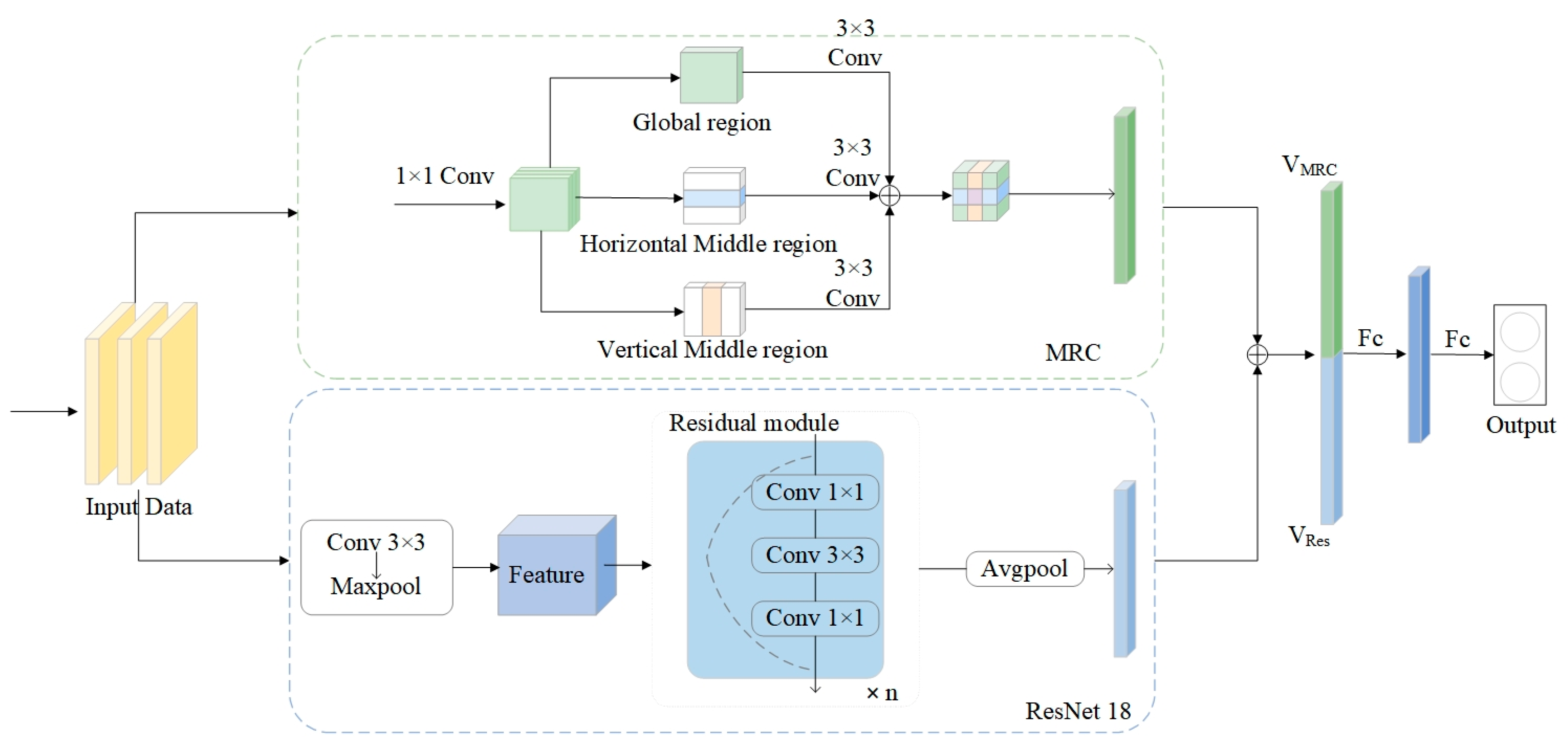
This study proposes a dual-branch deep learning model that incorporates a Multi-region Convolution module and ResNet18 for wet snow detection. This model operates within a weakly supervised classification framework and is distinguished by its capacity to autonomously learn complex features of wet snow, effectively utilize spatial neighborhood information, and reduce reliance on manual intervention. It can perform effective extraction in the absence of a large amount of labeled data.

(2)

The experiments showed that combinations of differential images, VV polarization data, and slope information provide advantages in wet snow extraction. Precision verification with optical imagery revealed that the average overall accuracy of wet snow detection in the study area was 85.2%. The overall accuracy of our method is particularly high when the proportion of wet snow cover is substantial.

References

1. Hammond, J.C.; Saavedra, F.A.; Kampf, S.K. Global snow zone maps and trends in snow persistence 2001–2016. Int. J. Climatol. 2018, 38, 4369–4383. [Google Scholar] [CrossRef]
2. Liu, Z.; Cuo, L.; Sun, N. Tracking snowmelt during hydrological surface processes using a distributed hydrological model in a mesoscale basin on the Tibetan Plateau. J. Hydrol. 2023, 616, 128796. [Google Scholar] [CrossRef]
3. Mankin, J.S.; Viviroli, D.; Singh, D.; Hoekstra, A.Y.; Diffenbaugh, N.S. The potential for snow to supply human water demand in the present and future. Environ. Res. Lett. 2015, 10, 114016. [Google Scholar] [CrossRef]
4. Che, T.; Hao, X.; Dai, L.; Li, H.; Huang, X.; Xiao, L. Snow Cover Variation and Its Impacts over the Qinghai-Tibet Plateau. Bull. Chin. Acad. Sci. 2019, 34, 1247–1253. [Google Scholar]
5. Jain, S.K.; Goswami, A.; Saraf, A.K. Snowmelt runoff modelling in a Himalayan basin with the aid of satellite data. Int. J. Remote Sens. 2010, 31, 6603–6618. [Google Scholar] [CrossRef]
6. Nagler, T.; Rott, H. Retrieval of wet snow by means of multitemporal SAR data. IEEE Trans. Geosci. Remote Sens. 2000, 38, 754–765. [Google Scholar] [CrossRef]
7. Dong, C. Remote sensing, hydrological modeling and in situ observations in snow cover research: A review. J. Hydrol. 2018, 561, 573–583. [Google Scholar] [CrossRef]
8. Dietz, A.J.; Kuenzer, C.; Gessner, U.; Dech, S. Remote sensing of snow–a review of available methods. Int. J. Remote Sens. 2012, 33, 4094–4134. [Google Scholar] [CrossRef]
9. Awasthi, S.; Varade, D. Recent advances in the remote sensing of alpine snow: A review. GIScience Remote Sens. 2021, 58, 852–888. [Google Scholar] [CrossRef]
10. Hao, X.; Huang, G.; Zheng, Z.; Sun, X.; Ji, W.; Zhao, H.; Wang, J.; Li, H.; Wang, X. Development and validation of a new MODIS snow-cover-extent product over China. Hydrol. Earth Syst. Sci. 2022, 26, 1937–1952. [Google Scholar] [CrossRef]
11. Hao, X.; Huang, G.; Che, T.; Ji, W.; Sun, X.; Zhao, Q.; Zhao, H.; Wang, J.; Li, H.; Yang, Q. The NIEER AVHRR snow cover extent product over China–a long-term daily snow record for regional climate research. Earth Syst. Sci. Data 2021, 13, 4711–4726. [Google Scholar] [CrossRef]
12. Riggs, G.A.; Hall, D.K. Reduction of cloud obscuration in the MODIS snow data product. In Proceedings of the 59th Eastern Snow Conference, Stowe, VT, USA, 5–7 June 2002; Volume 5. [Google Scholar]
13. Wang, X.; Han, C.; Ouyang, Z.; Chen, S.; Guo, H.; Wang, J.; Hao, X. Cloud–Snow Confusion with MODIS Snow Products in Boreal Forest Regions. Remote Sens. 2022, 14, 1372. [Google Scholar] [CrossRef]
14. Xiao, P.; Feng, X.; Xie, S.; Du, J. Research progresses of high-resolution remote sensing of snow in Manasi River Basin in Tianshan Mountains, Xinjiang Province. J. Nanjing Univ. (Nat. Sci.) 2015, 51, 909–920. [Google Scholar]
15. Darychuk, S.E.; Shea, J.M.; Menounos, B.; Chesnokova, A.; Jost, G.; Weber, F. Snowmelt characterization from optical and synthetic-aperture radar observations in the La Joie Basin, British Columbia. Cryosphere 2023, 17, 1457–1473. [Google Scholar] [CrossRef]
16. Tsai, Y.L.S.; Dietz, A.; Oppelt, N.; Kuenzer, C. Remote sensing of snow cover using spaceborne SAR: A review. Remote Sens. 2019, 11, 1456. [Google Scholar] [CrossRef]
17. Marin, C.; Bertoldi, G.; Premier, V.; Callegari, M.; Brida, C.; Hürkamp, K.; Tschiersch, J.; Zebisch, M.; Notarnicola, C. Use of Sentinel-1 radar observations to evaluate snowmelt dynamics in alpine regions. Cryosphere 2020, 14, 935–956. [Google Scholar] [CrossRef]
18. Nagler, T.; Rott, H.; Ripper, E.; Bippus, G.; Hetzenecker, M. Advancements for snowmelt monitoring by means of Sentinel-1 SAR. Remote Sens. 2016, 8, 348. [Google Scholar] [CrossRef]
19. Karbou, F.; Veyssière, G.; Coleou, C.; Dufour, A.; Gouttevin, I.; Durand, P.; Gascoin, S.; Grizonnet, M. Monitoring wet snow over an alpine region using Sentinel-1 observations. Remote Sens. 2021, 13, 381. [Google Scholar] [CrossRef]
20. Torralbo, P.; Pimentel, R.; Polo, M.J.; Notarnicola, C. Characterizing snow dynamics in semi-arid mountain regions with multitemporal Sentinel-1 imagery: A case study in the Sierra Nevada, Spain. Remote Sens. 2023, 15, 5365. [Google Scholar] [CrossRef]
21. Liu, C.; Li, Z.; Zhang, P.; Wu, Z. Seasonal snow cover classification based on SAR imagery and topographic data. Remote Sens. Lett. 2022, 13, 269–278. [Google Scholar] [CrossRef]
22. Gallet, M.; Atto, A.; Karbou, F.; Trouvé, E. Wet snow detection from satellite SAR images by machine learning with physical snowpack model labelling. IEEE J. Sel. Top. Appl. Earth Obs. Remote Sens. 2023, 17, 2901–2917. [Google Scholar] [CrossRef]
23. Qu, X.; Gao, F.; Dong, J.; Du, Q.; Li, H. Change detection in synthetic aperture radar images using a dual-domain network. IEEE Geosci. Remote Sens. Lett. 2021, 19, 4013405. [Google Scholar] [CrossRef]
24. Shafique, A.; Cao, G.; Khan, Z.; Asad, M.; Aslam, M. Deep learning-based change detection in remote sensing images: A review. Remote Sens. 2022, 14, 871. [Google Scholar] [CrossRef]
25. Du, Y.; Zhong, R.; Li, Q.; Zhang, F. TransUNet++ SAR: Change detection with deep learning about architectural ensemble in SAR images. Remote Sens. 2022, 15, 6. [Google Scholar] [CrossRef]
26. Wang, Y.; Su, J.; Zhai, X.; Meng, F.; Liu, C. Snow coverage mapping by learning from Sentinel-2 satellite multispectral images via machine learning algorithms. Remote Sens. 2022, 14, 782. [Google Scholar] [CrossRef]
27. Wang, Z.; Fan, B.; Tu, Z.; Li, H.; Chen, D. Cloud and snow identification based on DeepLab v3+ and CRF combined model for GF-1 WFV images. Remote Sens. 2022, 14, 4880. [Google Scholar] [CrossRef]
28. Yang, J.; Li, W.; Chen, K.; Liu, Z.; Shi, Z.; Zou, Z. Weakly supervised adversarial training for remote sensing image cloud and snow detection. IEEE J. Sel. Top. Appl. Earth Obs. Remote Sens. 2024, 17, 15206–15221. [Google Scholar] [CrossRef]
29. Zhang, W.; Shen, Y.; Wang, N.; He, J.; Chen, A.; Zhou, J. Investigations on physical properties and ablation processes of snow cover during the spring snowmelt period in the headwater region of the Irtysh River, Chinese Altai Mountains. Environ. Earth Sci. 2016, 75, 199. [Google Scholar] [CrossRef]
30. Zhang, W.; Shen, Y.; He, J.; He, B.; Wu, X.; Chen, A.; Li, H. Assessment of the effects of forest on snow ablation in the headwaters of the Irtysh River, Xinjiang. J. Glaciol. Geocryol. 2014, 36, 1260–1270. [Google Scholar]
31. Wu, X.; Zhang, W.; Li, H.; Long, Y.; Pan, X.; Shen, Y. Analysis of seasonal snowmelt contribution using a distributed energy balance model for a river basin in the Altai Mountains of northwestern China. Hydrol. Process. 2021, 35, e14046. [Google Scholar] [CrossRef]
32. Wu, X.; Pan, X.; Shen, Y.; Zhang, W.; He, J.; He, B. Validation of WRF model on simulating forcing data for Kayiertesi River basin, Xinjiang. J. Glaciol. Geocryol. 2016, 38, 332–340. [Google Scholar]
33. Hall, D.K.; Riggs, G.A.; Salomonson, V.V. Development of methods for mapping global snow cover using moderate resolution imaging spectroradiometer data. Remote Sens. Environ. 1995, 54, 127–140. [Google Scholar] [CrossRef]
34. Snapir, B.; Momblanch, A.; Jain, S.K.; Waine, T.W.; Holman, I.P. A method for monthly mapping of wet and dry snow using Sentinel-1 and MODIS: Application to a Himalayan river basin. Int. J. Appl. Earth Obs. Geoinf. 2019, 74, 222–230. [Google Scholar] [CrossRef]
35. Gao, F.; Dong, J.; Li, B.; Xu, Q. Automatic change detection in synthetic aperture radar images based on PCANet. IEEE Geosci. Remote Sens. Lett. 2016, 13, 1792–1796. [Google Scholar] [CrossRef]
36. He, K.; Zhang, X.; Ren, S.; Sun, J. Deep residual learning for image recognition. In Proceedings of the IEEE Conference on Computer Vision and Pattern Recognition, Las Vegas, NV, USA, 27–30 June 2016. [Google Scholar]
37. Otsu, N. A threshold selection method from gray-level histograms. Automatica 1975, 11, 285–296. [Google Scholar] [CrossRef]
38. Bezdek, J.C.; Ehrlich, R.; Full, W. FCM: The fuzzy c-means clustering algorithm. Comput. Geosci. 1984, 10, 191–203. [Google Scholar] [CrossRef]
39. Rondeau-Genesse, G.; Trudel, M.; Leconte, R. Monitoring snow wetness in an Alpine Basin using combined C-band SAR and MODIS data. Remote Sens. Environ. 2016, 183, 304–317. [Google Scholar] [CrossRef]
40. Tang, Z.; Deng, G.; Hu, G.; Wang, X.; Jiang, Z.; Sang, G. Spatiotemporal dynamics of snow phenology in the High Mountain Asia and its response to climate change. J. Glaciol. Geocryol. 2021, 43, 1400–1411. [Google Scholar]
41. Tang, Z.; Deng, G.; Hu, G.; Zhang, H.; Pan, H.; Sang, G. Satellite observed spatiotemporal variability of snow cover and snow phenology over high mountain Asia from 2002 to 2021. J. Hydrol. 2022, 613, 128438. [Google Scholar] [CrossRef]
42. Zhou, G.; Zhao, Q.; Zhang, S.; Zhang, D.; Li, C. Rolling forecast of snowmelt floods in data-scarce mountainous regions using weather forecast products to drive distributed energy balance hydrological model. J. Hydrol. 2024, 637, 131384. [Google Scholar] [CrossRef]
43. Li, X.; Jing, Y.; Shen, H.; Zhang, L. The recent developments in cloud removal approaches of MODIS snow cover product. Hydrol. Earth Syst. Sci. 2019, 23, 2401–2416. [Google Scholar] [CrossRef]
44. Baghdadi, N.; Gauthier, Y.; Bernier, M. Capability of multitemporal ERS-1 SAR data for wet-snow mapping. Remote Sens. Environ. 1997, 60, 174–186. [Google Scholar] [CrossRef]
Figure 1. Study area. (a) Elevation. (b) Land-cover types.
Remotesensing 16 03575 g001
Figure 2. Differential images and corresponding histograms for different snow melting periods in 2019.
Remotesensing 16 03575 g002
Figure 3. (a) Landsat image from 2 July 2018. (b) HFCM clustering results with an initial cluster number of 5. (c) HFCM clustering results with an initial cluster number of 2.
Remotesensing 16 03575 g003
Figure 4. Architecture of the dual-branch deep learning model. n is the number of residual blocks and different values are chosen depending on the neighbourhood size. When the neighbourhood size is 7, n = 3.
Remotesensing 16 03575 g004
Figure 5. Wet snow extraction results of the four methods.
Remotesensing 16 03575 g005
Figure 6. Wet snow percentage across different elevation zones.
Remotesensing 16 03575 g006
Figure 7. Wet snow cover area, temperature, and precipitation from March to July 2018–2021.
Remotesensing 16 03575 g007
Figure 8. Wet snow detection results with different input data on 3 June 2019. (an) correspond to the identification results of different band combinations in Table 5.
Remotesensing 16 03575 g008
Figure 9. Comparison of wet snow extraction accuracy with different input data.
Remotesensing 16 03575 g009
Figure 10. Snow detection under cloud cover. (a) Landsat false-color image. (b) Optical imagery detection results. (c) Wet snow detection results.
Remotesensing 16 03575 g010