Recent Patterns and Trends of Snow Cover (2000–2023) in the Cantabrian Mountains (Spain) from Satellite Imagery Using Google Earth Engine

Abstract

Snow cover is a relevant component of the Earth’s climate system, influencing water supply, ecosystem health, and natural hazard management. This study aims to monitor daily snow cover in the Cantabrian Mountains using Sentinel-2, Landsat (5–8), and MODIS data processed in Google Earth Engine (GEE). The main purpose is to extract metrics on snow cover extent, duration, frequency, and trends. Key findings reveal significant spatial and temporal variability in Snow-Cover Days (SCDs) across the region. Over the past 23 years, there has been a notable overall decrease in snow-cover days (−0.26 days per year, and −0.92 days per year in areas with a significant trend). Altitudes between 1000–2000 m a.s.l. showed marked decreases. The analysis of Snow-Cover Fraction (SCF) indicates high interannual variability and records the highest values at the end of January and the beginning of February. The effectiveness of satellite data and GEE is highlighted in providing detailed, long-term snow cover analysis, despite some limitations in steep slopes, forests, and prolonged cloud-cover areas. These results underscore the capacity for continuous monitoring with satellite imagery, especially in areas with sparse snow observation networks, where studies could be enhanced with more localized studies or additional ground-based observations.

1. Introduction

Snow cover in mountainous regions is critically important for several reasons. Hydrologically, snow acts as a natural reservoir, gradually releasing water and maintaining river flows during the spring and summer months, which is crucial for water supply and ecosystem health [1,2,3]. Snow also poses a significant natural hazard, with extreme snowfall events causing material, infrastructural, and even personal damage [4,5]. Additionally, avalanches impact communication networks and accessibility [6,7]. In the areas influenced by the Mediterranean climate, mountainous regions experience high seasonal and interannual snow distribution variability [8] and are also affected by drought episodes [9], rain-on-snow events [10,11,12,13], or dust deposition from the Sahara Desert on the snowpack [14,15,16]. Moreover, global change scenarios foresee changes in the river regimes dependent on the mountains of Mediterranean environments, which are experiencing changes in snow accumulation and melt patterns [17,18,19,20].

On the other hand, snow is one of the 55 Essential Climate Variables (ECVs) defined by the Global Climate Observing System (GCOS) of the World Meteorological Organization (WMO) [21,22]. The detection of snow cover using satellite imagery has become increasingly effective with the advent of remote sensing technologies [23,24,25]. Remote sensing provides a powerful tool for continuous and large-scale monitoring of snow dynamics, offering valuable data for hydrological modelling, climate studies, and natural hazard management [26,27,28]. Multispectral satellite images with daily or weekly temporal resolution enable the monitoring of changes in snow cover through the calculation of spectral indices, such as the Normalized Difference Snow Index (NDSI) [29,30,31]. As a main limitation, the quality and availability of data in passive sensors vary spatially and temporally due to factors associated with cloudiness [32]. Additionally, snow-cover detection with satellite in forested areas is constrained [33,34,35,36]. Low NDSI values are obtained in forested areas, as it does not identify snow beneath the forest canopy [24].

Google Earth Engine (GEE) has emerged as a key tool for large-scale processing of satellite imagery [37,38,39,40]. Its cloud-based platform allows researchers to access, process, and analyse satellite data at unprecedented scales and speeds. For snow-cover studies, GEE facilitates the integration of various datasets, application of algorithms, and generation of time-series analyses, significantly enhancing the efficiency and scope of snow monitoring efforts [41,42,43]. This capability is particularly valuable for tracking trends in snow cover over time, assessing seasonal variations, and understanding the impacts of climatic shifts [44].

Tools for extracting statistics on snow dynamics have been developed with Google Earth Engine in recent years, which has enabled the implementation of several interactive viewers that facilitate the extraction of snow-cover duration statistics. The tool “SnowWarp”, developed in R by Laurin et al. [45], calculates maps of fractional and binary snow-covered area (fSCA and bSCA) for extracting the dates of the beginning and end of the snow season, as well as the number of annual Snow-Cover Days (SCDs). This was carried out for the period 2000–2021 with a spatial resolution of 30 m globally by combining MODIS and Landsat images. Gascoin et al. [46] provided a web application to monitor, in real time, the snow-cover state in the Alps through a 30-year snow cover time-series based on satellite (MODIS) and reanalysis data. SnowCloudMetrics [47] is a web portal based on the MOD10A1 dataset (Terra Snow Cover Daily Global 500 m) which extracts Snow-Cover Frequency (SCF) and the Day of Snow Disappearance (SDD) by hydrological year between 2001 and 2019 globally. Based on this, SnowCloudHydro [48] uses SnowCloudMetrics as a key model input to extract monthly SCFs for a quicker and more optimized basin hydrologic modelling. El jabiri et al. [49] recorded Sentinel-2 and Landsat-8 snow-cover metrics in the Moroccan Atlas Mountains in recent years using Google Earth Engine, focusing on the duration of snow cover and obtaining a high agreement with in situ data observations.

The Cantabrian Mountains extend approximately 300 km longitudinally in northern Spain, forming a natural barrier between the Cantabrian Sea and the Spanish Northern Plateau (Figure 1). This region is distinguished by significant structural variations, resulting in a pronounced asymmetry between the slopes. The climate exhibits considerable variability, contributing to a rich diversity of landscapes. On the northern slope, an oceanic climate with a steep altitudinal gradient prevails, while the southern slope features a transition towards sub-Mediterranean and sub-Atlantic climates with a gentler altitudinal gradient and frequent snowfalls [50]. Mean annual precipitation ranges from 800 to over 2000 mm, displaying significant asymmetry, with higher amounts observed on the northern slope as well as at the eastern and western extremes. The southern slope experiences greater continentality and insolation. Prominent peaks within this range, including the Picos de Europa, Fuentes Carrionas Massif, Peña Ubiña Massif, Sierra de Híjar, Mampodre Massif, and Sierra de Gistredo, rise above 2000 m, with Torre Cerredo in the Picos de Europa reaching an elevation of 2650 m.

Recent climatic and geomorphological studies have highlighted the local importance of snow cover in high-altitude areas of the Cantabrian Mountains [51]. Snowfall events in the Cantabrian Mountains can be intense, sometimes causing personal [52] or material damage, often because of avalanches, which are also an important element in the landscape dynamics [53,54,55,56,57]. Findings indicate significant interannual variability in snow-cover duration [58] and a regressive trend in snow cover since the mid-20th century in the western range [55], the northern slope [54], and the southern slope of the Cantabrian Mountains [59,60]. Snow plays a significant role in the thermal regime of the soil and the geomorphological dynamics of high areas of the Cantabrian Mountains [53,58,61,62,63]. Hence, the monitoring of snow cover using satellite imagery can be a highly valuable complement to these studies, providing detailed data on local snow distribution patterns in areas with a scarcity of snowpack observations [63,64,65].

The aim of this article is to present the snow-cover distribution and trends in Snow-Cover Days by leveraging a wide range of available satellite data (Sentinel-2, Landsat 5, Landsat 8, and MODIS) and the capabilities of Google Earth Engine. From this, statistical metrics on the extent, duration, frequency, and trends of snow cover are extracted for the Cantabrian Mountains area.

2. Materials and Methods

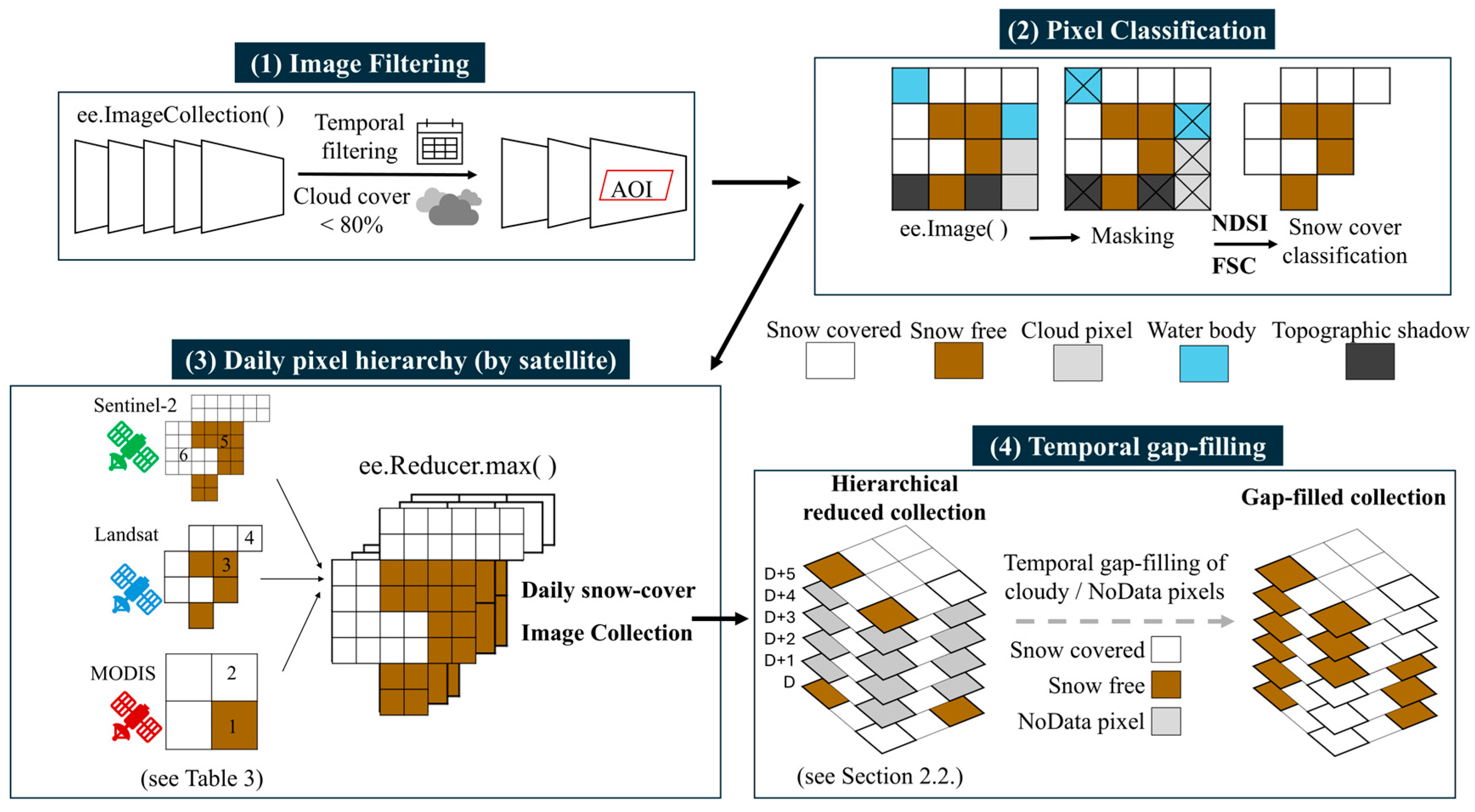
2.1. Creation of Daily Snow Cover Image Collection

The processing and extraction of daily snow-cover images in the Cantabrian Mountains have been performed using multiple Google Earth Engine products (

Table 1. Description of satellite products used in Google Earh Engine (GEE).

Google Earth Engine Product	Satellite	Temporal Resolution	Spatial Resolution	Dataset Availability	Number of Images
Harmonized Sentinel-2 MSI: MultiSpectral Instrument, Level-2A	Sentinel-2A Sentinel-2B	5 days	10, 20, 60 m	2015–present	4349
USGS Landsat 5 Level 2, Collection 2, Tier 1	Landsat-5	16 days	30 m (TM bands)	1984–2012	514
USGS Landsat 8 Level 2, Collection 2, Tier 1	Landsat-8	16 days	15, 30, 100 m	2013–present	1101
MOD10A1.061 Terra Snow Cover Daily Global 500 m	Terra-MODIS	Daily	250, 500, 1000 m	1999–present	4867

), facilitating the massive processing of a large number of cloud-based images. Thus, a total of 10,831 satellite images were used: 4349 images from Sentinel 2-A and Sentinel 2-B from granules 29TPJ, 29TPH, 29TQJ, 29TQH, 30TUP, 30TVP, 30TUN, and 30TVN. In addition, 514 images from Landsat-5 and 1101 images from Landsat-8 were used from the WRS-2 Path/Row 203/30, 202/30, and 201/30. Neither Sentinel or Landsat cover the entire extent of the Cantabrian Mountains in a single image. In the case of MODIS, the images provide total coverage, so 4867 images were used after discarding those with more than 80% cloud cover in the study area.

The workflow (Figure 2) shows multiple phases for extracting the snow-cover image collection. Initially, the first phase involves image collection filtering and pixel masking. The collections have been filtered according to three criteria for image selection: temporal filtering for the period of 2000–2024, spatial filtering according to the Area of Interest (AOI), the Cantabrian Mountains, and finally, images with more than 80% cloud cover within the study area are filtered and excluded. Subsequently, pixel masking is performed to remove unwanted pixels from the selected images, such as water bodies. Larger water bodies (reservoirs) are manually masked in the analysis using a layer from the inventory of reservoirs in Spain (https://datos.gob.es/es/catalogo/e05068001-inventario-de-presas-y-embalses, accessed on 31 July 2024) loaded in Google Earth Engine as an Asset. For other water bodies, they are removed using a mask with the Normalized Difference Water Index (NDWI), calculated from the Green and NIR bands, masking values greater than 0.3. In case of topographic shadows, they have only been removed in Sentinel-2 using the Scene Classification Layer (SCL) by removing the topographically cast shadows (value = 2). Other SCL values are used to mask clouds (values = 3, 8, 9, 10). In the case of Landsat 5 and 8, cloud cover is masked using the QA_PIXEL Bitmask, with Bit 3 for clouds and Bit 4 for cloud shadows. Topographic shadows have not been corrected in Landsat images.

The second phase is the classification of pixels as snow-covered and snow-free on each image source. For this, two different methods were used depending on the satellite platform. For the Landsat and Sentinel satellites, the Normalized Difference Snow Index (NDSI) [29,30,31] was used, with an NDSI threshold of >0.4 used to define areas covered by snow.

$$\mathrm{Normalized} \mathrm{Difference} \mathrm{Snow} \mathrm{Index} (\mathrm{NDSI})={\displaystyle \frac{(Green-SWIR)}{(Green+SWIR)}}$$

This index exploits the distinct reflective properties of snow in the visible (green) and the shortwave infrared wavelengths (SWIR) (

Table 2. Green and SWIR band specifications for Sentinel-2, Landsat-5, Landsat-8, and MODIS.

Satellite	Green Band	Green Band Wavelength	SWIR Band	SWIR Band Wavelength
Sentinel-2	B3	560 nm	B11	1610 nm
Landsat-5	B2	520–600 nm	B5	1550–1750 nm
Landsat 8	B3	530–590 nm	B6	1570–1650 nm
MODIS	B4	545–565 nm	B6	1628–1652 nm

) to identify snow-covered areas.

For snow-cover extraction with MODIS, the ‘NDSI_Snow_cover’ band was used, making a transformation to Fractional Snow Cover (FSC), based on Salomonson and Appel [66] and Rittger et al. [67]

Fractional Snow Cover (FSC): −0.01 + 1.45 × NDSI

Thus, pixels with values higher than FSC > 0.15 were classified as snow-covered, referencing partially and fully covered areas in the study by Revuelto et al. [68], based on the threshold estimations in the Picos de Europa area.

The results of the snow classifications with each satellite lead to one to three daily snow classifications for some parts of the Cantabrian Mountains. Given its length of about 300 km, the swath widths of Landsat and Sentinel cannot cover the entire study area. On a daily level, since February 2000, Terra’s MODIS product has covered the entire Cantabrian Mountains with a spatial resolution of 500 m. In cases where two or all three satellites capture images of the same sector of the range on the same day, images with higher spatial resolution are prioritised (Sentinel > Landsat > MODIS). Values have been reclassified with numerical values from 6 to 1 (

Table 3. Reclassification values assigned to snow-covered and snow-free pixels.

Satellite	Snow Covered	Snow Free
Sentinel	6	5
Landsat	4	3
MODIS	2	1

).

Using a reducer, the maximum daily value for each pixel is calculated, prioritising the classification of both snow-covered and snow-free pixels for satellites with lower spatial resolution (Figure 3). The reducer uses the ee.Reducer.max() function from Google Earth Engine, thereby selecting the highest pixel value from the hierarchy and discarding the rest. This helps to avoid overlapping snow-cover classifications on the same day, in case two satellites (with two different spatial resolutions) coexist in the same area. The spatial resolution is, therefore, variable in the snow classification for the same day, depending on the satellite with the best available spatial resolution. Snow-cover pixels classified from Sentinel-2 will have a resolution of 20 m, which is the highest spatial resolution, while those classified with MODIS will have a resolution of 500 m.

2.2. Data Gap-Filling Due to Cloud Cover

The main limitation in snow-cover detection arises due to cloud cover, which is particularly common on the northern slopes of the Cantabrian Mountains and can persist for several consecutive days, especially during snowfall episodes. Thus, the number of images used in this study for each pixel varies depending on the location, being lower in areas with higher cloud cover (Figure 4).

Consequently, the update of the snow-cover extent usually occurs with a few days’ delay, provided the snow cover remains until the first cloud-free pass of one of the satellites. To address this fact, a temporal gap-filling has been performed, applying temporal gap-filling with linear interpolation as described in Sproles et al. [48]. Considering the average consecutive cloud cover in the Cantabrian Mountains (adding map made with MODIS), the maximum data filling period threshold has been set to 5 days, thus covering most episodes of continuous cloud cover, with an average duration of 3.3 consecutive days for the entire Cantabrian Mountains, calculated from daily MODIS images for the period of 2000–2023. Gap-filling is performed using the following conditions (see Figure 2):

• If an image D − i has snow, D has no data (cloud), and D + i has snow → D is classified as snow.
• If an image D − i is snow-free, D has no data (cloud), and D + i is snow-free → D is classified as snow-free.
• If an image D − i is snow-free, D has no data (cloud), and D + i has snow → D is classified as snow. D is classified as snow from the day when the simple interpolation of NDSI or FSC values from the last available data to the first available data after the gap indicates snow presence.
• If an image D − i is snow-covered, D has no data (cloud), and D + i is snow-free → D is classified as snow. D is classified as snow from the day when the simple interpolation of NDSI or FSC values from the last available data to the first available data after the gap indicates snow presence.

The “i” value ranges from 1 day up to a maximum of 3 days, to reach a maximum period of gap-filling of 5 days. This has been established according to the mode of continuous cloud-cover days, which is higher on the northern slope of the study area. In cases where there are no data due to gaps of more than 5 consecutive days of cloud cover, the pixel is classified as NoData during the cloud-cover period, as there is no nearby temporal evidence to classify it as either snow-covered or snow-free. The pixel remains as NoData until the next available cloud-free image.

2.3. Extraction of Snow-Cover Days (SCDs) and Snow-Cover Fraction (SCF) Statistics

All the aforementioned steps (image filtering, unwanted pixel masking, and snow-covered and snow-free zone classification) and temporal gap-filling result in a daily image collection of snow-covered areas. From this collection, some statistics have been derived.

Firstly, the statistics related to snow-cover frequency were calculated for each pixel to extract the average annual duration and its trends:

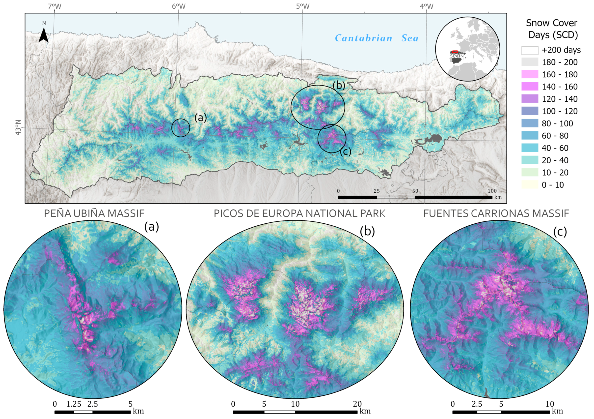
• Snow-Cover Days (SCDs): for each pixel, the calculation of the number of images where the pixel is snow-covered divided by the total number of valid (cloud-free) images, multiplied by 365. Calculations are made for the period from October 2000 to September 2023 and values can range between 0 and 365 days of snow cover.
• Annual Snow-Cover Days (aSCDs): for each season (October—September), the same calculation as SCDs. This statistic is used to calculate trends. Values can range between 0 and 365 days.
• Trends in Snow-Cover Days: Sen’s slope test [69] is applied to annual SCDs to assess the magnitude and direction of the trend over time in a yearly scale. Additionally, the Mann–Kendall test [70,71] is employed at a 95% confidence level to determine the significance of these trends. Absolute and relative trend is calculated. The absolute trend refers to the number of days per year that the SCDs changes (a −0.5 value means it decreases by 0.5 days each year, or 5 days every 10 years). In contrast, the relative trend is calculated considering the average SCDs for each pixel, resulting in a percentage value (a −0.5 value of relative trend means that the snow cover decreases by 0.5% from the average snow cover value at that point each year, or by 5% every 10 years).

Sentinel-2 images (recorded only since 2015) have not been used in trend analysis to avoid disruptions in the frequency of sub-pixel snow-cover observations, as this was problematic in pixels with high topographic variability.

Secondly, calculations were performed to evaluate the total extent of the range that was covered by snow, using the Snow-Cover Fraction (SCF):

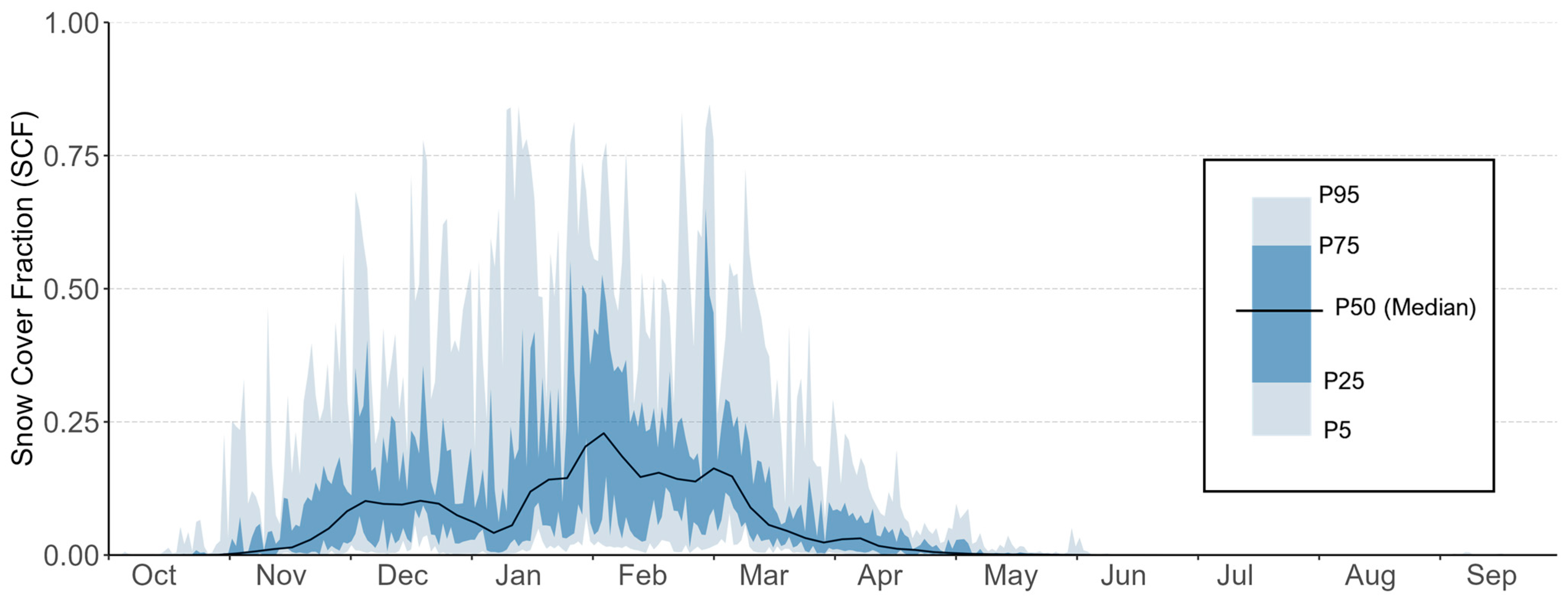
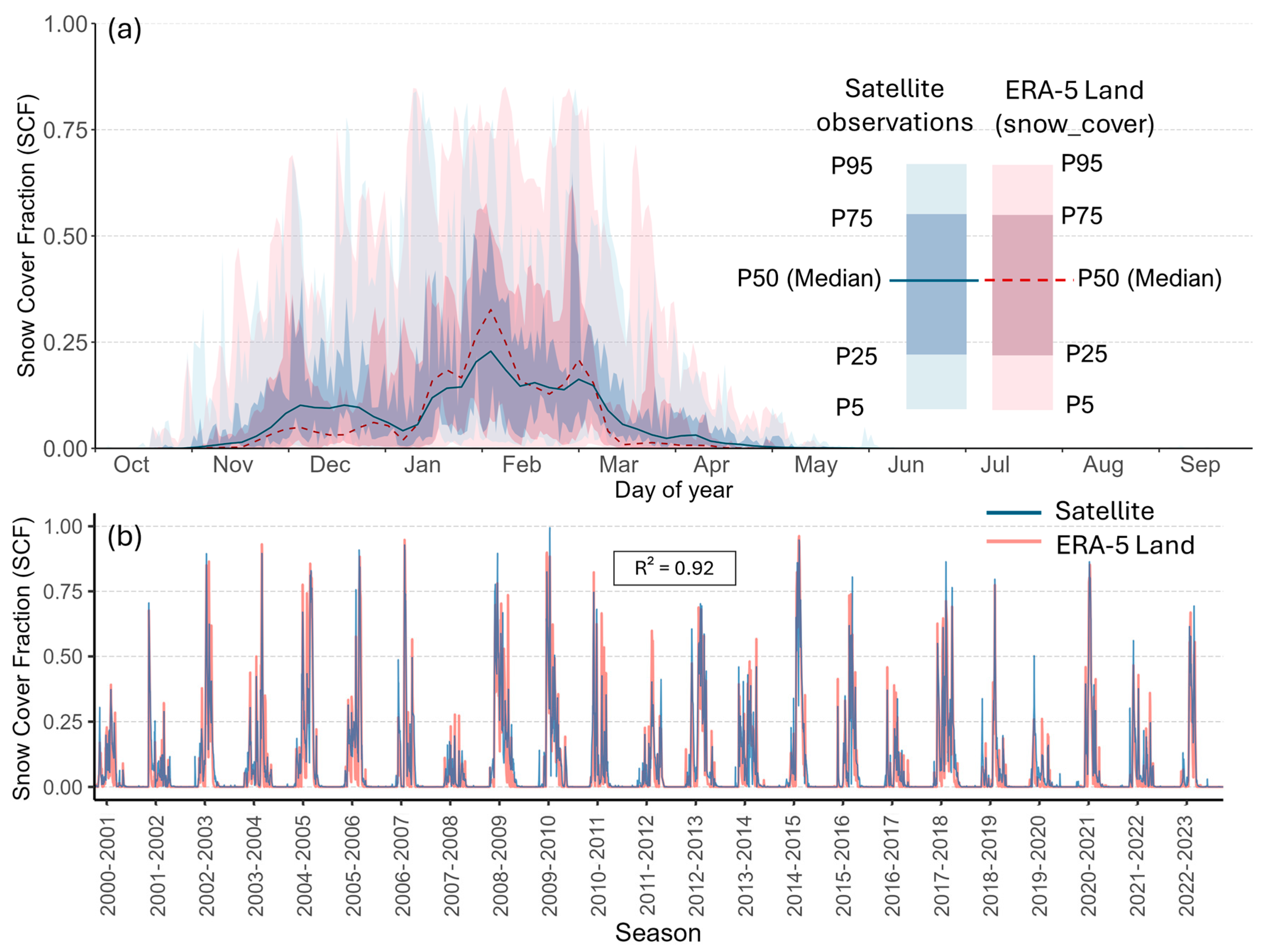
• Snow-Cover Fraction (SCF): for the entire Cantabrian Mountains, the daily calculation of the number of snow-covered pixels/total number of available pixels (cloud-free) in the area. Values can vary daily between 0 and 1, being zero when no area of the valid (cloud-free) pixels are covered by snow and one when, on a specific day, all valid (cloud-free) pixels are snow-covered. Satellite values will be compared with the SCF records of the ‘snow_cover’ variable data from the ERA5-Land climate reanalysis product [72], although it is important to note that it is a product with a resolution of 0.1° (11,132 m).
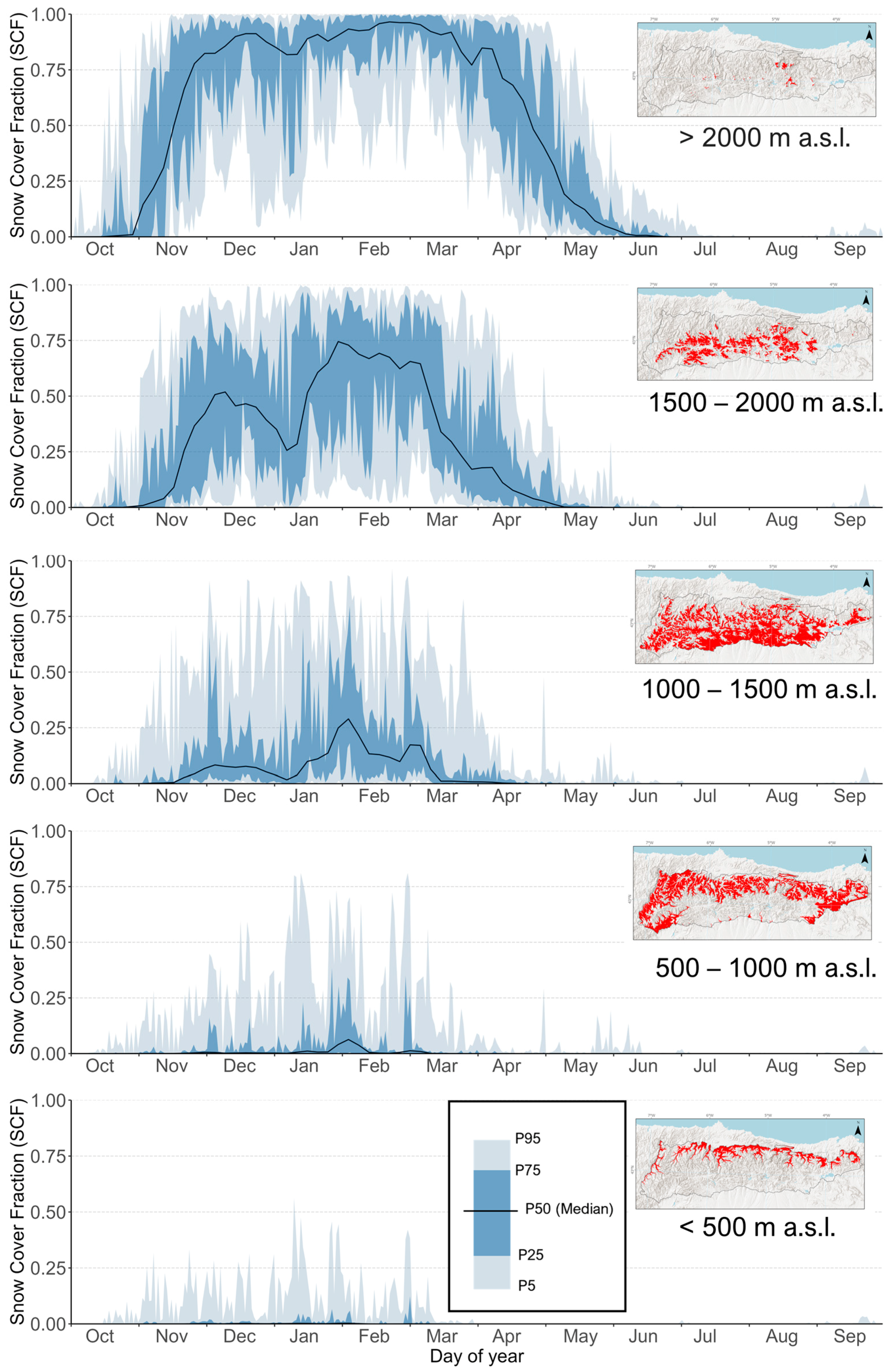
• Altitudinal Snow-Cover Fraction: the same calculation as SCF for 500 m altitudinal bands of the Cantabrian Mountains: SCF < 500 m; SCF 500–1000 m: SCF 1000–1500 m; SCF 1500–2000 m; SCF > 2000 m. The chosen model is the 1st coverage Digital Terrain Model (2009–2015) with a 25 m grid spacing (MDT25) from Spain’s National Cartographic System. It was created from LiDAR point clouds of the PNOA-LiDAR project (2009–2015), has a resolution of 25 m, and a vertical resolution of 0.001 m (https://www.idee.es/csw-inspire-idee/srv/spa/catalog.search?#/metadata/spaignMDT25, accessed on 31 July 2024).
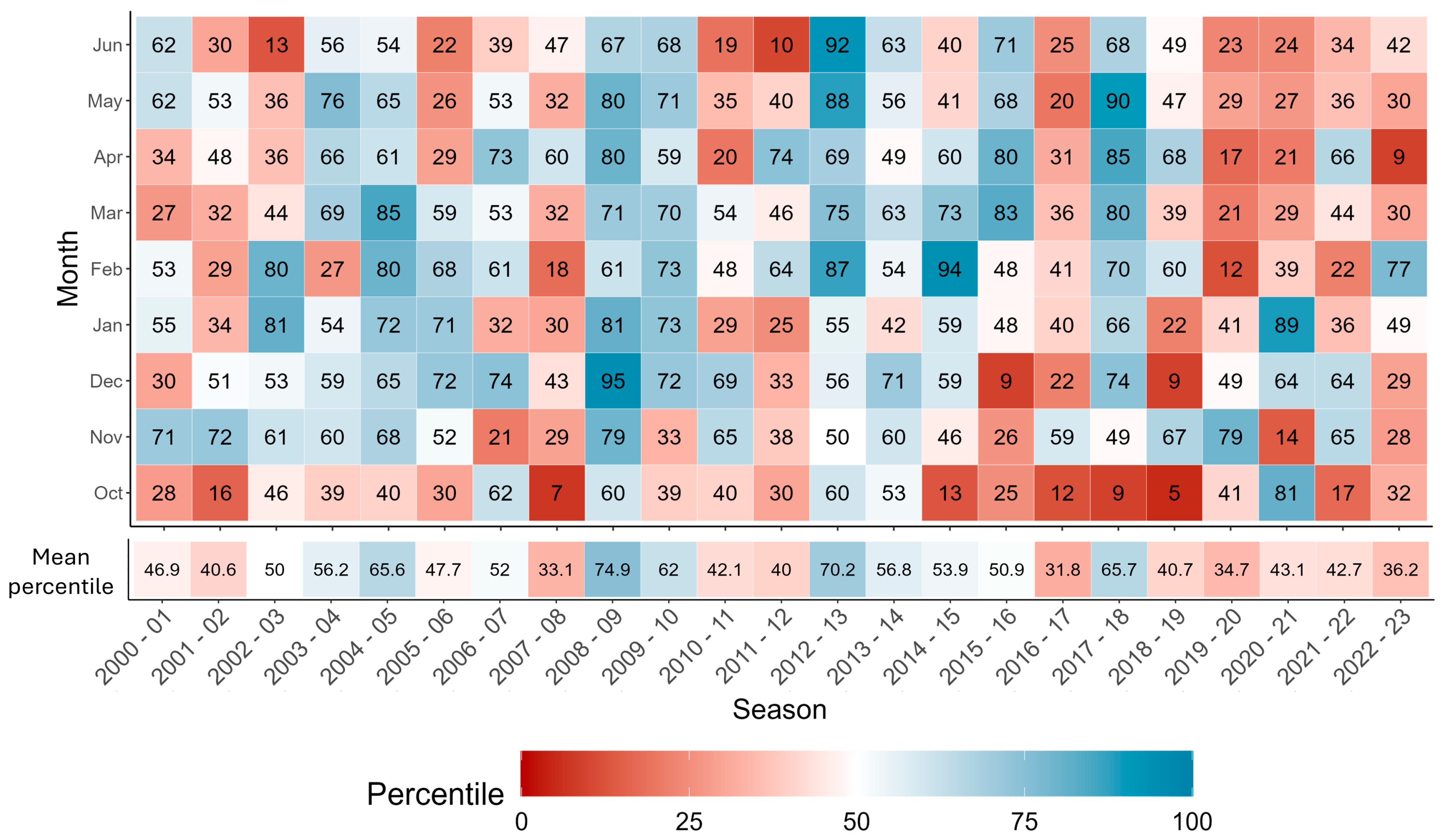
• Percentile of the average monthly SCF value. For each month of each year, the average SCF is calculated and compared to the monthly value for each season, once the data are ordered from lowest to highest. The percentile indicates the position of a value within a dataset, showing the value below which a given percentage of observations are found. For example, the 50th percentile represents the median value, where half of the observations are below and half are above. Values close to the 0th percentile are exceptionally low for that month, while values close to the 100th percentile are exceptionally high compared to the records for that month during the period 2000–2023. It has only been carried out for the months from October to June, because in July, August and September the snow cover is practically non-existent.

Although all the analysis was performed using Google Earth Engine, the cartographic representation of the final results was carried out using ArcGIS Pro 2.7.0 and is presented in the ArcGIS map viewers found in the Supplementary Materials.

3. Results

The monitoring of snow cover using satellite imagery can be developed at different scales. Pixel-level analysis of the occurrence of snow presence leads to the first section on Snow-Cover Days (SCDs) and the analysis of SCDs trends in the second section. After that, the extent of snow cover at the mountain range level is evaluated through the Snow-Cover Fraction in the third section.

3.1. Snow-Cover Days (SCDs)

The frequency of snow cover, and therefore the duration of snow cover, exhibits high variability in the Cantabrian Mountains (Figure 5), with a considerable altitudinal gradient. On average, the mean annual snow days in the Cantabrian Mountains (

Table 4. Main statistics of Snow-Cover Days (SCDs, in days) by altitude ranges in the Cantabrian Mountains.

	Mean SCDs (2000–2023)	Standard Deviation SCDs (2000–2023)	SCDs Maximum Mean Pixel (2000–2023)
Cantabrian Mountains (0–2650 m a.s.l.)	30.1	26.3	307.6
>2000 m a.s.l.	131.6	40.9	307.6
1500–2000 m a.s.l.	69.0	29.6	231.9
1000–1500 m a.s.l.	29.6	16.1	75.7
500–1000 m a.s.l.	15.5	7.9	39.7
<500 m a.s.l.	5.7	3.6	13.1

) is 30.1 days in the period 2000–2023, but with significant spatial variability explained by the relief of the mountain range. SCDs increase with altitude, averaging 5.7 days in the 0–500 m range, 15.5 days in the 500–1000 m range, 29.6 days in the 1000–1500 m range, 69 days in the 1500–2000 m range, and 131.6 days on average above 2000 m. In the higher-altitude sectors, Snow-Cover Days largely depends on local topography, with significant differences between slopes of the same massif. Thus, the highest SCD values are found in the depressions and shaded areas of the Picos de Europa National Park massifs (in these sectors, the average SCDs approaches 300 days) and on E–NE-facing slopes of the highest altitudes of the massifs, such as in the case of Peña Ubiña Massif and Fuentes Carrionas Massif (maximum SCDs of 200–250 days). A north–south asymmetry occurs because of the different altitudinal gradient of both slopes of the Cantabrian Mountains. Thus, the southern half of the Cantabrian Mountains has a higher average of SCD values.

3.2. Trends in Snow-Cover Days (SCDs)

The SCDs trend has been analysed and reflects a general decrease in SCDs, being more intense in some sectors of the Cantabrian Mountains. Thus, it is experiencing an average decrease of −0.26 days/year in Snow-Cover Days for the period 2000–2023 (

Table 5. Absolute, relative, and significant trend values (2000–2023) of Snow-Cover Days (SCDs) by altitudes in the Cantabrian Mountains.

	Absolute Trend (Days/Year)	Absolute Significant Trend Areas (Days/Year) (95% Confidence Level)	Relative Trend (%/Year)	Relative Significant Trend Areas (%/Year) (95% Confidence Level)
Cantabrian Mountains (0–2650 m a.s.l.)	−0.258	−0.921	−1.003	−2.459
>2000 m a.s.l.	−0.581	−1.395	−0.582	−1.470
1500–2000 m a.s.l.	−0.789	−1.350	−1.542	−2.497
1000–1500 m a.s.l.	−0.257	−0.906	−1.157	−3.153
500–1000 m a.s.l.	−0.089	−0.235	−0.890	−2.501
<500 m a.s.l.	−0.002	−0.015	−0.056	−0.353

). By altitudes, a higher absolute decline has been recorded in the higher altitudinal ranges, as while in the 0–500 m range the trend is negative but very close to zero, in the 500–1000 m range it is −0.08 days per year, and for 1000–1500 m it is −0.25 days per year. The largest declines occur in the 1500–2000 m range; with a loss of −0.78 days/year and in the range above 2000 m the decline is −0.58 days/year. Given the high variability of SCDs in the mountain range, it is worth observing the relative trend. The Cantabrian Mountains experience a −1% annual decline, reaching −1.5% annually in the 1500–2000 m range. Furthermore, considering only the areas with a significant trend at the 95% confidence interval, the trend is −0.92 days per year for the entire Cantabrian Mountains, which in relative terms equates to −2.45% annually. Spatially, the trend is uneven and more marked on the southern slope of the Cantabrian Mountains, especially in the western sectors (Sierra de Ancares, Sierra de Gistredo…). Some areas of the central sector of the Cantabrian Mountains experience slightly positive but not significant trends at its highest elevations (Figure 6).

3.3. Daily Extent of Snow Cover at Mountain Range Level: The Snow-Cover Fraction (SCF)

The calculation of the daily SCF makes possible checking the extent of snow cover throughout the mountain range, with higher values in the case of widespread snowfall events that have led to a high portion of the range covered by snow, or are indicative of a lower snowline, which equally causes an increase in the extent of snow cover in the whole or part of the range.

The daily aggregate of SCF from the 2000 to 2023 seasons (Figure 7) enables observing the annual behaviour of the snow cover. The values show high variability, with a daily mean SCF value of 0.074 and a standard deviation of 0.09. In general, the snow season usually begins in early November, with low SCF values, which usually cover only the highest altitudes, although they have also exceptionally occurred at the end of October in the analysed period. The mean SCF tends to increase significantly throughout November, remaining stable in December or slightly decreasing until the first half of January. After that, a considerable increase usually occurs, reaching the maximum SCF in late January-early February, with a value close to 0.25. In this case, high variability is also observed, with the highest percentiles being far from the median values. Thus, a period of progressive snowmelt occurs, with intermittent increases due to new snowfall episodes, highlighting the recurrence of snowfall event peaks in late February, which lead to a slight increase of SCF median and percentile 75 at that time. The largest decrease usually occurs throughout March, and finally, by the end of April, when the SCF approaches zero, with sporadic snowfall events being less common throughout May and early June, which can lead to low SCF values.

Figure 8 depicts the seasonal SCF dynamics across altitude ranges, emphasizing distinct seasonal patterns. Both the SCF value and the duration and stability of the snow cover increase with altitude. In the range of altitudes above 2000 m, the SCF increases rapidly throughout November (exceptionally in October), reaching stable values above 0.75 and close to 1 during the months of December to March, and then registering a progressive decrease extending into June, and exceptionally until July. In the 1500–2000 m range, the initial increase tends to occur slightly later, until December, here with a notable downward trend until mid-January (even reaching values close to zero in the first quartile). During January, a rapid growth to maximum values tends to occur, maintaining values between 0.5 and 0.75 until March. At this moment, a sharp decrease occurs until early May, and exceptionally, until early June. In the 1000–1500 m range, which occupies a larger extent of the Cantabrian Mountains (especially on the southern slope), the season usually begins in mid-November (exceptionally from late October), and maintains low median values until early January, when it begins to increase until reaching its maximum value in early February. It decreases irregularly until mid-March, when it tends to approach zero (exceptionally until late May). This range shows high interannual variability, with the 75th percentile values significantly higher than the median in early December and from mid-January to March, when it exceeds the SCF value of 0.5 and even approaches values of 0.75. In the 1000–500 m range, located on the northern slope and eastern and western extremes of the study area, the season tends to have a shorter duration, exceeding only 0.25 values exceptionally from late November to early March, and reaching values close to 0.75 exceptionally between January and February. In the range below 500 m (northernmost part of the study area), the presence of snow cover is rare (median close to zero throughout the season) and reaches its maximum value in January, with values close to 0.5 very exceptionally (95th percentile).

The analysis of 23 seasons has resulted in an uneven pattern in the SCF percentile, which can vary significantly from month to month in the case of a rapid melting or accumulation event of snow cover over a wide area. An irregular distribution of percentiles is observed (Figure 9), leading to seasons with SCF values above the median for almost the entire season, such as the 2004–2005 (P_mean = 65.6), 2008–2009 (P_mean = 74.9, season with the highest SCF), 2012–2013 (P_mean = 70.2), or 2017–2018 (P_mean = 65.7) seasons, and other seasons with values below the median for most of the season, such as 2001–2002 (P_mean = 40.6), 2007–2008 (P_mean = 33.1), 2016–2017 (P_mean = 31.8, season with the lowest SCF), 2019–2020 (P_mean = 34.7), 2022–2023 (P_mean = 36.2), and the rest of the seasons with parts of the season above and others below median values. A trend towards significantly lower percentiles is observed from the 2018–2019 season to the end of the study period. Some months stand out with exceptionally high SCF for the corresponding month (~P90): December 2008, June 2013, February 2015, May 2018, and January 2021 (0.89). Among the months with exceptionally low SCF (<P10) are October 2007, June 2012, December 2015, October 2017, October 2018, December 2018, and April 2023.

4. Discussion

4.1. Advantages and Limitations in the Detection of Snow Cover Using Satellite Imagery in Google Earth Engine

The use of Google Earth Engine facilitates the massive processing of satellite images to detect snow cover conditions in detail [38,39,40,46,48,49]. Processing large volumes of satellite images in the cloud significantly reduces computational costs [37], which is mandatory considering that more than 10,800 satellite images have been used for this study.

Tools such as SnowWarp [45], developed in Google Earth Engine, are considered a relevant precedent in the methodology applied in this article. The difference with that tool lies in the fact that for this study, more than 4000 Sentinel-2 images were used for the analyses related to SCDs. Furthermore, this work analyses trends in the frequency of snow cover and conducts an analysis of anomalies relative to normal monthly values.

The integration of multiple satellite platforms for the creation of a daily snow cover collection of images enhances both the spatial and temporal resolution of observations [49,64,68,73,74]. Moreover, in the case of Sentinel and Landsat images, whose swath width does not cover the entirety of the Cantabrian Mountains due to their longitudinal arrangement, their combination with MODIS pixels serves as an excellent complement to achieve full daily coverage of the study area. It is important to consider that the records from the three satellites are simultaneous. Hence, during the period 2000–2015, records are made solely with MODIS and Landsat images, and then Sentinel-2 is incorporated, offering higher spatial resolution. Introducing Sentinel-2 pixels into trend analyses would be problematic in some cases because it would significantly alter the frequencies of snow cover in 500 m MODIS pixels when a pixel with complex topography has high variability.

The detection of snow cover through satellite imagery, while highly beneficial for monitoring large and remote areas [63,75], comes with several limitations. One of the primary challenges is cloud cover, which can hide the study area surface either partially or entirely, creating data gaps [46]. This is especially problematic in regions where cloud cover is persistent and frequent. For instance, in the Cantabrian Mountains, cloud-cover distribution is heterogeneous (Figure 4b), causing greater uncertainty in some areas of the northern slope. This area has been classified as medium to high suitability for Sentinel data due to its high coverage of satellite passes and moderate cloudiness [32]. Additionally, the time elapsed between snowfall events and snow melt can sometimes be a few hours or days, especially in the lower altitudes of the mountain range, where snow dynamics are very changeable. This may result in some ephemeral snow cover going undetected in cases where clouds persist throughout the snowfall and subsequent melting episode. There is also an underestimation issue in areas with dense forest cover when detecting snow via satellite [33,34], as snow can remain on the ground under the tree canopies and not on the top of the canopies, making it undetectable by the passive sensors used in this study.

Regarding the classification of images to determine daily snow cover, an NDSI threshold of values greater than 0.4 is commonly accepted for the binary categorization of snow-covered and non-covered areas [76], especially when the spatial resolution is below 500 m. However, adjustments may be required in areas with complex topography or depending on vegetation or image illumination. In this study, the daily snow-cover classification has been visually evaluated using raw satellite images, as well as other snow classification products like the Theia Snow collection [77], achieving correlations of over R² > 0.8 in the analysed cases, which included the yearly Snow Data products (Level 3) for the 2018, 2019, 2020, and 2021 seasons, and some single-temporal images (Level 2), available at https://www.theia-land.fr/en/product/snow (accessed on 31 July 2024).

The classification of snow cover, which could sometimes be confused with bodies of water, has been resolved through the manual masking of reservoirs, supported by the NDWI (Normalized Difference Water Index). The Cantabrian Mountains do not face the issue of distinguishing between snow/ice-covered areas due to the absence of active glaciers (only small ice patches exist in the Picos de Europa National Park), as is the case in other higher-altitude or higher-latitude mountain ranges.

The high spatial and interannual variability of snow cover in the Cantabrian Mountains would make necessary the analysis of longer satellite image series in future studies, as 23 years may be insufficient for detecting significant trends in the most variable areas.

4.2. Comparison of SCD Values Obtained in Other Studies

The results obtained on SCDs (Figure 5), which measure the duration of snow cover based on the frequency of snow-cover occurrence through satellite images, offer comparable and consistent data in relation to other studies, such as in Alonso-González et al. [78]. This study showed probabilities of snow-cover occurrence in the period 1980–2014 of 4.3% for the 1000 m elevation band; 19% for the 1500 m range, and 37% above 2000 m (8%; 18.9%; 36% respectively obtained in this study for the period 2000–2023). The Cantabrian Mountains are the mountain range in the Iberian Peninsula with the second-highest values of snow-cover frequency and variability, behind the Pyrenees. The 1500–2000 m range of the Cantabrian Mountains shows the highest duration values of all mountains in the Iberian Peninsula (only in that altitudinal range) [78].

Other studies have quantified the SCDs in the Cantabrian Mountains, but at a more local scale. In Picos de Europa, the duration of snow cover has also been quantified at 8 to 9 months above 2000 m and 6 months above 1500 m [51], which matches with satellite records showing areas favourable for snow accumulation and longer snow-cover duration, with values above 240 days, reaching average values over 300 days in areas of maximum accumulation. Records analysed by Ruiz-Fernández et al. [62] quantified SCD values exceeding 11 months in permanent snowfields in the central and western massifs of Picos de Europa. In the Hoyo Empedrado glacial cirque, located in the Fuentes Carrionas Massif, estimations between 2006 and 2020 based on ground temperature records also indicated average SCD values between 126 and 266 days, with significant spatial variability influenced by local topography [79]. These values are close to, though slightly higher than, those recorded by satellite for the period 2000–2023, which ranged between 120 and 200 days. Between 2002 and 2009, snow patches in the western sector of the Cantabrian Mountains, such as Joyas del Nevadín and Valdeiglesia, were estimated to have a SCD value of 237 days and 220 days, respectively [80], values notably higher than the average satellite records shown for the period 2000–2023, although it is one of the areas showing a significant decreasing trend. The study by Gallinar-Cañedo et al. [58] showed isotherm temperature records of 6 to 8 months above 1800 m in the Peña Ubiña Massif, which coincides with the satellite SCD records, reaching an average SCDs of more than 200 days in the period 2000–2023, according to the results. It also shows the interannual variability of snow-cover duration in the analysed period 2012–2018, greatly influenced by the unstable duration of superficial snow patches.

It is important to note that the study of permanent snow patches requires detailed analysis with higher resolution satellites, such as Sentinel-2, as the SCD records at a very local scale in areas with high variability within a single MODIS pixel (500 m) may mask an overestimation of SCDs in rugged areas where snow lasts for a shorter period, and an underestimation in areas where local topography controls snow cover, which occurs especially during the final phase of the snow season [68].

4.3. Trends in Snow-Cover Duration in Nearby Mountain Ranges

Satellite records have allowed the quantification of the regressive trend of snow cover of −0.44 days/year globally since the year 2000 [81]. In mountainous areas, 78% of mountain ranges show decreasing trends in snow-cover duration [82]. In the Northern Hemisphere, the shortening of snow-cover duration is more intense in high-altitude and high-latitude areas, where some perennial snow covers are turning seasonal [83]. This decline is generally attributed to a reduction in snow cover in spring [84]. In Eurasia, an earlier snowmelt is associated with higher-than-average temperatures during the months of snowmelt [85].

In the Cantabrian Mountains, the analysis has quantified the observed trends in snow cover (Table 5), showing declines for the entire range of −0.26 days per year (−1% annually), and −0.92 days per year (−2.46% annually) for areas with a 95% significant trend. In mountainous regions of western Europe, a decline in snow cover has also been observed in recent decades [86,87] and in the Moroccan Atlas [88], although with high spatial variability. For example, in the Alps, the trend is not significant for the entire range, but it is in some areas [89]; in the Pyrenees, declining trends of snow-cover duration and average snow accumulation were only significant in the 2100 m altitude range [90] and were more pronounced in the western area. This declining snow-cover trend has been observed since the mid-1980s in the Alto Sil, located in the western sector of the Cantabrian Mountains [80].

The high intra-annual and spatial variability of the snow season duration may be driven by a delayed snow onset day, an earlier snow disappearance date, or both. A detailed study of these factors is planned for future work in the Cantabrian Mountains, with greater detail, to accurately quantify these changes.

4.4. Seasonal Regime of SCF in the Cantabrian Mountains: Comparison with Nearby Areas and Climate Reanalysis Products

Regarding SCF, the observation of a highly irregular interannual SCF distribution (Figure 7) is favoured by the succession of snowfall events throughout the season at different times of the year. Snowfall events can be intense and promote a rapid change in the general conditions of the snow cover, which in the Cantabrian Mountains can quickly shift from minimum to maximum annual distribution values. The records show a seasonal regime with a distribution like that observed in other nearby mountain ranges. For example, the study by Marchane et al. [88] also shows in the Atlas Mountains (although at higher altitudes) a progressive increase in the snow-covered area from November to the peak at the end of January–early February, but with a decrease between December and January. This common pattern, very marked in the Cantabrian Mountains in the 1500–2000 m range (Figure 8), may be related to different teleconnection patterns, being the NAO index one of the most important teleconnections that influences winter precipitation (DJFM) in the western Iberian Peninsula, following a study for the period 1948–2008 in León, in the south of the Cantabrian Mountains [91]. Additionally, they report a negative trend in winter precipitation and an increase in anticyclonic weather types during the winter months, especially since the 1980s. It has been demonstrated that the NAO index has a moderate negative correlation with snow-cover duration from December to March, ranging from 0.3 to 0.6, being higher on the southern slope of the Cantabrian Mountains and increasing towards the west [92,93]. This could explain the decline in snow cover during the second half and first part of January, as an increase trend in positive NAO phases during winter months is reported is the area, resulting in a lower number of snowfall events [59].

The SCF records have been compared with the ‘snow_cover’ variable data from the ERA5-Land climate reanalysis product [72]. It is important to consider the different spatial resolutions of both products: while the SCF calculated using satellite imagery has a resolution of up to 20 m, ERA5-Land is produced with a resolution of 0.1° (11,132 m). The SCF records with ERA5-Land (Figure 10a) show a very similar pattern for the entire Cantabrian Mountain Range compared to the satellite records. A slight underestimation of snow cover is observed with ERA5-Land, except during the peak snow accumulation period around February, where it slightly overestimates. They also show a high correlation in daily SCF values (Figure 10b), with a correlation of 0.92 for the period 2000–2023.

5. Conclusions

• Monitoring snow cover through satellite images enables continuous tracking of snow conditions, regardless of the availability of ground-based observations. Google Earth Engine has facilitated the processing of 10,831 satellite images from Sentinel-2, Landsat 5, Landsat 8, and Terra-MODIS to identify snow cover.
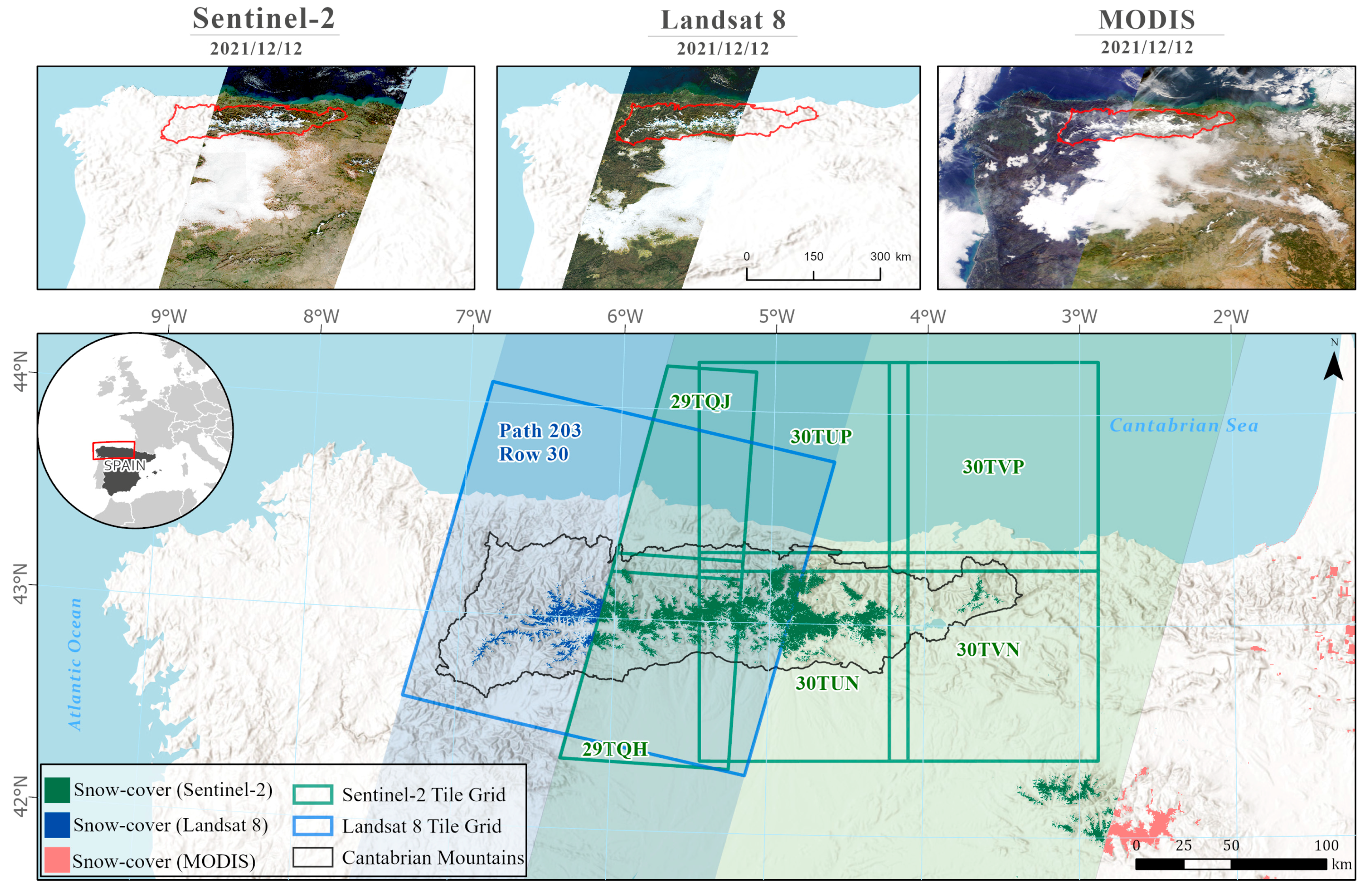
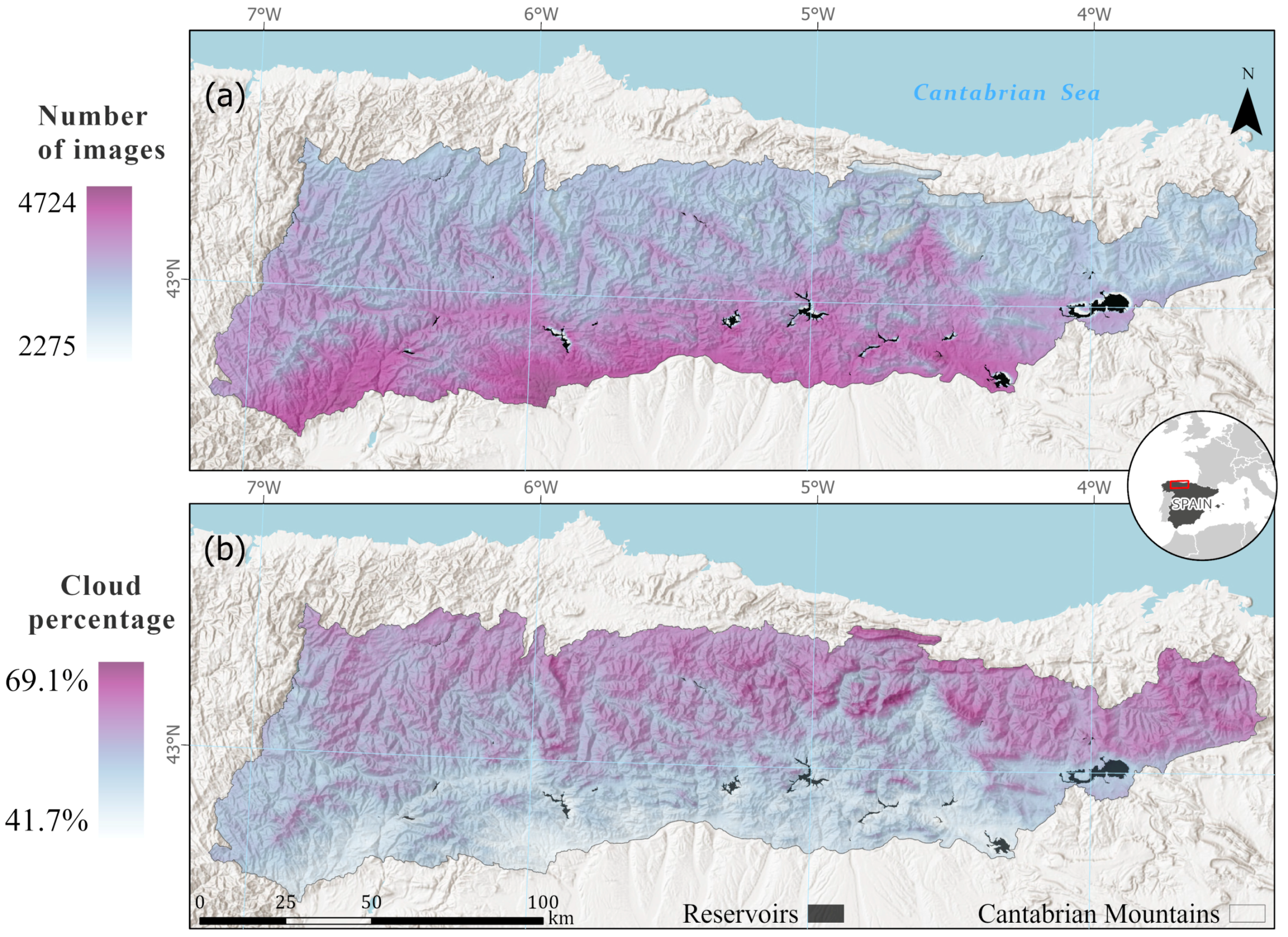
• Detecting snow cover presents challenges in areas such as steep slopes and forested regions and during prolonged cloud cover, often leading to underestimation of snow cover in these zones. Cloud cover (which ranged from 41.7% to 69.1%) was masked out in the analysis. Integrating multiple satellite data sources reduces data gaps and improves coverage. The hierarchical pixel method using data from three satellites achieves optimal spatial resolution when feasible. Additionally, temporal gap-filling techniques address data absences caused by cloud cover, which could last up to 5 days. The combination of Sentinel and Landsat data, despite their limited swath width, with MODIS pixels provides comprehensive coverage of the entire study area.
• The Cantabrian Mountains exhibit a very irregular distribution of snow-cover days, highly influenced by altitude and local topography. The average duration of snow cover in the Cantabrian Mountains is 30.1 days, with significant differences across altitudinal zones, ranging from 5.7 days below 500 m to an average of 131.6 days above 2000 m, with durations exceeding 300 days in reduced elevated areas, where snow accumulation and topography favour its persistence for nearly the entire year.
• Decreasing trends in the duration of snow cover have been observed in most parts of the Cantabrian Mountains, more intensely on the southern slope, with hardly any longitudinal gradient. The overall trend in duration for the period 2000–2023 is −0.26 days/year, with the most significant decrease observed in the 1500–2000 m range (−0.78 days/year), implying annual losses of around 1–1.5%. In areas with significant trends, mainly located in the southwestern and southeastern massifs of the Cantabrian Mountains, the decline is pronounced, at −0.9 days/year and −1.3 days/year in areas above 1500 m, representing an annual decrease of around 1.5–3.1% in areas with significant trend.
• The analysis of SCF has revealed differences in the duration of snow cover, which has an irregular pattern throughout the season. Differences across altitudinal zones were analysed on a seasonal scale, observing more stable snow cover patterns at higher altitudinal zones (>2000 m), but with significant interannual variations in all altitudinal ranges.
• The aggregation of SCF by percentiles on a monthly scale has allowed the detection of seasons with greater snow cover (such as 2008–2009) compared to seasons with anomalously low snow cover (2016–2017), as well as identifying specific months where snow cover is exceptionally high (such as February 2015, ranked in the 94th percentile of conditions recorded in February) or low (such as October or December 2018, with a percentile below 10).
• The methodology employed in this article using satellite images is a very useful tool, especially for areas with sparse snow observation networks. This methodology, which has enabled the extraction of a daily time series of snow cover for the Cantabrian Mountains, could be analysed on a more local scale in future works, or even supported by other forms of on-ground snow observation, such as webcam images.

References

1. Qin, Y.; Abatzoglou, J.T.; Siebert, S.; Huning, L.S.; AghaKouchak, A.; Mankin, J.S.; Hong, C.; Tong, D.; Davis, S.J.; Mueller, N.D. Agricultural Risks from Changing Snowmelt. Nat. Clim. Chang. 2020, 10, 459–465. [Google Scholar] [CrossRef]
2. Mankin, J.S.; Viviroli, D.; Singh, D.; Hoekstra, A.Y.; Diffenbaugh, N.S. The Potential for Snow to Supply Human Water Demand in the Present and Future. Environ. Res. Lett. 2015, 10, 114016. [Google Scholar] [CrossRef]
3. García-Ruiz, J.M.; Arnáez, J.; Lasanta, T.; Nadal-Romero, E.; López-Moreno, J.I. Snow in the Mountains. In Mountain Environments: Changes and Impacts. Natural Landscapes and Human Adaptations to Diversity; Negm, A.M., Chaplina, T., Eds.; Springer: Cham, Switzerland, 2024; pp. 117–137. [Google Scholar] [CrossRef]
4. Vajda, A.; Tuomenvirta, H.; Juga, I.; Nurmi, P.; Jokinen, P.; Rauhala, J. Severe Weather Affecting European Transport Systems: The Identification, Classification and Frequencies of Events. Nat. Hazards 2014, 72, 169–188. [Google Scholar] [CrossRef]
5. Haeberli, W.; Whiteman, C. Snow and Ice-Related Hazards, Risks, and Disasters: A General Framework. In Snow Ice-Relat. Hazards Risks Disasters; Shroder, J.F., Haeberli, W., Whiteman, C., Eds.; Elsevier: Amsterdam, The Netherlands, 2015; pp. 1–34. [Google Scholar] [CrossRef]
6. Schweizer, J.; Jamieson, J.B.; Schneebeli, M. Snow Avalanche Formation. Rev. Geophys. 2003, 41, 1016. [Google Scholar] [CrossRef]
7. Eckerstorfer, M.; Bühler, Y.; Frauenfelder, R.; Malnes, E. Remote Sensing of Snow Avalanches: Recent Advances, Potential, and Limitations. Cold Reg. Sci. Technol. 2016, 121, 126–140. [Google Scholar] [CrossRef]
8. Fayad, A.; Gascoin, S.; Faour, G.; López-Moreno, J.I.; Drapeau, L.; Le Page, M.; Escadafal, R. Snow Hydrology in Mediterranean Mountain Regions: A Review. J. Hydrol. 2017, 551, 374–396. [Google Scholar] [CrossRef]
9. Tramblay, Y.; Koutroulis, A.; Samaniego, L.; Vicente-Serrano, S.M.; Volaire, F.; Boone, A.; Le Page, M.; Llasat, M.C.; Albergel, C.; Burak, S.; et al. Challenges for Drought Assessment in the Mediterranean Region under Future Climate Scenarios. Earth Sci. Rev. 2020, 210, 103348. [Google Scholar] [CrossRef]
10. Beniston, M.; Stoffel, M. Rain-on-Snow Events, Floods and Climate Change in the Alps: Events May Increase with Warming up to 4 °C and Decrease Thereafter. Sci. Total Environ. 2016, 571, 228–236. [Google Scholar] [CrossRef]
11. Morán-Tejeda, E.; López-Moreno, J.I.; Stoffel, M.; Beniston, M. Rain-on-Snow Events in Switzerland: Recent Observations and Projections for the 21st Century. Clim. Res. 2016, 71, 111–125. [Google Scholar] [CrossRef]
12. Morán-Tejeda, E.; Fassnacht, S.R.; Lorenzo-Lacruz, J.; López-Moreno, J.I.; García, C.; Alonso-González, E.; Collados-Lara, A.J. Hydro-Meteorological Characterization of Major Floods in Spanish Mountain Rivers. Water 2019, 11, 2641. [Google Scholar] [CrossRef]
13. Corripio, J.G.; López-Moreno, J.I. Analysis and Predictability of the Hydrological Response of Mountain Catchments to Heavy Rain on Snow Events: A Case Study in the Spanish Pyrenees. Hydrology 2017, 4, 20. [Google Scholar] [CrossRef]
14. Di Mauro, B.; Fava, F.; Ferrero, L.; Garzonio, R.; Baccolo, G.; Delmonte, B.; Colombo, R. Mineral Dust Impact on Snow Radiative Properties in the European Alps Combining Ground, UAV, and Satellite Observations. J. Geophys. Res. Atmos. 2015, 120, 6080–6097. [Google Scholar] [CrossRef]
15. Réveillet, M.; Dumont, M.; Gascoin, S.; Lafaysse, M.; Nabat, P.; Ribes, A.; Nheili, R.; Tuzet, F.; Ménégoz, M.; Morin, S.; et al. Black Carbon and Dust Alter the Response of Mountain Snow Cover under Climate Change. Nat. Commun. 2022, 13, 5279. [Google Scholar] [CrossRef]
16. Dumont, M.; Tuzet, F.; Gascoin, S.; Picard, G.; Kutuzov, S.; Lafaysse, M.; Cluzet, B.; Nheili, R.; Painter, T.H. Accelerated Snow Melt in the Russian Caucasus Mountains after the Saharan Dust Outbreak in March 2018. J. Geophys. Res. Earth Surf. 2020, 125, e2020JF005641. [Google Scholar] [CrossRef]
17. García-Ruiz, J.M.; López-Moreno, I.I.; Vicente-Serrano, S.M.; Lasanta-Martínez, T.; Beguería, S. Mediterranean Water Resources in a Global Change Scenario. Earth Sci. Rev. 2011, 105, 121–139. [Google Scholar] [CrossRef]
18. Morán-Tejeda, E.; Ceballos-Barbancho, A.; Llorente-Pinto, J.M. Hydrological Response of Mediterranean Headwaters to Climate Oscillations and Land-Cover Changes: The Mountains of Duero River Basin (Central Spain). Glob. Planet. Chang. 2010, 72, 39–49. [Google Scholar] [CrossRef]
19. López-Moreno, J.I.; Gascoin, S.; Herrero, J.; Sproles, E.A.; Pons, M.; Alonso-González, E.; Hanich, L.; Boudhar, A.; Musselman, K.N.; Molotch, N.P.; et al. Different Sensitivities of Snowpacks to Warming in Mediterranean Climate Mountain Areas. Environ. Res. Lett. 2017, 12, 074006. [Google Scholar] [CrossRef]
20. Sanmiguel-Vallelado, A.; Morán-Tejeda, E.; Alonso-González, E.; López-Moreno, J.I. Effect of Snow on Mountain River Regimes: An Example from the Pyrenees. Front. Earth Sci. 2017, 11, 515–530. [Google Scholar] [CrossRef]
21. Thornton, J.M.; Palazzi, E.; Pepin, N.C.; Cristofanelli, P.; Essery, R.; Kotlarski, S.; Giuliani, G.; Guigoz, Y.; Kulonen, A.; Pritchard, D.; et al. Toward a Definition of Essential Mountain Climate Variables. One Earth 2021, 4, 805–827. [Google Scholar] [CrossRef]
22. The 2022 GCOS Implementation Plan (GCOS-244). Available online: https://library.wmo.int/records/item/58104-the-2022-gcos-implementation-plan-gcos-244 (accessed on 23 July 2024).
23. Schaffhauser, A.; Adams, M.; Fromm, R.; Jörg, P.; Luzi, G.; Noferini, L.; Sailer, R. Remote Sensing Based Retrieval of Snow Cover Properties. Cold Reg. Sci. Technol. 2008, 54, 164–175. [Google Scholar] [CrossRef]
24. Nolin, A.W. Recent Advances in Remote Sensing of Seasonal Snow. J. Glaciol. 2010, 56, 1141–1150. [Google Scholar] [CrossRef]
25. Dietz, A.J.; Kuenzer, C.; Gessner, U.; Dech, S. Remote Sensing of Snow—A Review of Available Methods. Int. J. Remote Sens. 2012, 33, 4094–4134. [Google Scholar] [CrossRef]
26. Matiu, M.; Jacob, A.; Notarnicola, C. Daily MODIS Snow Cover Maps for the European Alps from 2002 Onwards at 250 m Horizontal Resolution along with a Nearly Cloud-Free Version. Data 2019, 5, 1. [Google Scholar] [CrossRef]
27. Dedieu, J.P.; Lessard-Fontaine, A.; Ravazzani, G.; Cremonese, E.; Shalpykova, G.; Beniston, M. Shifting Mountain Snow Patterns in a Changing Climate from Remote Sensing Retrieval. Sci. Total Environ. 2014, 493, 1267–1279. [Google Scholar] [CrossRef] [PubMed]
28. Salzano, R.; Salvatori, R.; Valt, M.; Giuliani, G.; Chatenoux, B.; Ioppi, L. Automated Classification of Terrestrial Images: The Contribution to the Remote Sensing of Snow Cover. Geosciences 2019, 9, 97. [Google Scholar] [CrossRef]
29. Dozier, J. Spectral Signature of Alpine Snow Cover from the Landsat Thematic Mapper. Remote Sens. Environ. 1989, 28, 9–22. [Google Scholar] [CrossRef]
30. Hall, D.K.; Riggs, G.A.; Salomonson, V.V. Development of Methods for Mapping Global Snow Cover Using Moderate Resolution Imaging Spectroradiometer Data. Remote Sens. Environ. 1995, 54, 127–140. [Google Scholar] [CrossRef]
31. Hall, D.K.; Riggs, G.A. Normalized-Difference Snow Index (NDSI). In Encyclopedia of Earth Sciences Series; Springer: Dordrecht, The Netherlands, 2011; Part 3; pp. 779–780. [Google Scholar] [CrossRef]
32. Sudmanns, M.; Tiede, D.; Augustin, H.; Lang, S. Assessing Global Sentinel-2 Coverage Dynamics and Data Availability for Operational Earth Observation (EO) Applications Using the EO-Compass. Int. J. Digit. Earth 2020, 13, 768–784. [Google Scholar] [CrossRef]
33. Gascoin, S.; Luojus, K.; Nagler, T.; Lievens, H.; Masiokas, M.; Jonas, T.; Zheng, Z.; De Rosnay, P. Remote Sensing of Mountain Snow from Space: Status and Recommendations. Front. Earth Sci. 2024, 12, 1381323. [Google Scholar] [CrossRef]
34. Muhuri, A.; Gascoin, S.; Menzel, L.; Kostadinov, T.S.; Harpold, A.A.; Sanmiguel-Vallelado, A.; Lopez-Moreno, J.I. Performance Assessment of Optical Satellite-Based Operational Snow Cover Monitoring Algorithms in Forested Landscapes. IEEE J. Sel. Top. Appl. Earth Obs. Remote Sens. 2021, 14, 7159–7178. [Google Scholar] [CrossRef]
35. Premier, V.; Marin, C.; Bertoldi, G.; Barella, R.; Notarnicola, C.; Bruzzone, L. Exploring the Use of Multi-Source High-Resolution Satellite Data for Snow Water Equivalent Reconstruction over Mountainous Catchments. Cryosphere 2023, 17, 2387–2407. [Google Scholar] [CrossRef]
36. Luo, J.; Dong, C.; Lin, K.; Chen, X.; Zhao, L.; Menzel, L. Mapping Snow Cover in Forests Using Optical Remote Sensing, Machine Learning and Time-Lapse Photography. Remote Sens. Environ. 2022, 275, 113017. [Google Scholar] [CrossRef]
37. Gorelick, N.; Hancher, M.; Dixon, M.; Ilyushchenko, S.; Thau, D.; Moore, R. Google Earth Engine: Planetary-Scale Geospatial Analysis for Everyone. Remote Sens. Environ. 2017, 202, 18–27. [Google Scholar] [CrossRef]
38. Velastegui-Montoya, A.; Montalván-Burbano, N.; Carrión-Mero, P.; Rivera-Torres, H.; Sadeck, L.; Adami, M. Google Earth Engine: A Global Analysis and Future Trends. Remote Sens. 2023, 15, 3675. [Google Scholar] [CrossRef]
39. Mutanga, O.; Kumar, L. Google Earth Engine Applications. Remote Sens. 2019, 11, 591. [Google Scholar] [CrossRef]
40. Zhao, Q.; Yu, L.; Li, X.; Peng, D.; Zhang, Y.; Gong, P. Progress and Trends in the Application of Google Earth and Google Earth Engine. Remote Sens. 2021, 13, 3778. [Google Scholar] [CrossRef]
41. Li, Z.; Liu, C.; Zhang, P.; Tian, B. Assessment of Snow Cover Product Using Google Earth Engine Cloud Computing Platform. Int. Geosci. Remote Sens. Symp. (IGARSS) 2018, 2018, 5203–5205. [Google Scholar] [CrossRef]
42. Torabi Poodeh, H.; Yousefi, H.; Samadi, A.; Arshia, A.; Shamsi, Z.; Yarahmadi, Y. Evaluation of Snow Cover Changes Trend Using GEE and TFPW-MK Test (Case Study: Marber Basin-Isfahan). Iran. J. Ecohydrol. 2021, 8, 195–204. [Google Scholar] [CrossRef]
43. Abdelkader, M.; Bravo Mendez, J.H.; Temimi, M.; Brown, D.R.N.; Spellman, K.V.; Arp, C.D.; Bondurant, A.; Kohl, H. A Google Earth Engine Platform to Integrate Multi-Satellite and Citizen Science Data for the Monitoring of River Ice Dynamics. Remote Sens. 2024, 16, 1368. [Google Scholar] [CrossRef]
44. Calizaya, E.; Laqui, W.; Sardón, S.; Calizaya, F.; Cuentas, O.; Cahuana, J.; Mindani, C.; Huacani, W. Snow Cover Temporal Dynamic Using MODIS Product, and Its Relationship with Precipitation and Temperature in the Tropical Andean Glaciers in the Alto Santa Sub-Basin (Peru). Sustainability 2023, 15, 7610. [Google Scholar] [CrossRef]
45. Laurin, G.V.; Francini, S.; Penna, D.; Zuecco, G.; Chirici, G.; Berman, E.; Coops, N.C.; Castelli, G.; Bresci, E.; Preti, F.; et al. SnowWarp: An Open Science and Open Data Tool for Daily Monitoring of Snow Dynamics. Environ. Model. Softw. 2022, 156, 105477. [Google Scholar] [CrossRef]
46. Gascoin, S.; Monteiro, D.; Morin, S. Reanalysis-Based Contextualization of Real-Time Snow Cover Monitoring from Space. Environ. Res. Lett. 2022, 17, 114044. [Google Scholar] [CrossRef]
47. Crumley, R.L.; Palomaki, R.T.; Nolin, A.W.; Sproles, E.A.; Mar, E.J. SnowCloudMetrics: Snow Information for Everyone. Remote Sens. 2020, 12, 3341. [Google Scholar] [CrossRef]
48. Sproles, E.A.; Crumley, R.L.; Nolin, A.W.; Mar, E.; Moreno, J.I.L. SnowCloudHydro—A New Framework for Forecasting Streamflow in Snowy, Data-Scarce Regions. Remote Sens. 2018, 10, 1276. [Google Scholar] [CrossRef]
49. El jabiri, Y.; Boudhar, A.; Htitiou, A.; Sproles, E.A.; Bousbaa, M.; Bouamri, H.; Chehbouni, A. A Method for Robust Estimation of Snow Seasonality Metrics from Landsat and Sentinel-2 Time Series Data over Atlas Mountains Scale Using Google Earth Engine. Geocarto Int. 2024, 39, 2313001. [Google Scholar] [CrossRef]
50. Ortega Villazán, M.T.; Morales Rodríguez, C.G. El Clima de La Cordillera Cantábrica Castellano-Leonesa: Diversidad, Contrastes y Cambios. Investig. Geogr. 2015, 63, 45–67. [Google Scholar] [CrossRef]
51. González Trueba, J.J.; Serrano Cañadas, E. Snow in the Picos de Europa: Geomorphological and Environmental Implications. Cuad. De Investig. Geogr. 2010, 36, 61–84. [Google Scholar] [CrossRef]
52. García-Hernández, C.; López-Moreno, J.I. Extreme Snowfalls and Atmospheric Circulation Patterns in the Cantabrian Mountains (NW Spain). Cold Reg. Sci. Technol. 2024, 221, 104170. [Google Scholar] [CrossRef]
53. Serrano Cañadas, E.; Gómez Lende, M.; Pisabarro Pérez, A.; Serrano Cañadas, E.; Gómez Lende, M.; Pisabarro Pérez, A. Nieve y Riesgo de Aludes En La Montaña Cantábrica: El Alud de Cardaño de Arriba, Alto Carrión (Palencia). Polígonos Rev. De Geogr. 2016, 28, 239–264. [Google Scholar] [CrossRef]
54. Beato Bergua, S.; Poblete Piedrabuena, M.Á.; Marino Alfonso, J.L. Snow Avalanches, Land Use Changes, and Atmospheric Warming in Landscape Dynamics of the Atlantic Mid-Mountains (Cantabrian Range, NW Spain). Appl. Geogr. 2019, 107, 38–50. [Google Scholar] [CrossRef]
55. Santos González, J.; Redondo Vega, J.M.; Gómez Villar, A.; González Gutiérrez, R.B. Avalanches in the Alto Sil (Western Cantabrian Mountain, Spain). Cuad. De Investig. Geogr. 2010, 36, 7–26. [Google Scholar] [CrossRef]
56. Del Valle Granda, E.; Bergua, S.B.; Pérez, C.R.; Arenas, D.H. Snow Avalanches Susceptibility on the Somiedo Road (Asturias) and Its Dissemination through Augmented Reality. Cuad. Geogr. 2024, 63, 297–317. [Google Scholar] [CrossRef]
57. García-Hernández, C.; Ruiz-Fernández, J.; Sánchez-Posada, C.; Pereira, S.; Oliva, M.; Vieira, G. Reforestation and Land Use Change as Drivers for a Decrease of Avalanche Damage in Mid-Latitude Mountains (NW Spain). Glob. Planet. Chang. 2017, 153, 35–50. [Google Scholar] [CrossRef]
58. Cañedo, D.G.; Ruiz-Fernández, J.; García-Hernández, C. La Nieve En El Macizo de Las Ubiñas (Montañas Cantábricas) y Sus Implicaciones Geomorfológicas. Boletín De La Asoc. De Geógr. Españoles 2022, 93, 4. [Google Scholar] [CrossRef]
59. Merino, A.; Fernández, S.; Hermida, L.; López, L.; Sánchez, J.L.; García-Ortega, E.; Gascón, E. Snowfall in the Northwest Iberian Peninsula: Synoptic Circulation Patterns and Their Influence on Snow Day Trends. Sci. World J. 2014, 2014, 480275. [Google Scholar] [CrossRef] [PubMed]
60. Pisabarro, A.; Pisabarro, A. Snow Cover as a Morphogenic Agent Determining Ground Climate, Landforms and Runoff in the Valdecebollas Massif, Cantabrian Mountains. Cuad. De Investig. Geogr. 2020, 46, 81–102. [Google Scholar] [CrossRef]
61. Pisabarro, A.; Pellitero, R.; Serrano, E.; Gómez-Lende, M.; González-Trueba, J.J. Ground Temperatures, Landforms and Processes in an Atlantic Mountain. Cantabrian Mountains (Northern Spain). CATENA 2017, 149, 623–636. [Google Scholar] [CrossRef]
62. Ruiz-Fernández, J.; García-Hernández, C.; Ochoa-Álvarez, M.; Van den Bergh, M.; Gallinar Cañedo, D.; González-Díaz, B. Ground and Near-Rock Surface Air Thermal Regimes in the High Mountain of the Picos de Europa (Cantabrian Mountains, NW Spain). Air Soil. Water Res. 2023, 16, 11786221231176676. [Google Scholar] [CrossRef]
63. Alonso-González, E.; Gutmann, E.; Aalstad, K.; Fayad, A.; Bouchet, M.; Gascoin, S. Snowpack Dynamics in the Lebanese Mountains from Quasi-Dynamically Downscaled ERA5 Reanalysis Updated by Assimilating Remotely Sensed Fractional Snow-Covered Area. Hydrol. Earth Syst. Sci. 2021, 25, 4455–4471. [Google Scholar] [CrossRef]
64. Bousbaa, M.; Htitiou, A.; Boudhar, A.; Eljabiri, Y.; Elyoussfi, H.; Bouamri, H.; Ouatiki, H.; Chehbouni, A. High-Resolution Monitoring of the Snow Cover on the Moroccan Atlas through the Spatio-Temporal Fusion of Landsat and Sentinel-2 Images. Remote Sens. 2022, 14, 5814. [Google Scholar] [CrossRef]
65. Tuel, A.; El Moçayd, N.; Hasnaoui, M.D.; Eltahir, E.A.B. Future Projections of High Atlas Snowpack and Runoff under Climate Change. Hydrol. Earth Syst. Sci. 2022, 26, 571–588. [Google Scholar] [CrossRef]
66. Salomonson, V.V.; Appel, I. Estimating Fractional Snow Cover from MODIS Using the Normalized Difference Snow Index. Remote Sens. Environ. 2004, 89, 351–360. [Google Scholar] [CrossRef]
67. Rittger, K.; Painter, T.H.; Dozier, J. Assessment of Methods for Mapping Snow Cover from MODIS. Adv. Water Resour. 2013, 51, 367–380. [Google Scholar] [CrossRef]
68. Revuelto, J.; Alonso-González, E.; Gascoin, S.; Rodríguez-López, G.; López-Moreno, J.I. Spatial Downscaling of MODIS Snow Cover Observations Using Sentinel-2 Snow Products. Remote Sens. 2021, 13, 4513. [Google Scholar] [CrossRef]
69. Sen, P.K. Estimates of the Regression Coefficient Based on Kendall’s Tau. J. Am. Stat. Assoc. 1968, 63, 1379–1389. [Google Scholar] [CrossRef]
70. Mann, H.B. Nonparametric Tests Against Trend. Econometrica 1945, 13, 245. [Google Scholar] [CrossRef]
71. Kendall, M.G. Rank Correlation Methods, 4th ed.; Griffin: London, UK, 1975. [Google Scholar]
72. Muñoz-Sabater, J.; Dutra, E.; Agustí-Panareda, A.; Albergel, C.; Arduini, G.; Balsamo, G.; Boussetta, S.; Choulga, M.; Harrigan, S.; Hersbach, H.; et al. ERA5-Land: A State-of-the-Art Global Reanalysis Dataset for Land Applications. Earth Syst. Sci. Data 2021, 13, 4349–4383. [Google Scholar] [CrossRef]
73. Berman, E.E.; Bolton, D.K.; Coops, N.C.; Mityok, Z.K.; Stenhouse, G.B.; Moore, R.D. (Dan) Daily Estimates of Landsat Fractional Snow Cover Driven by MODIS and Dynamic Time-Warping. Remote Sens. Environ. 2018, 216, 635–646. [Google Scholar] [CrossRef]
74. Snapir, B.; Momblanch, A.; Jain, S.K.; Waine, T.W.; Holman, I.P. A Method for Monthly Mapping of Wet and Dry Snow Using Sentinel-1 and MODIS: Application to a Himalayan River Basin. Int. J. Appl. Earth Obs. Geoinf. 2019, 74, 222–230. [Google Scholar] [CrossRef]
75. Koskinen, J.; Metsämäki, S.; Grandell, J.; Jänne, S.; Matikainen, L.; Hallikainen, M. Snow Monitoring Using Radar and Optical Satellite Data. Remote Sens. Environ. 1999, 69, 16–29. [Google Scholar] [CrossRef]
76. Härer, S.; Bernhardt, M.; Siebers, M.; Schulz, K. On the Need for a Time- and Location-Dependent Estimation of the NDSI Threshold Value for Reducing Existing Uncertainties in Snow Cover Maps at Different Scales. Cryosphere 2018, 12, 1629–1642. [Google Scholar] [CrossRef]
77. Gascoin, S.; Grizonnet, M.; Bouchet, M.; Salgues, G.; Hagolle, O. Theia Snow Collection: High-Resolution Operational Snow Cover Maps from Sentinel-2 and Landsat-8 Data. Earth Syst. Sci. Data 2019, 11, 493–514. [Google Scholar] [CrossRef]
78. Alonso-González, E.; López-Moreno, J.I.; Navarro-Serrano, F.; Sanmiguel-Vallelado, A.; Revuelto, J.; Domínguez-Castro, F.; Ceballos, A. Snow Climatology for the Mountains in the Iberian Peninsula Using Satellite Imagery and Simulations with Dynamically Downscaled Reanalysis Data. Int. J. Climatol. 2020, 40, 477–491. [Google Scholar] [CrossRef]
79. Melón-Nava, A.; Santos-González, J.; María Redondo-Vega, J.; Blanca González-Gutiérrez, R.; Gómez-Villar, A. Factors Influencing the Ground Thermal Regime in a Mid-Latitude Glacial Cirque (Hoyo Empedrado, Cantabrian Mountains, 2006–2020). CATENA 2022, 212, 106110. [Google Scholar] [CrossRef]
80. Santos González, J.; Redondo Vega, J.M.; Gómez Villar, A.; González Gutiérrez, R.B. Current Dynamics of Nivation Hollows in Alto Sil (Cantabrian Mountains). Cuad. De. Investig. Geogr. 2010, 36, 87–106. [Google Scholar] [CrossRef]
81. Roessler, S.; Dietz, A.J. Development of Global Snow Cover—Trends from 23 Years of Global SnowPack. Earth 2022, 4, 1–22. [Google Scholar] [CrossRef]
82. Notarnicola, C. Hotspots of Snow Cover Changes in Global Mountain Regions over 2000–2018. Remote Sens. Environ. 2020, 243, 111781. [Google Scholar] [CrossRef]
83. Wang, Y.; Huang, X.; Liang, H.; Sun, Y.; Feng, Q.; Liang, T. Tracking Snow Variations in the Northern Hemisphere Using Multi-Source Remote Sensing Data (2000–2015). Remote Sens. 2018, 10, 136. [Google Scholar] [CrossRef]
84. Brown, R.D.; Robinson, D.A. Northern Hemisphere Spring Snow Cover Variability and Change over 1922–2010 Including an Assessment of Uncertainty. Cryosphere 2011, 5, 219–229. [Google Scholar] [CrossRef]
85. Peng, S.; Piao, S.; Ciais, P.; Friedlingstein, P.; Zhou, L.; Wang, T. Change in Snow Phenology and Its Potential Feedback to Temperature in the Northern Hemisphere over the Last Three Decades. Environ. Res. Lett. 2013, 8, 014008. [Google Scholar] [CrossRef]
86. Pérez-Palazón, M.J.; Pimentel, R.; Herrero, J.; Aguilar, C.; Perales, J.M.; Polo, M.J. Extreme Values of Snow-Related Variables in Mediterranean Regions: Trends and Long-Term Forecasting in Sierra Nevada (Spain). IAHS-AISH Proc. Rep. 2015, 369, 157–162. [Google Scholar] [CrossRef]
87. Durand, Y.; Giraud, G.; Laternser, M.; Etchevers, P.; Mérindol, L.; Lesaffre, B. Reanalysis of 47 Years of Climate in the French Alps (1958–2005): Climatology and Trends for Snow Cover. J. Appl. Meteorol. Clim. 2009, 48, 2487–2512. [Google Scholar] [CrossRef]
88. Marchane, A.; Boudhar, A.; Baba, M.W.; Hanich, L.; Chehbouni, A. Snow Lapse Rate Changes in the Atlas Mountain in Morocco Based on MODIS Time Series during the Period 2000–2016. Remote Sens. 2021, 13, 3370. [Google Scholar] [CrossRef]
89. Fugazza, D.; Manara, V.; Senese, A.; Diolaiuti, G.; Maugeri, M. Snow Cover Variability in the Greater Alpine Region in the Modis Era (2000–2019). Remote Sens. 2021, 13, 2945. [Google Scholar] [CrossRef]
90. López-Moreno, J.I.; Soubeyroux, J.M.; Gascoin, S.; Alonso-Gonzalez, E.; Durán-Gómez, N.; Lafaysse, M.; Vernay, M.; Carmagnola, C.; Morin, S. Long-Term Trends (1958–2017) in Snow Cover Duration and Depth in the Pyrenees. Int. J. Climatol. 2020, 40, 6122–6136. [Google Scholar] [CrossRef]
91. Fernández-González, S.; Del Río, S.; Castro, A.; Penas, A.; Fernández-Raga, M.; Calvo, A.I.; Fraile, R. Connection between NAO, Weather Types and Precipitation in León, Spain (1948–2008). Int. J. Climatol. 2012, 32, 2181–2196. [Google Scholar] [CrossRef]
92. Alonso-González, E.; López-Moreno, J.I.; Navarro-Serrano, F.M.; Revuelto, J. Impact of North Atlantic Oscillation on the Snowpack in Iberian Peninsula Mountains. Water 2019, 12, 105. [Google Scholar] [CrossRef]
93. Lemus-Canovas, M.; Alonso-González, E.; Bonsoms, J.; López-Moreno, J.I. Daily Concentration of Snowfalls in the Mountains of the Iberian Peninsula. Int. J. Climatol. 2024, 44, 485–500. [Google Scholar] [CrossRef]
Figure 1. Location map of the Cantabrian Mountains, highlighting the Picos de Europa National Park and the main peak of each mountain massif.
Remotesensing 16 03592 g001
Figure 2. Workflow used in Google Earth Engine to filter and mask image collections, extract daily snow-cover images, and fill data gaps. In panel (4) “D” refers to an initial day, “D + 1” to the following day, “D + 2” to two days later, etc.
Remotesensing 16 03592 g002
Figure 3. Extraction of snow-covered areas on a day with concurrent images from Sentinel-2, Landsat-8, and MODIS over the Cantabrian Mountains (12 December 2021). In the central sector of the AOI, where a Sentinel-2 and Landsat image coexist on the same day, the Sentinel-2 snow classification is prioritised. The fraction of snow cover outside the study area is not analysed and is only shown to explain the methodology.
Remotesensing 16 03592 g003
Figure 4. (a) Total of satellite images by pixel used for the daily snow cover Image Collection (2000–2023). (b) Percentage of images from the period 2000–2023 discarded due to cloud cover.
Remotesensing 16 03592 g004
Figure 5. Snow-Cover Days (SCDs) by pixel in the Cantabrian Mountains during the period October 2000–September 2023. The circles focus on three of the most elevated areas of the Cantabrian range: (a) the Peña Ubiña Massif, (b) the Picos de Europa National Park and Cebolleda Range in the southernmost part, and (c) the Fuentes Carrionas Massif.
Remotesensing 16 03592 g005
Figure 6. (a) Absolute (days/year) and (b) relative (% days/year) trends of SCDs in the Cantabrian Mountains in the period 2000–2023. Yearly Sen’s slope is represented in a divergent colour scale and dots represent significant trends at a 95% confidence level of Mann–Kendall’s test.
Remotesensing 16 03592 g006
Figure 7. Daily distribution by hydrological year (October–September) of SCF in the Cantabrian Mountains for the 2000–2023 seasons.
Remotesensing 16 03592 g007
Figure 8. Daily distribution by hydrological year (October–September) of SCF in the Cantabrian Mountains for the 2000–2023 seasons by 500 m altitude ranges. The red areas represent the altitudes corresponding to the specified ranges.
Remotesensing 16 03592 g008
Figure 9. Monthly distribution (from October to June) of SCF percentiles in the Cantabrian Mountains in the period 2000–2023. Values close to P50 show normal SCF records, while values close to P0 are exceptionally low for that month and close to P100 values are exceptionally high compared to the values recorded in that month in the period 2000–2023. The median percentile of the season is shown at the bottom of the figure.
Remotesensing 16 03592 g009
Figure 10. Seasonal (a) and daily (b) SCF records (October–September) in 2000–2023 obtained by satellite observations and ERA–5 Land ‘snow_cover’ variable, showing a high correlation (R2 = 0.92) despite having different spatial resolutions.
Remotesensing 16 03592 g010