Iterative Optimization-Enhanced Contrastive Learning for Multimodal Change Detection

Abstract

Multimodal change detection (MCD) harnesses multi-source remote sensing data to identify surface changes, thereby presenting prospects for applications within disaster management and environmental surveillance. Nonetheless, disparities in imaging mechanisms across various modalities impede the direct comparison of multimodal images. In response, numerous methodologies employing deep learning features have emerged to derive comparable features from such images. Nevertheless, several of these approaches depend on manually labeled samples, which are resource-intensive, and their accuracy in distinguishing changed and unchanged regions is not satisfactory. In addressing these challenges, a new MCD method based on iterative optimization-enhanced contrastive learning is proposed in this paper. With the participation of positive and negative samples in contrastive learning, the deep feature extraction network focuses on extracting the initial deep features of multimodal images. The common projection layer unifies the deep features of two images into the same feature space. Then, the iterative optimization module expands the differences between changed and unchanged areas, enhancing the quality of the deep features. The final change map is derived from the similarity measurements of these optimized features. Experiments conducted across four real-world multimodal datasets, benchmarked against eight well-established methodologies, incontrovertibly illustrate the superiority of our proposed approach.

1. Introduction

Background

Earth’s surface experiences changes, a result of both anthropogenic actions and natural phenomena, which in tandem have profound impacts on ecosystems and human societies. Consequently, effective and comprehensive monitoring of change information pertaining to Earth’s surface is paramount for comprehending the mechanisms driving surface changes, assessing the consequences of human activities, and devising responsive strategies. The abundance of remote sensing images significantly contributes to the advancement of change-detection (CD) methodologies, thereby enhancing our understanding and responsiveness to changes in Earth’s surface [1,2,3,4,5,6,7,8].

Remote sensing image CD methods are fundamentally categorized into two based on image utilization: unimodal CD (UCD) and multimodal CD (MCD). UCD utilizes images solely from one satellite sensor, while MCD integrates images from multiple sensors, including optical, synthetic aperture radar (SAR), light detection and ranging (LiDAR), geographic information systems (GISs), and others. The practical application of UCD confronts dual challenges: (1) inferior image quality due to atmospheric influences and sensor limitations that yield low resolution, significant noise, and spectral distortions; and (2) incomplete datasets, a result of cloud cover, sensor failures, or geographic restrictions, leading to missing crucial images. In contrast, MCD enhances detection frequency and spatial coverage by leveraging the combined advantages of diverse satellite sensors. However, the varied imaging principles of multimodal images introduce different grayscale representations of the same objects, complicating MCD via grayscale comparisons. Thus, the core issue in MCD is developing techniques to transform multimodal images into a comparable feature space for effective comparison. Existing MCD methods can be broadly categorized into three strategies based on their reliance on labeled data: supervised learning, semi-supervised learning, and unsupervised learning.

Supervised learning methods rely on a large amount of precisely labeled training data. These methods simultaneously input different modality images of the same object or scene and require the model to learn a mapping function [9,10,11]. This function maps these multimodal images into a shared feature space where features from the same instance are as close as possible while features from different instances are far apart. Examples of such methods include deep canonical correlation analysis (DCCA) [12], deep canonically correlated autoencoders (DCCAEs) [13], the Satellite and UAV Network (SUNet) [14], and the domain adaptation-based multi-source change detection network (DA-MSCDNet) [15]. The advantage of supervised learning lies in its ability to directly utilize labeled information to guide the learning process, typically achieving high matching accuracy [16]. However, its drawback is the high dependence on large-scale labeled data, which is often difficult to obtain in practical MCD applications.

Semi-supervised learning methods are proposed to alleviate the stringent demand for labeled data in supervised learning. These methods enable models to learn from a large amount of unlabeled data using a limited number of labeled samples. Techniques such as transfer learning and generative models are typically employed to extract structural information and underlying patterns from unlabeled data, enhancing the model’s generalization ability. Examples include the deep capsule network (DCN) [17], meta-learning change detection (MLCD) [18], the semi-supervised Siamese network (S3N) [19], and the semi-supervised adaptive ladder network (SSALN) [20]. Semi-supervised MCD strategies aim to reduce the burden of manual labeling while maintaining high matching performance, making them a current research hotspot. However, these strategies are sensitive to the quality of unlabeled data, require sophisticated algorithm design and tuning, and increase the complexity and uncertainty in evaluating model performance.

Unsupervised learning methods completely abandon the reliance on external labels, instead guiding the learning of feature spaces solely based on the inherent structure and statistical properties of the data themselves. The advantage of unsupervised learning lies in its flexibility and broad applicability, especially in scenarios where data labeling is costly or impractical. Some researchers use traditional machine learning models for image space transformation within these methods, such as regression models [21], dictionary learning [22], and graph models [23,24,25,26,27,28,29,30,31,32,33]. However, these methods have limited capability in capturing high-level features, making it challenging to effectively transform images to a comparable feature space, particularly when dealing with complex and variable modality differences and high-dimensional data. To overcome the limitations of traditional methods and deepen the potential of unsupervised learning, self-supervised learning has been proposed [34,35]. By designing intelligent pretext tasks, self-supervised learning cleverly exploits the intrinsic structure of the data without requiring manual labels, effectively learning deep feature representations and providing new pathways for mapping images to highly comparable feature spaces. Self-supervised learning methodologies are bifurcated mainly into two classifications: generative and discriminative paradigms [36]. Generative models endeavor to mimic the underlying data distribution, subsequently fabricating novel examples akin to the training dataset. This strategy aspires to encapsulate the holistic traits of the dataset and spawn instances coherent with this distribution. Notable examples encompass variational autoencoders (VAEs) [37,38] and generative adversarial networks (GANs) [39,40]. Techniques such as Two-Stage Joint Feature Learning (TSJFL) [41], the symmetric convolutional coupled network (SCCN) [42], the approximately symmetrical deep neural network (ASDNN) [43], deep learning and mapping (DLM) [44], the conditional adversarial network (CAN) [45], and logarithmic transformation feature learning (LTFL) [46] harness autoencoders to harmonize the feature representation of input images, whereas the Weighted Translation Network (X-Net) [47] and the adversarial cyclic encoder network (ACE-Net) [47] apply GANs for the transmutation of image feature spaces. Nevertheless, these models prioritize pixel-level accuracy, inadvertently overlooking the extraction of profound semantic features, a shortcoming that impedes their efficacy in detecting changes. On the other hand, discriminative methodologies aim to discern dissimilar classes of data by learning a discriminant function, emphasizing the demarcation of a decision boundary that augments inter-class separability and curtails intra-class variability. Prominent exemplars of discriminative strategies are contrastive learning models, including multi-view contrastive learning change detection (MCLCD) [48] and self-supervised multi-sensor change detection (SSMCD) [49]. Despite this, prevailing MCD methods grounded in contrastive learning overlook the integration of pseudo-labeling within the learning workflow, an oversight that potentially delays model convergence and thereby restrains performance optimization.

In this paper, we propose an unsupervised MCD method based on iterative optimization-enhanced contrastive learning (IOECL), which utilizes the deep feature space to effectively measure the differences between pairs of multimodal images. Firstly, a feature space unification network based on contrastive learning is established. It obtains initial deep features of images with positive and negative samples and puts them into the same projection layer to realize deep feature space unification. Subsequently, an automatic iterative optimization learning with pseudo-labels is introduced. A dynamic pseudo-label selection model, composed of clustering and dynamic filtering parameters, is built to obtain reliable pseudo-labels. And the network parameters are iteratively optimized with these pseudo-labels, expanding the gap between changed and unchanged areas. Finally, a change map (CM) is obtained by measuring the similarities between the deep features obtained from the optimized network.

The main contributions of the proposed method are as follows:

(1)

Proposing an unsupervised MCD technique that fuses multimodal image features in a unified space via contrastive learning. The process incorporates iterative optimization with intelligent pseudo-label selection, rapidly distinguishing between changed and unchanged areas and producing precise CMs.

(2)

Introducing a contrastive learning-based feature space unification network, which diminishes discrepancies among positive samples and amplifies those between negative and anchor samples. A shared projection layer aligns features across modalities, further improving discrimination.

(3)

Implementing an iterative learning strategy enhanced with dynamically chosen pseudo-labels from a clustering and adaptive filtering system. This accelerates network convergence and bolsters accuracy by accentuating the disparity between changed and unchanged image regions.

2. Proposed Method

In this paper, the proposed IOECL initially extracts deep features without labels. Reliable pseudo-labels are subsequently selected through K-means clustering [50] and a dynamic parameter filter. Following this, iterative optimization employing these dependable pseudo-labels updates the network parameters, thereby yielding high-quality deep features. The comparison of these refined features enables the derivation of the final CM. The flowchart illustrating the proposed method is presented in Figure 1.

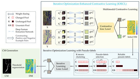
Figure 1. Overall flowchart of proposed IOECL. $x_i$: anchor patch of image X; $x_i^{+}$: positive sample of image X; $x_i^{-}$: negative sample of image X; $y_i$: anchor patch of image Y; $y_i^{+}$: positive sample of image Y; $y_i^{-}$: negative sample of image Y; $O^{x_i}$: features of image X with contrastive learning; $O^{x_i^{+}}$: positive sample features of image X; $O^{x_i^{-}}$: negative sample features of image X; $O^{y_i}$: features of image Y with contrastive learning; $O^{y_i^{+}}$: positive sample features of image Y; $O^{y_i^{-}}$: negative sample features of image Y; ${\Gamma }^X$: features of image X with iterative optimization learning; and ${\Gamma }^Y$: features of image Y with iterative optimization learning.

It is assumed that the multimodal remote sensing images acquired at times t1 and t2 are $X\in {\mathbb{R}}^{W\times H\times C_1}$ and $Y\in {\mathbb{R}}^{W\times H\times C_2}$. They are aligned images of the same region acquired at different times in the image domains $\mathbb{X}$ and $\mathbb{Y}$, respectively. Here, W, H, and $C_1/C_2$ represent the width, height, and number of channels of the images $X/Y$, respectively.

2.1. Deep Feature Extraction Network

To transform multimodal images into a unified deep feature space and derive their representative deep features, a deep feature extraction network is engineered. The network adopts a combination of residual network (ResNet) [51] and feature pyramid network (FPN) [52] architectures, leveraging their multi-scale feature extraction and fusion capacities. The network architecture contains five parts: the general convolution module, the residual convolution, the multi-scale feature fusion, the deconvolution module, and a projection layer.

In an effort to mitigate detail loss typically associated with straightforward downsampling, the network incorporates five general convolution modules. Each of these modules is composed of a single 3 × 3 convolution layer, succeeded by batch normalization and activated via an ReLU function [53]. The mathematical formulation is delineated as follows:

$$m=f\left(bn\right(conv\left(patch\right)\left)\right)$$

(1)

where $conv (·)$ represents convolution functions, $bn (·)$ indicates batch normalization functions and $f (·)$ denotes activation functions.

To simplify the complexity of network learning, images are downsampled using residual convolution [51]. Each residual convolutional unit makes use of skip connections to improve network performance. The residual convolutional unit is computed as follows:

$$m_{l+1}=f(h\left(m_l\right)+\mathrm{F}\left(m_l,W_l\right)),$$

(2)

where $m_l$ and $m_{l+1}$ are the inputs and outputs at layer l, $\mathrm{F}(·)$ is the residual function, $h (·)$ is the constant mapping, and $f(·)$ is the activation function, usually the widely recognized ReLU.

Through the implementation of downsampling operations, features are captured at various scales. To ensure these features encapsulate abundant semantic information, we incorporate an FPN [49] characterized by a top-down architecture augmented with lateral connections. This design facilitates the integration of lower-level, detailed features with higher-level, semantic-rich features, thereby enabling multi-scale feature fusion throughout the extraction process. In order to harmoniously combine features from disparate scales, deconvolution operations are employed to upsample the deep features, resizing them to match the dimensions of the original image patches. Upon separate extraction of deep features from multimodal images, a unified projection layer is introduced to map these features into a shared deep feature space, as depicted in Figure 2. This projection layer is constructed using a single 3 × 3 convolutional layer. Following the unification of deep features, the resultant feature maps from each image layer are designated as $O_1$, $O_2$, and $O_3$, representing the final composite feature representations across differing levels of abstraction.

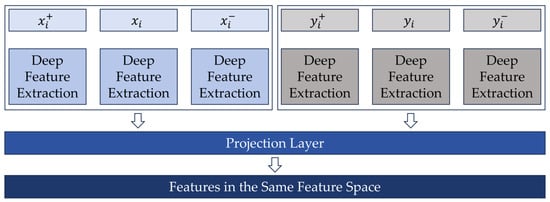
Figure 2. Deep feature unified framework.

Regarding these feature maps, discrepancies exist between deep and shallow features, with each contributing distinctively to the formation of the final feature maps. Consequently, to appropriately account for their varying contributions, feature weights are assigned. The computation of the ultimate output features is thereby conducted according to the following formula:

$$O={\lambda }_1{O}_1+{\lambda }_2{O}_2+{\lambda }_3{O}_3,$$

(3)

where ${\lambda }_1$, ${\lambda }_2$, and ${\lambda }_3$ are the weights of $O_1$, $O_2$, and $O_3$, and ${\lambda }_1+{\lambda }_2+{\lambda }_3=1$. The structure of the deep feature extraction network is shown in Figure 3.

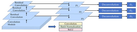
Figure 3. Details of deep feature extraction network.

2.2. Multimodal Contrastive Learning

Contrastive learning entails training a model that, by contrasting semantically equivalent inputs, encourages their proximity within the representation space. A fundamental tactic to avert model collapse involves incorporating dissimilar samples, thereby creating both positive and negative example pairs [54]. This strategic inclusion has found application in several remote sensing studies [55,56,57,58,59].

In our work, we harness contrastive learning augmented with negative sampling to derive deep features. Given a dataset X partitioned into $N$ segments, the ensemble of these segments can be denoted as $\left\{x_i\right|i=1, \dots ,N\}.$ Likewise, the set derived from data Y is constituted as $\left\{y_i\right|i=1, \dots ,N\}.$

Owing to the substantial impact of positive and negative samples on the feature extraction network’s learning efficacy, meticulous selection of these samples is imperative. Consequently, within the same image domain, the patch most similar to the anchor patch is designated as its positive patch, as illustrated in Figure 4. The calculation method for the positive patch is as follows:

$$\left\{\begin{array}{c}{x}_i^{+}=x_{{argmin}_{j \ne i}\left(dist\right(x_i, x_j\left)\right)}\\ y_i^{+}=y_{{argmin}_{j \ne i}\left(dist\right(y_i, y_j\left)\right)}\\ j \ne i;i,j=1, \dots ,N.\end{array}\right.$$

(4)

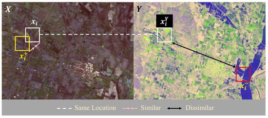
Figure 4. Selection of positive and negative samples. In the $X$ domain, the white box $x_i$ is the anchor patch, and the yellow box $x_i^{+}$ is the positive patch of $x_i$; in the $Y$ domain, the white box $x_i^Y$ is the patch in the same position as the $x_i$ in domain $X$, and the red box $x_i^{-}$ is the negative patch of $x_i$.

Regarding negative samples, they need to represent different objects with some distinctions from the anchor. Here, the negative patch is from another image domain, which is the most dissimilar to the patch consistent with the anchor patch position in another image domain, as shown in Figure 4. The selection of the negative patch is calculated as follows:

$$\left\{\begin{array}{c}{x}_i^{-}=y_{{argmax}_{j \ne i}\left(dist\right(y_i, y_j\left)\right)}\\ y_i^{-}=x_{{argmax}_{j \ne i}\left(dist\right(x_i, x_j\left)\right)}\\ j \ne i;i,j=1, \dots ,N\end{array}\right.,$$

(5)

where $\mathrm{d}\mathrm{i}\mathrm{s}\mathrm{t}\left(\cdot \right)=\sqrt{{‖x_i-x_j‖}^2},j \ne i;i,j=1, \dots ,N$. It is a similarity measurement based on the Euclidean distance.

In summary, the positive and negative pairs for data X are $\{x_i, x_i^{+}\}$ and $\{x_i, x_i^{-}\}$, respectively. Similarly, the positive and negative pairs for data Y are $\{y_i, y_i^{+}\}$ and $\{y_i, y_i^{-}\}$, respectively. This method allows us to focus on the most valuable positive and negative sample information, thereby avoiding the noise introduced by a large number of positive and negative samples in traditional methods.

The proposed IOECL has two major branches, each of which has three minor branches (Figure 1). The anchor patches, positive samples, and negative samples are the inputs to the network branch. Moreover, we propose the contrastive loss function as follows:

$$\begin{gathered} Loss1={\sum }_{c=1}^{C}dist\left(O_c^{x_i}, O_c^{x_i^{+}}\right)+{\sum }_{c=1}^C\mathrm{E}\mathrm{X}\mathrm{P}\left({\displaystyle \frac{{-dist(O}_c^{x_i}, O_c^{x_i^{-}})}{{\lambda }_{1c}}}\right) \\ +{\sum }_{c=1}^{C}dist\left(O_c^{y_i}, O_c^{y_i^{+}}\right)+{\sum }_{c=1}^C\mathrm{E}\mathrm{X}\mathrm{P}\left({\displaystyle \frac{{-dist(O}_c^{y_i}, O_c^{y_i^{-}})}{{\lambda }_{2c}}}\right) \\ \left(C=3\right), \end{gathered}$$

(6)

where C represents deep features acquired at different levels, $O_c^{x_i}$ and $O_c^{y_i}$ represent the cth level features for anchor patches $x_i$ and $y_i$, $O_c^{x_i^{+}}$ and $O_c^{y_i^{+}}$ represent the cth level features for positive samples $x_i^{+}$ and $y_i^{+}$, $O_c^{x_i^{-}}$ and $O_c^{y_i^{-}}$ represent the cth level features for negative samples $x_i^{-}$ and $y_i^{-}$, and $\mathrm{d}\mathrm{i}\mathrm{s}\mathrm{t}(·)$ represents the similarity measurement based on the Euclidean distance. In this paper, ${\lambda }_{1c}$ and ${\lambda }_{2c}$ are set to 3.

If the deep features of the anchor and positive samples are similar, their distance similarity measures converge to 0. Otherwise, when the deep features of the anchor and the negative samples are dissimilar, the distance similarity measure is taken as a negative number and calculated as an exponential function. Therefore, when the differences between the features of the anchor and the negative samples become larger, the loss function is closer to 0. Therefore, the main optimization effects of the loss function are to narrow the distance between the anchor and the positive samples and widen the difference between the anchor and the negative samples.

2.3. Iterative Optimization Learning with Pseudo-Labels

To attain a more consistent and reliable CM, iterative learning is employed to enhance the stability of deep features extracted from bi-temporal images. Striving for a harmony between feature enhancement and learning efficacy, a selective incorporation of dependable pseudo-labels into the iterative training is adopted. This approach serves to fine-tune the network parameters and augment the precision of CD. First, the similarity is measured on the bi-temporal image of the deep features acquired in Section 2.2. The Euclidean distance is then used to measure it and obtain the initial difference map (DM), which is calculated as follows:

$$\mathrm{D}\mathrm{M}=normalize\left(dist\right(O^X, O^Y\left)\right),$$

(7)

where $O^X$ and $O^Y$ are the deep features of the bi-temporal images, respectively. The function $normalize(\cdot )$ refers to the operation of normalizing the data to the range [0, 1] using the formula ${\phi }_i^{\prime }=({\phi }_i-\mathrm{m}\mathrm{i}\mathrm{n}(\phi \left)\right)/(\mathrm{m}\mathrm{a}\mathrm{x}(\phi )-\mathrm{m}\mathrm{i}\mathrm{n}(\phi \left)\right)$. The normalized DM is then clustered into changed, unchanged, and uncertain classes via K-means clustering. This process is denoted as $L=KM(\mathrm{D}\mathrm{M},3)$, with $KM(·)$ denoting the K-means clustering. Following this clustering, the pixels belonging to the changed class and the unchanged class are each sorted separately in descending order of their DM, with $des\left(cl\right)$ representing the sorted changed-class pixels and $des\left(ucl\right)$ denoting the sorted unchanged-class pixels. Subsequently, the changed and unchanged pixels in the top $a\%$ and last $b\%$ are considered as the changed and unchanged pseudo-labels, respectively, and the remainder are classified as uncertain. This approach aids the model in more accurately identifying change areas and prevents overfitting to noise or uncertain regions. The selection of reliable pseudo-labels is defined as follows:

$${RL}_{qs}=\left\{\begin{array}{c}1, L_{qs}>L_{a\%\times des\left(cl\right)}\hfill \\ 0, L_{qs}>L_{b\%\times des\left(ucl\right)}\hfill \\ 2, otherwise\hfill \end{array}\right.,$$

(8)

where $a\%$ and $b\%$ are calculated as:

$$a\%=int\left[\beta \times \left({\displaystyle \frac{ep+1}{ep+2}}\right)\times \mathrm{s}\mathrm{u}\mathrm{m}\left(cl\right)\right]\times 100,$$

(9)

$$b\%=int\left[\beta \times \left({\displaystyle \frac{ep+1}{ep+2}}\right)\times \mathrm{s}\mathrm{u}\mathrm{m}\left(ucl\right)\right]\times 100,$$

(10)

where ${RL}_{qs}$ represents the pseudo-label value for the pixel $(q,s)$; 1, 0, and 2 indicate the labels for the changed, unchanged, and uncertain categories, respectively; $des\left(cl\right)$ and $des\left(ucl\right)$ are the changed and unchanged classes sorted by the values of the DM in descending order, respectively; $sum\left(cl\right)$ and $sum\left(ucl\right)$ indicate the number of pixels in the changed and unchanged categories separately; $ep$ denotes the current iteration count of the network learning process; and $\beta$ is a constant. As the number of iterations increases, the two parameters $a\%$ and $b\%$ also increase, meaning that a higher rate of reliable pseudo-labels is involved in subsequent iterative optimization.

To expand the discrimination between changed and unchanged regions, reliable pseudo-labeled data are involved in iterative optimization learning. Here, we draw upon the contrastive loss [60], with the final learning goal to minimize the loss function. The iterative learning loss function is given by:

$$\begin{gathered} Loss2={\sum }_{q=1}^H{\sum }_{s=1}^W[\left({RL}_{qs}=0\right)\times \mathrm{d}\mathrm{i}\mathrm{s}\mathrm{t}\left({\sum }_{c=1}^C\left(O_c^X\left(q,s\right)-O_c^Y\left(q,s\right)\right)\right) \\ +\left({RL}_{qs}=1\right)\times {\mathrm{m}\mathrm{a}\mathrm{x}(th-\mathrm{d}\mathrm{i}\mathrm{s}\mathrm{t}\left({\sum }_{c=1}^C\left(O_c^X\left(q,s\right)-O_c^Y\left(q,s\right)\right)\right),0)}^2 \\ +\left({RL}_{qs}=2\right)\times \left(1-DM\right)\times \mathrm{d}\mathrm{i}\mathrm{s}\mathrm{t}\left({\sum }_{c=1}^C\left(O_c^X\left(q,s\right)-O_c^Y\left(q,s\right)\right)\right)], \end{gathered}$$

(11)

where C denotes three sets of deep features at different scales, $C=3$ and th = 0.5.

In our study, pseudo-labels are fundamental in the iterative enhancement learning process, especially for differentiating between unchanged and changed regions. Unchanged regions should have similar feature representations, so the distance similarity between these regions should be minimized. For changed regions, when the distance exceeds a predefined threshold th, the value of the function $\mathrm{m}\mathrm{a}\mathrm{x}\left(·\right)$ becomes 0. This indicates that the similarity between anchor samples and negative samples is below the threshold, suggesting that effective differentiation can be achieved without imposing excessive training constraints. In multimodal data, while there may be variations in data representation, the research object remains constant in unchanged regions. Conversely, in changed regions, both the object and its representation may be different. Therefore, deep features in unchanged regions across multimodal images are more stable and consistent compared to those in changed regions. Based on this observation, we constrain the loss between unchanged features to facilitate network learning. To implement this, in Equation (11), we define $(1-DM)$ as the loss weight for the uncertain regions, where the DM is derived from the previous round of learning, with $DM\in [0, 1]$. By assigning higher weights to pixels that are more likely to belong to the unchanged regions, we emphasize the feature differences in the stable features, thereby optimizing the network parameters. Repeating this process allows us to update the reliable pseudo-labels and iteratively refine the network parameters, ultimately leading to higher-quality deep features and improved CD accuracy.

2.4. CM Generation

After the iterative learning of the network, the feature space of the multimodal images is unified, and the bi-temporal features are obtained. Subsequently, these two features are compared using the Euclidean distance to obtain the final DM, which is calculated as

$${DM}_{qs}=\mathrm{d}\mathrm{i}\mathrm{s}\mathrm{t}\left({\Gamma }^X{\left(q,s\right)}^2,{\Gamma }^Y{\left(q,s\right)}^2\right),$$

(12)

where ${\Gamma }^X$ and ${\Gamma }^Y$ are the features of the two images acquired after iterative optimization, and ${DM}_{qs}$ denotes the change intensity of the pixel at $(q,s)$.

To clearly represent the changed and unchanged regions, binary images are obtained. In this paper, we use threshold segmentation to obtain the final CM, which is calculated as:

$${CM}_{qs}=\left\{\begin{array}{c}0, {DM}_{qs}<0.5\\ 1, {DM}_{qs}\ge 0.5\end{array},\right.$$

(13)

where ${CM}_{qs}$ denotes the category (changed or unchanged) of the pixel at $(q,s)$.

3. Experiment and Discussion

In this section, the effectiveness of the proposed IOECL is validated in four sets of multimodal images. The three parameters involved in the experiment are investigated, and their effect on the results is analyzed. In addition, we analyze the differences between the proposed IOECL and other similar methods qualitatively and quantitatively, ensuring an objective assessment of our method.

3.1. Multimodal Datasets and Quantitative Measures

This study utilized four representative datasets to validate the efficacy of the proposed method. These datasets encompass both urban changes (datasets D2 and D3) and riverine changes (datasets D1 and D4). Not only do they cover extensive areas—such as D2, which is 2600 × 4400 pixels—but they also include a diverse array of land cover types. Consequently, these datasets effectively illustrate the performance of the MCD method across various application scenarios.

The California dataset D1 is shown in Figure 5. Image t1 is a Landsat 8 acquisition covering Sacramento County, Yuba County and Sutter County, California, on 5 January 2017. It contains nine bands, shown as a false color image in Figure 5a. Image t2 was acquired on 18 February 2017 by Sentinel-1A over the same area after the occurrence of a flood. The last image is a reference image made by a professional team. The dataset was provided by Luppino et al. [21]. The images are 3500 × 2000 pixels in size and have a spatial resolution of 15 m. This dataset reflects the changes caused by the flood.

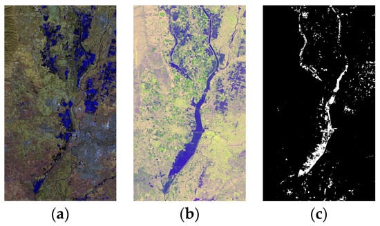
Figure 5. D1: California dataset: (a) image t1; (b) image t2; and (c) ground truth.

Figure 6 (D2) and Figure 7 (D3) show images for Toulouse, France. They depict changes in the built-up areas of the city. Both contain three images, including pre-event, post-event, and reference images. Figure 6a was obtained by TerraSAR-X in February 2009, while Figure 6b was captured by Pleiades in July 2013. Both have a size of 2600 × 4400 pixels and a spatial resolution of 2 m. Meanwhile, Pleiades offered Figure 7a in May 2012, and WorldView 2 provided Figure 7b in July 2013. The two images have a size of 2000 × 2000 and a spatial resolution of 0.52 m.

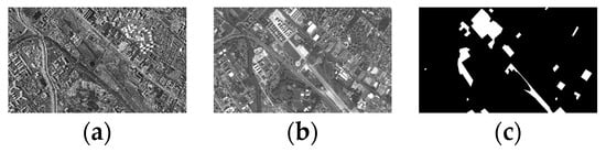
Figure 6. D2: Toulouse dataset: (a) image t1; (b) image t2; and (c) ground truth.

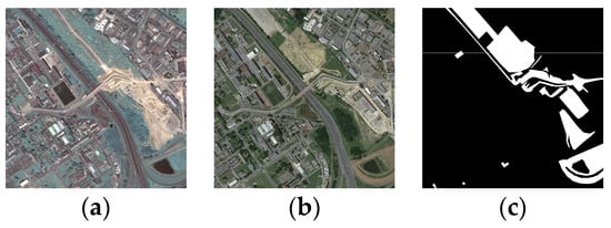
Figure 7. D3: Toulouse dataset: (a) image t1; (b) image t2; and (c) ground truth.

The last dataset, D4, shows flooding in Gloucester, UK (Figure 8). There are three images in D4. The first was acquired by the Spot satellite in 1999, the second is normalized difference vegetation index (NDVI) data obtained in 2000, and the third is a binary change reference map. The images have a size of 990 × 554 pixels and a spatial resolution of 25 m. These data also depict a flood event. The main purpose is to detect flooded areas.

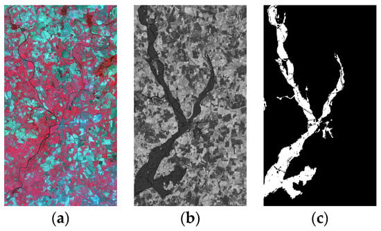
Figure 8. D4: Gloucester dataset: (a) image t1; (b) image t2; and (c) ground truth.

D2, D3, and D4 were provided by Max Mignotte [23].

In order to make the evaluation quantitative, we assessed the performance using the overall accuracy OA, F1 scores F1, and Kappa coefficient k, which are widely used in the accuracy assessment of CD. Their calculation formula is as follows:

(1)

overall accuracy OA:

$$OA={\displaystyle \frac{TP+TN}{TP+TN+FP+FN}},$$

(14)

where TPs, TNs, FPs, and FNs represent the true positives (TP), true negatives (TN), false positives (FP), and false negatives (FN), respectively;

(2)

F1 scores F1:

$$F1={\displaystyle \frac{2·P·R}{P+R}},$$

(15)

$$P={\displaystyle \frac{TP}{TP+FP}},$$

(16)

$$R={\displaystyle \frac{TP}{TP+FN}},$$

(17)

where P and R represent precision and recall, respectively; and

(3)

the Kappa coefficient k:

$$k={\displaystyle \frac{OA-PRE}{1-PRE}},$$

(18)

$$PRE={\displaystyle \frac{\left(TP+FP\right)\times \left(TP+FN\right)+\left(FN+TN\right)\times \left(FP+TN\right)}{{(TP+TN+FP+FN)}^2}}.$$

(19)

Here, the larger the value of k, the higher the precision of CM.

3.2. Experimental Parameter Setting and Analysis

In the experiment, the input image size of D1, D2, and D3 is 128 × 128, and the sample size of D4 is 64 × 64. The experiment is carried out on a Windows system with an NVIDIA GeForce GTX 2080Ti graphics card to enhance training efficiency. The experiment is implemented in Python 3.9.13 using Pytorch 1.12.1. In addition, the remaining parameters are determined through some experiments in the following analysis. In the deep feature extraction network, the convolution and deconvolution sizes are 3 × 3. The activation function used is ReLU, and the Adam optimizer is used in the network training. The learning rate is $lr={10}^{-5}$, and the decay rates of the average gradients are set at $(0.9, 0.999)$. Notably, however, distinct datasets can exhibit divergent sensitivities to uniform parameters. Consequently, calibrating the parameter configuration tailored to individual datasets is vital for augmenting CD accuracy. The proposed IOECL involves examining the influence of the feature fusion coefficients $(O_1,O_2,O_3)$, the iteration control factor ξ, and the sample ratio coefficient β, achieved through a systematic manipulation of variables. Experiments are conducted with diverse combinations of these parameters, and the selection of the optimal parameter set is grounded in the outcomes of these experiments, ensuring a data-driven optimization for improved performance.

3.2.1. Feature Fusion Coefficient $({\mathrm{O}}_1,{\mathrm{O}}_2,{\mathrm{O}}_3)$

In our research, feature fusion is implemented via a weighted combination of features at various depth levels. Shallow-layer features often encompass detailed information, such as edges and textures, whereas deep-layer features tend to capture more abstract concepts, such as object shapes and structures. Rational feature fusion helps retain detailed variations and enhances the model’s comprehension of higher-level feature information, which is vital for multimodal change detection.

To identify the optimal feature fusion strategy, this paper evaluates five distinct configurations of feature fusion coefficients: [1/10, 1/5, 7/10], [1/5, 3/10, 1/2], [1/3, 1/3, 1/3], [1/2, 3/10, 1/5], and [7/10, 1/5, 1/10]. These configurations emphasize different aspects of feature dimensions, aiming to maximize the use of multimodal data information. For example, using the [1/10, 1/5, 7/10] configuration places the highest weight on the top-level feature, which is useful for extracting abstract information, especially for tasks needing a deep understanding of complex patterns. However, this might reduce the capture of detailed information. The [1/3, 1/3, 1/3] configuration equally weighs all three feature levels, seeking a balance among them. This ensures the model does not overly depend on high-level abstract information while also considering low-level detailed features, thus potentially achieving high precision and capturing subtle differences. Adjusting the middle-level feature weights to [1/5, 3/10, 1/2] or [1/2, 3/10, 1/5] has different effects. The first emphasizes the middle-level features, aiding in the use of more abstract information while preserving certain details. The second balances the deep- and shallow-level features, slightly favoring the shallow-level features to improve the detection of local detail changes. Lastly, adopting the [7/10, 1/5, 1/10] configuration focuses on shallow-level features, enhancing the model’s sensitivity to local detail and texture changes. At the same time, other parameters are set to be optimal. The experiment is carried out on the four datasets separately. The obtained overall accuracy OA and the Kappa coefficient k are shown in Figure 9.

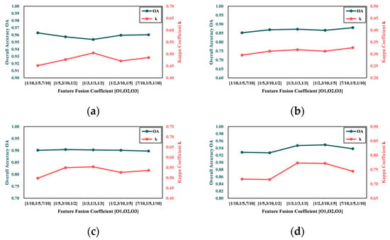
Figure 9. Overall accuracy OA and Kappa coefficient k on CMs with different feature fusion coefficients $(O_1,O_2,O_3)$: (a) D1; (b) D2; (c) D3; and (d) D4.

As is shown in Figure 9, D1, D3, and D4 have the best evaluation results when the feature fusion coefficient is [1/3, 1/3, 1/3], while D2 is less sensitive to this parameter. Overall accuracy OA does not change significantly compared to the Kappa coefficient k on the different parameters, and their change trends remain largely consistent. Since CD does not need to pay attention to the detailed features of the object, the feature fusion parameters are set as [1/3, 1/3, 1/3] for each dataset.

3.2.2. Iteration Coefficient $\mathsf{\xi }$

The number of iterations indicates the number of times that the pseudo-labels is involved in network learning. Too few iterations will reduce the quality of the acquired features, while too many iterations will affect the learning efficiency. The experiments are designed with iteration numbers from 1 to 10. Figure 10 shows the results for the four datasets, illustrating that detection accuracy trends vary with the number of iterations. Specifically, when the number of iterations is six or fewer, the overall accuracy OA and the Kappa coefficient k for datasets D1 to D3 show an upward trend. This indicates that, within a certain range, increasing iterations improves CD accuracy. Further increasing iterations leads to stabilized detection accuracy, possibly because the model has learned sufficient information to distinguish between the changed and unchanged regions, diminishing the benefits of additional iterations. However, on dataset D4, detection accuracy initially decreases when iterations are between one and three, likely due to the low quality of initial pseudo-labels introducing errors, which negatively affects model performance. With increased iterations (from three to six), detection accuracy recovers and stabilizes, suggesting that after an initial “trial-and-error” phase, the model gradually learns more accurate feature representations. After six to ten iterations, detection accuracy remains stable, indicating that the model has converged to a better state. This could be because (1) in the early stages of iteration, pseudo-labels may contain more noise since the model has not yet fully learned to distinguish between the changed and unchanged regions. As the number of iterations increases, the model can gradually correct these errors and improve the quality of the pseudo-labels. A non-robust pseudo-label-generation mechanism may lead to error accumulation, affecting final detection results; (2) dataset D4 may contain more complex change patterns or higher noise levels, making it easier for the model to be disturbed during the early stages of iteration. However, as the model continues to learn, it can gradually overcome these challenges and improve detection accuracy. Based on the above analysis, the number of iterations for each dataset is set as six.

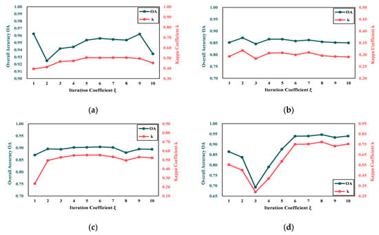
Figure 10. Overall accuracy OA and Kappa coefficient k on CMs with different iterations $\xi$: (a) D1; (b) D2; (c) D3; and (d) D4.

3.2.3. Sample Ratio Coefficient $\mathsf{\beta }$

The sample ratio coefficient $\beta$ is crucial for controlling the proportion of reliable samples to total samples. If the coefficient is too small, more prior information cannot be provided, making the optimization process longer and more difficult. And the final CMs will be inaccurate because insufficient useful prior information makes it hard to enhance the difference between changed and unchanged regions. If the coefficient is too large, more incorrect prior information will be introduced, which will not be effective for optimization learning and will reduce the accuracy of the final result. Therefore, in this paper, the sample ratio coefficient $\beta$ is set from 1/20 to 5/10 in steps of 1/10. As can be seen in Figure 11, D2 is less sensitive to this parameter than other datasets. However, for D1, D3, and D4, the optimum value of the sample ratio coefficient $\beta$ is 1/10, 3/10, and 1/10, respectively. Based on the above analysis, the sample ratio coefficient $\beta$ is set to be less than 3/10 in this paper.

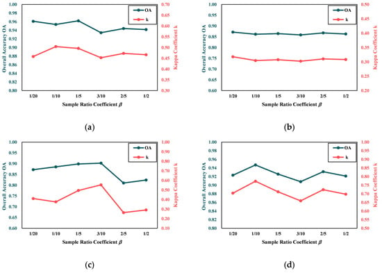
Figure 11. Overall accuracy OA and Kappa coefficient k on CMs with different sample ratio coefficient $\beta$: (a) D1; (b) D2; (c) D3; and (d) D4.

Taking D3 as an example, as shown in Figure 12, the blue, red, and green bars in the table indicate the number of changed (C), unchanged (UC), and unsure (US) categories of reliable pseudo-labels. The gray line shows the trend of the ratio of reliable pseudo-labels to the total number of labels. It can be seen that the number of changed and unchanged labels increases dynamically with the increase in iterations, and a higher percentage of accurate information is provided to assist in network optimization and obtain more accurate detection results. The differences between the changed and unchanged regions are significantly enhanced after the pseudo-labels are involved in several iterations of training, verifying the effectiveness of the pseudo-label dynamic update method proposed in this paper.

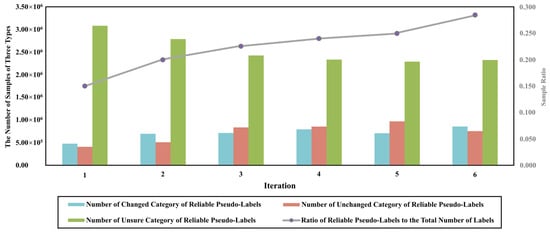
Figure 12. Number of changed (C), unchanged (UC), and unsure (US) categories of reliable pseudo-labels, and trend of ratio of reliable pseudo-labels to total number of labels.

3.3. Performance of Proposed IOECL and Comparison Methods

In order to evaluate the proposed method properly, unsupervised learning methods, namely the SCCN [42], X-Net [47], ACE-Net [47], CAN [45], nonlocal patch similarity-based graph (NPSG) [27], improved nonlocal patch-based graph (INLPG) [32], iterative robust graph, Markovian co-segmentation method (IRG-McS) [31], and sparse-constrained adaptive structure consistency (SCASC) [32], are chosen for comparison. To ensure fair evaluation, we carry out the comparison methods on each dataset using the optimal settings of the key parameters (Table 1).

Table 1. Optimal settings of the key parameters for each comparison method.

SCCN	Weighting parameter $\lambda =0.15$; learning rate is ${10}^{-4}$; and the number of epochs is 500.
X-Net	Dropout rate is 20%; loss function for 240 epochs at a learning rate of ${10}^{-5}$; and the weights of the loss functions are three: $w_{cyc}=2$, $w_{\alpha }=3$, and $w_{\theta }=0.001$.
ACE-Net	Dropout rate is 20%; loss function for 240 epochs at a learning rate of ${10}^{-5}$; and the weights of the loss functions are five: $w_{adv}=2$, $w_{AE}=0.2$,$w_{cyc}=2$, $w_{\alpha }=3$, and $w_{\theta }=0.001.$
CAN	Weighting parameter $\lambda =5$; learning rate is ${10}^{-4}$; and the number of epochs is 500.
NPSG	Patch size $p_s=5$; search window size ${\xi }_s=20p_s$; search step size ${\mathsf{\Delta }}_s=2$; target patch step size ${\mathsf{\Delta }}_p=3$; and the selected most similar neighbors $K=35$.
INLPG	Patch size $p=2$; step size ${\mathsf{\Delta }}_p=2$; and the most similar neighbors $K=0.01N$ (N is the total number of patches).
IRG-McS	Superpixels number $N_S=\mathrm{10,000}$; and the maximum number of iterations $Iter=6$.
SCASC	Superpixels number $N_S=\mathrm{10,000}$; and weighting parameter $\lambda =0.1$.

The performance of different methods on each dataset is evaluated as follows:

(1)

Experiments on D1: The CMs and accuracy evaluation of D1 are shown in Figure 13 and Table 2, respectively. Generally speaking, these methods achieved relatively ideal results in changed-area detection. Most methods detected relatively complete flooding areas. This is due to the obvious difference between flooding areas and the background of image t2. However, since the changed areas are relatively small above the image, it is easy to mix in unchanged fragment information while detecting changed areas. Compared with CAN, the proposed method relatively completely retains the detailed outline of changed areas. In addition, the proposed method minimizes the detection of unchanged areas as changed areas compared with the remaining eight methods. This is mainly due to the iterative optimization, which uses reliable pseudo-labels to enhance the distinction between changed and unchanged areas.

From the accuracy evaluation, the proposed method has a great advantage with a Kappa coefficient k of 0.5025. The overall accuracy OA and F1 scores F1 are 0.9560 and 0.5255, respectively, both of which also have significant accuracy improvements.

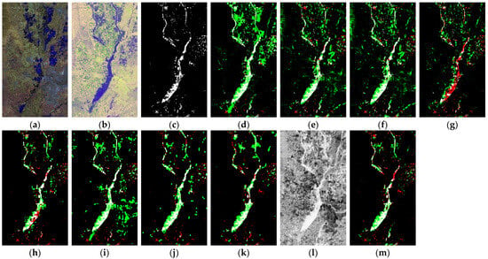
Figure 13. CD results on D1: (a) Image t1; (b) Image t2; (c) Ground truth; (d) SCCN; (e) X-Net; (f) ACE-Net; (g) CAN; (h) NPSG; (i) INLPG; (j) IRG-McS; (k) SCASC; (l) DM of IOECL; and (m) CM of IOECL. White: TPs; green: FPs; black: TNs; and red: FNs.

Table 2. Quantitative evaluation of CD results of proposed method compared to other methods on D1. (Highest values are in bold.)

Method	P	R	OA	F1	k
SCCN	0.2872	0.9050	0.8977	0.4360	0.3960
X-Net	0.2735	0.7273	0.9008	0.3975	0.3566
ACE-Net	0.2613	0.7272	0.8982	0.3845	0.3422
CAN	0.2739	0.3590	0.9304	0.3107	0.2748
NPSG	0.4263	0.5411	0.9481	0.4769	0.4500
INLPG	0.3002	0.7309	0.9138	0.4256	0.3876
IRG-McS	0.4040	0.6542	0.9427	0.4995	0.4709
SCASC	0.4117	0.6181	0.9447	0.4942	0.4662
IOECL	0.4966	0.5579	0.9560	0.5255	0.5025

(2)

Experiments on D2: The CMs of different methods on dataset D2 are shown in Figure 14. As can be seen from Table 3, due to the large number of small and fragmented buildings, the accuracy of the nine methods on these data is relatively low. The accuracy of SCASC is slightly higher than that of the method proposed in this paper.

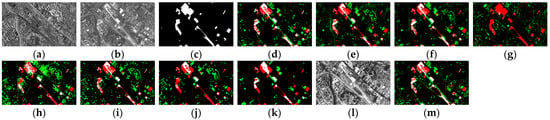Figure 14. CD results on D2: (a) Image t1; (b) Image t2; (c) Ground truth; (d) SCCN; (e) X-Net; (f) ACE-Net; (g) CAN; (h) NPSG; (i) INLPG; (j) IRG-McS; (k) SCASC; (l) DM of IOECL; and (m) CM of IOECL d. White: TPs; green: FPs; black: TNs; and red: FNs.

Table 3. Quantitative evaluation of CD results of proposed method compared to other methods on D2. (Highest values are in bold.)

Method	P	R	OA	F1	k
SCCN	0.3767	0.5434	0.8922	0.4449	0.3874
X-Net	0.2551	0.3527	0.8609	0.2961	0.2211
ACE-Net	0.3244	0.4119	0.8801	0.3630	0.2978
CAN	0.0410	0.0334	0.8610	0.0368	−0.0373
NPSG	0.1974	0.3919	0.8249	0.2625	0.1753
INLPG	0.2744	0.4036	0.8677	0.3267	0.2562
IRG-McS	0.2678	0.2867	0.8809	0.2769	0.2122
SCASC	0.4748	0.4072	0.9170	0.4384	0.3939
IOECL	0.2866	0.5289	0.8578	0.3717	0.2995

The main reason is that SCASC reduces the false detection of changed areas as much as possible. Compared with the other eight methods, the proposed method has more obvious advantages. In particular, regarding the scattered building area in the upper right-hand corner, the X-Net, ACE-Net, NPSG, INLPG, and IRG-McS detect it as a changed area. The proposed method uses a stable feature extraction network to achieve stable deep features, reducing similar false detection. From this point and the automaticity of the proposed method, the feature extraction network proposed in this paper shows greater advantages.

(3)

Experiments on D3: Figure 15 shows two high-resolution optical images acquired from different satellite sensors. The proposed method has far fewer false detections compared to the other eight methods and detects the most complete changed area in the semi-circular part at the bottom of the changed building area. In terms of accuracy evaluation (Table 4), the proposed method obtains the highest Kappa coefficient k of 0.5533, which is much higher than those of the other comparison methods. Its overall accuracy OA and F1 scores F1 both achieved the best results of 0.9040 and 0.6041, respectively. The proposed method has such good performance on this dataset for two main reasons: The data have higher spatial resolutions, and their detailed information provides a database for obtaining more accurate feature information, while iterative optimization plays a very important role in expanding the differences between the changed and unchanged regions of the image, significantly improving the accuracy of the data after several iterations of optimization.

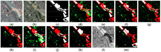Figure 15. CD results on D3: (a) Image t1; (b) Image t2; (c) Ground truth; (d) SCCN; (e) X-Net; (f) ACE-Net; (g) CAN; (h) NPSG; (i) INLPG; (j) IRG-McS; (k) SCASC; (l) DM of IOECL; and (m) CM of IOECL. White: TPs; green: FPs; black: TNs; and red: FNs.

Table 4. Quantitative evaluation of CD results of proposed method compared to other methods on D3. (Highest values are in bold).

Method	P	R	OA	F1	k
SCCN	0.3380	0.2604	0.8106	0.2942	0.1869
X-Net	0.5827	0.3980	0.8583	0.4729	0.3944
ACE-Net	0.5929	0.3137	0.8560	0.4103	0.3370
CAN	0.4606	0.2161	0.8428	0.2942	0.2185
NPSG	0.4692	0.1218	0.8460	0.1934	0.1397
INLPG	0.4003	0.4289	0.8160	0.4141	0.3051
IRG-McS	0.6022	0.2829	0.8630	0.3849	0.3189
SCASC	0.8015	0.4041	0.8945	0.5373	0.4849
IOECL	0.8054	0.4833	0.9040	0.6041	0.5533

(4)

Experiments on D4: The geographical features of D4 are simple, and the proposed method also achieves the best detection results of F1 scores F1 and the Kappa coefficient k. By observing the results shown in Figure 16, it is clear that the proposed method detects the changed area more completely than the other four comparison methods, the SCCN, INLPG, IRG-McS, and SCASC. However, the existence of many small fragments in the unchanged area, which are relatively complex and could easily be mistakenly divided into changed areas, poses a challenge for this dataset. The method proposed here has fewer false detections than the other methods in the unchanged areas. From Table 5, we can see that the proposed method achieved an overall accuracy OA, F1 score F1, and Kappa coefficient k of 0.9393, 0.7849, and 0.7505, respectively, which are relatively better than those of the other methods. With step-by-step iterative optimization, the changed features gradually become more obvious, and the contours of the changed regions gradually become clearer, distinctly distinguishing them from the unchanged regions. Therefore, better results are achieved in the final results. Compared to other methods, the iterative optimization part of the proposed method shows great advantages in strengthening the features of the changed regions and reducing fragmented false detections.

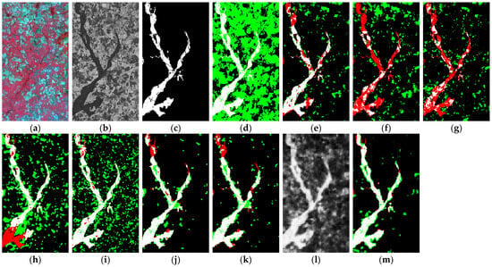Figure 16. CD results on D4: (a) Image t1; (b) Image t2; (c) Ground truth; (d) SCCN; (e) X-Net; (f) ACE-Net; (g) CAN; (h) NPSG; (i) INLPG; (j) IRG-McS; (k) SCASC; (l) DI of IOECL; and (m) CM of IOECL. White: TPs; green: FPs; black: TNs; and red: FNs.

Table 5. Quantitative evaluation of CD results of proposed method compared to other methods on D4. (Highest values are in bold).

Method	P	R	OA	F1	k
SCCN	0.1662	0.9998	0.4016	0.2850	0.1011
X-Net	0.6041	0.7361	0.9110	0.6636	0.6129
ACE-Net	0.2492	0.2737	0.8150	0.2609	0.1554
CAN	0.3310	0.2891	0.8455	0.3086	0.2221
NPSG	0.3123	0.6684	0.7849	0.4257	0.3142
INLPG	0.3886	0.9386	0.8166	0.5497	0.4583
IRG-McS	0.6997	0.8685	0.9399	0.7750	0.7408
SCASC	0.6763	0.8202	0.9317	0.7413	0.7024
IOECL	0.6801	0.9278	0.9393	0.7849	0.7505

3.4. Ablation Study

The proposed method is mainly divided into two parts: deep learning based on contrastive learning and iterative optimization learning. In order to examine the effects of these two parts, results with and without iteration optimization of the four datasets are compared, as shown in Figure 17 and Table 6. Although result accuracy without iteration is not optimistic, the general outline of the changed area is relatively obvious, as shown in Figure 17a. It shows that the deep feature space unification is successful through the proposed network. It also plays a positive role in selecting reliable pseudo-labels to guide iterative optimization. The accuracy of four datasets has been improved after iterative optimization. As shown in Figure 17a,b, the changed areas have been significantly enhanced after iterative optimization. The differences between the changed and unchanged areas have also been enlarged. Figure 17 takes D3 as an example to show the effects of iteration optimization from step to step. The final accuracy of the results shows obvious improvement, as shown in Table 6.

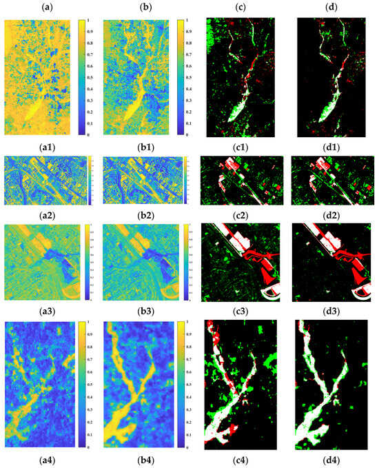
Figure 17. Results with and without iteration optimization of the four datasets—(a): (a1–a4) DMs for datasets D1–D4 without iteration optimization; (b): (b1–b4) DMs for datasets D1–D4 with iteration optimization; (c): (c1–c4) CMs for datasets D1–D4 without iteration optimization; and (d): (d1–d4) CMs for datasets D1–D4 with iteration optimization. White: TPs; red: FPs; black: TNs; and green: FNs.

Table 6. Quantitative evaluation of CMs with and without iteration optimization. (Highest values are in bold).

Iteration	D1			D2			D3			D4
	OA	F1	k	OA	F1	k	OA	F1	k	OA	F1	k
0	0.9029	0.3089	0.2646	0.8626	0.3623	0.2912	0.8464	0.5142	0.4231	0.8783	0.5846	0.5162
6	0.9560	0.5255	0.5025	0.8578	0.3717	0.2995	0.9040	0.6041	0.5533	0.9393	0.7849	0.7505

4. Conclusions

The proposed IOECL establishes a pathway between multimodal datasets using a deep feature unification network grounded in contrastive learning. By doing so, this approach transforms two distinct images into a shared feature space, enabling direct and effective comparison. The dynamic acquisition of pseudo-labels facilitates the automatic renewal of reliable pseudo-labels throughout the iterative learning process. This mechanism aims to provide high-quality and accurate labels for the optimization process, thereby accelerating network optimization. To further refine the model, an optimized loss function is designed for regions experiencing changes, unchanged regions, and uncertain regions, thereby optimizing network parameters accordingly. This process aids in obtaining higher-quality features in the two temporal images and better final CMs. Based on the proposed method’s performance across four datasets and comparative analysis with similar methods, the proposed IOECL demonstrates advantages in addressing the problem of MCD.

While the proposed method demonstrated commendable performance in experiments, there are also some limitations. The optimal parameters for the proposed IOECL are derived from extensive experimentation. Future work will develop an automated hyperparameter tuning mechanism to efficiently identify the best hyperparameter combinations for specific tasks. For dynamic pseudo-label selection, we utilized a classic and simple K-means clustering algorithm. Future research could explore more advanced clustering methods to refine the pseudo-label learning mechanism, improving pseudo-label quality through finer rules and considering adaptive learning rates or other optimization strategies to minimize the accumulation of erroneous information.

To achieve long-term, large-scale, multi-class dynamic monitoring, we aim to enhance the model’s generalization and robustness to adapt to varying scenarios. Specifically, transfer learning can leverage pre-trained models to accelerate the adaptation to new datasets. A multi-task learning framework can share underlying feature representations, improving the model’s ability to detect multiple types of changes. Incorporating online learning mechanisms will enable the model to update in real time, adapting to changes in data streams. These algorithmic improvements will facilitate efficient and accurate MCD across a wide range of monitoring tasks, including land use changes, forest cover changes, flood monitoring, post-earthquake CD, road damage detection, and surveillance of facilities such as airports, ports, etc.

References

- Tang, Y.; Zhang, L. Urban Change Analysis with Multi-Sensor Multispectral Imagery. Remote Sens. 2017, 9, 252. [Google Scholar] [CrossRef]
- Chen, Y.; Tang, Y.; Han, T.; Zhang, Y.; Zou, B.; Feng, H. RAMC: A Rotation Adaptive Tracker with Motion Constraint for Satellite Video Single-Object Tracking. Remote Sens. 2022, 14, 3108. [Google Scholar] [CrossRef]
- Chen, Y.; Tang, Y.; Yin, Z.; Han, T.; Zou, B.; Feng, H. Single Object Tracking in Satellite Videos: A Correlation Filter-Based Dual-Flow Tracker. IEEE J. Sel. Top. Appl. Earth Obs. Remote Sens. 2022, 15, 6687–6698. [Google Scholar] [CrossRef]
- Han, T.; Tang, Y.; Yang, X.; Lin, Z.; Zou, B.; Feng, H. Change Detection for Heterogeneous Remote Sensing Images with Improved Training of Hierarchical Extreme Learning Machine (HELM). Remote Sens. 2021, 13, 4918. [Google Scholar] [CrossRef]
- Hussain, M.; Chen, D.; Cheng, A.; Wei, H.; Stanley, D. Change Detection from Remotely Sensed Images: From Pixel-Based to Object-Based Approaches. ISPRS J. Photogramm. Remote Sens. 2013, 80, 91–106. [Google Scholar] [CrossRef]
- Wu, C.; Du, B.; Zhang, L. Fully Convolutional Change Detection Framework with Generative Adversarial Network for Unsupervised, Weakly Supervised and Regional Supervised Change Detection. IEEE Trans. Pattern Anal. Mach. Intell. 2023, 45, 9774–9788. [Google Scholar] [CrossRef] [PubMed]
- Zhang, M.; Zhang, R.; Yang, Y.; Bai, H.; Zhang, J.; Guo, J. ISNet: Shape Matters for Infrared Small Target Detection. In Proceedings of the 2022 IEEE/CVF Conference on Computer Vision and Pattern Recognition (CVPR), New Orleans, LA, USA, 18–24 June 2022; pp. 867–876. [Google Scholar]
- Zhang, M.; Bai, H.; Zhang, J.; Zhang, R.; Wang, C.; Guo, J.; Gao, X. RKformer: Runge-Kutta Transformer with Random-Connection Attention for Infrared Small Target Detection. In Proceedings of the 30th ACM International Conference on Multimedia, Lisboa, Portugal, 10 October 2022; pp. 1730–1738. [Google Scholar]
- Chen, Y.; Yuan, Q.; Tang, Y.; Xiao, Y.; He, J.; Han, T.; Liu, Z.; Zhang, L. SSTtrack: A Unified Hyperspectral Video Tracking Framework via Modeling Spectral-Spatial-Temporal Conditions. Inf. Fusion 2025, 114, 102658. [Google Scholar] [CrossRef]
- Zhang, M.; Yue, K.; Li, B.; Guo, J.; Li, Y.; Gao, X. Single-Frame Infrared Small Target Detection via Gaussian Curvature Inspired Network. IEEE Trans. Geosci. Remote Sens. 2024, 62, 5005013. [Google Scholar] [CrossRef]
- Zhang, M.; Wang, Y.; Guo, J.; Li, Y.; Gao, X.; Zhang, J. IRSAM: Advancing Segment Anything Model for Infrared Small Target Detection. arXiv 2024, arXiv:2407.07520. [Google Scholar]
- Yang, J.; Zhou, Y.; Cao, Y.; Feng, L. Heterogeneous Image Change Detection Using Deep Canonical Correlation Analysis. In Proceedings of the 2018 24th International Conference on Pattern Recognition (ICPR), Beijing, China, 20–24 August 2018; pp. 2917–2922. [Google Scholar]
- Zhou, Y.; Liu, H.; Li, D.; Cao, H.; Yang, J.; Li, Z. Cross-Sensor Image Change Detection Based on Deep Canonically Correlated Autoencoders. In Artificial Intelligence for Communications and Networks; Han, S., Ye, L., Meng, W., Eds.; Lecture Notes of the Institute for Computer Sciences, Social Informatics and Telecommunications Engineering; Springer International Publishing: Cham, Switzerland, 2019; Volume 286, pp. 251–257. ISBN 978-3-030-22967-2. [Google Scholar]
- Shao, R.; Du, C.; Chen, H.; Li, J. SUNet: Change Detection for Heterogeneous Remote Sensing Images from Satellite and UAV Using a Dual-Channel Fully Convolution Network. Remote Sens. 2021, 13, 3750. [Google Scholar] [CrossRef]
- Zhang, C.; Feng, Y.; Hu, L.; Tapete, D.; Pan, L.; Liang, Z.; Cigna, F.; Yue, P. A Domain Adaptation Neural Network for Change Detection with Heterogeneous Optical and SAR Remote Sensing Images. Int. J. Appl. Earth Obs. Geoinf. 2022, 109, 102769. [Google Scholar] [CrossRef]
- Zhang, M.; Zhang, R.; Zhang, J.; Guo, J.; Li, Y.; Gao, X. Dim2Clear Network for Infrared Small Target Detection. IEEE Trans. Geosci. Remote Sens. 2023, 61, 4700718. [Google Scholar] [CrossRef]
- Ma, W.; Xiong, Y.; Wu, Y.; Yang, H.; Zhang, X.; Jiao, L. Change Detection in Remote Sensing Images Based on Image Mapping and a Deep Capsule Network. Remote Sens. 2019, 11, 626. [Google Scholar] [CrossRef]
- Liu, H.; Wang, Z.; Shang, F.; Zhang, M.; Gong, M.; Ge, F.; Jiao, L. A Novel Deep Framework for Change Detection of Multi-Source Heterogeneous Images. In Proceedings of the 2019 International Conference on Data Mining Workshops (ICDMW), Beijing, China, 8–11 November 2019; pp. 165–171. [Google Scholar]
- Jiang, X.; Li, G.; Zhang, X.-P.; He, Y. A Semisupervised Siamese Network for Efficient Change Detection in Heterogeneous Remote Sensing Images. IEEE Trans. Geosci. Remote Sens. 2022, 60, 4700718. [Google Scholar] [CrossRef]
- Shi, J.; Wu, T.; Qin, A.K.; Lei, Y.; Jeon, G. Semisupervised Adaptive Ladder Network for Remote Sensing Image Change Detection. IEEE Trans. Geosci. Remote Sens. 2022, 60, 5408220. [Google Scholar] [CrossRef]
- Luppino, L.T.; Bianchi, F.M.; Moser, G.; Anfinsen, S.N. Unsupervised Image Regression for Heterogeneous Change Detection. IEEE Trans. Geosci. Remote Sens. 2019, 57, 9960–9975. [Google Scholar] [CrossRef]
- Gong, M.; Zhang, P.; Su, L.; Liu, J. Coupled Dictionary Learning for Change Detection from Multisource Data. IEEE Trans. Geosci. Remote Sens. 2016, 54, 7077–7091. [Google Scholar] [CrossRef]
- Mignotte, M. A Fractal Projection and Markovian Segmentation-Based Approach for Multimodal Change Detection. IEEE Trans. Geosci. Remote Sens. 2020, 58, 8046–8058. [Google Scholar] [CrossRef]
- Jimenez-Sierra, D.A.; Benítez-Restrepo, H.D.; Vargas-Cardona, H.D.; Chanussot, J. Graph-Based Data Fusion Applied to: Change Detection and Biomass Estimation in Rice Crops. Remote Sens. 2020, 12, 2683. [Google Scholar] [CrossRef]
- Han, T.; Tang, Y.; Zou, B.; Feng, H. Unsupervised Multimodal Change Detection Based on Adaptive Optimization of Structured Graph. Int. J. Appl. Earth Obs. Geoinf. 2024, 126, 103630. [Google Scholar] [CrossRef]
- Han, T.; Tang, Y.; Chen, Y.; Zou, B.; Feng, H. Global Structure Graph Mapping for Multimodal Change Detection. Int. J. Digit. Earth 2024, 17, 2347457. [Google Scholar] [CrossRef]
- Sun, Y.; Lei, L.; Li, X.; Sun, H.; Kuang, G. Nonlocal Patch Similarity Based Heterogeneous Remote Sensing Change Detection. Pattern Recognit. 2021, 109, 107598. [Google Scholar] [CrossRef]
- Zhao, L.; Sun, Y.; Lei, L.; Zhang, S. Auto-Weighted Structured Graph-Based Regression Method for Heterogeneous Change Detection. Remote Sens. 2022, 14, 4570. [Google Scholar] [CrossRef]
- Tang, Y.; Yang, X.; Han, T.; Zhang, F.; Zou, B.; Feng, H. Enhanced Graph Structure Representation for Unsupervised Heterogeneous Change Detection. Remote Sens. 2024, 16, 721. [Google Scholar] [CrossRef]
- Sun, Y.; Lei, L.; Li, X.; Tan, X.; Kuang, G. Structure Consistency-Based Graph for Unsupervised Change Detection with Homogeneous and Heterogeneous Remote Sensing Images. IEEE Trans. Geosci. Remote Sens. 2022, 60, 4700221. [Google Scholar] [CrossRef]
- Sun, Y.; Lei, L.; Guan, D.; Kuang, G. Iterative Robust Graph for Unsupervised Change Detection of Heterogeneous Remote Sensing Images. IEEE Trans. Image Process. 2021, 30, 6277–6291. [Google Scholar] [CrossRef] [PubMed]
- Sun, Y.; Lei, L.; Guan, D.; Li, M.; Kuang, G. Sparse-Constrained Adaptive Structure Consistency-Based Unsupervised Image Regression for Heterogeneous Remote-Sensing Change Detection. IEEE Trans. Geosci. Remote Sens. 2022, 60, 4405814. [Google Scholar] [CrossRef]
- Han, T.; Tang, Y.; Chen, Y.; Yang, X.; Guo, Y.; Jiang, S. SDC-GAE: Structural Difference Compensation Graph Autoencoder for Unsupervised Multimodal Change Detection. IEEE Trans. Geosci. Remote Sens. 2024, 62, 5622416. [Google Scholar] [CrossRef]
- Rani, V.; Nabi, S.T.; Kumar, M.; Mittal, A.; Kumar, K. Self-Supervised Learning: A Succinct Review. Arch. Computat. Methods Eng. 2023, 30, 2761–2775. [Google Scholar] [CrossRef]
- Gui, J.; Chen, T.; Zhang, J.; Cao, Q.; Sun, Z.; Luo, H.; Tao, D. A Survey on Self-Supervised Learning: Algorithms, Applications, and Future Trends. IEEE Trans. Pattern Anal. Mach. Intell. 2023, 1–20. [Google Scholar] [CrossRef]
- Liu, X.; Zhang, F.; Hou, Z.; Mian, L.; Wang, Z.; Zhang, J.; Tang, J. Self-Supervised Learning: Generative or Contrastive. IEEE Trans. Knowl. Data Eng. 2021, 35, 857–876. [Google Scholar] [CrossRef]
- Bond-Taylor, S.; Leach, A.; Long, Y.; Willcocks, C.G. Deep Generative Modelling: A Comparative Review of VAEs, GANs, Normalizing Flows, Energy-Based and Autoregressive Models. IEEE Trans. Pattern Anal. Mach. Intell. 2022, 44, 7327–7347. [Google Scholar] [CrossRef] [PubMed]
- Kingma, D.P.; Welling, M. An Introduction to Variational Autoencoders. FNT Mach. Learn. 2019, 12, 307–392. [Google Scholar] [CrossRef]
- Wang, K.; Gou, C.; Duan, Y.; Lin, Y.; Zheng, X.; Wang, F.-Y. Generative Adversarial Networks: Introduction and Outlook. IEEE/CAA J. Autom. Sinica 2017, 4, 588–598. [Google Scholar] [CrossRef]
- Gui, J.; Sun, Z.; Wen, Y.; Tao, D.; Ye, J. A Review on Generative Adversarial Networks: Algorithms, Theory, and Applications. IEEE Trans. Knowl. Data Eng. 2023, 35, 3313–3332. [Google Scholar] [CrossRef]
- Han, T.; Tang, Y.; Chen, Y. Heterogeneous Image Change Detection Based on Two-Stage Joint Feature Learning. In Proceedings of the IGARSS 2022–2022 IEEE International Geoscience and Remote Sensing Symposium, Kuala Lumpur, Malaysia, 17–22 July 2022; pp. 3215–3218. [Google Scholar]
- Liu, J.; Gong, M.; Qin, K.; Zhang, P. A Deep Convolutional Coupling Network for Change Detection Based on Heterogeneous Optical and Radar Images. IEEE Trans. Neural Netw. Learn. Syst. 2018, 29, 545–559. [Google Scholar] [CrossRef]
- Zhao, W.; Wang, Z.; Gong, M.; Liu, J. Discriminative Feature Learning for Unsupervised Change Detection in Heterogeneous Images Based on a Coupled Neural Network. IEEE Trans. Geosci. Remote Sens. 2017, 55, 7066–7080. [Google Scholar] [CrossRef]
- Su, L.; Gong, M.; Zhang, P.; Zhang, M.; Liu, J.; Yang, H. Deep Learning and Mapping Based Ternary Change Detection for Information Unbalanced Images. Pattern Recognit. 2017, 66, 213–228. [Google Scholar] [CrossRef]
- Niu, X.; Gong, M.; Zhan, T.; Yang, Y. A Conditional Adversarial Network for Change Detection in Heterogeneous Images. IEEE Geosci. Remote Sens. Lett. 2019, 16, 45–49. [Google Scholar] [CrossRef]
- Zhan, T.; Gong, M.; Jiang, X.; Li, S. Log-Based Transformation Feature Learning for Change Detection in Heterogeneous Images. IEEE Geosci. Remote Sens. Lett. 2018, 15, 1352–1356. [Google Scholar] [CrossRef]
- Luppino, L.T.; Kampffmeyer, M.; Bianchi, F.M.; Moser, G.; Serpico, S.B.; Jenssen, R.; Anfinsen, S.N. Deep Image Translation with an Affinity-Based Change Prior for Unsupervised Multimodal Change Detection. IEEE Trans. Geosci. Remote Sens. 2022, 60, 4700422. [Google Scholar] [CrossRef]
- Chen, Y.; Bruzzone, L. Self-Supervised Change Detection in Multiview Remote Sensing Images. IEEE Trans. Geosci. Remote Sens. 2022, 60, 5402812. [Google Scholar] [CrossRef]
- Saha, S.; Ebel, P.; Zhu, X.X. Self-Supervised Multisensor Change Detection. IEEE Trans. Geosci. Remote Sens. 2022, 60, 4405710. [Google Scholar] [CrossRef]
- Hartigan, J.A.; Wong, M.A. Algorithm AS 136: A K-Means Clustering Algorithm. Appl. Stat. 1979, 28, 100. [Google Scholar] [CrossRef]
- He, K.; Zhang, X.; Ren, S.; Sun, J. Deep Residual Learning for Image Recognition. In Proceedings of the 2016 IEEE Conference on Computer Vision and Pattern Recognition (CVPR), Las Vegas, NV, USA, 27–30 June 2016; pp. 770–778. [Google Scholar]
- Lin, T.-Y.; Dollar, P.; Girshick, R.; He, K.; Hariharan, B.; Belongie, S. Feature Pyramid Networks for Object Detection. In Proceedings of the 2017 IEEE Conference on Computer Vision and Pattern Recognition (CVPR), Honolulu, HI, USA, 21–26 July 2017; pp. 936–944. [Google Scholar]
- Agarap, A.F. Deep Learning Using Rectified Linear Units (ReLU). arXiv 2019, arXiv:1803.08375. [Google Scholar]
- Wang, Y.; Albrecht, C.M.; Braham, N.A.A.; Mou, L.; Zhu, X.X. Self-Supervised Learning in Remote Sensing: A Review. IEEE Geosci. Remote Sens. Mag. 2022, 10, 213–247. [Google Scholar] [CrossRef]
- Zhang, L.; Lu, W.; Zhang, J.; Wang, H. A Semisupervised Convolution Neural Network for Partial Unlabeled Remote-Sensing Image Segmentation. IEEE Geosci. Remote Sens. Lett. 2022, 19, 6507305. [Google Scholar] [CrossRef]
- Yang, J.; Kang, Z.; Yang, Z.; Xie, J.; Xue, B.; Yang, J.; Tao, J. A Laboratory Open-Set Martian Rock Classification Method Based on Spectral Signatures. IEEE Trans. Geosci. Remote Sens. 2022, 60, 4601815. [Google Scholar] [CrossRef]
- Rao, W.; Qu, Y.; Gao, L.; Sun, X.; Wu, Y.; Zhang, B. Transferable Network with Siamese Architecture for Anomaly Detection in Hyperspectral Images. Int. J. Appl. Earth Obs. Geoinf. 2022, 106, 102669. [Google Scholar] [CrossRef]
- Jing, H.; Cheng, Y.; Wu, H.; Wang, H. Radar Target Detection with Multi-Task Learning in Heterogeneous Environment. IEEE Geosci. Remote Sens. Lett. 2022, 19, 4021405. [Google Scholar] [CrossRef]
- Zhang, L.; Zhang, S.; Zou, B.; Dong, H. Unsupervised Deep Representation Learning and Few-Shot Classification of PolSAR Images. IEEE Trans. Geosci. Remote Sens. 2022, 60, 5100316. [Google Scholar] [CrossRef]
- Schroff, F.; Kalenichenko, D.; Philbin, J. FaceNet: A Unified Embedding for Face Recognition and Clustering. In Proceedings of the 2015 IEEE Conference on Computer Vision and Pattern Recognition (CVPR), Boston, MA, USA, 7–12 June 2015; pp. 815–823. [Google Scholar]
Disclaimer/Publisher’s Note: The statements, opinions and data contained in all publications are solely those of the individual author(s) and contributor(s) and not of MDPI and/or the editor(s). MDPI and/or the editor(s) disclaim responsibility for any injury to people or property resulting from any ideas, methods, instructions or products referred to in the content. |
© 2024 by the authors. Licensee MDPI, Basel, Switzerland. This article is an open access article distributed under the terms and conditions of the Creative Commons Attribution (CC BY) license (https://creativecommons.org/licenses/by/4.0/).