Robust Underwater Direction-of-Arrival Estimation Method Using Acoustic Sensor Array under Unknown Swing Deviation Elements

Abstract

This paper presents a strategy called the alternating iterative minimization method (AIMM), aimed at enhancing the precision of direction of arrival (DOA) estimation when utilizing an acoustic vector sensor array (AVSA) with unknown swing deviation elements (SDEs). The AVSA model with unknown SDEs is formulated by incorporating the swing deviation parameter. Later, to estimate the swing deviation matrix (SDM) and the sparse signal power by using the alternating iteration method, the auxiliary cost functions with respect to SDM and the sparse signal power are formulated based on the regularized weighted least squares (RWLS) and regularized covariance matrix fitting (RCMF) criteria. Furthermore, their analytical expressions have also been quantified. In order to mitigate the effect of unknown SDEs on the accuracy of DOA estimation, any sub-time segment (STS) in the dataset is selected as the reference to convert the received data of different STS into the reference STS using the estimated SDM. The simulation and experimental outcomes conclusively represent the effectiveness of the suggested TSIM approach using AVSA in handling unknown SDEs.

1. Introduction

Direction of arrival (DOA) estimates are very meaningful and practical for target locating in passive acoustic systems. The acoustic vector sensor (AVS) consists of scalar and orthogonal dipole elements, allowing it to simultaneously collect sound pressure and acoustic particle velocity (APV) data, as mentioned in [1,2,3]. By utilizing additional acoustic data, one AVS is able to accurately determine the DOA of acoustic sources without left–right ambiguity in the entire spatial range in contrast to an acoustic scalar sensor (ASS) [4]. Moreover, the AVS array (AVSA) has the ability to offer significant advantages over individual AVSs in terms of interference suppression and spatial resolution [5,6]. Thus, the AVS or AVSA is widely used in many fields, for example, radar, microphone, sonar, and wireless communication systems [7,8,9,10,11,12,13,14].

Subspace-based algorithms, such as conventional beamforming (CBF) [15], minimum variance distortionless response (MVDR) [16], multiple signal classification (MUSIC) [17], and their variants [4,18,19], have been utilized for DOA estimation. It is well known that they have high spatial resolution when dealing with uncorrelated sources, a significant amount of snaphots, and large signal-to-noise ratio (SNR). On the other hand, in practical applications, acquiring enough snapshots may be a difficult task, particularly in rapidly changing and intricate underwater environments, which may be have a considerable impact on the precision of estimating the DOA. The ${\ell }_1$-norm-based singular value decomposition (L1SVD) technique proposed in [20], which is a classical sparse reconstruction method, can achieve high-precision DOA estimation in scenarios with correlated sources, low SNR, and few snapshots. However, the selection of suitable regularization parameters is a challenge. To mitigate this issue, a sparse asymptotic minimum variance (SAMV) technique without setting user parameters is formulated in [21]. Most of the above methods have been applied to DOA estimation of a single AVS or AVSA and and have been validated in underwater environments [15,18,22,23]. The results show that these methods can all achieve direction-of-arrival estimation of underwater sources. But they ignore the sparse characteristic of signal in the spatial field, which may lead to a low spatial resolution at low SNR. To overcome this problem, the weighted power iterative compensation (WPIC) technique, relying on the sparse covariance matrix fitting criterion, is proposed in [24] to enhance the resolution performance of DOA estimation. The underwater experimental results show that compared with MUSIC, SAMV, and L1SVD, by designing a weight with user parameters to compensate for signal power and enhance its sparsity in the spatial domain, the WPIC method has the strongest ability to suppress interference and noise. Moreover, to overcome the situation where the AVS receives ambient noise instead of internal noise in underwater environments, resulting in unequal noise power of sound pressure and APV sensors, a DOA estimation method based on MUSIC for asymptotically eliminating environmental noise is proposed in [25], which transformed the array covariance matrix into a new covariance matrix with noise concentrated in the real part, and improved the estimation performance of underwater DOA under low SNR. However, these algorithms mentioned previously rely on the premise that the AVSA is a uniform linear array. As reported in [26], sparse arrays, including coprime arrays [27,28] and nested arrays [29,30], are originally presented for the ASS array. Compared to the uniform linear array, they are capable of resolving a greater number of sources than the number of physical sensors. In recent years, a large number of improved sparse AVSAs have been developed in [31,32,33,34] to enhance the DOA estimation accuracy. Furthermore, deep learning has found extensive application in DOA estimation. Compared to subspace and sparse methods, deep learning approaches exhibit remarkable advantages in DOA estimation [35]. As stated in [35], the DOA estimation process is performed online after offline training of the network, resulting in relatively lower computational complexity compared to sparse methods. In [36], an improved convolutional neural network method has been proposed to estimate the DOA of underwater acoustic by using a two-channel convolutional neural network with a real and virtual covariance matrix as the input signal of the convolutional neural network. The experimental results demonstrate that the improved convolutional neural network method achieves higher accuracy and estimation efficiency in underwater acoustic environments with low SNR. In [37], the DOA estimation problem is transformed into a neural network classification problem, and underwater DOA estimation methods of convolutional neural networks and long short-term memory networks are proposed. However, most of the deep learning approaches construct their models for DOA estimation based on the ASS arrays. However, the application of deep learning specifically tailored for AVSAs remains scarce. In [38], a deep transfer learning method using a single AVS for DOA estimation is formulated by training a convolutional neural network using synthetic data in the source domain. By combining long-term DOA estimation with short-term memory and an attention mechanism, an improved deep learning DOA estimation method is also proposed in [39].

It is noted that most of the DOA estimation performed by the aforementioned method is based on the ideal linear array. However, in real-world applications, sensors and their arrays exhibit high sensitivity to model errors, for example, sensor position errors, gain/phase errors, and the axial angle deviation that we commonly encounter [40,41]. The performance of the aforementioned methods can be significantly degraded under the influence of model errors. By using labor-intensive and expensive calibration procedures to eliminate the effects of gain/phase errors, these mismatches have been corrected in [42,43]. However, these methods are impractical for numerous sensors. The study in [44] proposes a new method to reduce the variance by increasing the microphone spacing and then using the proposed bias model to remove the angular bias to mitigate the angular bias due to the limited microphone distance in AVS. Furthermore, [45] presents a calibration method for a custom AVS that corrects microphone amplitude and phase in stages. In [46], a three-step iterative algorithm is adopted to estimate the gain and phase error using a space-matching filter, and then a maximum posterior exercise is performed to further adjust the estimated phase parameters and source direction of the underwater three-dimensional sonar imaging system. In addition, based on maximum likelihood and maximum a posteriori approaches, the gain/phase errors are determined in [47,48]. In addition to gain/phase errors and sensor position errors, the AVSAs often face axial angle deviation due to installation errors and the inherent directionality of AVS. To address this challenge, leveraging the unique structural attributes of the axial deviation matrix, an alternating iterative adaptive approach tailored for uniform AVS linear arrays has been presented in [49]. Moreover, eigenstructure-based DOA estimation algorithms are developed in [50] to improve the performance of DOA estimation using a circular AVS array under axial deviation. It is worth noting that these methods mentioned in [49,50] are analyzed under the assumption that the velocity axis points in the same direction for each observation STS. This is due to the fact that these methods are based on the assumption that the axial angle deviation remains constant throughout the observation period. However, in fact, the AVS and external support are typically coupled by springs and other flexible components. Consequently, the direction of the AVSA may swing randomly due to the influence of facts such as ocean current, sea wave, and squalls. In this case, the data collected by the AVSA are likely to have unknown swing deviation elements (SDEs), leading to a significant deterioration in DOA estimation performance. To tackle this challenge, by selecting an appropriate reference STS and then focusing the other STS to the reference STS through the covariance matrix focusing technology, a covariance matrix focusing fitting (CMFF) algorithm is introduced in [51], aimed at mitigating the detrimental effects of unknown SDE factors on the accuracy of DOA estimation. What cannot be ignored is that selecting the reference STS is a challenge. In addition, the influence of the noise covariance matrix is not considered when using covariance matrix focusing technology, which leads to inaccurate DOA estimation at low SNR.

In this paper, we present an alternating iterative minimization method (AIMM) to tackle the aforementioned challenges. To begin with, the data model of AVSA with unknown SDEs is established by incorporating swing deviation parameters into different STSs. Furthermore, by using the criteria of the regularized weighted least squares (RWLS) and regularized covariance matrix fitting (RCMF), we formulate cost functions for swing deviation parameters and sparse signal power. Then, we utilize the estimated swing deviation matrix (SDM) to convert the received data at different STSs to the reference STS, thereby reducing the effect of unkown SDE on DOA estimation performance. In the end, we perform a spectral peaks search on the magnitude of a sparse signal in order to determine the DOA. Extensive numerical simulations and lake-based experimental outcomes have demonstrated that compared with the existing algorithms for an AVSA with unknown SDE, the proposed method achieves robustness and high-precision DOA estimation.

Notation: ${\mathbf{B}}^T$, ${\mathbf{B}}^H$, and ${\mathbf{B}}^{†}$ are the transpose, conjugate transpose, and pseudo-inverse operations of matrix $\mathbf{B}$, respectively. $diag(·)$ and $blkdiag(·)$ correspond to the operations of diagonalization and block diagonalization, respectively. The superscript j of ${(·)}^{\left(j\right)}$ represents the j-th iterative. $Tr\{·\}$ is the trace operation of the matrix. ⊗ signifies the application of the Kronecker product. ${∥·∥}_F$ represents the Frobenious norm operation. ${\mathbf{E}}_M$ indicates the $M\times M$ identity matrix.

2. Problem Description

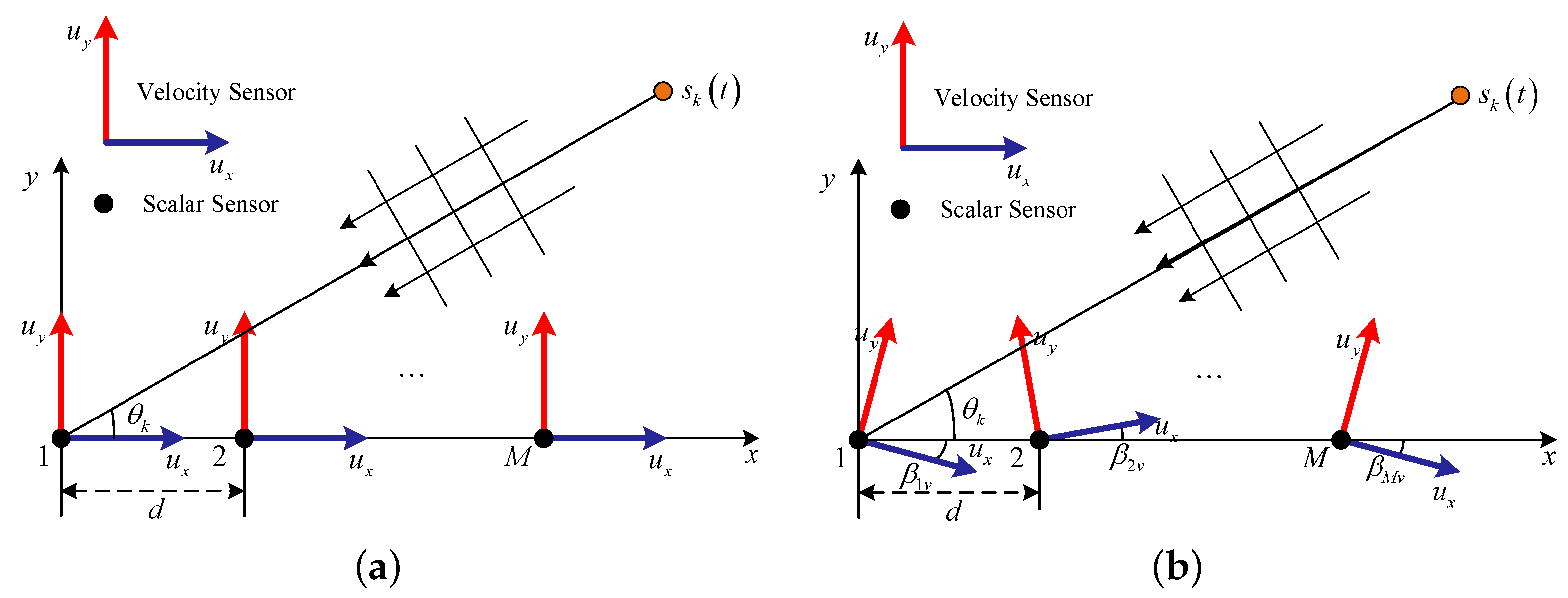
2.1. The Ideal Model of AVSA

We assume K far-field narrow-band sources ${\left\{s_k\right\}}_{k=1}^K$ from directions of $\mathit{\theta }={\left[{\theta }_1,{\theta }_2,\cdots ,{\theta }_K\right]}^T$ incident on a uniform linear array of m component AVSs, which comprise two orthogonal APV sensors and one ASS in every AVS, as shown in Figure 1a, where d is the element spacing, and $u_x$ and $u_y$ denote the mutually orthogonal APV component of AVS, respectively. The received signal vector at time t can be expressed as

$$\mathbf{y}\left(t\right)=\mathbf{A}\left(\mathit{\theta }\right)\mathbf{s}\left(t\right)+\mathbf{w}\left(t\right),$$

(1)

where $\mathbf{y}\left(t\right)={[y_1\left(t\right),y_2\left(t\right),\cdots ,y_{3M}\left(t\right)]}^T$ is the output vector, $\mathbf{s}\left(t\right)={[s_1\left(t\right),s_2\left(t\right),\cdots ,s_K\left(t\right)]}^T$ is the source, $\mathbf{w}\left(t\right)={[w_1\left(t\right),w_2\left(t\right),\cdots ,w_{3M}\left(t\right)]}^T$ denotes the complex independent white Gaussian noise with zero mean, and $\mathbf{A}\left(\mathit{\theta }\right)=[\mathbf{a}\left({\theta }_1\right),\mathbf{a}\left({\theta }_2\right),\cdots ,\mathbf{a}\left({\theta }_K\right)]$ is the manifold matrix of the AVSA, and note that $\mathbf{a}\left({\theta }_k\right)$, which is the manifold vector of the k-th source, can be respresented as

$$\mathbf{a}\left({\theta }_k\right)={[a_{1p}\left({\theta }_k\right)\otimes \mathbf{h}\left({\theta }_k\right),\cdots ,a_{Mp}\left({\theta }_k\right)\otimes \mathbf{h}\left({\theta }_k\right)]}^T$$

(2)

where $\mathbf{h}\left({\theta }_k\right)={\left[1 cos{\theta }_k sin{\theta }_k\right]}^T$ represents the manifold vector of a single AVS, $a_{mp}\left({\theta }_k\right)=e^{-j2\pi \left(\frac{(M-1)d}{\lambda }\right)cos{\theta }_k}$ being the acoustic pressure response coefficient, and $\lambda$ denoting the signal wavelength.

2.2. The Model of AVSA with SDE

With the assumption that L snapshots are collected by AVSA for the entire observation duration, then the number of snapshots collected during the entire observation duration can be divided into V STSs of equal length. Let $\mathcal{L}$ be the snapshot of every single STS, and then we can obtain $\mathcal{L}={\displaystyle \frac{L}{V}}$. It is obvious that the data for each STS are collected with the APV axis of the AVSA pointing in the same direction if the AVSA is in a stationary state throughout the entire observation duration. However, in complex underwater environments, the APV axes of the AVSA may experience random swings during the observation period due to factors such as buoyancy, hydrodynamic effects, and gales, resulting in different SDEs in each STS, and the swing deviation element of each STS is usually difficult to obtain. In this case, the measurement model of AVSA under swing deviation element in the v-th STS is described in Figure 1b, while ${\beta }_{mv}$ describes the unknown SDEs in the v-th STS for the m-th AVS. Then, the manifold matrix of the m-th AVS for the k-th signal source in the v-th STS is denoted by

$$\begin{array}{cc}\hfill \mathbf{h}({\theta }_k,{\beta }_{mv})& =\left[\begin{array}{c}1\\ cos({\theta }_k-{\beta }_{mv})\\ sin({\theta }_k-{\beta }_{mv})\end{array}\right]\hfill \\ \hfill & =\left[\begin{array}{c}1\\ cos{\theta }_{k}cos{\beta }_{mv}+sin{\theta }_{k}sin{\beta }_{mv}\\ sin{\theta }_{k}cos{\beta }_{mv}-cos{\theta }_{k}sin{\beta }_{mv}\end{array}\right]\hfill \\ \hfill & ={\mathbf{g}}_{mv}\mathbf{h}\left({\theta }_k\right)\hfill \end{array}$$

(3)

with

$${\mathbf{g}}_{mv}=\left[\begin{array}{ccc}1& 0& 0\\ 0& cos{\beta }_{mv}& sin{\beta }_{mv}\\ 0& -sin{\beta }_{mv}& cos{\beta }_{mv}\end{array}\right].$$

(4)

Based on (4), we can obtain

$${\mathbf{g}}_{mv}{\mathbf{g}}_{mv}^H={\mathbf{g}}_{mv}^H{\mathbf{g}}_{mv}={\mathbf{E}}_3.$$

(5)

Let ${\mathit{\beta }}_v=\left[{\beta }_{1v},{\beta }_{2v},\cdots ,{\beta }_{Mv}\right]$ be the unknown SDE vector of AVSA in the v-th STS. Then, the manifold matrix of the AVSA can be expressed as

$$\begin{array}{cc}\hfill \mathbf{A}\left(\mathit{\theta },{\mathit{\beta }}_v\right)& ={\left[\mathbf{a}\left({\theta }_1,{\mathit{\beta }}_v\right),\cdots ,\mathbf{a}\left({\theta }_K,{\mathit{\beta }}_v\right)\right]}^T\hfill \\ \hfill & ={[{\mathbf{G}}_v\mathbf{a}\left({\theta }_1\right),\cdots ,{\mathbf{G}}_v\mathbf{a}\left({\theta }_K\right)]}^T\hfill \\ \hfill & ={\mathbf{G}}_v\mathbf{A}\left(\mathit{\theta }\right),\hfill \end{array}$$

(6)

where ${\mathbf{G}}_v\in {\mathbb{C}}^{3M\times 3M}$, which represents the SDM of AVSA in the v-th STS, is written by

$${\mathbf{G}}_v=blkdiag\left\{{\mathbf{g}}_{1v},{\mathbf{g}}_{2v},\cdots ,{\mathbf{g}}_{Mv}\right\}=\left[\begin{array}{cccc}{\mathbf{g}}_{1v}& \mathbf{0}& \cdots & \mathbf{0}\\ \mathbf{0}& {\mathbf{g}}_{2v}& \cdots & \mathbf{0}\\ ⋮& ⋮& \ddots & \mathbf{0}\\ \mathbf{0}& \mathbf{0}& \cdots & {\mathbf{g}}_{Mv}\end{array}\right].$$

(7)

Define $L_s$ as the duration between each sample. Then, the output vector of AVSA during the v-th STS is represented by

$${\mathbf{Y}}_v={\mathbf{G}}_v\mathbf{A}\left(\mathit{\theta }\right){\mathbf{S}}_v+{\mathbf{W}}_v,$$

(8)

where ${\mathbf{Y}}_v=\left[{\mathbf{y}}_v\left(L_s\right),{\mathbf{y}}_v\left(2L_s\right),\cdots ,{\mathbf{y}}_v\left(\mathcal{L}{L}_s\right)\right]\in {\mathbb{C}}^{3M\times \mathcal{L}}$, ${\mathbf{S}}_v=\left[{\mathbf{s}}_v\left(L_s\right),{\mathbf{s}}_v\left(2L_s\right),\cdots ,{\mathbf{s}}_v\left(\mathcal{L}{L}_s\right)\right]\in {\mathbb{C}}^{K\times \mathcal{L}}$ is the signal vector, and ${\mathbf{W}}_v=\left[{\mathbf{w}}_v\left(L_s\right),{\mathbf{w}}_v\left(2L_s\right),\cdots ,{\mathbf{w}}_v\left(\mathcal{L}{L}_s\right)\right]\in {\mathbb{C}}^{3M\times \mathcal{L}}$ represents the Guassian noise vector with zero mean.

It is supposed that the spatial domain is partitioned into N discrete grids, where N is much greater than K. The possible angles of arrival can be mathematically denoted by $\tilde{\mathit{\theta }}=\left\{{\tilde{\theta }}_1,{\tilde{\theta }}_2,\cdots ,{\tilde{\theta }}_N\right\}$. Moreover, we use the assumption that the DOAs of the sources are situated inside distinct matrices, i.e., ${\left\{{\theta }_k\right\}}_{k=1}^K\in \tilde{\mathit{\theta }}$. Subsequently, (8) can be reformulated by

$${\mathbf{Y}}_v={\mathbf{G}}_v\mathbf{A}\left(\tilde{\mathit{\theta }}\right){\tilde{\mathbf{S}}}_v+{\mathbf{W}}_v.$$

(9)

During the entire observation time, the output vector of AVSA with unknown SDEs is shown as

$$\mathbf{Y}=\left[{\mathbf{Y}}_0,{\mathbf{Y}}_1,\cdots ,{\mathbf{Y}}_v,\cdots ,{\mathbf{Y}}_{V-1}\right].$$

(10)

From (9) and (10), we observe that the output data of the AVSA with unknown SDEs match the ideal case when ${\mathbf{G}}_v=\mathbf{E}$. However, when ${\mathbf{G}}_v\ne \mathbf{E}$, the array manifold matrix for receiving data in each STS of AVSA differs. Consequently, directly using the received data over the entire observation period, as in Equation (10), to determine the DOA could result in significant performance degradation.

3. The Proposed Technique

In this section, an AIMM is proposed to estimate the SDM of AVSA ${\left\{{\mathbf{G}}_v\right\}}_{v=0}^{V-1}$ and the sparse signal power ${\left\{{\tilde{\mathbf{p}}}_v\right\}}_{v=0}^{V-1}$ with the alternating iteration method for each STS in the following subsection.

3.1. Estimating the SDM

The singular value decomposition of observation data in the v-th STS is written by

$$\begin{array}{cc}\hfill {\mathbf{Y}}_v& ={\mathbf{U}}_v{\Sigma }_v{\mathbf{Z}}_v^H\hfill \\ \hfill & ={\mathbf{U}}_{Sv}{\Sigma }_{Sv}{\mathbf{Z}}_{Sv}^H+{\mathbf{U}}_{Wv}{\Sigma }_{Wv}{\mathbf{Z}}_{Wv}^H,\hfill \end{array}$$

(11)

where ${\Sigma }_v$ denotes a diagonal matrix consisting of the singular values as diagonal elements, and ${\mathbf{U}}_{Wv}$ and ${\mathbf{Z}}_{Wv}$ represent the noise subspace and the corresponding right singular value vector matrix, respectively. Therefore, the output vector corresponding to the noise subspace is given by

$${\mathbf{Y}}_{Wv}={\mathbf{Y}}_v{\mathbf{Z}}_{Wv}.$$

(12)

In the first step, based on the RWLS technique, the auxiliary function for the SDM is presented, where we keep the sparse signal fixed,

$${\mathbf{G}}_v^{(j+1)}=argminF\left({\mathbf{G}}_v\right)$$

(13)

with

$$F\left({\mathbf{G}}_v^{(j+1)}\right)={∥{\mathbf{Y}}_{Wv}^{†\left(j\right)}({\mathbf{Y}}_v^{\left(j\right)}-{\mathbf{G}}_v\mathbf{A}\left(\tilde{\mathit{\theta }}\right){\tilde{\mathbf{S}}}_v^{\left(j\right)})∥}_F^2+\psi {∥{\mathbf{G}}_v∥}_F^q,$$

(14)

where $\psi >0$ serves as a regularization parameter, adjusting the balance between the weighted least squares component and the Frobenius norm terms, and $0<q\le 1$ is a user-defined parameter utilized to impose constraints on the efficiency of the swing deviation matrix solution.

Note that it is challenging to solve for ${\mathbf{G}}_v$ from (14) due to the nonlinearity introduced by the user parameter q. To overcome this difficulty, let $\mathcal{H}\left(x\right)=x^{\frac{q}{2}}$, and $x={∥{\mathbf{G}}_v∥}_F^2$ and $x_0={∥{\mathbf{G}}_v^{\left(j\right)}∥}_F^2$. As stated in [52], the following inequality is constant:

$$\mathcal{H}\left(x\right)\le \mathcal{H}\left(x_0\right)+{\mathcal{H}}^{\prime }\left(x_0\right)\left(x-x_0\right).$$

(15)

Then, substituting $x={∥{\mathbf{G}}_v∥}_F^2$ and $x_0={∥{\mathbf{G}}_v^{\left(j\right)}∥}_F^2$ into the function $\mathcal{H}\left(x\right)=x^{\frac{q}{2}}$, we hold

$$\begin{array}{cc}\hfill {\left({∥{\mathbf{G}}_v∥}_F^2\right)}^{\frac{q}{2}}& \le {\left({∥{\mathbf{G}}_v^{\left(j\right)}∥}_F^2\right)}^{\frac{q}{2}}\hfill \\ \hfill & +\frac{q}{2}{\left({∥{\mathbf{G}}_v^{\left(j\right)}∥}_F^2\right)}^{\left(\frac{q}{2}-1\right)}\left({∥{\mathbf{G}}_v∥}_F^2-{∥{\mathbf{G}}_v^{\left(j\right)}∥}_F^2\right).\hfill \end{array}$$

(16)

Multiplying $\psi$ and then adding ${∥{\mathbf{Y}}_{W0}^{†}({\mathbf{Y}}_v-{\mathbf{G}}_v\mathbf{A}\left(\tilde{\mathit{\theta }}\right){\tilde{\mathbf{S}}}_v)∥}_F^2$ on both sides of (16), we obtain

$$\mathcal{H}\left({\mathbf{G}}_v\right)\le H\left({\mathbf{G}}_v\right)$$

(17)

with

$$\begin{array}{cc}\hfill H\left({\mathbf{G}}_v\right)& ={∥{\mathbf{Y}}_{W0}^{†}({\mathbf{Y}}_v-{\mathbf{G}}_v\mathbf{A}\left(\tilde{\mathit{\theta }}\right){\tilde{\mathbf{S}}}_v)∥}_F^2+\psi {\left({∥{\mathbf{G}}_v^{\left(j\right)}∥}_F^2\right)}^{\frac{q}{2}}\hfill \\ \hfill & +\psi \frac{q}{2}{\left({∥{\mathbf{G}}_v^{\left(j\right)}∥}_F^2\right)}^{\left(\frac{q}{2}-1\right)}\left({∥{\mathbf{G}}_v∥}_F^2-{∥{\mathbf{G}}_v^{\left(j\right)}∥}_F^2\right).\hfill \end{array}$$

(18)

It is interesting to note that ${\mathbf{G}}_v^{\left(j\right)}$ represents the estimation result of ${\mathbf{G}}_v$ in the j-th iteration. Thus, ${\mathbf{G}}_v^{\left(j\right)}$ is known in (18). Then, (13) can be further transformed into

$${\mathbf{G}}_v^{(j+1)}=argminF\left({\mathbf{G}}_v\right)$$

(19)

with

$$\begin{array}{cc}\hfill F\left({\mathbf{G}}_v\right)& ={∥{\mathbf{Y}}_{W0}^{†}({\mathbf{Y}}_v^{\left(j\right)}-{\mathbf{G}}_v\mathbf{A}\left(\tilde{\mathit{\theta }}\right){\tilde{\mathbf{S}}}_v^{\left(j\right)})∥}_F^2\hfill \\ \hfill & +\psi \frac{q}{2}{\left({∥{\mathbf{G}}_v^{\left(j\right)}∥}_F^2\right)}^{\left(\frac{q}{2}-1\right)}{∥{\mathbf{G}}_v∥}_F^2.\hfill \end{array}$$

(20)

According to the Frobenius norm properties, (20) can be given as

$$\begin{array}{cc}\hfill & F\left({\mathbf{G}}_v\right)=\frac{q\psi }{2}{\left({∥{\mathbf{G}}_v^{\left(j\right)}∥}_F^2\right)}^{\left(\frac{q}{2}-1\right)}Tr\left\{{\mathbf{G}}_v^H{\mathbf{G}}_v\right\}+\hfill \\ & Tr\left\{{\left({\mathbf{Y}}_{W0}^{†}({\mathbf{Y}}_v-{\mathbf{G}}_v\mathbf{A}\left(\tilde{\mathit{\theta }}\right){\tilde{\mathbf{S}}}_v)\right)}^H\left({\mathbf{Y}}_{W0}^{†}({\mathbf{Y}}_v-{\mathbf{G}}_v\mathbf{A}\left(\tilde{\mathit{\theta }}\right){\tilde{\mathbf{S}}}_v)\right)\right\}\hfill \\ \hfill & =Tr\left\{{\mathbf{Y}}_v^H{\left({\mathbf{Y}}_{W0}^{†}\right)}^H{\mathbf{Y}}_{W0}^{†}{\mathbf{Y}}_v\right\}\hfill \\ \hfill & -2Tr\left\{{\mathbf{Y}}_v^H{\left({\mathbf{Y}}_{W0}^{†}\right)}^H{\mathbf{Y}}_{W0}^{†}{\mathbf{G}}_v\mathbf{A}\left(\tilde{\mathit{\theta }}\right){\tilde{\mathbf{S}}}_v\right\}\hfill \\ \hfill & +Tr\left\{{\tilde{\mathbf{S}}}_v^H{\mathbf{A}}^H\left(\tilde{\mathit{\theta }}\right){\mathbf{G}}_v^H{\left({\mathbf{Y}}_{W0}^{†}\right)}^H{\mathbf{Y}}_{W0}^{†}{\mathbf{G}}_v\mathbf{A}\left(\tilde{\mathit{\theta }}\right){\tilde{\mathbf{S}}}_v\right\}\hfill \\ \hfill & +\frac{q{\lambda }_s}{2}{\left({∥{\mathbf{G}}_v^{\left(j\right)}∥}_F^2\right)}^{\left(\frac{q}{2}-1\right)}Tr\left\{{\mathbf{G}}_v^H{\mathbf{G}}_v\right\}.\hfill \end{array}$$

(21)

We now present the first-order differential expressions for the second, third, and last terms of (21) with respect to ${\mathbf{G}}_v$. Utilizing matrix derivative properties, we maintain

$$\begin{array}{cc}\hfill & \mathcal{D}\left(Tr\left\{{\mathbf{Y}}_v^H{\left({\mathbf{Y}}_{W0}^{†}\right)}^H{\mathbf{Y}}_{W0}^{†}{\mathbf{G}}_v\mathbf{A}\left(\tilde{\mathit{\theta }}\right){\tilde{\mathbf{S}}}_v\right\}\right)\hfill \\ \hfill & =Tr\left\{{\mathbf{Y}}_v^H{\left({\mathbf{Y}}_{W0}^{†}\right)}^H{\mathbf{Y}}_{W0}^{†}\mathcal{D}\left({\mathbf{G}}_v\right)\mathbf{A}\left(\tilde{\mathit{\theta }}\right){\tilde{\mathbf{S}}}_v\right\}\hfill \\ \hfill & =Tr\left\{\mathbf{A}\left(\tilde{\mathit{\theta }}\right){\tilde{\mathbf{S}}}_v{\mathbf{Y}}_v^H{\left({\mathbf{Y}}_{W0}^{†}\right)}^H{\mathbf{Y}}_{W0}^{†}\mathcal{D}\left({\mathbf{G}}_v\right)\right\},\hfill \end{array}$$

(22)

$$\begin{array}{cc}\hfill & \mathcal{D}\left(Tr\left\{{\tilde{\mathbf{S}}}_v^H{\mathbf{A}}^H\left(\tilde{\mathit{\theta }}\right){\mathbf{G}}_v^H{\left({\mathbf{Y}}_{Wv}^{†}\right)}^H{\mathbf{Y}}_{Wv}^{†}{\mathbf{G}}_v\mathbf{A}\left(\tilde{\mathit{\theta }}\right){\tilde{\mathbf{S}}}_v\right\}\right)\hfill \\ \hfill & =Tr\left\{{\tilde{\mathbf{S}}}_v^H{\mathbf{A}}^H\left(\tilde{\mathit{\theta }}\right)\mathcal{D}\left({\mathbf{G}}_v^H\right){\left({\mathbf{Y}}_{Wv}^{†}\right)}^H{\mathbf{Y}}_{Wv}^{†}{\mathbf{G}}_v\mathbf{A}\left(\tilde{\mathit{\theta }}\right){\tilde{\mathbf{S}}}_v\right\}\hfill \\ \hfill & +Tr\left\{{\tilde{\mathbf{S}}}_v^H{\mathbf{A}}^H\left(\tilde{\mathit{\theta }}\right){\mathbf{G}}_v^H{\left({\mathbf{Y}}_{W0}^{†}\right)}^H{\mathbf{Y}}_{W0}^{†}\mathcal{D}\left({\mathbf{G}}_v\right)\mathbf{A}\left(\tilde{\mathit{\theta }}\right){\tilde{\mathbf{S}}}_v\right\}\hfill \\ \hfill & =Tr\left\{\mathbf{A}\left(\tilde{\mathit{\theta }}\right){\tilde{\mathbf{S}}}_v{\tilde{\mathbf{S}}}_v^H{\mathbf{A}}^H\left(\tilde{\mathit{\theta }}\right){\mathbf{G}}_v^H{\left({\mathbf{Y}}_{W0}^{†}\right)}^H{\mathbf{Y}}_{W0}^{†}\mathcal{D}\left({\mathbf{G}}_v\right)\right\}\hfill \\ \hfill & +Tr\left\{\mathbf{A}\left(\tilde{\mathit{\theta }}\right){\tilde{\mathbf{S}}}_v{\tilde{\mathbf{S}}}_v^H{\mathbf{A}}^H\left(\tilde{\mathit{\theta }}\right){\mathbf{G}}_v^H{\left({\mathbf{Y}}_{W0}^{†}\right)}^H{\mathbf{Y}}_{W0}^{†}\mathcal{D}\left({\mathbf{G}}_v\right)\right\},\hfill \end{array}$$

(23)

and

$$\begin{array}{cc}\hfill & \mathcal{D}\left(\frac{q\psi }{2}{\left({∥{\mathbf{G}}_v^{\left(j\right)}∥}_F^2\right)}^{\left(\frac{q}{2}-1\right)}{\mathbf{G}}_v^H{\mathbf{G}}_v\right)\hfill \\ \hfill & =\frac{q\psi }{2}{\left({∥{\mathbf{G}}_v^{\left(j\right)}∥}_F^2\right)}^{\left(\frac{q}{2}-1\right)}\mathcal{D}\left({\mathbf{G}}_v^H{\mathbf{G}}_v\right)\hfill \\ \hfill & =\frac{q\psi }{2}{\left({∥{\mathbf{G}}_v^{\left(j\right)}∥}_F^2\right)}^{\left(\frac{q}{2}-1\right)}\left(\mathcal{D}\left({\mathbf{G}}_v^H\right){\mathbf{G}}_v+{\mathbf{G}}_v^H\mathcal{D}\left({\mathbf{G}}_v\right)\right)\hfill \\ \hfill & =q\psi {\left({∥{\mathbf{G}}_v^{\left(j\right)}∥}_F^2\right)}^{\left(\frac{q}{2}-1\right)}{\mathbf{G}}_v^H\mathcal{D}\left({\mathbf{G}}_v\right).\hfill \end{array}$$

(24)

The first-order and second-order derivatives of $F\left({\mathbf{G}}_v\right)$ with respect to ${\mathbf{G}}_v$ can be obtained, respectively, as follows:

$$\begin{array}{cc}\hfill \frac{\partial F\left({\mathbf{G}}_v\right)}{\partial {\mathbf{G}}_v}& =-2\left({\left({\mathbf{Y}}_{W0}^{†}\right)}^H{\mathbf{Y}}_{W0}^{†}{\mathbf{Y}}_v{\tilde{\mathbf{S}}}_v^H{\mathbf{A}}^H\left(\tilde{\mathit{\theta }}\right)\right)\hfill \\ \hfill & +2\left({\left({\mathbf{Y}}_{W0}^{†}\right)}^H{\mathbf{Y}}_{W0}^{†}{\mathbf{G}}_v\mathbf{A}\left(\tilde{\mathit{\theta }}\right){\tilde{\mathbf{S}}}_v{\tilde{\mathbf{S}}}_v^H{\mathbf{A}}^H\left(\tilde{\mathit{\theta }}\right)\right)\hfill \\ \hfill & +\psi q{\left({∥{\mathbf{G}}_v^{\left(j\right)}∥}_F^2\right)}^{\left(\frac{q}{2}-1\right)}{\mathbf{G}}_v,\hfill \end{array}$$

(25)

and

$$\begin{array}{cc}\hfill \frac{{\partial }^{2}F\left({\mathbf{G}}_v\right)}{\partial {\mathbf{G}}_v^2}& =2\mathbf{A}\left(\tilde{\mathit{\theta }}\right){\tilde{\mathbf{S}}}_v{\tilde{\mathbf{S}}}_v^H{\mathbf{A}}^H\left(\tilde{\mathit{\theta }}\right){\left({\mathbf{Y}}_{W0}^{†}\right)}^H{\mathbf{Y}}_{Wv}^{†}\hfill \\ \hfill & +\psi q{\left({∥{\mathbf{G}}_v^{\left(j\right)}∥}_F^2\right)}^{\left(\frac{q}{2}-1\right)}\hfill \end{array}.$$

(26)

We can see that the value of (26) is inherently guaranteed to be non-negative due to $\frac{q\psi }{2}{\left({∥{\mathbf{G}}_v^{\left(j\right)}∥}_F^2\right)}^{\left(\frac{q}{2}-1\right)}\ge 0$ and $\mathbf{A}\left(\tilde{\mathit{\theta }}\right){\tilde{\mathbf{S}}}_v{\tilde{\mathbf{S}}}_v^H{\mathbf{A}}^H\left(\tilde{\mathit{\theta }}\right){\left({\mathbf{Y}}_{W0}^{†}\right)}^H{\mathbf{Y}}_{W0}^{†}\ge 0$. Therefore, the unique minimizer of $F\left({\mathbf{G}}_v\right)$ can be determined by setting $\frac{\partial F\left({\mathbf{G}}_v\right)}{\partial {\mathbf{G}}_v}=0$. Let ${\mathbf{G}}_v^{(j+1)}$ be the estimate of ${\mathbf{G}}_v$ at the $(j+1)$-th iteration. Then, we hold

$${\widehat{\mathbf{G}}}_v^{(j+1)}=\frac{{\mathbf{\gamma }}^{\left(j\right)}}{{\mathbf{\tau }}^{\left(j\right)}+\psi q{\left({∥{\mathbf{G}}_v^{\left(j\right)}∥}_F^2\right)}^{\left(\frac{q}{2}-1\right)}}$$

(27)

with

$${\mathbf{\gamma }}^{\left(j\right)}={\left({\mathbf{Y}}_{W0}^{†\left(j\right)}\right)}^H{\mathbf{Y}}_{W0}^{†}{\mathbf{Y}}_v{\tilde{\mathbf{S}}}_v^{H\left(j\right)}{\mathbf{A}}^H\left(\tilde{\mathit{\theta }}\right),$$

(28)

$${\mathbf{\tau }}^{\left(j\right)}={\left({\mathbf{Y}}_{W0}^{†\left(j\right)}\right)}^H{\mathbf{Y}}_{W0}^{†}\mathbf{A}\left(\tilde{\mathit{\theta }}\right){\tilde{\mathbf{S}}}_v^{\left(j\right)}{\tilde{\mathbf{S}}}_v^{H\left(j\right)}{\mathbf{A}}^H\left(\tilde{\mathit{\theta }}\right).$$

(29)

Once the SDM ${\mathbf{G}}_v$ is obtained, the data from each STS can be converted to the reference STS through ${\mathbf{Y}}_v^{new}={\mathbf{G}}_v^H{\mathbf{Y}}_v$. After performing this transformation, (10) can be rewritten as

$$\begin{array}{c}\hfill {\mathbf{Y}}^{new}=\left[{\mathbf{Y}}_0^{new},{\mathbf{Y}}_1^{new},\cdots ,{\mathbf{Y}}_v^{new},\cdots ,{\mathbf{Y}}_{V-1}^{new}\right]\end{array}.$$

(30)

3.2. Estimating the Sparse Signal Power

Based on (9), the matrix of sparse signal covariances in the v-th STS can be written as

$$\begin{array}{c}\hfill {\mathbf{R}}_v={\mathbf{G}}_v\mathbf{A}\left(\tilde{\mathit{\theta }}\right)diag\left\{{\tilde{\mathbf{P}}}_v\right\}{\mathbf{A}}^H\left(\tilde{\mathit{\theta }}\right){\mathbf{G}}_v^H+{\sigma }_v^2{\mathbf{I}}_{3M},\end{array}$$

(31)

where ${\tilde{\mathbf{P}}}_v=\left[{\tilde{p}}_{v1},{\tilde{p}}_{v2},\cdots ,{\tilde{p}}_{vN}\right]$ with ${\tilde{p}}_{vn}$ denoting signal power on the n-th grid, and ${\sigma }_v^2$ is the unknown noise power.

Then, by multiplying both sides of Equation (31) by ${\mathbf{G}}_v^H$ and summing up the covariance matrices for each STS, we can obtain

$$\begin{array}{c}\hfill {\mathbf{R}}^{new}=\sum _{v=0}^{V-1}{\mathbf{G}}_v^H{\mathbf{R}}_v{\mathbf{G}}_v=\mathbf{G}\mathbf{C}{\mathbf{G}}^H,\end{array}$$

(32)

where

$$\begin{array}{c}\hfill \mathbf{C}=blkdiag\left\{{\mathbf{R}}_0,{\mathbf{R}}_1,\cdots ,{\mathbf{R}}_v,\cdots ,{\mathbf{R}}_{V-1}\right\},\end{array}$$

(33)

and

$$\begin{array}{c}\hfill \mathbf{G}=[{\mathbf{G}}_0^H,{\mathbf{G}}_1^H,\cdots ,{\mathbf{G}}_v^H,\cdots ,{\mathbf{G}}_{V-1}^H].\end{array}$$

(34)

Furthermore, the covariance matrix of the signal from the n-th grid can be expressed as

$$\begin{array}{cc}\hfill {\mathbf{R}}_n^{new}& =\sum _{v=0}^{V-1}{\mathbf{G}}_v^H\left({\tilde{p}}_n{\mathbf{G}}_v\mathbf{A}\left({\tilde{\theta }}_n\right){\mathbf{A}}^H\left({\tilde{\theta }}_n\right){\mathbf{G}}_v^H\right){\mathbf{G}}_v\hfill \\ \hfill & ={\tilde{p}}_n\mathbf{G}\mathbf{\Xi }{\mathbf{G}}^H\hfill \end{array}$$

(35)

with

$$\mathbf{\Xi }=\left[\begin{array}{ccc}{\mathbf{D}}_0{\mathbf{D}}_0^H& \cdots & {\mathbf{0}}_{3M\times 3M}\\ ⋮& \ddots & ⋮\\ {\mathbf{0}}_{3M\times 3M}& \cdots & {\mathbf{D}}_{V-1}{\mathbf{D}}_{V-1}^H\end{array}\right],$$

(36)

and ${\mathbf{D}}_v={\mathbf{G}}_v\mathbf{A}\left({\theta }_n\right)$. Then, the interference and noise covariance matrices of the signal on the n-th grid is expressed as ${\mathbf{\Gamma }}_n={\mathbf{R}}^{new}-{\tilde{p}}_n\mathbf{G}\mathbf{\Xi }{\mathbf{G}}^H$. It is obvious that computing ${\mathbf{R}}^{new}$ is challenging because it is unknown. Therefore, it is usually substituted with the sample covariance matrix ${\widehat{\mathbf{R}}}^{new}=\frac{1}{L}{\mathbf{Y}}^{new}{\left({\mathbf{Y}}^{new}\right)}^H$ in practice. Thus, the interference and noise covariance matrices of the signal from the n-th grid are further transformed to ${\widehat{\mathbf{R}}}^{new}-{\tilde{p}}_n\mathbf{G}\mathbf{\Xi }{\mathbf{G}}^H$. Obviously, the product of ${\widehat{\mathbf{R}}}^{new}-{\tilde{p}}_n\mathbf{G}\mathbf{\Xi }{\mathbf{G}}^H$ and ${\mathbf{\Gamma }}_n^{-1}$ should be the matrix of identities. Therefore, the power of sparse signal in noisy circumstances can be solved by minimizing it as follows:

$$\mathcal{F}\left({\tilde{p}}_n\right)={∥{\mathbf{\Gamma }}_n^{-1}\left({\widehat{\mathbf{R}}}^{new}-{\tilde{p}}_n\mathbf{G}\mathbf{\Xi }{\mathbf{G}}^H\right)∥}_F^2+\psi {∥{\tilde{\mathbf{s}}}_n∥}_F^q.$$

(37)

Unfortunately, we can see that both ${\mathbf{R}}^{new}$ and ${\tilde{p}}_n$ are unknown parameters. Thus, it has to be implemented as an iteration to estimate ${\tilde{p}}_n$. In addition, based on (31) and (32), it is noted that ${\mathbf{R}}_v$ also needs to be iteratively updated if ${\mathbf{R}}^{new}$ needs to be implemented as an iteration. Thus, according to the RCMF criterion, the sparse signal power can be obtained by

$${\tilde{p}}_n^{(j+1)}=argmin\mathcal{F}\left({\tilde{p}}_n\right)$$

(38)

with $\mathcal{F}\left({\tilde{p}}_n\right)={∥{\mathbf{\Gamma }}_n^{-1\left(j\right)}\left({\left({\widehat{\mathbf{R}}}^{new}\right)}^{\left(j\right)}-{\tilde{p}}_n{\mathbf{G}}^{\left(j\right)}{\mathbf{\Xi }}^{\left(j\right)}{\mathbf{G}}^{H\left(j\right)}\right)∥}_F^2+\psi {∥{\tilde{\mathbf{s}}}_n∥}_F^q$, where the first and second terms denote the covariance matrix fitting term and penalty term, respectively, $\psi >0$ represents the normalization coefficient that governs the tradeoff among the covariance matrix fitting and Frobenius expression, and $0<q\le 1$ represents the user parameter that constrains the sparsity of the signal. Then, based on (38), the estimation of ${\tilde{p}}_n$ is derived in the following way:

$${\widehat{p}}_n^{(j+1)}=\frac{{\xi }^{\left(j\right)}}{{\chi }^{\left(j\right)}}$$

(39)

with

$${\xi }^{\left(j\right)}=Tr\left\{{\mathbf{\Gamma }}_n^{-1\left(j\right)}{\mathbf{G}}^{\left(j\right)}{\mathbf{\Xi }}^{\left(j\right)}{\mathbf{G}}^{H\left(j\right)}{\left({\widehat{\mathbf{R}}}^{new}\right)}^{H\left(j\right)}{\mathbf{\Gamma }}_n^{-1\left(j\right)}\right\},$$

(40)

$$\begin{array}{cc}\hfill {\chi }^{\left(j\right)}& =Tr\left\{{\mathbf{\Gamma }}_n^{-1\left(j\right)}{\mathbf{G}}^{\left(j\right)}{\mathbf{\Xi }}^{\left(j\right)}{\mathbf{\Xi }}^{H\left(j\right)}{\mathbf{G}}^{H\left(j\right)}{\mathbf{\Gamma }}_n^{-1\left(j\right)}\right\}\hfill \\ \hfill & +\psi \frac{q}{4}{\left({∥{\tilde{\mathbf{s}}}_n^{\left(j\right)}∥}_F^4\right)}^{\left(\frac{q}{4}-1\right)},\hfill \end{array}$$

(41)

$${\left({\widehat{\mathbf{R}}}^{new}\right)}^{\left(j\right)}=\frac{1}{L}{{\mathbf{Y}}^{new}}^{\left(j\right)}{\left({\mathbf{Y}}^{new}\right)}^{H\left(j\right)},$$

(42)

$$\begin{array}{cc}\hfill {\mathbf{\Gamma }}_n^{-1\left(j\right)}& ={\widehat{p}}_n^{\left(j\right)}{\left({\mathbf{R}}^{new}\right)}^{-1\left(j\right)}{\mathbf{G}}^{\left(j\right)}{\mathit{\eta }}^{\left(j\right)}{\mathbf{G}}^{H\left(j\right)}{\left({\mathbf{R}}^{new}\right)}^{-1\left(j\right)}\hfill \\ \hfill & +{\left({\mathbf{R}}^{new}\right)}^{-1\left(j\right)},\hfill \end{array}$$

(43)

$${\mathit{\eta }}^{\left(j\right)}={\left({\mathbf{\Xi }}^{-1\left(j\right)}-{\widehat{p}}_n^{\left(j\right)}{\mathbf{G}}^{H\left(j\right)}{\left({\mathbf{R}}^{new}\right)}^{-1\left(j\right)}{\mathbf{G}}^{\left(j\right)}\right)}^{-1},$$

(44)

$${\left({\mathbf{R}}^{new}\right)}^{\left(j\right)}={\mathbf{G}}^{\left(j\right)}{\mathbf{C}}^{\left(j\right)}{\mathbf{G}}^{H\left(j\right)},$$

(45)

$${\mathbf{G}}^{\left(j\right)}=\left[\begin{array}{c}{\mathbf{G}}_0^{H\left(j\right)},{\mathbf{G}}_1^{H\left(j\right)},\cdots ,{\mathbf{G}}_v^{\left(j\right)},\cdots ,{\mathbf{G}}_{V-1}^{H\left(j\right)}\end{array}\right],$$

(46)

$${\mathbf{C}}^{\left(j\right)}=blkdiag\left\{{\mathbf{R}}_0^{\left(j\right)},{\mathbf{R}}_1^{\left(j\right)},\cdots ,{\mathbf{R}}_v^{\left(j\right)},\cdots ,{\mathbf{R}}_{V-1}^{\left(j\right)}\right\},$$

(47)

and

$${\mathbf{R}}_v^{\left(j\right)}={\mathbf{G}}_v^{\left(j\right)}\mathbf{A}\left(\tilde{\mathit{\theta }}\right)diag{\widehat{\mathbf{P}}}^{\left(j\right)}{\mathbf{A}}^H\left(\tilde{\mathit{\theta }}\right){\mathbf{G}}_v^{H\left(j\right)}+{\widehat{\sigma }}_v^{2\left(j\right)}{\mathbf{I}}_{3M},$$

(48)

where ${\widehat{\sigma }}_v^{2\left(j\right)}$ is the estimation of noise power. Similar to the SAMV method [21], it can be determined by ${\widehat{\sigma }}_v^{2\left(j\right)}=\frac{Tr\left\{{\left({\mathbf{R}}^{new}\right)}^{-2(j-1)}{\left({\widehat{\mathbf{R}}}^{new}\right)}^{\left(j\right)}\right\}}{Tr\left\{{\left({\mathbf{R}}^{new}\right)}^{-2(j-1)}\right\}}$. Furthermore, ${\widehat{p}}_n^{\left(0\right)}$ and ${\widehat{\sigma }}_v^{2\left(0\right)}$ are initialized to ${\widehat{p}}_n^{\left(0\right)}={\mathbf{A}}^H\left({\tilde{\theta }}_n\right){\left({\widehat{\mathbf{R}}}^{new}\right)}^{\left(0\right)}\mathbf{A}\left({\tilde{\theta }}_n\right)$, and ${\widehat{\sigma }}_v^{2\left(0\right)}=\frac{{\displaystyle \sum _{l=1}^L}{∥{\mathbf{y}}^{new}\left(l\right)∥}^2}{3ML}$. Ultimately, the DOA estimation is determined through spectral peak analysis at ${\widehat{\mathbf{p}}}^{(j+1)}=[{\widehat{p}}_1^{(j+1)},{\widehat{p}}_2^{(j+1)},\cdots ,{\widehat{p}}_N^{(j+1)}]$.

We also analyze the complexity in computation for the proposed AIMM and compared with the MUSIC, SAMV, WPIC, and CMFF methods. Specifically, the MUSIC method has computational complexity of $\mathcal{O}\left\{M^{2}N+L{M}^2\right\}$. The difficulty of computation in SAMV, WPIC, CMFF, and AIMM is $\mathcal{O}\{42M^3+15C_{iter}{M}^{2}N+\left(2+5C_{iter}\right)MN++\left(4L+2C_{iter}\right)N$$+C_{iter}KN\}$, $\mathcal{O}\{42M^3+18C_{iter}{M}^{2}N+\left(8+10C_{iter}\right)MN+\left(5L+6C_{iter}\right)N+C_{iter}KN\}$, $\mathcal{O}\{42Z{M}^3$$+\left(2\mathrm{Z}+13C_{iter}\right)M^{2}N+\left(Z+2+7C_{iter}\right)MN+\left(4L+5C_{iter}\right)N\}$, and $\mathrm{O}\{44Z{M}^3+\left(14C_{iter}+2\mathrm{Z}+1\right)$$M^{2}N+\left(8C_{iter}+Z+2\right)MN+\left(5C_{iter}+4L\right)KN\}$, respectively, where $C_{iter}$ denotes the number of iterations, which is typically less than the maximum value $C_{max}$. Among the compared methods, the AIMM has higher numerical complexity than the MUSIC, SAMV, WPIC, and CMFF methods. However, the AIMM method exhibits the most accurate DOA estimation as demonstrated by the following simulation results.

4. Simulation Results

Here, the DOA approximation capability of the proposed AIMM is analyzed and compared with other different methodologies, including multiple signal classification (MUSIC) [22], sparse asymptotic minimum variance (SAMV) [21], weighted power iterative compensation (WPIC) [24], and covariance matrix focusing fitting (CMFF) [51] in this section. The Cramér–Rao lower bound (CRLB) is employed as a metric to quantify the performance of DOA estimation [1]. All simulations are performed on a four-element AVSA with one wavelength. In each simulation experiment, the swing deviation ${\left\{{\beta }_{mv}\right\}}_{m=1}^4$ is generated randomly following the normal distribution, where the mean value and variance are $\mu$ and $\rho$, respectively. The entire angular space is evenly partitioned into a collection of grid instances, each separated by 2 degrees, i.e., $\{-{180}^{\circ },-{178}^{\circ },\cdots ,{178}^{\circ },{180}^{\circ }\}$. For the AIMM, the iteration is terminated when ${∥{\widehat{\mathbf{G}}}^{(j+1)}-{\widehat{\mathbf{G}}}^{\left(j\right)}∥}_2/\phantom{{∥{\widehat{\mathbf{G}}}^{(j+1)}-{\widehat{\mathbf{G}}}^{\left(j\right)}∥}_2{∥{\widehat{\mathbf{G}}}^{\left(j\right)}∥}_2}{∥{\widehat{\mathbf{G}}}^{\left(j\right)}∥}_2<{10}^{-3}$ or the number of iterations reaches 25, and the first time period is selected as the reference time period, namely, ${\mathbf{G}}_0={\mathbf{I}}_{3M}$. The penalty parameter $\psi$ in the propsoed AIMM is fixed to 0.625 [53]. According to the notion proposed in [54], the coefficient for the Frobenius norm q is set to $0.5$. In addition, the root mean square error (RMSE) is designed as

$$RMSE=\sqrt{\frac{1}{KU}\sum _{u=1}^U\sum _{k=1}^K({\widehat{\theta }}_{ku}-{\theta }_k)},$$

(49)

where $U=5000$ is the number of Monte Carlo tests, and ${\widehat{\theta }}_{ku}$ represents the estimated result of ${\theta }_k$ by the u-th test.

In the first example, Figure 2 shows the RMSE in the DOA predictions compared to SNR variation, where two signal sources from ${\theta }_1=-{14}^{\circ }$ and ${\theta }_2 {=31}^{\circ }$ impinge on the AVSA with SNR varying from −15 dB to 15 dB, the entire observation period consisting of $L=2000$ snapshots, the number of STSs $V=4$, $\mu$ = 20, and $\rho$ = 4. The RMSE consistently decreases across all the methods evaluated as the SNR rises. Notably, the estimation capabilities of both the CMFF approach and the proposed method surpass those of the MUSIC, SAMV, and WPIC methods in the entire range of SNR values. While the CMFF method and the proposed method demonstrate comparable estimation performance when SNR exceeds 10 dB, the proposed method exhibits a markedly superior performance compared to the CMFF method at SNR levels below 10 dB, which indicates the higher estimation accuracy of the proposed method for AVSA with the unknown SDE.

In the second example, to further explore the performance of the proposed approach for different snapshots, we keep the settings mentioned above unchanged, except that SNR = 3 dB and the number of snapshot varies from 1200 to 3200. The RMSE of DOA estimation versus the number of snapshot is plotted in Figure 3, from which it can be witnessed that the SAMV method cannot work properly in regions with fewer snapshots. Despite the MUSIC and WPIC methods surpassing the SAMV method in nearly all snapshot regions, their RMSE curves still display a significant deviation from the CRLB, even in conditions with ample snapshots. In contrast, both the CMFF and the proposed methods sustain high-accuracy DOA estimation. However, the RMSE curve of the proposed method aligns most closely with the CRLB curve across the entire range of snapshot regions, indicating its superior estimation performance.

In the third example, Figure 4 illustrates the RMSE of these methodologies over the value of STSs V varying from 2 to 8, where all simulation settings are identical to those in Figure 2, except for SNR which is 3 dB. It is worth noting that the performance of the SAMV technique suffers significant degradation when V is large. The RMSEs of the MUSIC and WPIC methods exhibit the tendency to remain constant throughout the entire V area while their RMSE curves are very poor. Although the CMFF method and the proposed method show good estimation performance, the RMSE curve of the proposed method is the lowest, demonstrating the robustness and superiority of our proposed method in scenarios with varying numbers of STSs.

Finally, we test the performance of these methods for different mean swing deviations $\mu$ in the v-th STS, where the mean value $\mu$ of ${\left\{{\beta }_{mv}\right\}}_{m=1}^M$ is varying from 5 to 35, SNR = 3 dB, and the other settings are the same as Figure 2. As shown in Figure 5, the DOA estimation capabilities of the WPIC, SAMV, and MUSIC algorithms undergo a significant degradation as the mean value $\mu$ gradually rises, which is mainly because none of these methods take into account the impact of the unknown SDE in the DOA estimates. Conversely, both the CMFF method and the proposed method maintain robust DOA estimation performance. Notably, the RMSE of the proposed method is markedly lower than that of the CMFF method when the mean $\mu$ varies from 5 to 35, showcasing the superior robustness of our proposed approach.

5. Experimental Results and Analysis

In this section, the effectiveness and robustness of the proposed method are validated through lake experiment data collected by a passive detection experimental system. The experiment was conducted at Danjiangkou Reservoir, Nanyang, in China on 28 April 2018. The AVSA used in the experiment consists of a linear array of four AVSs, each of which has one ASS and two orthogonal APV sensors. The configuration of the AVSA is depicted in Figure 6. The spacing between two adjacent AVSs in the horizontal direction is 82.5 cm, 132 cm, and 82.5 cm, respectively. The experimental setup for DOA estimation of underwater sources is given in Figure 7. The depth of the lake is approximately 35 m. The lake is relatively calm. The temperature at the time of the experiment is 27 °C, and there is no other interference with the passage of ships during data collection. The acoustic emission transducer and the AVSA were horizontally positioned at depths of 15 m and 30 m, respectively, with a separation of 1.1 km between them. The DOA of the source approximates −32° relative to the x-axis of the first APV sensor (denoted as $u_x$, as shown in Figure 6) in the linear array. It is observed that the real DOA of the source, as determined through GPS and compass, is likely to have measurement errors. The transducer emits a 1 kHz sine signal, while the acquisition system collects data at a constant 8 kHz rate. Upon activation of the transmitting transducer, the acquisition system initiates data collection for approximately 47 s. Notably, baffles have been installed on two central AVS units to accommodate additional detection experiments, necessitating the use of data from the end AVS units for DOA estimation. The MUSIC, SAMV, and WPIC methods analyze the collected data to estimate the DOA of the source every second. In contrast, the CMFF method and the proposed approach divide the collected data into 47 STSs, each corresponding to a second of the 47 s collection period, with the first STS serving as the reference for DOA estimation.

The experimental outcomes are depicted in Figure 8. Evidently, The methods compared above are all capable of performing DOA estimation during the total observation time. Nonetheless, there are significant differences observed in their performance when estimating the DOA of the source. Notably, both the MUSIC and SAMV methods display pronounced pseudo-peaks in the vicinity of the symmetrical and mirrored reflections of the actual DOA. It is well known that the true DOA of the source is likely to be misjudged due to the presence of these pseudo-peaks. Compared to the MUSIC and SAMV methods, WPIC, CMFF, and the proposed method all have the ability to significantly reduce pseudo peaks, but their ability to suppress noise is still different. Significantly, among the compared methods, the proposed method has the strongest noise suppression ability, followed by the CMFF method, and the WPIC method has the worst suppression ability. In addition, compared to the WPIC and CMFF methods, the proposed method estimates a smoother target trajectory curve and sharper spectral peaks, indicating that the proposed method has higher resolution for two spatially closed sources.

It should be noted that we only consider the influence of unknown SDEs on the DOA performance of AVSA for one source during the underwater experiment. In the complex underwater acoustic environment, there are many factors, such as multipath propagation, attenuation, Doppler shifts, temperature, salinity, and pressure of seawater, and different array structures including non-uniform array, plane array, and circular array, which may have a serious impact on the DOA estimation performance of AVSA in practical engineering applications. In future research, we will consider the impact of these factors on the DOA estimation performance of AVSA.

6. Conclusions

In this paper, we propose the AIMM method to improve the DOA estimation performance of AVSA under unknown SDEs. Initially, by introducing the swing deviation parameter, we formulate the AVSA model under SDEs. Then, based on the RWLS and RCMF criteria, two cost functions with respect to SDM and sparse signal power are formulated and their analytical solutions are derived. Furthermore, the received data under SDEs are converted into the reference time period using the estimated SDM to reduce the effect of swing deviation parameters. The AIMM method employs the estimated SDM to asymptotically eliminate the effect of unknown SDEs on the accuracy of DOA estimation and thus it is robust to unknown SDEs for an AVSA. Therefore, even in low SNR and large SDE situations, the proposed method can accurately estimate the DOA of the source. Extensive simulation results illustrate that the proposed method performs better than other DOA estimation methods in the absence of unknown SDEs for an AVSA. Moreover, the lake experiment indicates that the proposed method has a smoother target trajectory curve and sharper spectral peaks, revealing that it has the strongest noise suppression ability in practical engineering applications.

References

1. Nehorai, A.; Paldi, E. Acoustic vector-sensor array processing. IEEE Trans. Signal Process. 1994, 42, 2481–2491. [Google Scholar] [CrossRef]
2. Chen, Q.; Li, J.; Wang, D.; Zhao, Y.; Fan, M. Cumulant-based 2-D Direction Estimation Using an Acoustic Vector Sensor Array. IEEE Sens. J. 2019, 19, 11698–11707. [Google Scholar]
3. Chen, Y.; Zhang, G.; Wang, R.; Rong, H.; Yang, B. Acoustic vector sensor multi-source detection based on multimodal fusion. Sensors 2023, 23, 1301. [Google Scholar] [CrossRef]
4. Shi, S.; Yang, D.; Liu, A.; Zhu, Z.; Li, Y. Augmented subspace music method for doa estimation using acoustic vector sensor array. IET Radar Sonar Navig. 2019, 13, 969–975. [Google Scholar]
5. Shang, Z.; Zhang, W.; Zhang, G.; Zhang, X.; Ji, S.; Wang, R. Mixed near field and far field sources localization algorithm based on MEMS vector hydrophone array. Measurement 2020, 151, 107109. [Google Scholar] [CrossRef]
6. Sharma, U.; Agrawal, M. 2qth-Order cumulants based virtual array of a single acoustic vector sensor. Digit. Signal Process. 2022, 123, 103438. [Google Scholar] [CrossRef]
7. Heath, R.W.; Gonzalez-Prelcic, N.; Rangan, S.; Roh, W.; Sayeed, A.M. An overview of signal processing techniques for millimeter wave MIMO systems. IEEE J. Sel. Top. Signal Process. 2016, 10, 436–453. [Google Scholar] [CrossRef]
8. He, Y.; Yang, J. Polarization Estimation with a Single Vector Sensor for Radar Detection. Remote Sens. 2022, 14, 1137. [Google Scholar] [CrossRef]
9. Sinha, S.K.; Kumar, A.; Bahl, R. Study of acoustic vector sensor based direction of arrival estimation of in-air maneuvering tonal source. Appl. Acoust. 2022, 199, 109033. [Google Scholar] [CrossRef]
10. Diao, Y.; Yu, L.; Jiang, W. High-resolution DOA estimation achieved by a single acoustic vector sensor under anisotropic noise. Appl. Acoust. 2023, 211, 109432. [Google Scholar] [CrossRef]
11. Lou, Y.; Qu, X.; Wang, D.; Cheng, J. Direction-of-arrival estimation for nested acoustic vector-sensor arrays using quaternions. IEEE Trans. Geosci. Remote Sens. 2023, 61, 4204714. [Google Scholar] [CrossRef]
12. Fischer, J.; Orescanin, M.; Leary, P.; Smith, K.B. Active Bayesian deep learning with vector sensor for passive sonar sensing of the ocean. IEEE J. Ocean. Eng. 2023, 48, 837–852. [Google Scholar] [CrossRef]
13. Ma, L.; Yang, Y.; Wang, Z.; Wu, G.; Khan, A.Y.; Liu, S. Further results on maximal ratio combining under correlated noise for multi-carrier underwater acoustic communication using vector sensors. Appl. Acoust. 2023, 214, 109637. [Google Scholar] [CrossRef]
14. Luo, L.; Qin, H.; Song, X.; Wang, M.; Qiu, H.; Zhou, Z. Wireless sensor networks for noise measurement and acoustic event recognitions in urban environments. Sensors 2020, 20, 2093. [Google Scholar] [CrossRef] [PubMed]
15. Najeem, S.; Kiran, K.; Malarkodi, A.; Latha, G. Open lake experiment for direction of arrival estimation using acoustic vector sensor array. Appl. Acoust. 2017, 119, 94–100. [Google Scholar] [CrossRef]
16. Wang, B.; Chen, F.; Ge, H. Subspace projection semi-real-valued MVDR algorithm based on vector sensors array processing. Neural Comput. Appl. 2020, 32, 173–181. [Google Scholar] [CrossRef]
17. Wong, K.T.; Zoltowski, M.D. Self-initiating MUSIC-based direction finding in underwater acoustic particle velocity-field beamspace. IEEE J. Ocean. Eng. 2000, 25, 262–273. [Google Scholar] [CrossRef]
18. Shi, S.G.; Li, Y.; Zhu, Z.R.; Shi, J. Real-valued robust DOA estimation method for uniform circular acoustic vector sensor arrays based on worst-case performance optimization. Appl. Acoust. 2019, 148, 495–502. [Google Scholar] [CrossRef]
19. Dong, X.; Zhang, X.; Zhao, J.; Sun, M.; Wu, Q. Multi-maneuvering sources DOA tracking with improved interactive multi-model multi-bernoulli filter for acoustic vector sensor (AVS) array. IEEE Trans. Veh. Technol. 2021, 70, 7825–7838. [Google Scholar] [CrossRef]
20. Malioutov, D.; Cetin, M.; Willsky, A.S. A sparse signal reconstruction perspective for source localization with sensor arrays. IEEE Trans. Signal Process. 2005, 53, 3010–3022. [Google Scholar] [CrossRef]
21. Abeida, H.; Zhang, Q.; Li, J.; Merabtine, N. Iterative Sparse Asymptotic Minimum Variance Based Approaches for Array Processing. IEEE Trans. Signal Process. 2013, 61, 933–944. [Google Scholar] [CrossRef]
22. Zhao, A.; Ma, L.; Hui, J.; Zeng, C.; Bi, X. Open-lake experimental investigation of azimuth angle estimation using a single acoustic vector sensor. J. Sens. 2018, 2018, 4324902. [Google Scholar] [CrossRef]
23. Shi, S.; Li, Y.; Yang, D.; Liu, A.; Shi, J. Sparse representation based direction-of-arrival estimation using circular acoustic vector sensor arrays. Digit. Signal Process. 2020, 99, 102675. [Google Scholar] [CrossRef]
24. Wang, W.; Tan, W.; Li, H.; Zhang, Q.; Shi, W. Source localization utilizing weighted power iterative compensation via acoustic vector hydrophone array. Appl. Acoust. 2021, 182, 108228. [Google Scholar] [CrossRef]
25. Liu, A.; Shi, S.; Wang, X. Robust DOA Estimation Method for Underwater Acoustic Vector Sensor Array in Presence of Ambient Noise. IEEE Trans. Geosci. Remote Sens. 2023, 61, 4206014. [Google Scholar] [CrossRef]
26. Lai, X.; Zhang, X.; Zheng, W.; Li, J.; Zhou, F. Fragmented coprime arrays with optimal inter subarray spacing for DOA estimation: Increased DOF and reduced mutual coupling. Signal Process. 2024, 215, 109273. [Google Scholar] [CrossRef]
27. Vaidyanathan, P.P.; Pal, P. Sparse sensing with co-prime samplers and arrays. IEEE Trans. Signal Process. 2010, 59, 573–586. [Google Scholar] [CrossRef]
28. Pan, J.; Sun, M.; Dong, X.; Wang, Y.; Zhang, X. Enhanced doa estimation with co-prime array in the scenario of impulsive noise: A pseudo snapshot augmentation perspective. IEEE Trans. Veh. Technol. 2023, 72, 11603–11616. [Google Scholar] [CrossRef]
29. Pal, P.; Vaidyanathan, P.P. Nested arrays: A novel approach to array processing with enhanced degrees of freedom. IEEE Trans. Signal Process. 2010, 58, 4167–4181. [Google Scholar] [CrossRef]
30. Shaalan, A.M.; Du, J. High-Order Dilated Nested Arrays with Increased Degrees of Freedom and Reduced Mutual Coupling. Digit. Signal Process. 2024, 153, 104650. [Google Scholar] [CrossRef]
31. Liu, S.; Zhao, J.; Zhang, Y.; Wu, D. 2D DOA Estimation Algorithm by Nested Acoustic Vector-Sensor Array. Circuits Syst. Signal Process. 2022, 41, 1115–1130. [Google Scholar] [CrossRef]
32. Zhang, J.; Zhang, G.; Geng, Y.; Ren, W.; Zhu, S.; Liu, G.; Liu, Y.; Jia, L.; Kong, X.; Wang, J.; et al. Research on the nested package structure of a MEMS vector hydrophone. IEEE Trans. Instrum. Meas. 2024, 73, 7502813. [Google Scholar] [CrossRef]
33. Chen, X.; Zhang, H.; Lv, Y. Improving the beamforming performance of a vector sensor line array with a coprime array configuration. Appl. Acoust. 2023, 207, 109329. [Google Scholar] [CrossRef]
34. Chen, X.; Zhang, H.; Gao, Y.; Wang, Z. DOA estimation of underwater acoustic co-frequency sources for the coprime vector sensor array. Front. Mar. Sci. 2023, 10, 1211234. [Google Scholar] [CrossRef]
35. Wu, X.; Yang, X.; Jia, X.; Tian, F. A gridless DOA estimation method based on convolutional neural network with Toeplitz prior. IEEE Signal Process. Lett. 2022, 29, 1247–1251. [Google Scholar] [CrossRef]
36. Liu, Y.; Chen, H.; Wang, B. DOA estimation based on CNN for underwater acoustic array. Appl. Acoust. 2021, 172, 107594. [Google Scholar] [CrossRef]
37. Xie, Y.; Wang, B. Data-Driven DOA Estimation Methods Based on Deep Learning for Underwater Acoustic Vector Sensor Array. Mar. Technol. Soc. J. 2023, 57, 16–29. [Google Scholar] [CrossRef]
38. Cao, H.; Wang, W.; Su, L.; Ni, H.; Gerstoft, P.; Ren, Q.; Ma, L. Deep transfer learning for underwater direction of arrival using one vector sensor. J. Acoust. Soc. Am. 2021, 149, 1699–1711. [Google Scholar] [CrossRef]
39. Xie, Y.; Wang, B. Direction-of-arrival estimation method based on neural network with temporal structure for underwater acoustic vector sensor array. Sensors 2023, 23, 4919. [Google Scholar] [CrossRef]
40. Swindlehurst, A.L.; Kailath, T. A performance analysis of subspace-based methods in the presence of model errors. I. The MUSIC algorithm. IEEE Trans. Signal Process. 1992, 40, 1758–1774. [Google Scholar] [CrossRef]
41. Ramamohan, K.N.; Chepuri, S.P.; Comesaña, D.F.; Leus, G. Self-calibration of acoustic scalar and vector sensor arrays. IEEE Trans. Signal Process. 2022, 71, 61–75. [Google Scholar] [CrossRef]
42. Jacobsen, F.; Jaud, V. A note on the calibration of pressure-velocity sound intensity probes. J. Acoust. Soc. Am. 2006, 120, 830–837. [Google Scholar] [CrossRef]
43. Basten, T.G.; de Bree, H.E. Full bandwidth calibration procedure for acoustic probes containing a pressure and particle velocity sensor. J. Acoust. Soc. Am. 2010, 127, 264–270. [Google Scholar] [CrossRef] [PubMed]
44. Wajid, M.; Kumar, A.; Bahl, R. Microphone Based Acoustic Vector Sensor for Direction Finding with Bias Removal. Arch. Acoust. 2022, 47, 151–167. [Google Scholar]
45. Kotus, J.; Szwoch, G. Calibration of acoustic vector sensor based on MEMS microphones for DOA estimation. Appl. Acoust. 2018, 141, 307–321. [Google Scholar] [CrossRef]
46. Yuan, L.; Jiang, R.; Chen, Y. Gain and Phase Autocalibration of Large Uniform Rectangular Arrays for Underwater 3-D Sonar Imaging Systems. IEEE J. Ocean. Eng. 2014, 39, 458–471. [Google Scholar] [CrossRef]
47. Viberg, M.; Swindlehurst, A.L. A Bayesian approach to auto-calibration for parametric array signal processing. IEEE Trans. Signal Process. 1994, 42, 3495–3507. [Google Scholar] [CrossRef]
48. Cheng, Q.; Hua, Y.; Stoica, P. Asymptotic performance of optimal gain-and-phase estimators of sensor arrays. IEEE Trans. Signal Process. 2000, 48, 3587–3590. [Google Scholar]
49. Wang, W.; Tan, W.J. Alternating iterative adaptive approach for DOA estimation via acoustic vector sensor array under directivity bias. IEEE Commun. Lett. 2020, 24, 1944–1948. [Google Scholar] [CrossRef]
50. Shi, S.; Xu, F.; Zhang, X.; Zhu, X.; Shen, N.; Gui, C. Eigenstructure methods for DOA estimation of circular acoustic vector sensor array with axial angle bias in nonuniform noise. Digit. Signal Process. 2024, 147, 104404. [Google Scholar] [CrossRef]
51. Wang, W.; Li, X.; Liu, Z.; Shi, W.; Li, H. Direction finding method via acoustic vector sensor array with fluctuating misorientation. Appl. Acoust. 2023, 211, 109469. [Google Scholar] [CrossRef]
52. Zhang, Z.; Wu, X.; Li, C.; Zhu, W.P. An p-norm based method for off-grid doa estimation. Circuits Syst. Signal Process. 2019, 38, 904–917. [Google Scholar] [CrossRef]
53. Wu, X.; Zhu, W.P.; Yan, J.; Zhang, Z. Two sparse-based methods for off-grid direction-of-arrival estimation. Signal Process. 2018, 142, 87–95. [Google Scholar] [CrossRef]
54. Xu, Z.; Chang, X.; Xu, F.; Zhang, H. L1/2 regularization: A thresholding representation theory and a fast solver. IEEE Trans. Neural Netw. Learn. Syst. 2012, 23, 1013–1027. [Google Scholar]
Figure 1. The AVSA models. (a) The ideal model of AVSA. (b) The model of AVSA under unknown SDEs in the v-th STS.
Remotesensing 16 03634 g001
Figure 2. RMSE versus SNR for two sources at (− 14 , 31 ) with L = 2000 , Z = 4 , μ = 20 , and ρ = 4 .
Remotesensing 16 03634 g002
Figure 3. RMSE versus snapshot for two sources at (− 14 , 31 ) with SNR = 3 dB, Z = 4 , μ = 20 , and ρ = 4 .
Remotesensing 16 03634 g003
Figure 4. RMSE versus V for two sources at (− 14 , 31 ) with SNR = 3 dB, L = 2000 , μ = 20 , and ρ 2 = 4 .
Remotesensing 16 03634 g004
Figure 5. RMSE versus μ for two sources at (− 14 , 31 ) with SNR = 3 dB, L = 2000 , Z = 4 , and ρ 2 = 4 .
Remotesensing 16 03634 g005
Figure 6. The configuration of the AVSA.
Remotesensing 16 03634 g006
Figure 7. The experimental setup for DOA estimation of underwater sources.
Remotesensing 16 03634 g007
Figure 8. The processing results.
Remotesensing 16 03634 g008
Disclaimer/Publisher’s Note: The statements, opinions and data contained in all publications are solely those of the individual author(s) and contributor(s) and not of MDPI and/or the editor(s). MDPI and/or the editor(s) disclaim responsibility for any injury to people or property resulting from any ideas, methods, instructions or products referred to in the content.