Identification of Potential Landslides in the Gaizi Valley Section of the Karakorum Highway Coupled with TS-InSAR and Landslide Susceptibility Analysis

Abstract

Landslides have become a common global concern because of their widespread nature and destructive power. The Gaizi Valley section of the Karakorum Highway is located in an alpine mountainous area with a high degree of geological structure development, steep terrain, and severe regional soil erosion, and landslide disasters occur frequently along this section, which severely affects the smooth flow of traffic through the China-Pakistan Economic Corridor (CPEC). In this study, 118 views of Sentinel-1 ascending- and descending-orbit data of this highway section are collected, and two time-series interferometric synthetic aperture radar (TS-InSAR) methods, distributed scatter InSAR (DS-InSAR) and small baseline subset InSAR (SBAS-InSAR), are used to jointly determine the surface deformation in this section and identify unstable slopes from 2021 to 2023. Combining these data with data on sites of historical landslide hazards in this section from 1970 to 2020, we constructed 13 disaster-inducing factors affecting the occurrence of landslides as evaluation indices of susceptibility, carried out an evaluation of regional landslide susceptibility, and identified high-susceptibility unstable slopes (i.e., potential landslides). The results show that DS-InSAR and SBAS-InSAR have good agreement in terms of deformation distribution and deformation magnitude and that compared with single-orbit data, double-track SAR data can better identify unstable slopes in steep mountainous areas, providing a spatial advantage. The landslide susceptibility results show that the area under the curve (AUC) value of the artificial neural network (ANN) model (0.987) is larger than that of the logistic regression (LR) model (0.883) and that the ANN model has a higher classification accuracy than the LR model. A total of 116 unstable slopes were identified in the study, 14 of which were determined to be potential landslides after the landslide susceptibility results were combined with optical images and field surveys. These 14 potential landslides were mapped in detail, and the effects of regional natural disturbances (e.g., snowmelt) and anthropogenic disturbances (e.g., mining projects) on the identification of potential landslides using only SAR data were assessed. The results of this research can be directly applied to landslide hazard mitigation and prevention in the Gaizi Valley section of the Karakorum Highway. In addition, our proposed method can also be used to map potential landslides in other areas with the same complex topography and harsh environment.

1. Introduction

Landslides are geologic hazards in which large quantities of rock, soil, and debris are driven by gravity down slopes, potentially causing significant fatalities and economic losses [1]. Studies have shown that at least 17% of deaths from natural disasters worldwide are caused by landslides [2]. The number of global landslide deaths totaled 56,000 between 2005 and 2016 [3]. In addition, approximately 3.7 million square kilometers of landlocked areas globally are prone to landslides, with 300 million people, or 5% of the world’s total population, located in affected areas [4]. In China, the average annual economic loss due to landslides is about USD 500 million [5]. Therefore, the monitoring and identification of landslides are essential to ensure the safety of people’s lives and property.

Currently, research on landslides has focused mainly on landslide hazard analysis and risk assessment [2,6,7]. In particular, machine learning has been utilized because of its great advantage in landslide susceptibility assessment (LSA) [8,9]. Landslide susceptibility assessment mainly predicts the likelihood of landslide occurrence by analyzing the spatial distribution of landslide-inducing factors [2]. For example, Wu et al. [10]. utilized the random forest algorithm to analyze landslide susceptibility in Muli County, Sichuan Province, China, and graded landslide susceptibility by natural intermittent point generation. Wang et al. [11] produced the first artificial intelligence landslide susceptibility map covering the whole of Hong Kong using six machine learning algorithms. LSA results can reflect the likelihood of landslide occurrence in terms of topographic, geologic, hydrologic, and ergonomic factors, but cannot accurately locate the spatial location of potential landslides [12]. In terms of landslide identification and slope stability monitoring, existing studies are still limited to physical modeling and optical remote sensing [13]. Although physical modeling-based methods can simulate the process of landslides and have clear physical significance [14], they may be insufficient for monitoring the location and timing of landslides over large areas. Physical modeling is computationally demanding, and owing to the complexity of landslide phenomena, physically driven methods developed from established laws in geology, geotechnical engineering, hydrology, and meteorology alone cannot fully resolve the effects of all known and unknown factors on landslide occurrence [1]. Although traditional optical remote sensing can overcome the scale problem in identifying landslides [15], it lacks spectral features that can distinguish landslides in most areas, is susceptible to weather, and is not able to identify and monitor areas with high accuracy in real time. SAR uses longer wavelength bands than optical platforms, is active remote sensing, is not dependent on light conditions, and has all-weather monitoring capabilities [16]. In recent years, the development of time-series InSAR has been able to overcome the effects of spatial and temporal incoherence on the results, and there are more applications in landslide monitoring [17,18,19]. The InSAR method uses differences in phase measurements to map the deformation of the Earth’s surface so that areas of landslide occurrence or hazardous slopes can be identified on the basis of these features (e.g., average annual deformation rates) [20,21]. For example, Ran et al. [22] used the small baseline set InSAR (SBAS-InSAR) technique and lift-track Sentinel-1 data for early identification of active landslides on the section of the national highway from Maoxian County to Li County (G317 and G213). Dai et al. [23] used SBAS-InSAR technology to identify 23 active landslides in the surrounding areas of Zhouqu County, Gansu Province. Although TS-InSAR can recognize the deformation characteristics of regional slopes, it is not easy to identify which slopes are potential landslides, i.e., areas with higher probability of recent landslides. In this regard, some scholars have used landslide susceptibility combined with TS-InSAR to identify potential landslides, and the results show that the results are more reliable than using a single landslide identification method [24,25]. However, only a single TS-InSAR method is often adopted, and most studies have used deformation results as input factors for landslide susceptibility models [26]. In this study, two TS-InSAR methods, SBAS-InSAR and DS-InSAR, were used to acquire surface deformation, compare the differences between the methods, and to identify more reliable potential landslides by combining the deformation results and landslide susceptibility results.

The Karakorum Highway (KKH) is a key section of China’s road to Pakistan; it traverses the Karakorum Mountains, the Hindu Kush, the Pamir Plateau, and the western end of the Himalayas, crossing one of the most geologically active areas in the world, with frequent earthquakes and geologic hazards, such as landslides and mudslides [27]. However, the monitoring and identification of geohazards along this section have focused more on the Pakistani section, especially the Hunza Valley [28], whereas fewer studies have been conducted on the Chinese section, and all of them have used a single method [29,30]. Therefore, the identification of potential landslides along the Chinese section of the Karakorum Highway via a fast and accurate method can help ensure smooth operation of the highway and facilitate rapid reconstruction after a disaster. In conclusion, this study identifies potential landslides in the Gaizi Valley based on InSAR data, optical imagery and landslide susceptibility analysis to provide scientific data to support the prevention of landslides in the Gaizi Valley section of the Karakorum Highway in the high alpine mountains.

2. Materials and Methods

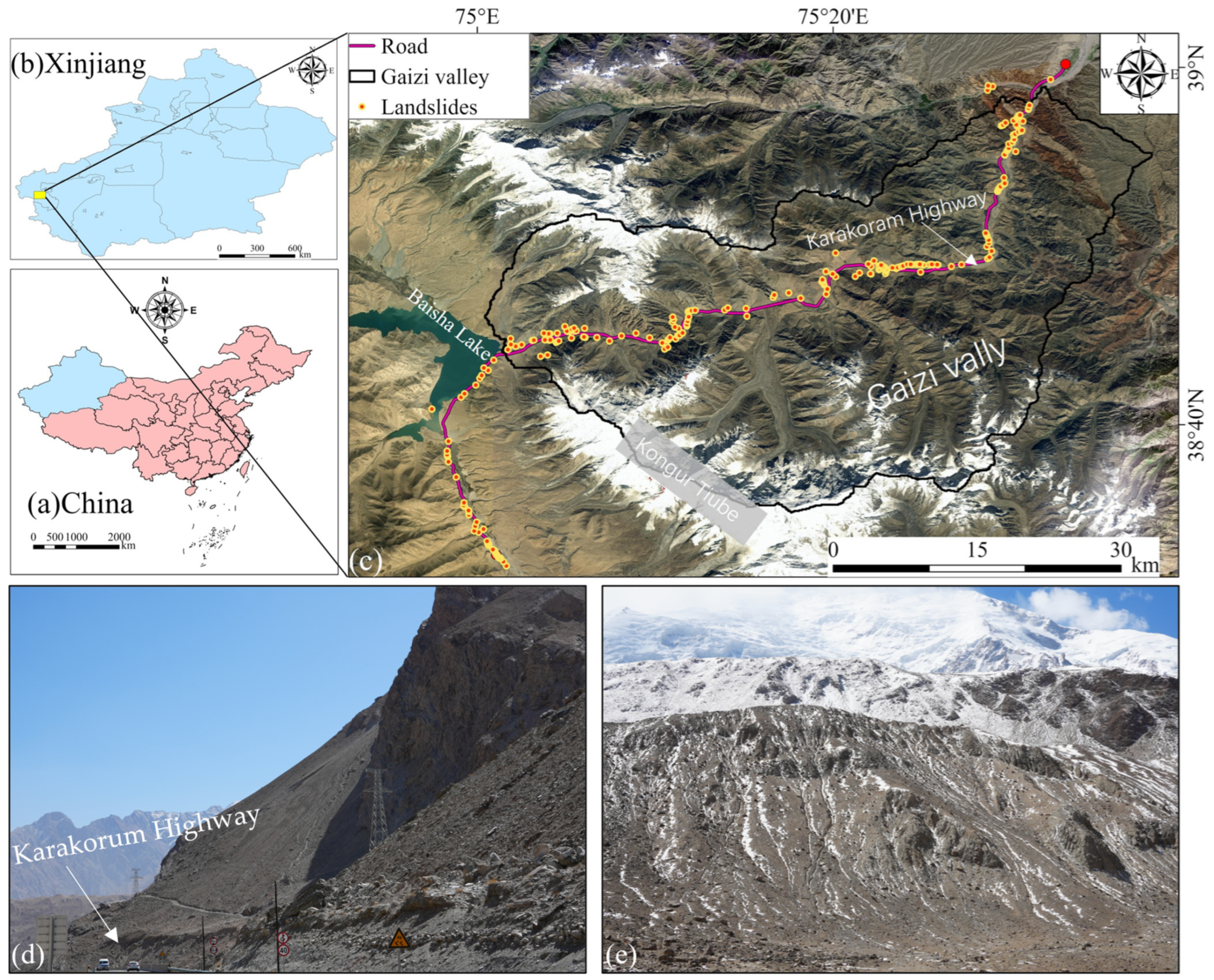
2.1. Research Area

The Karakoram Highway is a major transportation route from China to South Asia and the Middle East through Pakistan, starting from Kashgar in Xinjiang, China, in the north and ending in the northern town of Takot in Pakistan in the south, and was fully opened to traffic in 1979. The total length of the highway is 1224 km, including 415 km in China and 809 km in Pakistan. The highway passes through the mountainous areas where geological hazards are varied and concentrated [31]. The Gaizi River section is one of the most impacted sections of the entire highway, with a total of 276 landslides occurring from 1970 to 2020. This highway section, located on the northeastern edge of the Pamir Plateau, has a total length of approximately 94 kilometers, and the elevation gradually increases from east to west, with an average elevation of approximately 2970 m [32] (Figure 1). In the context of regional tectonics, the Gaizi Valley is characterized by extremely complex geological formations and combinations of magmatic rocks of different ages and lithologies. The region is characterized by a wide distribution of brown calcareous and cold calcareous soils, as well as saline irrigated soils, saline stony soils, calcareous meadow soils and frozen soils. The Gaizi Valley is located in the Eurasian hinterland; the climate is dry, and horizontal and vertical zonation is obvious. The average annual precipitation in the region is approximately 51 mm, and the average temperature is −1.5 °C. Under the effects of water-driven soil erosion and strong weathering, the regional ecological environment is fragile, the stability of slopes is poor, and the conditions are favorable for the occurrence of geological disasters such as landslides and collapses under the influence of earthquakes, rainfall, snow and ice meltwater and other factors. Due to the steepness of the hills and the looseness of the soils in the Gezi Valley area, the potential scope of impacts in the event of a landslide would be large. Therefore, after field surveys of the study area, this study will identify potential landslides within 3 km of the highway.

2.2. Materials

2.2.1. Historical Landslide Datasets

In this study, a dataset of the spatial distribution and attributes of typical failures and landslides in the China-Pakistan Economic Corridor (CPEC) from 1970 to 2020 was used for training the susceptibility model, and the data were obtained from the Institute of Geology and Geophysics, Chinese Academy of Sciences [33]. The collection of this landslide hazard dataset focuses on the major engineering facilities within CPEC. The dataset was based on Google Earth remote sensing imagery with a 10 m resolution, and the disaster sites were obtained through onsite investigations and remote sensing interpretation. The interpretation of landslide hazards compares multi-period remote sensing images, and the identification of disaster sites takes into account the structure of the disaster form, the degree of influence of the surrounding engineering facilities, the growth of vegetation and other factors. In addition, members of the research team have traveled to Kashgar, Xinjiang and other areas to conduct on-site surveys of landslides and slides for major projects in CPEC, such as KKH, in order to further supplement and validate the disaster data obtained from indoor remote sensing interpretation. Therefore, this landslide inventory dataset has a high level of confidence. Data were extracted from 276 landslide disaster points in the Gaizi Valley section of the Karakorum Highway, and the distribution of the disaster points is shown in Figure 1c. The historical landslide dataset was divided into a training set (70%) and a test set (30%) and applied in the landslide susceptibility analysis, which is presented in the subsequent methods section.

2.2.2. Selection of Indicators for Landslide Susceptibility Assessment

The selection of landslide-producing environmental factors is crucial to the construction of landslide susceptibility assessment systems and methods. In addition to the environmental factors that are closely related to landslides, such as precipitation, slope gradient, and slope direction [34,35], environmental factors such as snowmelt and proximity to a river channel were selected in this study with reference to previous studies and in combination with the geographic background conditions of the study area [31,32,36]. The selected factors can be categorized into four types [37]. The first type includes topographic factors, which include elevation, curvature, slope, aspect, the topographic position index (TPI), the terrain roughness index (TRI), and the topographic wetness index (TWI). The second category includes land cover factors, i.e., soil type and land cover type. The third category includes hydrologic elements, such as the modified normalized difference water index (MNDWI), river distance, and snowmelt. Finally, the fourth category includes engineering geology factors, such as the normalized difference built-up index (NDBI), fault distance, and epicenter distance. The weak correlation between the input data of the machine learning model needs to be satisfied [38]. Therefore, the correlations among the above preselected feature factors were calculated, and the factors with strong correlations (absolute values greater than 0.8) were excluded. The correlation results are shown in Figure 2. The correlation coefficient between the curvature and TPI is as high as 0.97, and the correlation coefficient between the slope and TRI is 0.96; these two pairs of factors are highly correlated, and the evaluation metrics obtained by removing one factor are shown in Figure 2b. The factor distributions are shown in Figure 3.

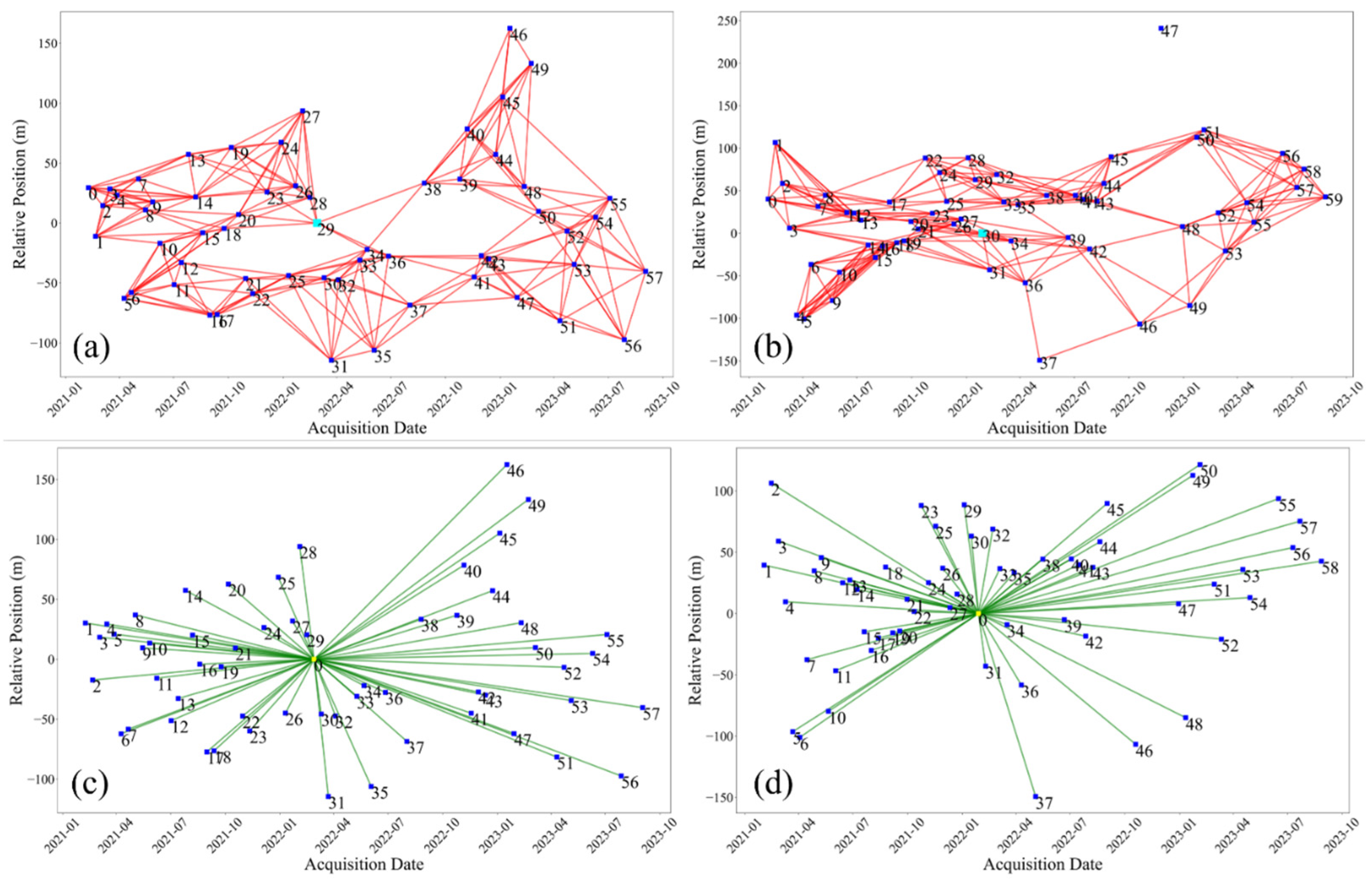
2.2.3. SAR Data and Interference Pair Information

Single look complex (SLC) data from Sentinel-1A of the 58-view ascending orbit and 60-view descending orbit were used to extract surface deformation from two radar lines of sight (LOS) of the ascending and descending orbits over the Gaizi Valley section of the Karakorum Highway. The acquired surface deformation time coverage is from 2 February 2021 to 2 September 2023, with an average of one view per half month for each single orbit, which can be increased to one observation of the region per week with a combination of both orbits. The data used are shown in

Table 1. Sentinel-1 image parameters.

Orbit	Image Coverage Time	Number of Images	Acquisition Mode	Polarization	Average Incidence Angle
Ascending	2021020—20230902	58	IW	VV	41.03
Descending	2021020—20230827	60	IW	VV	35.47

below.

The 30-meter DEM data from AW3D30 were used for terrain phase removal during interferometry of the Sentinel data, and POD precise orbit ephemerides were used for orbital phase error correction. In addition, Generic Atmospheric Correction Online Service (GACOS) data use the iterative tropospheric decomposition (ITD) model to separate the stratification and turbulence signals from the total tropospheric delay and to generate a high spatial resolution map of the total zenithal delay; this strategy was applied in this study to attenuate atmospheric phase delay effects [39,40,41].

This study used SBAS-InSAR and DS-InSAR to process the ascending and descending orbit Sentinel data, setting the maximum temporal baseline to 180 days, with the 58 Sentinel images of the SBAS-InSAR ascending orbit connected to form 234 interferometric pairs and the 60 Sentinel images of the descending orbit connected to form 235 interferometric pairs. The Sentinel image taken on 24 November 2022 was not included because it is beyond the threshold range of the spatial baseline (No. 47). The 58 Sentinel images of the DS-InSAR ascending orbit were connected to form 57 interference pairs, and the 60 Sentinel images of the descending orbit were connected to form 58 interference pairs. Figure 4 shows the interferometric image pair connections for the ascending and descending orbits. Overall, the spatial baseline of the Sentinel-1 data is small because of the strict orbit control.

2.3. Methods

2.3.1. Technical Process

The overall framework of the study is shown in Figure 5. The deformation map of the study area for 2021–2023 was obtained using time-series InSAR data, and the unstable slopes were identified in combination with optical images (Figure 5a). Second, we carried out the landslide susceptibility assessment, which included the construction of landslide susceptibility evaluation indices, the training of the machine learning model, and the validation of the model accuracy, to obtain the landslide susceptibility map of the area. Finally, the potential landslides were identified on the basis of deformation results and landslide susceptibility results.

2.3.2. Landslide Susceptibility Assessment Methodology

As the study area has received less attention, there is little previous research on landslide susceptibility in the region. Therefore, some qualitative or semi-quantitative landslide susceptibility methods based on experts’ experience, such as the analytic hierarchy process (AHP) [42,43], are largely inapplicable in the region. Quantitative methods, such as bivariate and multivariate logistic regression (LR), frequency ratios, and artificial neural networks (ANNs), focus on examining the influence of disaster-causing factors on the formation of geohazards and are therefore superior to qualitative methods in analyzing the risk of geohazards [44]. Among them, the main advantage of LR is its ability to handle various types of data, i.e., continuous, discrete, or combined, while ANNs have the advantages of a high modeling efficiency, simple application, and high stability [44,45]. Therefore, this study used two machine learning models, an artificial neural network and logistic regression, to evaluate the landslide susceptibility of the study area.

LR is a generalized linear regression model that predicts the probability of occurrence of landslide events in unknown samples via training with known sample landslide data. This technique characterizes landslide events as a binary categorical dependent variable and achieves nonlinear mapping between landslide events and influencing factors by establishing a binary relationship between landslides and non-landslides from 1 to 0, with which it predicts the probability of occurrence of a landslide event in any evaluation unit [46]. The landslide sensitivity predicted by the LR equation can be expressed as

$$x={\displaystyle \frac{e^{a_0+a_1{x}_1+a_2{x}_2+\cdots +a_n{x}_n}}{1+e^{a_0+a_1{x}_1+a_2{x}_2+\cdots +a_n{x}_n}}}$$

(1)

where y is the probability of landslide occurrence; x_i (i = 1, 2,…, n) are environmental factors; a_i is the contribution of each factor to the landslide occurrence; and a₀ is the regression intercept.

ANNs are similar to the self-organized structure of the biological nervous system of the mammalian brain, and their development and application overcome the problems faced by traditional statistical methods. These models can solve the problems of classification and regression and have been applied to the study of landslide susceptibility evaluation [47].

The list of landslides occurring in the region from 1970 to 2020 was randomly split into a training set (70%) and a test set (30%). Finally, the ROC curves obtained from the two models were plotted, and the AUC values were calculated. A highly accurate landslide susceptibility model was selected through comparative analysis, and the susceptibility mapping steps are shown in Figure 5b.

2.3.3. TS-InSAR Technology

When processing SAR images, the trade-off between the multi-look factor, filter window size and landslide detection capability should be fully considered. In this study, Sentinel-1 SAR images were processed using a multi-look factor of distance 4 (i.e., ground direction resolution of approximately 17 m) and azimuth 1 (i.e., resolution of approximately 14 m). After interfering with SAR images that satisfy the spatial and temporal baselines, filtering is performed using a localized stripe-based adaptive filtering function [48]. For the two time-series InSAR methods, this paper investigates the terrain phase removal aspect using 30 m DEM data from AW3D30 for simulation, POD data for orbit refinement correction to remove the orbital phase, and GACOS data to reduce the effect of atmospheric phase delays, thus obtaining a higher accuracy of the surface deformation phase. Finally, the phase is expanded using the minimum cost flow (MCF) [49] algorithm, and the annual average rate map is obtained after geocoding.

• SBAS-InSAR Principle

Assuming the possession of N + 1 views of SAR imagery covering the study area, M de-entangled interferograms are generated over a range that satisfies the spatiotemporal baseline. Points with higher coherence are considered high coherence points. The decoherence phase (corresponding to two moments t₁ and t₂) of the high coherence point (x,r) of the ith decoherence interferogram can be expressed as follows:

$$∆{\phi }_i(x,r)={\phi }_{t_2}(x,r)-{\phi }_{t_1}(x,r)\approx {\displaystyle \frac{4\pi }{\lambda }}(d(t_2,x,r)-d(t_1,x,r))+∆{\phi }_{top}^i+∆{\phi }_{noise}^i$$

(2)

where $d(t_1,x,r)$ and $d(t_2,x,r)$ represent the cumulative displacements in the radar LOS direction over the period t₁ to t₂; $∆{\phi }_{top}^i$ represents the uncertainty in the DEM due to the elevation residual phase; and the atmospheric phase, detangling errors, and other noise phases are usually denoted as $∆{\phi }_{noise}^i$. After the residual elevation phase is removed and the noise phase is suppressed with GACOS water vapor data, precision orbit data, and filtering methods, the phase is solved to solve the velocity term. The parameters to be solved are as follows:

$$v^T=\left[v_1={\displaystyle \frac{{\mathrm{\varnothing }}_1-{\mathrm{\varnothing }}_0}{t_1-t_0}},\dots ,v_N={\displaystyle \frac{{\mathrm{\varnothing }}_N-{\mathrm{\varnothing }}_{N-1}}{t_N-t_{N-1}}}\right]$$

(3)

The phases of all the interferograms are expressed in the above form. The combined expression is expressed in the error equation as follows:

$$\sum _{t_{1,i}+1}^{t_2,i}\left(t_k-t_{k-1}\right)V_k=∆{\phi }_i$$

(4)

The phases of all the interferograms are expressed in the above form. The combined expression is expressed in the error equation as follows:

$$AV=∆\phi$$

(5)

where A is a matrix with dimensions M × N. If a single interferogram subset is formed, the least squares method can be used to solve for the deformation rate. When two or more subsets of interferograms are created, a singular value decomposition (SVD) method with a least-paradigm condition needs to be introduced to obtain the deformation rate.

• DS-InSAR Principle

The DS-InSAR technique can be used to obtain a more complete deformation field by simultaneously detecting both distributed targets (DS) and permanent scatterer targets (PS) within range. The processing steps of the DS-InSAR technique used in the study are as follows:

(1)

Homogeneous image recognition. The study used an amplitude-based t-hypothesis approach to identify statistically homogeneous pixels (SHPs) [50]. Pixels with more connected SHPs than a threshold value of 20 can be regarded as distributed target candidates (DSCs) in the subsequent phase optimization operation [51,52]. The original hypothesis and alternative hypotheses of the two-sample t-hypothesis test are as follows:

$$H_0:{\mu }_1={\mu }_2,H_1:{\mu }_1\ne {\mu }_2$$

(6)

where ${\mu }_1$ and ${\mu }_2$ are the mean values of the SAR image amplitudes in the two samples, and the test statistics of the samples are expressed as follows:

$$t={\displaystyle \frac{\overline{A}\left(P_1\right)-\overline{A}\left(P_2\right)}{\sqrt{\frac{{\sigma }^2\left(P_1\right)+{\sigma }^2\left(P_2\right)}{N}}}}$$

(7)

where t is the test statistic of the sample, which obeys the t-distribution; $P_1$ and $P_2$ are the two image elements to be tested; $\overline{A}\left(P\right)$ is the mean value of the sample amplitude of the image element; ${\sigma }^2\left(P_1\right)$ and ${\sigma }^2\left(P_2\right)$ are the sample amplitude variances of the image elements $P_1$ and $P_2$; and N denotes the sample capacity.

(2)

Phase optimization. Assuming that n is the number of SAR images and l is the number of homogeneous pixels, the complex coherence matrix can be calculated via Equation (8).

$$T={\displaystyle \frac{Z{Z}^H}{\sqrt{{\Vert Z\Vert }^2{\left({\Vert Z\Vert }^2\right)}^T}}}$$

(8)

where $\Vert \Vert$ is the paradigm operation performed on the matrix rows, T is the sample complex coherence matrix, Z is the n × l homogeneous image matrix, and ${\left({\Vert Z\Vert }^2\right)}^T$ is its transpose matrix. In this study, phase optimization is achieved via an interferometric phase maximum likelihood estimation (EMI) [53] method that is based on feature decomposition. The computational formula is as follows:

$$\widehat{\sum }={argmax}_{\sum }\left\{\mathrm{l}\mathrm{n}\left(p\left(T|\sum \right)\right)\right\}={argmin}_{\varphi ,\sigma ,\alpha }\left\{{\alpha }^{-2}{\zeta }^H\left({\mathsf{\Gamma }}^{-1}\circ {\rm T}\right)\zeta -\sum _{i=1}^n\mathrm{l}\mathrm{n}\left({\left(\alpha {\sigma }_i\right)}^{-2}\right)\right\}$$

(9)

where Г is the coherence matrix, $\varphi$ is the optimized phase, $\zeta$ is the reciprocal of the optimized phase, and $\sigma$ and $\alpha$ are scale parameters that provide additional degrees of freedom for the calibration of Г. Linearizing $\mathrm{l}\mathrm{n}\left({\left(\alpha {\sigma }_i\right)}^{-2}\right)$ in Equation (9) with a Taylor series and adding a paradigm constraint on $\sigma$ via Lagrange multipliers, the equation to be solved is thus transformed to

$$\left({\mathsf{\Gamma }}^{-1}\circ {\rm T}\right)\widehat{\zeta }=\lambda \widehat{\zeta }$$

(10)

Equation (10) can be used to find the eigenvector corresponding to the smallest eigenvalue via eigen decomposition, and the phase of the original image element can be replaced with the phase of the eigenvector to achieve phase optimization. After the DS and PS targets are selected and fused by setting the threshold value of the temporal coherence coefficient, phase untangling and error correction, such as atmospheric delay, are completed according to the basic flow of temporal InSAR data processing, and finally, the deformation information of the study area is obtained.

2.3.4. Potential Landslide Identification and Analysis

The identification of potential landslides was carried out in the following steps. First, on the basis of the results of landslide susceptibility analysis, the distance of unstable slopes from the high-incidence area is used as the basis of discrimination, and the results of InSAR identification are screened and rejected. Second, a comprehensive analysis of the regional geology, topography, and soil type is performed to assist in the identification of potential landslides. Finally, on the basis of the results of the identification of potential landslides, a field investigation is carried out to verify the results.

3. Results

3.1. Deformation Results

Figure 6 shows the results for the annual average deformation rate of the Gaizi Valley section of the Karakorum Highway for the years 2021–2023. In Figure 6, (A) and (B) are the ascending- and descending-orbit SBAS-InSAR results, respectively, and (C) and (D) are the ascending- and descending-orbit DS-InSAR results, respectively. The region generally experienced uplift, and the ascending- and descending-orbit results all show positive mean annual deformation rates (Figure 7). The maximum surface subsidence (LOS direction) rate obtained from ascending-orbit SBAS-InSAR data is −58.64 mm/year, the maximum surface subsidence rate obtained from the ascending-orbit DS-InSAR data is −62.85 mm/year, the maximum surface subsidence rate obtained from descending-orbit SBAS-InSAR data is −45.08 mm/year, and the maximum surface subsidence rate obtained from the descending-orbit DS-InSAR data is −45.17 mm/year, as shown in Figure 7. The surface subsidence rate is −45.17 mm/year, as shown in Figure 7. The difference between the maximum surface subsidence rates obtained in the same orbit direction is small, and both methods reveal that the maximum subsidence rate detected in the ascending orbit direction is slightly greater than that detected in the descending orbit direction, which may be caused by the different geometric relationships between the radar angle of incidence and the mountain slopes. However, for both ascending and descending orbits, the surface deformation results obtained via the two time-series InSAR methods have a high degree of consistency in terms of spatial distribution and deformation magnitude (Figure 6 and Figure 7), and overall, the number of monitoring points obtained via DS-InSAR is larger than that obtained via SBAS-InSAR.

A landslide is defined as a physical system that develops in stages over time, including pre-damage deformation, the damage-causing event itself, and subsequent yield displacement [54]. According to previous studies, for C-band datasets, deformation rates greater than 2 mm/year in the LOS direction can be considered indicators of unstable slopes [55]. However, owing to the strong regional tectonics and the accompanying ice and snow meltwater erosion of the geotechnical bodies in this study area, deformation zones with average annual rates greater than −20 mm/year were classified as unstable slopes (within the white boundary in Figure 6). In total, 44 unstable slopes were detected in the ascending orbit direction of SBAS-InSAR, and these slopes were classified into seven unstable slope clusters (black box in Figure 6). Additionally, unstable slopes were detected in the descending orbit direction, with a total of six unstable slope clusters. A total of 73 unstable slopes were detected in the ascending orbit direction of DS-InSAR, with eight unstable slope clusters, and 77 unstable slopes were detected in the descending orbit direction, with seven unstable slope clusters. A total of 116 unstable slopes were detected in the ascending- and descending-orbit datasets, with 80 unstable slopes detected in the ascending-orbit datasets and 90 detected in the descending-orbit datasets. Most of the unstable slope complexes are distributed on mountains within 3 km of the Gaizi Valley (Figure 6), and the other three concentrations are distributed on the northwestern foothills of Kongur Tiube, at the exit of the Gaizi Valley, and on the mountains southwest of Baisha lake.

However, the unstable slopes identified with time-series InSAR data only indicate that the area had a high degree of deformation within the monitoring time range and cannot be judged as potential landslide areas. Therefore, it is necessary to further analyze each unstable slope to determine the probability and risk of producing a landslide disaster and to identify the areas that have severe settlement and a high probability of producing a landslide disaster.

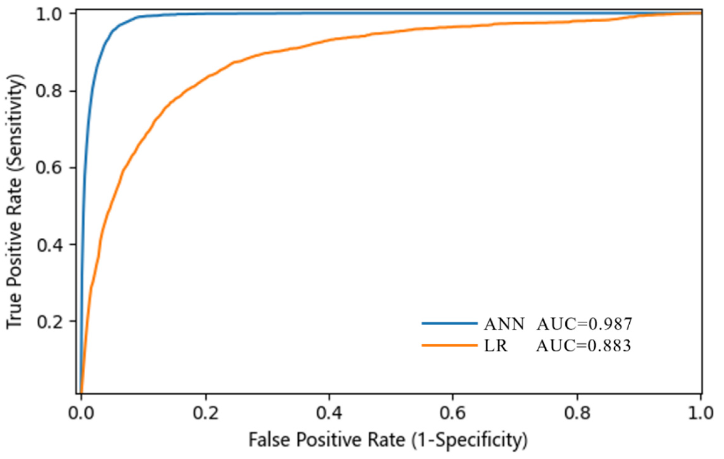
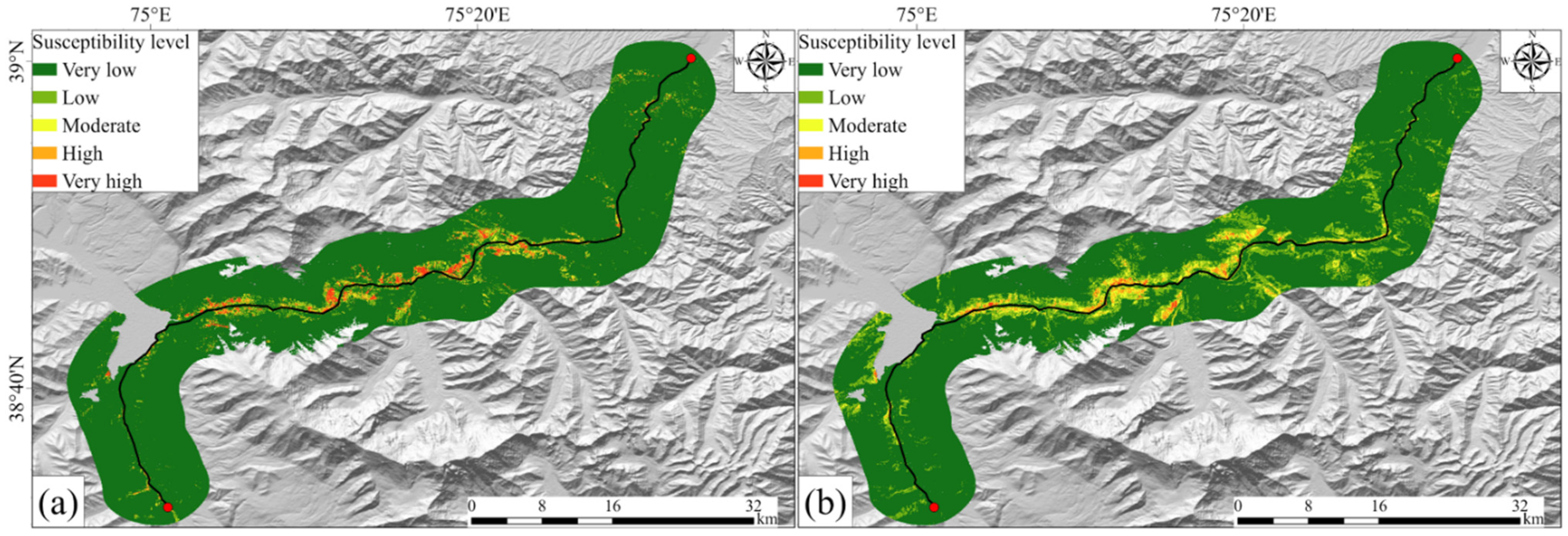
3.2. Landslide Susceptibility Results

In this study, the problem is treated as a binary classification task that classifies a sample into landslide (positive) and non-landslide (negative) categories. The probability of a sample being positive is taken as its susceptibility, ranging from 0 to 1. The classification accuracy of a model is given by

Accuracy = (TP + TN)/(TP + FP + TN + FN)

(11)

where TP represents true positive predictions, which means the prediction and sample true category are both positive; FP represents the false positive predictions, indicating that the prediction is positive but the sample is indeed a negative one; TN are true negative predictions and FN are false negative predictions. The F1 score is another widely used accuracy indicator [11], obtained from precision (given by TP/(TP + FP)) and recall (given by TP/(TP + FN)), and is calculated as shown in Equation (12). See

Table 2. Comparison of performances of two artificial intelligence algorithms trained with landslide data from 1970 to 2020.

Artificial Intelligence Algorithms	Accuracy	Precision	Recall	F1 Score	Area Under Curve
LR	0.801	0.868	0.711	0.768	0.883
ANN	0.916	0.936	0.892	0.934	0.987

for detailed model performance.

$${\mathrm{F}}_1\mathrm{s}\mathrm{c}\mathrm{o}\mathrm{r}\mathrm{e}={\displaystyle \frac{2}{\frac{1}{\mathrm{P}\mathrm{r}\mathrm{e}\mathrm{c}\mathrm{i}\mathrm{s}\mathrm{i}\mathrm{o}\mathrm{n}}+\frac{1}{\mathrm{R}\mathrm{e}\mathrm{c}\mathrm{a}\mathrm{l}\mathrm{l}}}}$$

(12)

The ROC curves of the landslide susceptibility results from the two models were compared, and the corresponding area under the curve (AUC) of the two models was calculated. When the AUC value is closer to 1, the model assessment accuracy is better [56]. As shown in Figure 8, the ANN model, with an AUC value of 0.987, is more accurate than the LR model, with an AUC value of 0.883.

The natural breakpoint method was subsequently applied to classify the susceptibility, i.e., a total of five levels, namely, very low hazard, low hazard, moderate hazard, high hazard and extremely high hazard [57]. The graded landslide susceptibility results are shown in Figure 9. The medium and high landslide susceptibility areas of the Gaizi Valley section of the KKH in the two models were determined. The area of medium- and high-hazard areas in the ANN model was 3.63 km², accounting for 4.55% of the total area of the study area. The area of medium- and high-hazard areas derived from the LR model was 4.19 km², accounting for 5.25% of the total area of the study area. The specific area of each hazard level and the proportion of area of each level are shown in

Table 3. Areas and percentages of the landslide hazard classes.

Model	Very Low		Low		Moderate		High		Very High
	Area (km2)	Percentage (%)	Area (km2)	Percentage (%)	Area (km2)	Percentage (%)	Area (km2)	Percentage (%)	Area (km2)	Percentage (%)
ANN	73.25	91.78	2.92	3.67	1.46	1.83	1	1.26	1.16	1.46
LR	65.95	82.62	9.68	12.13	2.78	3.48	1.23	1.54	0.19	0.23

. Then, to determine whether the landslide susceptibility results obtained from the LR and ANN models are significant or not, t tests are conducted for these two models. The t test results show that the t value is 8.75, which is greater than the critical value of 1.95, and the p value is much less than 0.05, i.e., there is a significant difference in the landslide susceptibility results obtained from the ANN and LR models. Although the LR model took less time than the ANN model, the classification accuracy of the ANN model was higher than that of the LR model, so the landslide susceptibility results from the ANN model were used in the subsequent analysis.

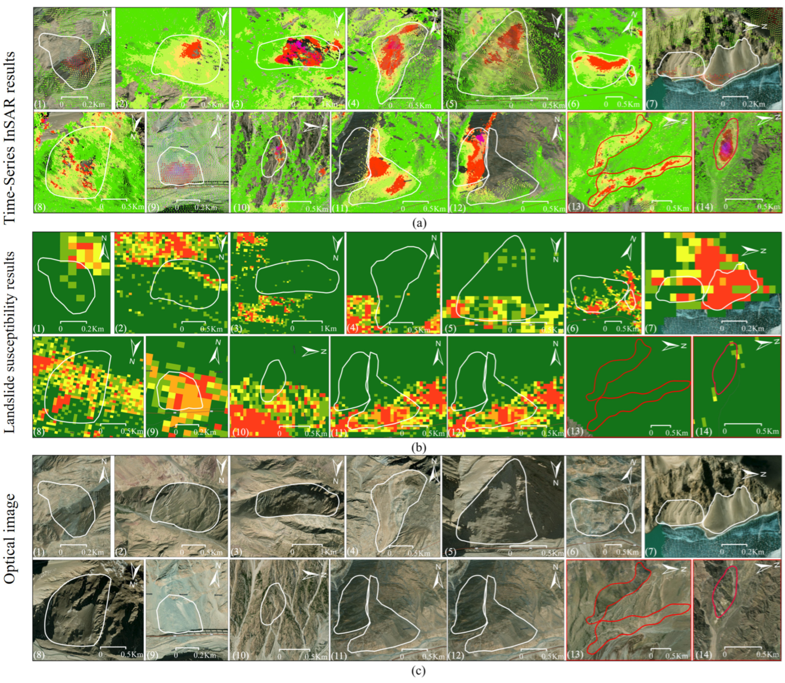
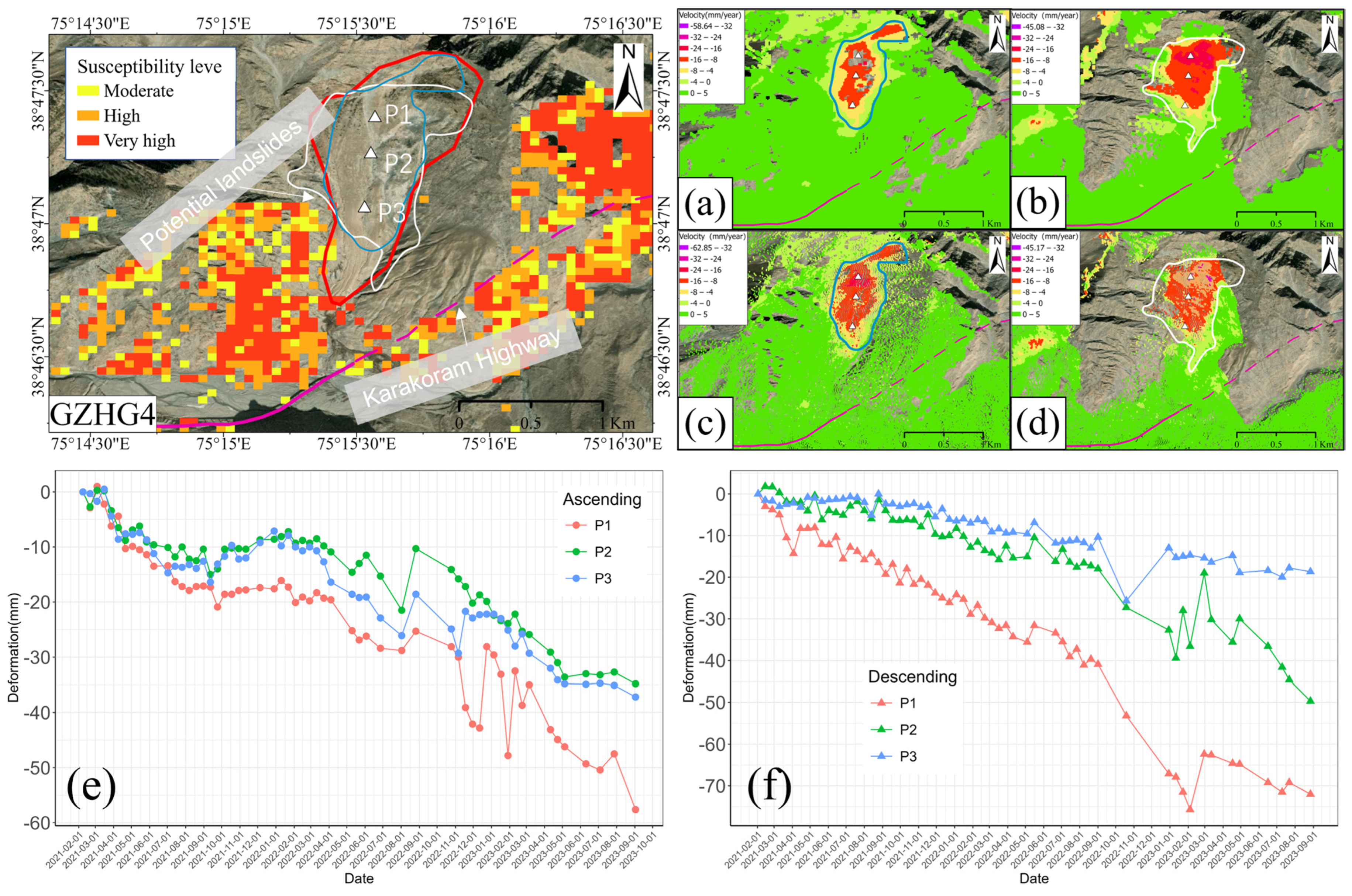
3.3. Potential Landslide Identification

On the basis of the results of time-series InSAR deformation and landslide susceptibility analysis from 2021 to 2023, potential landslides are further identified by combining high-resolution images and field surveys, and their vector boundary ranges are plotted according to the regional deformation and geological texture of slopes. A total of 14 potential landslides were identified in the region, and their distribution locations are shown in Figure 10. Specific information on potential landslides is shown in

Table 4. Information on potential landslides.

Number	Longitude	Latitude	Area (km2)	Aspect	Slope (°)	Elevation Difference (m)
GZHG1	75.46	38.87	0.16	NE	41.31	326
GZHG2	75.31	38.81	3.27	NE	35.96	1144
GZHG3	75.34	38.83	1.57	NE	32.43	714
GZHG4	75.26	38.79	1.44	S	34.71	1139
GZHG5	75.25	38.77	1.05	NE	35.83	903
GZHG6	75.22	38.76	1.86	NE	35.59	1105
GZHG7	75.21	38.77	0.13	SE	34.37	235
GZHG8	75.18	38.77	0.25	E	37	280
GZHG9	75.07	38.75	1.11	SE	40.73	1060
GZHG10	75.07	38.76	0.71	SW	38.09	828
GZHG11	75.06	38.75	0.16	SE	43.71	335
GZHG12	75.05	38.75	1.96	SE	34.88	768
BSH1	74.96	38.68	0.08	E	32.95	71
BSH2	74.96	38.68	0.12	NE	45.69	239

. The number of unstable slopes with potential landslides is shown in Table 4.

In total, 12 potential landslides were identified in the Gaizi River valley section, and two potential landslides were identified in the Baisha Lake section at the exit of the Gaizi River valley. The potential landslides in the Gaizi River valley section are distributed on slopes on both sides of the highway, and the nearest potential landslide (GZHG7) is less than 50 m from the highway, which threatens the normal operation of transportation in the event of a landslide or rockfall. Figure 11a–c show high-resolution images of 14 potential landslides and the results for the annual mean deformation rate in the Gaizi River section of the Karakorum Highway.

Table 5. Number of unstable slopes and potential landslides.

Orbit	Methods	Number of Unstable Slopes	Number of Common Unstable Slopes	All Unstable Slopes	Potential Landslides
Ascending	SBAS-InSAR	44	37	116	14
	DS-InSAR	73
Descending	SBAS-InSAR	57	44
	DS-InSAR	77

shows the number of unstable slopes detected by the two TS-InSAR methods in both directions. In general, the deformation rates and distribution areas derived from the DS-InSAR and SBAS-InSAR data are in good agreement, suggesting these datasets can be used to identify potential landslides.

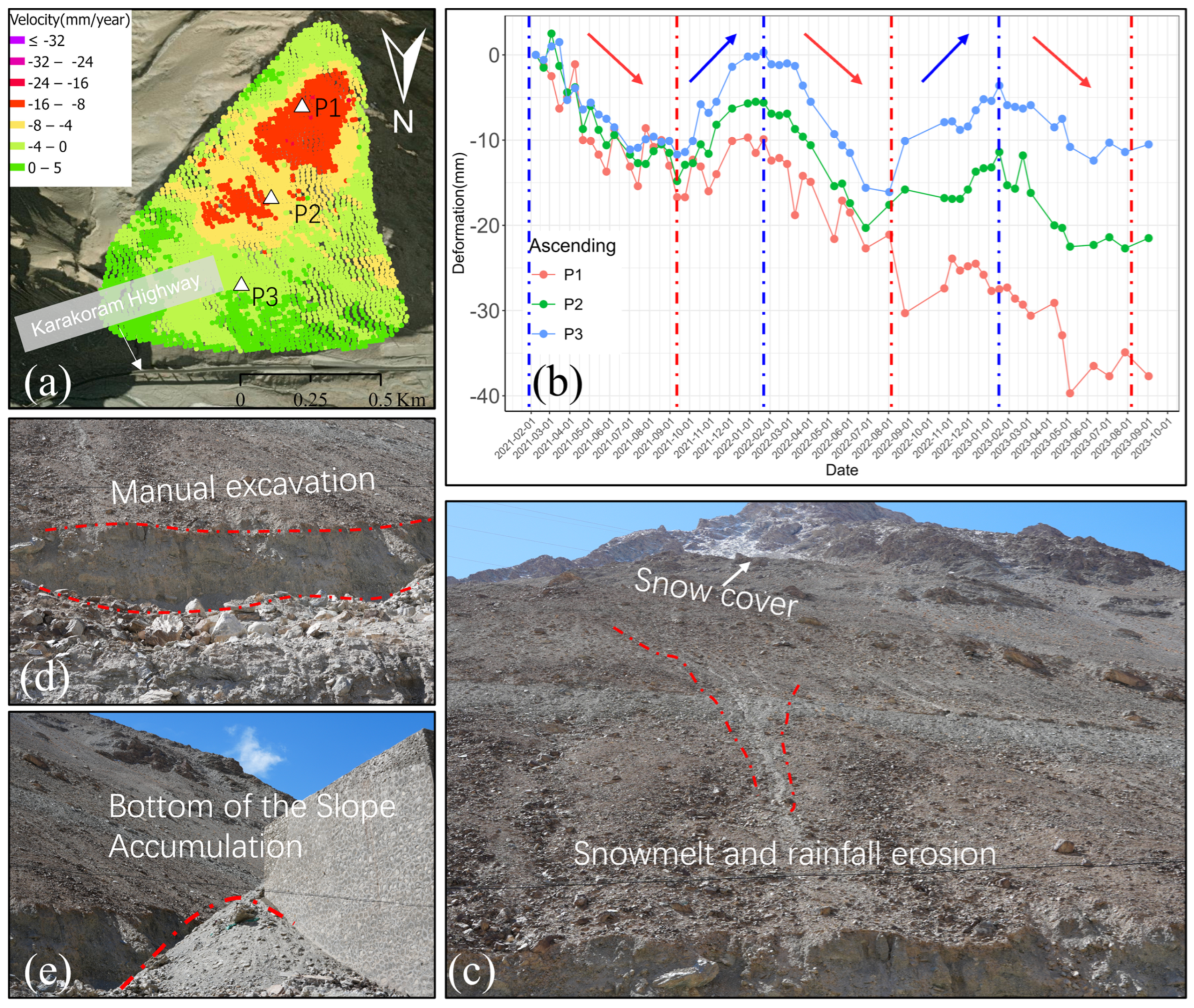
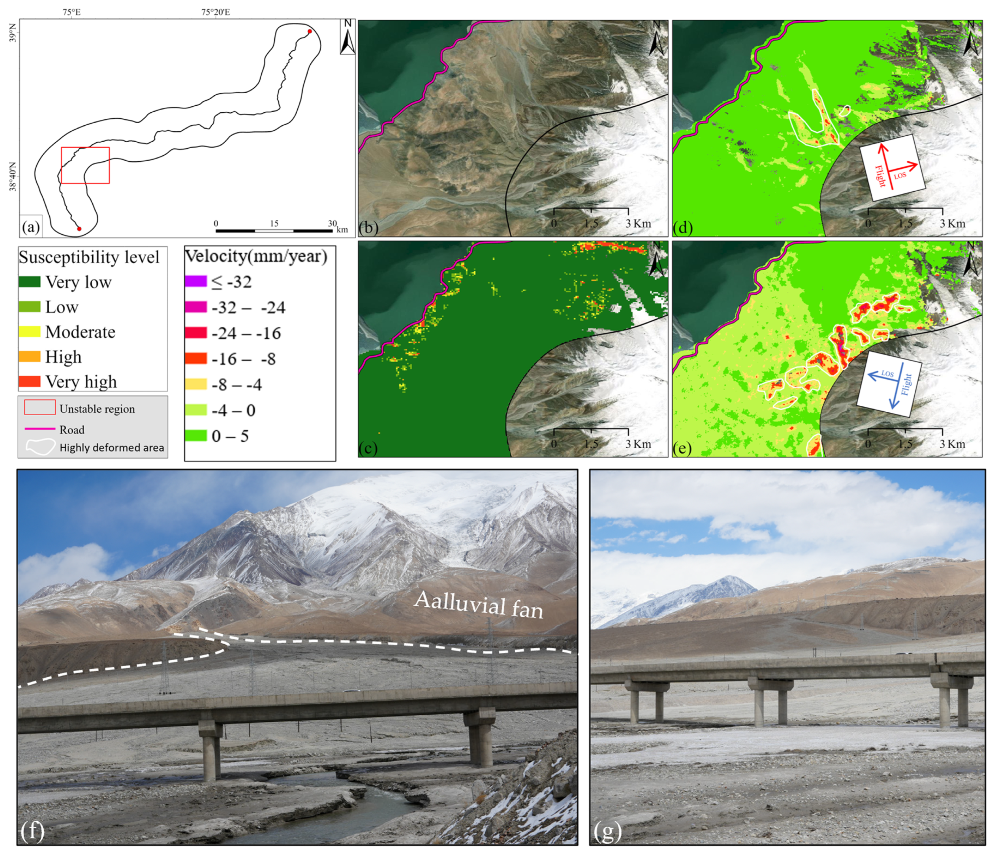
3.4. Potential Landslide Analysis and Validation

A total of 14 potential landslides and their characteristics were identified in the study, and the potential landslides that are close to and threaten the Karakorum Highway are discussed in detail below. Furthermore, their spatiotemporal deformation characteristics are analyzed.

The slope body located above the tunnel entrance of the Gaizi Valley section of the Karakorum Highway, with a longitude of 75°15′30″ and a latitude of 38°47′15″, is labeled GZHG4, as shown in Figure 12. The slope body faces approximately southwest and has a gradient of 20–43°. The foot of the slope is relatively gentle, and the top of the slope has a relatively high gradient. The unstable slope is approximately 600 m wide and 800 m long. The area with a high rate of deformation in Figure 12a–d is circled with a blue circle and a white circle, and it is judged to be an unstable slope. The red-circled portion is a potential landslide derived from the susceptibility map with high-resolution imagery and field survey data. Although the unstable slopes identified with the time-series InSAR data do not completely overlap with the high-hazard susceptibility area, they are very close to the high-hazard section (<100 m); thus, the slopes have the potential for landslides. The reason for the biased results may be related to the accuracy of the historical landslide dataset. The extent of landslides in the historical landslide dataset is more focused on the accumulation zone, whereas the time-series InSAR data reflect deformation in the source zone above the slope. Since SBAS-InSAR and DS-InSAR have high agreement in terms of deformation magnitude and deformation distribution, the temporal deformation rate derived from the DS-InSAR data was selected for analysis. To explore the deformation characteristics of the slope body, we selected three points from the slope body for temporal analysis, namely, points P1, P2, and P3 from top to bottom. Figure 12e,f show that the three points along an elevation track can provide deformation estimates away from the LOS direction. Among the points, point P1, which is located in the upper part of the slope body, has the largest deformation, which is best observed in the LOS direction of the descending track, and downward sliding deformation accelerated between September 2022 and February 2023. Point P1 exhibits upward deformation in the LOS direction of the descending track, reaching −72 mm in the period from February 2021 to September 2023, and upward deformation in the LOS direction of the ascending track, reaching −57.6 mm. Overall, the deformation rate of the upper part of this slope is greater than that of the lower part of the slope. In landslide studies, heavy rainfall, earthquakes, water level changes, rapid snowmelt, volcanic eruptions, and human activities are the most common landslide triggers [14,58,59]. The optical images revealed that the slope had traces of water scouring and erosion during snowmelt or rainfall and was located above the tunnel; thus, engineering disturbances and water erosion could have caused the instability of the slope. Owing to its close proximity to the highway, high gradient and loose soil, measures should be implemented to prevent this slope from blocking the tunnel portal in the case of a landslide, which would pose a great threat to the normal operation of the highway.

GZHG5 is located on the south slope of the Karakorum Highway, with a gradient of approximately 35.8° toward the northeast, and the detailed information of GZHG5 is listed in Table 3. In the surface deformation distribution, the deformation rate of the upper part of the slope is larger than that of the lower part, as shown in Figure 13a, which is similar to GZHG4. Although the slope is in subsidence, unlike GZHG4, the deformation of GZHG5 exhibits cyclic variations, as shown in Figure 13b. Studies of snow cover in the Karakoram and Western Kunlun regions have shown that February and August are the highest and lowest snow cover months in the region [60]. Therefore, the reason for the cyclic deformation of the slope may be closely related to the melting of the snowpack, which takes place from February to August or September, while snowfall gradually starts in the region from September to February, and the melting of the snowpack has an impact on the stability of the slope. In addition, our field survey found many rocks tumbling down from the mountain at the foot of the slope (Figure 13d), as well as loose piles (Figure 13c), and the surface of the slope showed traces of erosion from snowmelt (Figure 13c). The field verification indicates that the slope is in an unstable condition, which further verifies that the potential landslides identified in this study are reliable.

4. Discussion

4.1. Strengths and Weaknesses of Dual-Orbit Time-Series InSAR Monitoring of Potential Landslides

Overall, the potential landslides identified by the two time-series InSAR datasets are in good agreement with the corresponding landslide geomorphic features, and the boundaries of the large deformation rates are also consistent with the boundaries of the slopes in the optical images, as shown in Figure 11a,c. It has been shown that a significant amount of decoherence occurs when applying Sentinel 1 data to more densely vegetated areas, thus reducing the coverage of landslide monitoring [61]. However, the vegetation in this study area is extremely sparse and is mostly bare soil and rock. Therefore, C-band Sentinel 1A data can be well applied to this study area, and if the method used in this study is applied to more densely vegetated areas, the use of L-band SAR data with longer wavelengths should be considered [24]. The study area is located in an alpine mountainous area with steep terrain, so single-orbit SAR data will inevitably produce geometric distortions such as superimposed masks (high-slope areas) and shadows (no radar signal echoes) [62] during side-view imaging, and geometric aberrations will lead to blind zones in single-orbit observations, resulting in omissions in landslide detection [63]. As shown in Figure 11(11), for the ascending-orbit deformation monitoring results, potential landslides in the region to the left of the figure (GZHG10) could not be detected in the ascending orbit direction because the ascending-orbit LOS direction has no echo signals in this region. The study was supplemented with descending-orbit data (Figure 11a(12)), and this region is significantly deformed in the descending-orbit LOS direction. This shows that the joint identification of potential landslides by descending and ascending orbits has spatial advantages, and the simultaneous detection of an area with descending- and ascending-orbit data results in a more complete distribution of surface deformation in the Gaizi Valley. However, owing to the steep terrain in some areas of the study area, the backscattered signals from slopes are not received in either direction of the elevation track, so potential landslides might be missed. The two time-series InSAR methods, SBAS-InSAR and DS-InSAR, can obtain deformation estimates for most of the study area (Figure 6), and there is consistency in the distribution and magnitude of the deformation. The annual deformation of the four results (including the elevation track) is consistent with the deformation distribution of the study area. The annual deformation rates, including those of the ascending orbits, differ within 1.5 mm (Figure 7). The standard deviation of the annual deformation rate of SBAS-InSAR is stable at 2.6–2.7 mm, whereas the standard deviation of DS-InSAR is in the range of 2.5–2.8 mm, and the annual mean deformation rate of the ground surface obtained by SBAS-InSAR is more stable than that of DS-InSAR. Finally, the phase difference information of SAR can be used to monitor only slow creeping landslides. Out-of-phase coherence occurs for some fast-moving slopes or landslides that have already occurred, such as (1) and (7) in Figure 11a, so the approach taken in the study has limitations in this regard. For areas with high deformation, the method of coherence coefficient difference or L-band satellite images can be considered for landslide detection and identification.

4.2. Natural Factors Interfere with Potential Landslide Identification

As shown in the red box in Figure 13a, large subsidence events (with subsidence rates greater than −32 mm/year) were detected in this area in both the ascending- and descending-orbit time-series InSAR datasets. The region is located at the exit of the Gaizi Valley section of the KKH, at the northwestern foot of Kongur Tiube, approximately 3 km from the highway. The area generally exhibits uplift, which is more pronounced in the direction of the LOS of the ascending track (Figure 14d). Subsidence zones were identified in both the ascending and descending tracks, as shown in the white circled portions of Figure 14d,e, and the subsidence zones were more pronounced in the descending-track LOS direction, with higher subsidence rates over a wider area. However, the results of the landslide susceptibility analysis reveal that this area is not a high-risk landslide area, as shown in Figure 14c, indicating that this area generally does not have the environmental conditions for landslides. Based on the high-resolution image in Figure 14b, the lower left part of the area is a giant alluvial fan, which is formed by snow melt and rainfall in the spring and summer seasons. When heavy rainfall, flash floods, or large amounts of snowmelt occur in alpine areas, water flows rapidly down slopes, carrying large amounts of sediment and debris. This strong water flow scours hillsides and mobilizes sediments at the bottom of the channel. When flood flow slows, the sediment and debris carried by the water begin to be deposited. As the velocity of the water decreases, less sediment is able to be carried and transported, and the sediment gradually accumulates on the foothill plains. From this, it can be preliminarily judged that the subsidence in this area is basically driven by water-induced erosion of the rocks and soil and that the area is not a site of potential landslides.

4.3. Identification of Potential Landslides Disturbed by Engineering Activities

In addition to some natural factors that can produce regional subsidence, anthropogenic factors may also lead to regional subsidence, thus affecting the judgment of potential landslides. As shown in Figure 15d, the subsidence area detected by the ascending SBAS-InSAR is located in the entrance section of the Gaizi River valley (red triangle in Figure 15a), which is approximately 1 km away from the Karakorum Highway, and the Gaizi River is on the right side of the highway. As shown in Figure 15d, the deformation rate of the subsidence center exceeds −32 mm/year, and incoherence is observed on the left side of the area. Without landslide susceptibility analysis, this area could be easily misclassified as a potential landslide body that has been partially dislodged, and most of the area in Figure 15c is in the low susceptibility and very low susceptibility zones. To further verify whether this area is a potential landslide area, we conducted a field survey and found that it is a mineral development area, as shown in Figure 15e. The field verification combined with the analysis of high-resolution imagery ultimately ruled out the presence of potential landslides in this area.

5. Conclusions

Located in an alpine mountainous area, the Gaizi Valley section of the Karakorum Highway is characterized by steep terrain and severe slope erosion, and landslide hazards are widely distributed and need to be identified and managed at an early stage. This study couples landslide susceptibility characteristics with regional deformation characteristics and proposes a new identification method for potential landslides in the Gaizi River Valley section of the Karakorum Highway, where the terrain is steep and the region itself has large deformation.

The joint orbital track analysis technique was used to monitor unstable slopes via two time-series InSAR datasets covering the period from February 2021 to September 2023 in the Gaizi Valley section of the Karakorum Highway. The results show that the joint orbital track time-series InSAR approach can be applied to steep mountainous terrain and can effectively identify unstable slopes and that the orbital track data yield spatially complementary results. A total of 116 unstable slopes were detected in the ascending- and descending-orbit datasets, of which 80 unstable slopes were detected in the ascending-orbit dataset and 90 in the descending-orbit dataset. The DS-InSAR and SBAS-InSAR monitoring results are in good agreement in terms of the distribution and magnitude of deformation, and the difference in the annual average deformation rate is ±0.5 mm, with a variance within an acceptable range. To understand the magnitude of the probability of landslide occurrence on each unstable slope and to identify potential landslides, landslide hazard analysis was performed via the regional historical landslide dataset for a total of 50 years from 1970 to 2020 in combination with 13 landslide susceptibility factors. The results show that most of the hazard-prone areas are located on both sides of the highway, and the classification accuracy of the ANN model is greater than that of the LR model. The area of medium–high hazard derived from the ANN model is 3.63 km², accounting for 4.55% of the total area of the study area, and the area of medium–high hazard derived from the LR model is 4.19 km², accounting for 5.25% of the total area of the study area. After deformation monitoring and susceptibility assessment, 14 potential landslides were identified on the basis of regional deformation characteristics, landslide susceptibility characteristics, high-resolution optical images, field surveys and other auxiliary means. These 14 potential landslides have the potential to form landslides with a high degree of risk, and they need to be mitigated and closely monitored in real time.

Overall, the combination of joint orbital track time-series InSAR deformation monitoring and landslide susceptibility mapping methods can yield a highly accurate list of potential landslides. However, there may be some omissions and misjudgments in the process, which depend on various factors. On the one hand, there are factors that interfere with InSAR data, such as atmospheric delays and geometric distortions, and on the other hand, there are errors in landslide susceptibility mapping, such as the lack of details in the landslide inventory and the selection of landslide environmental factors and landslide susceptibility models.

References

1. Tehrani, F.S.; Calvello, M.; Liu, Z.; Zhang, L.; Lacasse, S. Machine Learning and Landslide Studies: Recent Advances and Applications. Nat. Hazards 2022, 114, 1197–1245. [Google Scholar] [CrossRef]
2. Chae, B.-G.; Park, H.-J.; Catani, F.; Simoni, A.; Berti, M. Landslide Prediction, Monitoring and Early Warning: A Concise Review of State-of-the-Art. Geosci. J. 2017, 21, 1033–1070. [Google Scholar] [CrossRef]
3. Froude, M.J.; Petley, D.N. Global Fatal Landslide Occurrence from 2004 to 2016. Nat. Hazards Earth Syst. Sci. 2018, 18, 2161–2181. [Google Scholar] [CrossRef]
4. Dilley, M. Natural Disaster Hotspots: A Global Risk Analysis; Disaster Risk Management Series; World Bank: Washington, DC, USA, 2005; ISBN 978-0-8213-5930-3. [Google Scholar]
5. Sassa, K.; Canuti, P.; International Consortium on Landslides (Eds.) Landslides: Disaster Risk Reduction; Springer: Berlin/Heidelberg, Germany, 2009; ISBN 978-3-540-69966-8. [Google Scholar]
6. Thi Ngo, P.T.; Panahi, M.; Khosravi, K.; Ghorbanzadeh, O.; Kariminejad, N.; Cerda, A.; Lee, S. Evaluation of Deep Learning Algorithms for National Scale Landslide Susceptibility Mapping of Iran. Geosci. Front. 2021, 12, 505–519. [Google Scholar] [CrossRef]
7. Mantovani, J.R.; Bueno, G.T.; Alcântara, E.; Park, E.; Cunha, A.P.; Londe, L.; Massi, K.; Marengo, J.A. Novel Landslide Susceptibility Mapping Based on Multi-Criteria Decision-Making in Ouro Preto, Brazil. J. Geovis. Spat. Anal. 2023, 7, 7. [Google Scholar] [CrossRef]
8. Pradhan, B.; Dikshit, A.; Lee, S.; Kim, H. An Explainable AI (XAI) Model for Landslide Susceptibility Modeling. Appl. Soft Comput. 2023, 142, 110324. [Google Scholar] [CrossRef]
9. Dou, J.; Yunus, A.P.; Bui, D.T.; Merghadi, A.; Sahana, M.; Zhu, Z.; Chen, C.-W.; Han, Z.; Pham, B.T. Improved Landslide Assessment Using Support Vector Machine with Bagging, Boosting, and Stacking Ensemble Machine Learning Framework in a Mountainous Watershed, Japan. Landslides 2020, 17, 641–658. [Google Scholar] [CrossRef]
10. Wu, X.; Song, Y.; Chen, W.; Kang, G.; Qu, R.; Wang, Z.; Wang, J.; Lv, P.; Chen, H. Analysis of Geological Hazard Susceptibility of Landslides in Muli County Based on Random Forest Algorithm. Sustainability 2023, 15, 4328. [Google Scholar] [CrossRef]
11. Wang, H.; Zhang, L.; Luo, H.; He, J.; Cheung, R.W.M. AI-Powered Landslide Susceptibility Assessment in Hong Kong. Eng. Geol. 2021, 288, 106103. [Google Scholar] [CrossRef]
12. Jiaxuan, H.; Mowen, X.; Atkinson, P.M. Dynamic Susceptibility Mapping of Slow-Moving Landslides Using PSInSAR. Int. J. Remote Sens. 2020, 41, 7509–7529. [Google Scholar] [CrossRef]
13. Lu, P.; Shi, W.; Wang, Q.; Li, Z.; Qin, Y.; Fan, X. Co-Seismic Landslide Mapping Using Sentinel-2 10-m Fused NIR Narrow, Red-Edge, and SWIR Bands. Landslides 2021, 18, 2017–2037. [Google Scholar] [CrossRef]
14. Yao, W.; Li, C.; Zhan, H.; Zhou, J.-Q.; Criss, R.E.; Xiong, S.; Jiang, X. Multiscale Study of Physical and Mechanical Properties of Sandstone in Three Gorges Reservoir Region Subjected to Cyclic Wetting–Drying of Yangtze River Water. Rock Mech. Rock Eng. 2020, 53, 2215–2231. [Google Scholar] [CrossRef]
15. Shahabi, H.; Rahimzad, M.; Tavakkoli Piralilou, S.; Ghorbanzadeh, O.; Homayouni, S.; Blaschke, T.; Lim, S.; Ghamisi, P. Unsupervised Deep Learning for Landslide Detection from Multispectral Sentinel-2 Imagery. Remote Sens. 2021, 13, 4698. [Google Scholar] [CrossRef]
16. Li, S.; Xu, W.; Li, Z. Review of the SBAS InSAR Time-Series Algorithms, Applications, and Challenges. Geod. Geodyn. 2022, 13, 114–126. [Google Scholar] [CrossRef]
17. Liu, X.; Zhao, C.; Zhang, Q.; Lu, Z.; Li, Z.; Yang, C.; Zhu, W.; Liu-Zeng, J.; Chen, L.; Liu, C. Integration of Sentinel-1 and ALOS/PALSAR-2 SAR Datasets for Mapping Active Landslides along the Jinsha River Corridor, China. Eng. Geol. 2021, 284, 106033. [Google Scholar] [CrossRef]
18. Intrieri, E.; Raspini, F.; Fumagalli, A.; Lu, P.; Del Conte, S.; Farina, P.; Allievi, J.; Ferretti, A.; Casagli, N. The Maoxian Landslide as Seen from Space: Detecting Precursors of Failure with Sentinel-1 Data. Landslides 2018, 15, 123–133. [Google Scholar] [CrossRef]
19. Liu, M.; Yang, W.; Yang, Y.; Guo, L.; Shi, P. Identify Landslide Precursors from Time Series InSAR Results. Int. J. Disaster Risk Sci. 2023, 14, 963–978. [Google Scholar] [CrossRef]
20. Rosi, A.; Tofani, V.; Tanteri, L.; Tacconi Stefanelli, C.; Agostini, A.; Catani, F.; Casagli, N. The New Landslide Inventory of Tuscany (Italy) Updated with PS-InSAR: Geomorphological Features and Landslide Distribution. Landslides 2018, 15, 5–19. [Google Scholar] [CrossRef]
21. Dai, K.; Feng, Y.; Zhuo, G.; Tie, Y.; Deng, J.; Balz, T.; Li, Z. Applicability Analysis of Potential Landslide Identification by InSAR in Alpine-Canyon Terrain—Case Study on Yalong River. IEEE J. Sel. Top. Appl. Earth Obs. Remote Sens. 2022, 15, 2110–2118. [Google Scholar] [CrossRef]
22. Ran, P.; Li, S.; Zhuo, G.; Wang, X.; Meng, M.; Liu, L.; Chen, Y.; Huang, H.; Ye, Y.; Lei, X. Early Identification and Influencing Factors Analysis of Active Landslides in Mountainous Areas of Southwest China Using SBAS-InSAR. Sustainability 2023, 15, 4366. [Google Scholar] [CrossRef]
23. Dai, C.; Li, W.; Wang, D.; Lu, H.; Xu, Q.; Jian, J. Active Landslide Detection Based on Sentinel-1 Data and InSAR Technology in Zhouqu County, Gansu Province, Northwest China. J. Earth Sci. 2021, 32, 1092–1103. [Google Scholar] [CrossRef]
24. He, Y.; Wang, W.; Zhang, L.; Chen, Y.; Chen, Y.; Chen, B.; He, X.; Zhao, Z. An Identification Method of Potential Landslide Zones Using InSAR Data and Landslide Susceptibility. Geomat. Nat. Hazards Risk 2023, 14, 2185120. [Google Scholar] [CrossRef]
25. Zhao, F.; Meng, X.; Zhang, Y.; Chen, G.; Su, X.; Yue, D. Landslide Susceptibility Mapping of Karakorum Highway Combined with the Application of SBAS-InSAR Technology. Sensors 2019, 19, 2685. [Google Scholar] [CrossRef]
26. Wei, Y.; Qiu, H.; Liu, Z.; Huangfu, W.; Zhu, Y.; Liu, Y.; Yang, D.; Kamp, U. Refined and Dynamic Susceptibility Assessment of Landslides Using InSAR and Machine Learning Models. Geosci. Front. 2024, 15, 101890. [Google Scholar] [CrossRef]
27. Ahmed, M.F.; Rogers, J.D.; Bakar, M.Z.A. Hunza River Watershed Landslide and Related Features Inventory Mapping. Env. Earth Sci. 2016, 75, 523. [Google Scholar] [CrossRef]
28. Rehman, M.U.; Zhang, Y.; Meng, X.; Su, X.; Catani, F.; Rehman, G.; Yue, D.; Khalid, Z.; Ahmad, S.; Ahmad, I. Analysis of Landslide Movements Using Interferometric Synthetic Aperture Radar: A Case Study in Hunza-Nagar Valley, Pakistan. Remote Sens. 2020, 12, 2054. [Google Scholar] [CrossRef]
29. Zhao, F.; Zhang, Y.; Meng, X.; Su, X.; Shi, W. Early identification of geological hazards in the Gaizi valley near the Karakoran Highway based on SBAS-InSAR technology. Hydrogeol. Eng. Geol. 2020, 47, 142–152. [Google Scholar] [CrossRef]
30. Wang, Y.; Tang, L.; Wang, X.; Zhou, Z.; Li, Z.; Li, C. Land surface deformation analysis based on time series InSAR technologies in the Gaizi valley section of China-Pakistan Corridor. J. Univ. Chin. Acad. Sci. 2022, 39, 343–351. [Google Scholar] [CrossRef]
31. Su, X.; Meng, X.; Zhang, Y.; Yue, D.; Zhou, Z.; Guo, F. Progress in and prospects of study on geohazards in the ChinaPakistan Economic Corridor. J. Lanzhou Univ. (Nat. Sci.) 2023, 59, 694–710. [Google Scholar] [CrossRef]
32. Jiang, N.; Su, F.; Li, Y.; Guo, X.; Zhang, J.; Liu, X. Debris Flow Assessment in the Gaizi-Bulunkou Section of Karakoram Highway. Front. Earth Sci. 2021, 9, 660579. [Google Scholar] [CrossRef]
33. Yi, X.; Shang, Y.; Shao, P.; Meng, H. A dataset of spatial distributions and attributes of typical rockfalls and landslides in the China-Pakistan Economic Corridor from 1970 to 2020. China Sci. Data 2021, 6, 5–14. [Google Scholar] [CrossRef]
34. Huang, F.; Xiong, H.; Yao, C.; Catani, F.; Zhou, C.; Huang, J. Uncertainties of Landslide Susceptibility Prediction Considering Different Landslide Types. J. Rock Mech. Geotech. Eng. 2023, 15, 2954–2972. [Google Scholar] [CrossRef]
35. He, L.; Wu, X.; He, Z.; Xue, D.; Luo, F.; Bai, W.; Kang, G.; Chen, X.; Zhang, Y. Susceptibility Assessment of Landslides in the Loess Plateau Based on Machine Learning Models: A Case Study of Xining City. Sustainability 2023, 15, 14761. [Google Scholar] [CrossRef]
36. Ducea, M.N.; Lutkov, V.; Minaev, V.T.; Hacker, B.; Ratschbacher, L.; Luffi, P.; Schwab, M.; Gehrels, G.E.; McWilliams, M.; Vervoort, J.; et al. Building the Pamirs: The View from the Underside. Geol 2003, 31, 849. [Google Scholar] [CrossRef]
37. He, S.; Pan, P.; Dai, L.; Wang, H.; Liu, J. Application of Kernel-Based Fisher Discriminant Analysis to Map Landslide Susceptibility in the Qinggan River Delta, Three Gorges, China. Geomorphology 2012, 171–172, 30–41. [Google Scholar] [CrossRef]
38. Chen, F.; Cai, C.; Li, X.; Sun, T.; Qian, Q. Evaluation of landslide susceptibility based on information volume and neural network model. Chin. J. Rock Mech. Eng. 2020, 39, 2859–2870. [Google Scholar] [CrossRef]
39. Yu, C.; Li, Z.; Penna, N.T.; Crippa, P. Generic Atmospheric Correction Model for Interferometric Synthetic Aperture Radar Observations. JGR Solid Earth 2018, 123, 9202–9222. [Google Scholar] [CrossRef]
40. Yu, C.; Li, Z.; Penna, N.T. Interferometric Synthetic Aperture Radar Atmospheric Correction Using a GPS-Based Iterative Tropospheric Decomposition Model. Remote Sens. Environ. 2018, 204, 109–121. [Google Scholar] [CrossRef]
41. Yu, C.; Penna, N.T.; Li, Z. Generation of Real-time Mode High-resolution Water Vapor Fields from GPS Observations. JGR Atmos. 2017, 122, 2008–2025. [Google Scholar] [CrossRef]
42. El Jazouli, A.; Barakat, A.; Khellouk, R. GIS-Multicriteria Evaluation Using AHP for Landslide Susceptibility Mapping in Oum Er Rbia High Basin (Morocco). Geoenviron. Disasters 2019, 6, 3. [Google Scholar] [CrossRef]
43. Bathrellos, G.D.; Skilodimou, H.D.; Zygouri, V.; Koukouvelas, I.K. Landslide: A Recurrent Phenomenon? Landslide Hazard Assessment in Mountainous Areas of Central Greece. ZFG 2021, 63, 95–114. [Google Scholar] [CrossRef]
44. Zou, F.; Che, E.; Long, M. Quantitative Assessment of Geological Hazard Risk with Different Hazard Indexes in Mountainous Areas. J. Clean. Prod. 2023, 413, 137467. [Google Scholar] [CrossRef]
45. Youssef, A.M.; El-Haddad, B.A.; Skilodimou, H.D.; Bathrellos, G.D.; Golkar, F.; Pourghasemi, H.R. Landslide Susceptibility, Ensemble Machine Learning, and Accuracy Methods in the Southern Sinai Peninsula, Egypt: Assessment and Mapping. Nat. Hazards 2024. [Google Scholar] [CrossRef]
46. Ohlmacher, G.C.; Davis, J.C. Using Multiple Logistic Regression and GIS Technology to Predict Landslide Hazard in Northeast Kansas, USA. Eng. Geol. 2003, 69, 331–343. [Google Scholar] [CrossRef]
47. Ermini, L.; Catani, F.; Casagli, N. Artificial Neural Networks Applied to Landslide Susceptibility Assessment. Geomorphology 2005, 66, 327–343. [Google Scholar] [CrossRef]
48. Goldstein, R.M.; Werner, C.L. Radar Interferogram Filtering for Geophysical Applications. Geophys. Res. Lett. 1998, 25, 4035–4038. [Google Scholar] [CrossRef]
49. Costantini, M. A Novel Phase Unwrapping Method Based on Network Programming. IEEE Trans. Geosci. Remote Sens. 1998, 36, 813–821. [Google Scholar] [CrossRef]
50. Davenport, W.B.; Root, W.L.; Weiss, G. An Introduction to the Theory of Random Signals and Noise. Phys. Today 1958, 11, 30. [Google Scholar] [CrossRef]
51. Jiang, M.; Ding, X.; Hanssen, R.F.; Malhotra, R.; Chang, L. Fast Statistically Homogeneous Pixel Selection for Covariance Matrix Estimation for Multitemporal InSAR. IEEE Trans. Geosci. Remote Sens. 2015, 53, 1213–1224. [Google Scholar] [CrossRef]
52. Ferretti, A.; Fumagalli, A.; Novali, F.; Prati, C.; Rocca, F.; Rucci, A. A New Algorithm for Processing Interferometric Data-Stacks: SqueeSAR. IEEE Trans. Geosci. Remote Sens. 2011, 49, 3460–3470. [Google Scholar] [CrossRef]
53. Ansari, H.; De Zan, F.; Bamler, R. Efficient Phase Estimation for Interferogram Stacks. IEEE Trans. Geosci. Remote Sens. 2018, 56, 4109–4125. [Google Scholar] [CrossRef]
54. Leroueil, S. Natural Slopes and Cuts: Movement and Failure Mechanisms. Geotechnique 2001, 51, 197–243. [Google Scholar] [CrossRef]
55. Colesanti, C.; Wasowski, J. Investigating Landslides with Space-Borne Synthetic Aperture Radar (SAR) Interferometry. Eng. Geol. 2006, 88, 173–199. [Google Scholar] [CrossRef]
56. Xi, C.; Han, M.; Hu, X.; Liu, B.; He, K.; Luo, G.; Cao, X. Effectiveness of Newmark-Based Sampling Strategy for Coseismic Landslide Susceptibility Mapping Using Deep Learning, Support Vector Machine, and Logistic Regression. Bull. Eng. Geol. Environ. 2022, 81, 174. [Google Scholar] [CrossRef]
57. Smith, M.; Goodchild, M.; Longley, P. Geospatial Analysis—A Comprehensive Guide to Principles, Techniques and Software Tools, 2nd ed.; Troubador Publishing Ltd.: Leicestershire, UK, 2007; ISBN 978-1-906221-98-0. [Google Scholar]
58. Zhang, C.; Cai, Z.; Huang, Y.; Chen, H. Laboratory and Centrifuge Model Tests on Influence of Swelling Rock with Drying-Wetting Cycles on Stability of Canal Slope. Adv. Civ. Eng. 2018, 2018, 1–10. [Google Scholar] [CrossRef]
59. Wieczorek, G.F. Landslide Triggering Mechanisms; National Research Council: Washington, DC, USA, 1996. [Google Scholar]
60. Xu, S. Spatial-Temporal Variations of Snow Cover and Influencing Factors in the KarakoramWest Kunlun Area from 2003 to 2018. Master’s Thesis, NorthWest University, Xi’an, China, 2021. [Google Scholar] [CrossRef]
61. Ciampalini, A.; Raspini, F.; Lagomarsino, D.; Catani, F.; Casagli, N. Landslide Susceptibility Map Refinement Using PSInSAR Data. Remote Sens. Environ. 2016, 184, 302–315. [Google Scholar] [CrossRef]
62. Wasowski, J.; Bovenga, F. Investigating Landslides and Unstable Slopes with Satellite Multi Temporal Interferometry: Current Issues and Future Perspectives. Eng. Geol. 2014, 174, 103–138. [Google Scholar] [CrossRef]
63. Dong, J.; Liao, M.; Xu, Q.; Zhang, L.; Tang, M.; Gong, J. Detection and Displacement Characterization of Landslides Using Multi-Temporal Satellite SAR Interferometry: A Case Study of Danba County in the Dadu River Basin. Eng. Geol. 2018, 240, 95–109. [Google Scholar] [CrossRef]
Figure 1. Location of the study area; (a,b) show where the study area is located; (c) shows the spatial distribution of historical landslide hazards in the study area; and (d,e) are field photographs of the highway surroundings.
Remotesensing 16 03653 g001
Figure 2. Pearson correlation test for landslide environmental factors; where * ** *** represents the level of significance.
Remotesensing 16 03653 g002
Figure 3. Landslide susceptibility evaluation indicators: (a) Elevation, (b) Curvature, (c) Slope, (d) TWI, (e) Aspect, (f) Soil type, (g) Land cover, (h) Snowmelt, (i) River Distance, (j) MNDWI, (k) Fault Distance, (l) NDBI, (m) Earthquake Distance.
Remotesensing 16 03653 g003
Figure 4. Spatial connectivity map of SBAS-InSAR and DS-InSAR interferometric image pairs, where (a) is the ascending orbit SBAS-InSAR connectivity map; (b) is the descending orbit SBAS-InSAR connectivity map; (c) is the ascending orbit DS-InSAR connectivity map; and (d) is the descending orbit DS-InSAR connectivity map. The dots in the figure indicate the numbers of the interferometric images, and the lines indicate the number of image pairs.
Remotesensing 16 03653 g004
Figure 5. Technical process.
Remotesensing 16 03653 g005
Figure 6. Monitoring deformation in the Gaizi Valley section of the Karakorum Highway using SBAS-InSAR and DS-InSAR; (A,C) are the results of ascending-orbit SBAS-InSAR and DS-InSAR data; (B,D) are the results of descending-orbit SBAS-InSAR and DS-InSAR data; The black rectangular areas (a)–(i) in each subfigure represent aggregated areas of unstable slopes; and the background of the figure is a hillshaded view showing the mountains.
Remotesensing 16 03653 g006
Figure 7. Histograms of DS-InSAR and SBAS-InSAR deformation points; (a) ascending SBAS-InSAR; (b) descending SBAS-InSAR; (c) ascending DS-InSAR; (d) descending DS-InSAR.
Remotesensing 16 03653 g007
Figure 8. LR and ANN model ROC curves.
Remotesensing 16 03653 g008
Figure 9. Landslide susceptibility map of the ANN model (a) vs. that of the LR model (b).
Remotesensing 16 03653 g009
Figure 10. Distribution of potential landslides in the study area.
Remotesensing 16 03653 g010
Figure 11. Detailed characterization of potential landslides: (1)–(12) potential landslides (white circled lines); (13)–(14) unstable slopes that are not potential landslides (red circled lines); where (a) demonstrates the spatial relationship between potential landslides and TS-InSAR; (b) Demonstrate the spatial relationship between potential landslides and landslide susceptibility; and (c) is a high-resolution image of potential landslides.
Remotesensing 16 03653 g011
Figure 12. Time deformation characteristics of potential landslides at GZHG4: (a) SBAS-InSAR deformation rate for the ascending track; (b) SBAS-InSAR deformation rate for the descending track; (c) DS-InSAR deformation rate for the ascending track; (d) DS-InSAR deformation rate for the descending track; (e) cumulative deformation totals at points P1, P2, and P3 in the ascending orbit direction; (f) cumulative deformation totals at points P1, P2, and P3 in the descending orbit direction.
Remotesensing 16 03653 g012
Figure 13. Field validation of potential landslide sites (GZHG5): (a) ascending DS-InSAR deformation distribution; (b) cumulative deformation at points P1–P3; (c) map of the overall profile of the slope; (d) manual excavation at the foot of the slope; (e) accumulation of material washed down the slope.
Remotesensing 16 03653 g013
Figure 14. Nonpotential landslides in a melting snow gully: (a) location of the study area where the snowmelt zone is located; (b) high-resolution image of the unstable area; (c) distribution of landslide hazard susceptibility; (d) ascending SBAS-InSAR deformation rate map; (e) descending SBAS-InSAR deformation rate map; (f,g) field site photographs.
Remotesensing 16 03653 g014
Figure 15. Landslides induced by engineering facilities at a mine site: (a) location of the engineering works at the mine site; (b) high-resolution imagery; (c) landslide susceptibility distribution; (d) ascending SBAS-InSAR deformation rate maps; (e) field photographs.
Remotesensing 16 03653 g015