Iterative Mamba Diffusion Change-Detection Model for Remote Sensing

Abstract

In the field of remote sensing (RS), change detection (CD) methods are critical for analyzing the quality of images shot over various geographical areas, particularly for high-resolution images. However, there are some shortcomings of the widely used Convolutional Neural Networks (CNNs) and Transformers-based CD methods. The former is limited by its insufficient long-range modeling capabilities, while the latter is hampered by its computational complexity. Additionally, the commonly used information-fusion methods for pre- and post-change images often lead to information loss or redundancy, resulting in inaccurate edge detection. To address these issues, we propose an Iterative Mamba Diffusion Change Detection (IMDCD) approach to iteratively integrate various pieces of information and efficiently produce fine-grained CD maps. Specifically, the Swin-Mamba-Encoder (SME) within Mamba-CD (MCD) is employed as a semantic feature extractor, capable of modeling long-range relationships with linear computability. Moreover, we introduce the Variable State Space CD (VSS-CD) module, which extracts abundant CD features by training the matrix parameters within the designed State Space Change Detection (SS-CD). The computed high-dimensional CD feature is integrated into the noise predictor using a novel Global Hybrid Attention Transformer (GHAT) while low-dimensional CD features are utilized to calibrate prior CD results at each iterative step, progressively refining the generated outcomes. IMDCD exhibits a high performance across multiple datasets such as the CDD, WHU, LEVIR, and OSCD, marking a significant advancement in the methodologies within the CD field of RS. The code for this work is available on GitHub.

1. Introduction

Change detection (CD) is a critical component in monitoring geographical variations across different periods. By comparing remote sensing (RS) images captured at different time points, CD can identify alterations in land-cover types, terrain features, human activities, and more. This process offers crucial insights for tasks such as land management, environmental monitoring, resource assessment, and disaster evaluation [1]. At the same time, the rapid development of sensor technologies has greatly enhanced the quality of RS images, thereby broadening their applicability in areas such as land management [2] and urban–rural planning [3]. However, these images are often captured under varied conditions and over different timelines, which can present substantial non-essential changes. This poses challenges for effective CD, as noted in recent surveys [4].

With the rapid advancement of deep learning (DL) technologies, particularly the emergence and widespread adoption of Convolutional Neural Networks (CNNs), there has been increasing attention on CD methods based on deep learning. CNNs, serving as a powerful feature extractor and representation learner, have demonstrated remarkable success in tasks such as image classification [5,6,7], object detection [8], and image segmentation [9] in RS. The development of CNNs has significantly advanced CD techniques [10,11,12,13] due to their ability to extract non-linear features [14]. Although CNNs [15,16,17,18,19,20,21] perform exceptionally well, the neglect of global information limits their effectiveness in comprehensive change analysis. To address this issue, attention mechanisms have been integrated into difference discrimination networks to capture global information and refine feature representations [22]. However, the high computational complexity of these attention-based methods poses significant challenges in terms of model efficiency and memory footprint.

Recently, Mamba [23] has emerged as a promising alternative to establish long-distance dependency relationships while maintaining linear computational complexity. State Space Models (SSMs) [24] within Mamba have demonstrated a state-of-the-art performance in continuous long-sequence data analysis. The S4 model [25] further enhances the Mamba performance by employing a selection mechanism, enabling the model to select relevant information in an input-dependent manner. By integrating hardware-aware implementations, Mamba outperforms Transformers on numerous downstream tasks with high efficiency. Furthermore, the Mamba architecture has recently been extended to image data, showing promising results on various visual tasks [26,27,28,29,30]. As shown in Figure 1a, ChangeMamba [31] exhibits an extraordinary performance for change feature extraction while maintaining linear computation complexity. However, this work lacks generalizability due to the single-pass propagation for feature extraction. Inspired by the DDPM incorporation in the GCD-DDPM [32], we employ the diffusion model framework in this work, employing an end-to-end architecture to generate a CD map iteratively. This iteration effectively refines and calibrates the CD map. Moreover, the proposed modal can learn distinguishable change-aware feature representations by the utilization of the VI mechanism in diffusion models, effectively enhancing its sensitivity to subtle data distinctions.

As shown in Figure 1c, we introduce Iterative Mamba Diffusion Change Detection (IMDCD), featuring the Mamba-CD (MCD) extractor for capturing CD features, followed by iterative inference [33] to progressively generate refined CD results. Compared with the GCD-DDPM, which grapples with long-dependency feature extraction due to the CNN-based conditional encoder, MCD comprises the Swin-Mamba-Encoder (SME) for effective global semantic feature extraction, Variable State Space CD (VSS-CD) for long-dependency change computation by change state representation, and CD-yolo [34] for multi-scale feature integration. The high-dimensional CD feature $m^{HC}$ from VSS-CD is efficiently integrated into the noise predictor via a novel Global Hybrid Attention Transformer (GHAT) mechanism, while low-dimensional CD features $m^{LC}$ are used to calibrate the prior CD results derived in the current step. These multi-dimensional features effectively guide the Denoising Diffusion Probabilistic Model (DDPM) to produce high-precision CD results. A comparative illustration of DDPM-based CD architectures is shown in Figure 1.

In summary, our contributions are elaborated as follows:

• We design a feature extractor, namely MCD, to capture long-frequency change information from pre- and post-change images while maintaining a linear computational complexity.
• The VSS-CD module within MCD is designed to train the change state representation, which effectively captures the long-frequency change feature, reducing information loss and improving CD fidelity. The difference feature extracted is iteratively fed into the DDPM, allowing for gradual refinement and more precise CD results.
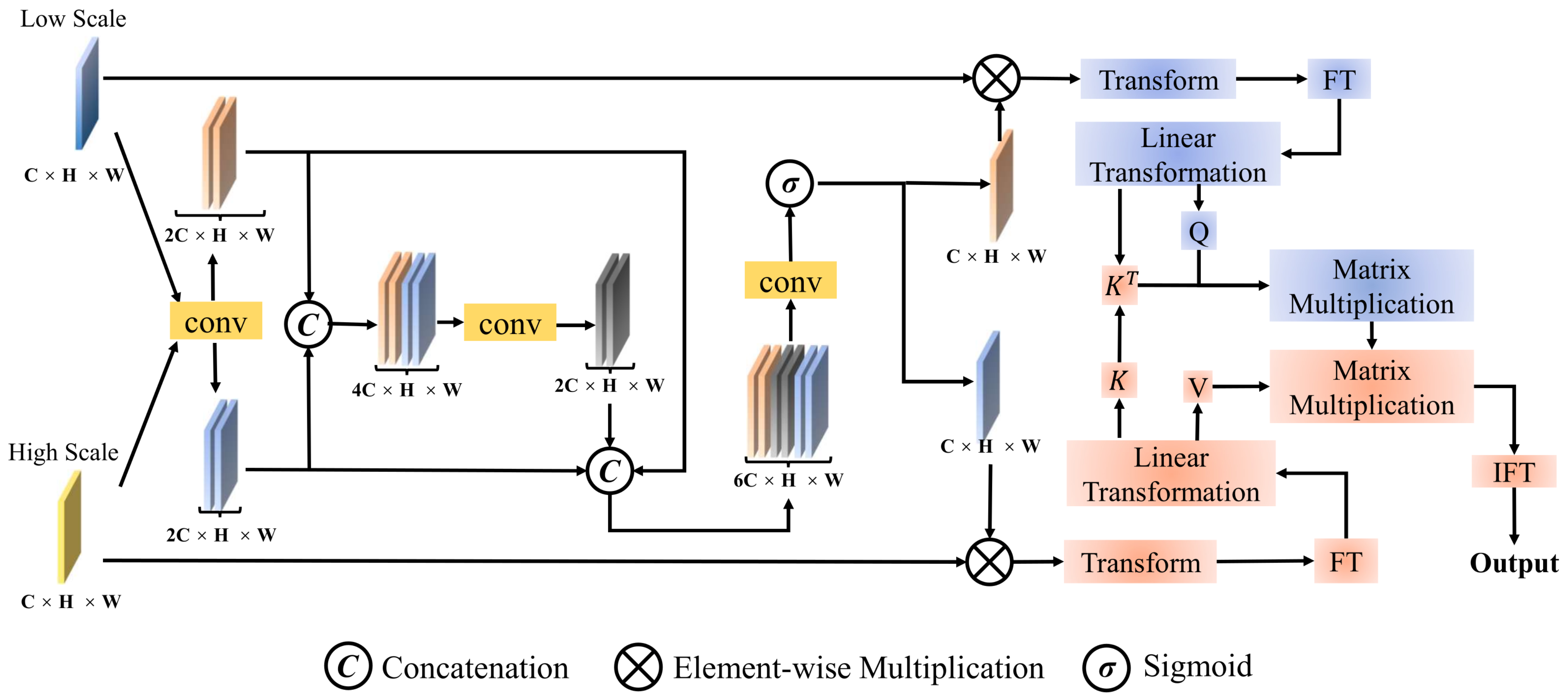
• A Transformer-based GHAT is introduced into the generative framework to integrate high-dimensional CD features into the diffusion noise domain. Simultaneously, low-dimensional CD features are utilized to calibrate prior CD results at each iterative step, progressively refining the generated outcomes. These integration operations effectively enhance noise prediction, resulting in high-precision CD results.

The remainder of this paper is structured as follows: Section 2 surveys the existing literature on DL-based CD methods and recently proposed DDPM architectures. Section 3 delineates the architectural and operational details of IMDCD. After that, extensive experimental results and evaluations are subsequently conducted in Section 4, culminating in concluding remarks in Section 5.

2. Related Works

2.1. Traditional DL-Based Models in CD

CNNs have emerged as a cornerstone in advancing CD methods [35]. They are particularly adept at unraveling complex spatial patterns [36], which is essential for accurate CD. Innovations like the Symmetric Convolutional Coupling Network (SCNN) have enhanced our understanding of image relationships. The Recurrent Convolutional Neural Network (ReCNN) [37] is particularly adept at bridging temporal gaps in datasets. Deep Neural Networks (DNNs), including Siamese networks and Fully Convolutional Networks (FCNNs) with Unet architectures [13], have enhanced CD accuracy through multi-scale feature extraction. Although DNN-based algorithms have widened the scope of CD, they struggle with spatial–temporal information capture, especially when dealing with shrinking image patch sizes. Other groundbreaking models include the Local–Global Pyramid Network (LGPNet) [38] and Deeply Supervised Image Fusion Network (DSIFN) [39], both designed for comprehensive feature extraction. The introduction of attention mechanisms in the Double Attentive Siamese Network (DASNet) [40] marks another step forward in refining feature extraction. DSN introduces a Siamese network structure to tackle the problem of change detection in remote sensing images as a binary semantic segmentation task [41]. DTM utilizes multi-spectral and SAR data to facilitate automated and continuous urban-change monitoring across different periods and locations without manual sample selection [42].

However, the aforementioned CNN-based models often struggle to capture global dependencies, especially in the context of complex and extensive changes [43].

To cope with the aforementioned challenges, the emergence of Transformers has been recognized as a promising approach [22]. Their ability to manage long-range dependencies through self-attention modules allows them to capture global contextual relationships effectively. For instance, SwinsUnet leverages Swin Transformer blocks [44] to improve global representation, addressing the limitations of CNNs related to their receptive field. The development of Transformer-based models for CD is a clear indication of their superiority in processing global information [45]. MFATNet integrates multi-scale features with a focus on semantic depth, facilitated by the Transformer architecture to enhance change detection in remote sensing images [46]. EGCTNet proposes edge guidance with hybrid CNN-Transformer architectures to refine and enhance feature detection in remote sensing change-detection tasks [47].

Despite their advantages, Transformers occasionally struggle with local variations and the precise delineation of change boundaries, an area where further refinement is urgently required.

2.2. DDPM-Based Models in CD

DDPMs [33] stand out in synthesizing high-quality images by iteratively diffusing noise through a series of steps. Through a combination of learned denoising functions and a generator network, the DDPM effectively captures complex image distributions, making it valuable for tasks like image generation, denoising, and restoration across various domains.

DDPMs offer a significant leap forward in CD, particularly when compared to traditional CNNs and Transformers [48]. Their diffusion mechanisms enable the superior handling of complex data distributions, resulting in more precise fine-grained detail and edge representation in CD maps [49]. The foundational principle of DDPMs involves transforming a standard normal distribution into an empirical data distribution. DDPM-CD [50], a variant model for semantic segmentation and CD tasks, utilizes the DDPM as a feature extractor. This approach effectively minimizes information loss by harnessing the strengths of the diffusion model. Nevertheless, the full potential exploitation of the DDPM, especially in progressive learning and iterative refinement, is an area that remains underexplored. The GCD-DDPM [32], depicted in Figure 1b, effectively leverages the multi-step inference process of the DDPM to generate a refined CD result. However, the CNN-based conditional encoder grapples with capturing long-frequency information within high-resolution RS images. To address this drawback, we design MCD as the conditional encoder, effectively capturing long-frequency information while maintaining the linear computation complexity.

2.3. Mamba-Based Models in CD

State Space Models (SSMs) have garnered significant attention among researchers, extending classical SSM research by incorporating long-distance dependencies and maintaining linear complexity concerning input size. Modern SSMs have found applications across various domains, including language understanding [51], general vision [52], and more.

Recently, with the first application of the Mamba architecture to CD tasks in ChangeMamba [31], numerous researchers have introduced the “Mamba” framework into the field of RS, yielding remarkably promising results. MLGTM proposed advanced geometric deep learning concepts and Transformer-Mamba techniques to address the unique challenges of point cloud classification [29]. RS-Mamba [53] is proposed for dense prediction tasks in large very-high-resolution RS images, achieving significant advancements in performance. To provide additional global information to the convolution-based main branch, RS3Mamba [54] is introduced, a novel dual-branch network that utilizes VSS blocks. In order to address the limitations of CNNs in remote modeling capabilities and the computational complexity constraints of Transformers, and drawing inspiration from the success of Vmunet [55], we chose the Mamba architecture as our encoder framework.

Overall, IMDCD addresses the limitations of existing methods and introduces significant advancements in CD technology. Specifically, traditional Transformer attention mechanisms, while effective at capturing global information, suffer from a high computational complexity and significant memory requirements. IMDCD integrates the Mamba architecture to maintain efficient long-distance dependency relationships, enhancing model efficiency. Moreover, compared with the ChangeMamba method limited by its single-pass propagation approach, the proposed model employs the DDPM framework. This allows for the iterative refinement of the change-detection map, enhancing the model’s ability to iteratively learn change-aware features and further improving its generalizability. Additionally, the proposed method overcomes the limitations of the GCD-DDPM’s reliance on CNN-based conditional encoders by employing a Swin-Mamba-Encoder (SME). IMDCD combined with Variable State Space CD (VSS-CD) and CD-yolo integration allows for effective long-dependency change computation and multi-scale feature integration, providing a comprehensive solution for precise change detection.

3. Methodology

3.1. Diffusion Model

DDPMs have become notable for producing high-quality images, outperforming traditional models such as GANs [56,57] and Variational Autoencoders (VAEs) [58,59]. These diffusion models are particularly adept at extracting semantic details from images, making them suitable for tasks like image segmentation and CD.

3.1.1. Training Stage

The training phase in the DDPM centers around optimizing the noise predictor parameters $\theta$. This is accomplished by minimizing the Mean Squared Error (MSE) loss function. The primary goal of this optimization is to train the model to effectively learn the reverse diffusion process, a pivotal aspect for successfully denoising the data.

In the forward process, noise is incrementally added to the data point $x_0$ at each time step t, generating a series of data points $x_1$, $x_2$, …, $x_T$ conditioned on a given initial data distribution $x_0\sim q\left(x_0\right)$. This process can be described by the Gaussian transition:

$$q\left(x_t\right|x_{t-1})=\mathcal{N}(x_t;\sqrt{1-{\beta }_t}{x}_{t-1},{\beta }_t{\mathbf{I}}_{n\times n}).$$

(1)

Here, $\mathcal{N}\left(·;·,·\right)$ represents a Gaussian distribution. The covariance matrix ${\beta }_t{\mathbf{I}}_{n\times n}$ incorporates the identity matrix ${\mathbf{I}}_{n\times n}$ of size $n\times n$, ensuring that noise is added independently to each dimension of $x_{t-1}$ with a variance of ${\beta }_t$.

The relationship between the original data point $x_0$ and the noised data at each step t is expressed as

$$x_t=\sqrt{{\overline{\alpha }}_t}{x}_0+\sqrt{1-{\overline{\alpha }}_t}ϵ,$$

(2)

with $ϵ$ being the standard Gaussian noise, i.e., $ϵ\sim \mathcal{N}(0,{\mathbf{I}}_{n\times n})$, and ${\overline{\alpha }}_t$ defined as ${\overline{\alpha }}_t={\prod }_{s=1}^t(1-{\beta }_s)$.

The reverse process, crucial for reconstructing the original data from its noised version, is defined as

$$p_{\theta }\left(x_{t-1}\right|x_t)=\mathcal{N}(x_{t-1};{\mu }_{\theta }(x_t,t),{\sigma }_{\theta }^2(x_t,t){\mathbf{I}}_{n\times n}),$$

(3)

where ${\mu }_{\theta }(x_t,t)$ and ${\sigma }_{\theta }^2(x_t,t)$ are functions parameterized by the neural network $\theta$, determining the mean and variance for the reverse transition.

The loss function used during training is often a simplification of the variational lower bound, which in many cases is the Mean Squared Error (MSE) between the predicted and the actual value of $x_{t-1}$ at each step of the reverse process:

$${\mathcal{L}}_{\mathrm{MSE}}\left(\theta \right)={\mathbb{E}}_{t,x_0,ϵ}\left[\parallel x_{t-1}-{\mu }_{\theta }(x_t,t){\parallel }^2\right].$$

(4)

This MSE loss is often supplemented with additional terms to ensure the model accurately learns the variance of the reverse transition.

3.1.2. Inference Stage

The inference stage of a diffusion model begins with a sample $x_T$ drawn from a standard Gaussian distribution, i.e., $x_T\sim \mathcal{N}(0,{\mathbf{I}}_{n\times n})$. The objective is to iteratively apply the learned reverse transitions to progressively denoise this sample, approximating the original data distribution. Mathematically, this is achieved through a series of steps, represented by

$$x_{t-1}={\mu }_{\theta }(x_t,t)+{\sigma }_{\theta }(x_t,t)·z_{t-1},t=T,T-1,\cdots ,1,$$

(5)

where ${\mu }_{\theta }(x_t,t)$ and ${\sigma }_{\theta }(x_t,t)$ are the outputs of the neural network for the mean and standard deviation of the reverse transition. The term $z_{t-1}$ is a noise sample drawn from $\mathcal{N}(0,{\mathbf{I}}_{n\times n})$, which is gradually reduced as t decreases.

This iterative process continues until $x_0$ is reached, which is the model’s best estimate of the original uncorrupted data. This step-by-step denoising effectively reverses the forward diffusion process, enabling the generation of high-quality samples from the learned data distribution.

3.2. Network Details

As illustrated in Figure 2, a hybrid Transformer–convolutional structure is designed as the noise predictor, which is conditioned on CD features extracted from MCD, as expressed by

$${ϵ}_{\theta }(x_t,I^a,I^b,t)=D\left(\mathrm{GHAT}(E(m^{LC}+P\left(x_t\right),t),m^{HC}),t\right),$$

(6)

where $m^{HC}$ and $m^{LC}$ represent the high- and low-dimensional CD conditions from MCD, respectively. Both conditions are extracted from the RS images $I^a$ and $I^b$. The function $P(·)$ is a convolutional layer designed to encode the noise $x_t$, thereby generating a CD noise feature. The CD noise feature is represented as $P\left(x_t\right)$ within the space ${\mathbb{R}}^{64\times H\times W}$. Initially, the feature $P\left(x_t\right)$ undergoes a conditioning process by $m^{LC}$, after which it is encoded by the DDPM-Encoder denoted as E. This encoded feature is subsequently integrated with the high-dimensional CD condition $m^{HC}$ through the GHAT mechanism. The attention mechanism refines the integration process and outputs an Attention Change feature map, referred to as $m_{AC}$, which is then relayed to the DDPM-Decoder, symbolized as D, to obtain the CD-related noise.

Specifically, given RGB pre- and post-change images $I_a\in {\mathbb{R}}^{H\times W\times 3}$ and $I_b\in {\mathbb{R}}^{H\times W\times 3}$, a Mamba-Encoder within MCD extracts multi-level features from each image. The downsampled conditional feature maps $m_i^a$ and $m_i^b$ produced by the i-th SME layer are of size $C_i\times {\displaystyle \frac{H}{2^{i-1}}}\times {\displaystyle \frac{W}{2^{i-1}}}$, where i is the layer index with $i=1,2,\dots ,5$, and $C_i=64\times i$. These semantic features $(i=2,\dots ,5)$ of $I_a$ and $I_b$ are conveyed into VSS-CD to compute informative change features $m_i^{CD}\in {\mathbb{R}}^{C_i\times {\displaystyle \frac{H}{2^{i-1}}}\times {\displaystyle \frac{W}{2^{i-1}}}}$, $i=2,\dots ,5$, where $m_5^{CD}$ denotes the highest-dimension change feature map $m^{HC}$, which will be integrated into the GHAT as the high-dimensional CD condition. Extracted change features are fused and upscaled by a CD-yolo module in MCD to obtain the lowest-dimension change feature map with precise edge details, denoted as $m^{LC}\in {\mathbb{R}}^{64\times H\times W}$. Element-wise addition is employed to fuse the $m^{LC}$ and $P\left(x_t\right)$. The details of the SME is shown in

Table 1. Structure of Swin-Mamba-Encoder (each encoder).

Stage	Outputs
Convolution	${\displaystyle \frac{H}{2}}\times {\displaystyle \frac{W}{2}}\times C$
Linear Embedding + VSS Blocks $\times 2$	${\displaystyle \frac{H}{4}}\times {\displaystyle \frac{W}{4}}\times C$
Patch Merging + VSS Blocks $\times 2$	${\displaystyle \frac{H}{8}}\times {\displaystyle \frac{W}{8}}\times 2C$
Patch Merging + VSS Blocks $\times 2$	${\displaystyle \frac{H}{16}}\times {\displaystyle \frac{W}{16}}\times 4C$
Patch Merging + VSS Blocks $\times 2$	${\displaystyle \frac{H}{32}}\times {\displaystyle \frac{W}{32}}\times 8C$

.

Upon incorporating $m^{LC}$ into the DDPM, the conditioned CD noise feature is encoded by the DDPM-Encoder in the DDPM, represented as $E(m^{LC}+P\left(x_t\right),t)$. This encoded feature is further fused with $m^{HC}$ by the proposed GHAT module and seamlessly conveyed into the DDPM-Encoder within the DDPM to finally obtain the CD-related noise ${ϵ}_{\theta }(x_t,I^a,I^b,t)$.

The estimated noise is then leveraged to facilitate the sampling process each step iteratively, based on the equations, obtaining

$$x_{t-1}={\displaystyle \frac{1}{\sqrt{{\alpha }_t}}}\left(x_t-{\displaystyle \frac{1-{\alpha }_t}{\sqrt{1-{\overline{\alpha }}_t}}}{ϵ}_{\theta }(x_t,I^a,I^b,t)\right)+{\sigma }_{\theta }(x_t,t)z,$$

(7)

where $z\sim \mathcal{N}(0,{\mathbf{I}}_{\mathbf{n}\times \mathbf{n}})$. Through 1000 iterations of sampling [50], the single-channel CD map is ultimately generated and sampled from a 2D Gaussian noise distribution.

3.2.1. Mamba-CD Feature Extractor Module

To extract global semantic information from images while maintaining linear complexity, we introduce the Mamba-based module, termed MCD, effectively improving the change-detection accuracy. This module processes pre- and post-change images, represented as $I_a\in {\mathbb{R}}^{H\times W\times 3}$ and $I_b\in {\mathbb{R}}^{H\times W\times 3}$, respectively. Specifically, MCD employs the SME, with five stages for extracting multi-scale features, to obtain multi-scale features from image sets. The extracted feature maps at various levels are denoted as $m_i^a$ for $I_a$ and $m_i^b$ for $I_b$, where the i-th level is for $i=1,2,\dots ,5$. Specifically, the first stage involves a convolution layer that performs 2× downsampling, reducing the spatial dimensions of the input images $I_a$ and $I_b$, formulated as

$$m_1^a={\mathrm{Conv}}_{7\times 7}^{s=2,p=3}\left(I_a\right)\mathrm{and}{m}_1^b={\mathrm{Conv}}_{7\times 7}^{s=2,p=3}\left(I_b\right),$$

where ${\mathrm{Conv}}_{7\times 7}^{s=2,p=3}$ denotes a convolution operation with a 7 × 7 kernel, stride s of 2, and padding p of 3. This operation effectively halves the resolution of the input images.

Moreover, from stages two to five, the downsampling is primarily conducted through a patch-merging layer, which consistently reduces the spatial resolution by a factor of 2× at each stage. The specific transformation at each stage i (for $i=2,3,4,5$) for both pre- and post-change images can be mathematically detailed as follows:

$$m_i^a=\mathrm{PatchMerge}\left(m_{i-1}^a\right)\mathrm{and}{m}_i^b=\mathrm{PatchMerge}\left(m_{i-1}^b\right),$$

where PatchMerge represents the patch-merging operation that combines adjacent patches (each patch representing a specific feature vector) into a single, larger patch. This operation not only reduces the dimensionality but also helps in aggregating local features into more global representations, crucial for detecting changes across images. The output at each stage further undergoes processing through VSS blocks for enhanced feature extraction.

Sequentially, we further innovate the SSM to make it more suitable for the CD task, which focuses on emphasizing the differences between sequential images. We propose the SS-CD (State Space Change Detection) module, which focuses on the difference values between pre-change and post-change images. Specifically, the SS-CD is a linear time-invariant system function to map the difference between the pre-change and post-change images through a hidden state $h\left(t\right)\in {\mathcal{R}}^N$ given $A\in {\mathcal{C}}^{N\times N}$ as the evolution parameter, $B,C\in {\mathcal{C}}^N$ as the projection parameters for a state size N, and skip connection $D\in {\mathcal{C}}^1$. The model can be formulated as a linear ordinary differential equation as

$$\begin{array}{c}\hfill h^{\prime }\left(t\right)=Ah\left(t\right)+B(m_i^b-m_i^a).\end{array}$$

(8)

$$\begin{array}{c}\hfill y\left(t\right)=Ch\left(t\right)+D(m_i^b-m_i^a).\end{array}$$

(9)

The discrete version of this linear model can be transformed by the zero-order hold given a timescale parameter $\Delta \in {\mathcal{R}}^D$, represented by

$$\begin{array}{cc}\hfill h_t& =\overline{A}{h}_{k-2}+\overline{B}x,\hfill \\ \hfill y_t& =C{h}_k+\overline{D}{x}_k,\hfill \\ \hfill \overline{A}& =e^{▵A},\hfill \\ \hfill \overline{B}& =(e^{▵A}-\mathbf{I})A^{-1}B,\hfill \\ \hfill \overline{C}& =C.\hfill \end{array}$$

(10)

The approximation of B is refined using the first-order Taylor series $\overline{B}=(e^{\Delta A}-\mathbf{I})A^{-1}B\approx (\Delta A){(\Delta A)}^{-1}\Delta B=\Delta B$.

As shown in Figure 3, the VSS-CD block processes the input feature through a linear embedding layer before bifurcating into dual pathways. One pathway proceeds through depth-wise convolution [60] and SiLU activation [61], leading to the SS-CD module as a bridge, linking the pre-change and post-change CD images. Subsequently, post-layer normalization is applied, followed by integration with the alternate pathway post-SiLU activation for the other portion of the difference information. The SS-CD module functions as a sophisticated mechanism to distill the essence of change within a data stream, particularly focusing on capturing subtle and nuanced alterations over extended periods. Consequently, it ensures that the CD process is both accurate and comprehensive in its assessment of the evolving data landscape. After processing by the SS-CD module, the differences are then fed into the DDPM, enhancing the overall analysis.

The number of channels in each subsequent stage of the encoder is increased as the spatial dimensions are reduced.

Inspired by [55], we propose the SME to tackle the problem of precisely detecting and outlining changes in intricate, high-dimensional image data. The input image, denoted by ${\mathbb{R}}^{H\times W\times 3}$, is initially processed through a convolution layer, effectively halving both the height and width (resulting in ${\displaystyle \frac{H}{2}}\times {\displaystyle \frac{W}{2}}\times C$), where C represents the channel dimension at this initial stage. This convolution is followed by a linear embedding process paired with Vision Swin Sequence (VSS) blocks, which further condense the spatial dimensions to ${\displaystyle \frac{H}{4}}\times {\displaystyle \frac{W}{4}}\times C$. Subsequent stages in the encoder involve a series of patch-merging operations coupled with additional VSS blocks that continuously compress the spatial dimensions while increasing the number of channels. The strategy of channel increasing effectively compensates for the loss of spatial information and improves the network’s capacity to represent features more comprehensively. By capturing more complex patterns and details in the data, the network is better equipped to represent high-level semantic information, which is crucial for accurate and detailed image analysis. The third stage results in an output of ${\displaystyle \frac{H}{8}}\times {\displaystyle \frac{W}{8}}\times 2C$, the fourth stage produces ${\displaystyle \frac{H}{16}}\times {\displaystyle \frac{W}{16}}\times 4C$, and the fifth stage culminates in a resolution of ${\displaystyle \frac{H}{32}}\times {\displaystyle \frac{W}{32}}\times 8C$. Each of these stages incorporates two instances of VSS blocks to enrich the feature-extraction process, ensuring a deep and complex representation suitable for high-precision change detection.

Moreover, we employ the CD-yolo module as the decoder of the model. Inspired by the head and neck parts of YOLOv8, the CD-yolo module incorporates advanced techniques to enhance feature integration for CD. The design includes a series of upsampling, concatenation, C2f, and convolution operations, which work together to effectively integrate CD features from SS-CD at different scales. By leveraging these operations, the CD-yolo module improves the model’s ability to capture and combine multi-scale features, thereby enhancing the Overall Accuracy and performance of the CD process.

The CD-yolo module, serving as the decoder part of the model, integrates features from different layers through upsampling and concatenation, ensuring a comprehensive analysis at various scales. Its core component, the C2f module, utilizes $3\times 3$ convolutional kernels within Bottleneck layers to extract and refine feature information. As these features progress through interconnected Bottleneck layers, they evolve from basic to complex feature maps, balancing intricate details and contextual information. Residual connections within the C2f module enable the leveraging of both fine-grained details and the broader context, enhancing the accuracy and robustness of feature integration.

By integrating these components, the CD-yolo module optimally fulfills its role as a decoder, ensuring that the CD process leverages both detailed and contextual features to yield more precise and reliable outcomes.

3.2.2. NEUNet Architecture and Functionality

The NEUNet consists of the DDPM-Encoder, the GHAT module, and the DDPM-Decoder. This setup effectively combines low- and high-dimensional CD conditions to produce refined CD-related noise. The $DPM$-$Encoder$ is tasked with enriching the conditioned CD noise features, denoted as $m_n^k$, through four Residual blocks at levels $k=2,3,4,5$. Each block uses downsample layers for reducing dimensions, employing a $2\times 2$ convolutional layer with stride 2, preceded by layer normalization. Starting with a dimension of $64\times H\times W$ after the initial layer, the encoder applies successive $2\times$ downsampling, resulting in feature dimensions of $128\times {\displaystyle \frac{H}{2}}\times {\displaystyle \frac{W}{2}}$, $192\times {\displaystyle \frac{H}{4}}\times {\displaystyle \frac{W}{4}}$, and $256\times {\displaystyle \frac{H}{8}}\times {\displaystyle \frac{W}{8}}$ at each subsequent stage. The final stage outputs $m_n^5$, a feature map with a dimension of $320\times {\displaystyle \frac{H}{16}}\times {\displaystyle \frac{W}{16}}$ after processing through the ResNet-inspired encoder.

Furthermore, to overcome the challenge of merging high-level CD conditions with noise features effectively, we introduce the GHAT. As illustrated in Figure 4, this component is carefully designed to ensure a seamless and coherent union of the high-dimensional CD condition $m^{HC}$ with the encoded conditioned CD noise feature $m_n^5$. Specifically, we double the number of channels on both inputs through a 1 × 1 convolution operation, which can be defined as

$$M^l={\mathrm{conv}}^{1\times 1}\left(m_n^5\right),M^h={\mathrm{conv}}^{1\times 1}\left(m^{HC}\right),$$

(11)

while $M^l$ and $M^h$ represent the refined feature map after extending the channel. Subsequently, we concatenate the two feature maps, effectively combining their respective information, which can be represented as

$$M^{fuse}={\mathrm{conv}}^{1\times 1}\left([M^l,M^h]\right),$$

(12)

where $[·]$ represents the concatenation and $M^{fuse}$ represents the first intermediate feature map. Following this, we average the two refined feature maps simultaneously to obtain the aligned global features and then splice the aforementioned three feature maps together as follows:

$${\mathcal{M}}^{fuse}=[Avg\left(M^l\right),Avg\left(M^h\right),F^{Muse}],$$

(13)

where $Avg(·)$ represents the operation of calculating the mean value of a feature map and expanding it over the entire pixel space. This operation aims to obtain global features that capture the overall properties of the input features. ${\mathcal{M}}^{fuse}$ represents the second intermediate feature map. After concatenating the three feature maps, we apply a $1\times 1$ convolution operation followed by a sigmoid function. This process yields two different global attention feature maps with enhanced global semantic information, one at a low scale and the other at a high scale:

$$M_{att}^l,M_{att}^h=\sigma \left({\mathrm{Conv}}^{1\times }\left({\mathcal{M}}^{fuse}\right)\right),$$

(14)

where $M_{att}^l$ and $M_{att}^h$ represent the global attention feature maps of low and high scales, respectively. Then, we multiply the two attentional feature maps element-wise with the original input feature map as

$${\mathcal{M}}^{low}=m_n^5\otimes M_{att}^l,{\mathcal{M}}^{high}=m^{HC}\otimes M_{att}^h.$$

(15)

Subsequently, ${\mathcal{M}}^{high}$ and ${\mathcal{M}}^{low}$ are transformed into token representations $H\in {\mathbb{R}}^{256\times 320}$ and $L\in {\mathbb{R}}^{256\times 320}$, respectively. These tokens undergo Fourier Transform (FT), which converts the spatial domain features into their frequency domain representations. This strategy enables the model to efficiently capture both global and local features from the image data. The tokens are then processed with query, key, and value weight matrices $W_q$, $W_k$, and $W_v$, resulting in Q, K, and V as shown below:

$$Q=FT\left(H\right)W_q,K=FT\left(L\right)W_k,V=FT\left(L\right)W_v.$$

(16)

Subsequently, a cross-attention mechanism computes the interaction between H and L, with the attention weights captured by

$$AC=IFT\left(SV\right)=IFT\left(\mathsf{\Phi }\left({\displaystyle \frac{Q{K}^T}{\sqrt{d_k}}}\right)V\right),$$

(17)

where $IFT(·)$ denotes the Inverse Fourier Transform (IFT), ensuring that the learned global and local patterns can be reapplied to the original image structure. $\mathsf{\Phi }(·)$ is the SoftMax function. The transposed matrix of K is given by $K^T$, with $d_k=320$ representing the dimensionality of the keys. The symbol S indicates the weighting parameters across all channels, and the resulting Attention Change Token $AC\in R^{256\times 320}$ incorporates channel-specific weightings.

Finally, the Attention Change Token $AC$ is transformed by the reconstruction module into an Attention Change feature map $m^{AC}$, which has the dimensions $320\times {\displaystyle \frac{H}{16}}\times {\displaystyle \frac{W}{16}}$. In essence, the fusion process within the GHAT yields the feature map $mAC$. Starting with $m_n^k\in {\mathbb{R}}^{320\times {\displaystyle \frac{H}{16}}\times {\displaystyle \frac{W}{16}}}$—the output from the encoder’s final stage—the decoder utilizes upsampling layers that feature transposed convolution operations with a $2\times 2$ kernel and stride of 2. This convolution process within the DDPM-Encoder expands the dimensions to $1\times H\times W$. The NEUNet’s robust architecture facilitates a streamlined progression from encoding through fusion to decoding. This seamless operational flow is what renders NEUNet an essential tool for precise noise estimation in sophisticated CD tasks. By intricately modeling and adjusting the noise, NEUNet significantly enhances the accuracy and dependability of the resulting CD map.

4. Performance Evaluation

4.1. Experimental Dataset

We conducted extensive experiments on four datasets for CD evaluation:

WHU [62], LEVIR [63], the CD dataset (CDD) [64], and OSCD [65].

• CDD: The CDD is a high-resolution, four-season dataset designed for image-change-detection tasks. It provides an exceptionally high spatial resolution and high-resolution RGB imagery obtained from Google Earth, ranging from 3 to 100 cm/pixel, delivering highly detailed imagery essential for accurate and in-depth analysis. The CDD includes 10,000 training images, 3000 testing images, and 3000 validation images, all with dimensions of $256\times 256$ pixels. The inclusion of images from different seasons ensures diversity and robustness in detecting changes under various seasonal conditions. The CDD’s comprehensive and high-resolution imagery makes it an ideal resource for developing and evaluating algorithms in the field of computer vision, particularly for change-detection applications.
• WHU: WHU comprises high-resolution aerial imagery with a spatial resolution of $7.5$ cm/pixel, making it suitable for detailed analysis in various computer vision tasks. The dataset is divided into 6096 training patches, 762 testing patches, and 762 validation patches, each with dimensions of $256\times 256$ pixels. This structured division ensures a comprehensive and systematic approach to model training, testing, and validation. The high-resolution imagery provided by the WHU dataset facilitates the development and evaluation of advanced algorithms for applications such as image classification, segmentation, and change detection.
• LEVIR: LEVIR is a large-scale building CD dataset characterized by a high spatial resolution of $0.5$ m. It is meticulously segmented into 7120 training patches, 1024 validation patches, and 2048 testing patches, each with dimensions of $256\times 256$ pixels. The high resolution and comprehensive segmentation of the LEVIR dataset make it an invaluable resource in the field of RS.
• OSCD: OSCD is specifically designed to capture urban changes, including the emergence of new buildings and roads. Despite being a low-spatial-resolution dataset between 10 and 60 m, it is effectively structured into 14 training pairs and 10 test pairs with 13 spectral bands. This configuration makes the OSCD dataset particularly suitable for the development and evaluation of CD algorithms in the context of RS. Its focus on urban environments makes the OSCD dataset a valuable dataset for advancing the accuracy and efficiency of CD techniques in monitoring urban growth and infrastructure development.

4.2. Implementation Details

Our experiments were conducted using the PyTorch framework on a single NVIDIA GeForce RTX 3090 Ti GPU, ensuring robust computational power and efficient processing. We performed a total of 1000 diffusion steps during the inference phase to achieve detailed and accurate results. For consistency and comparability, all images were uniformly resized to a dimension of $256\times 256$ pixels.

The optimization of our model was carried out using the Stochastic Gradient Descent (SGD) algorithm with momentum, a widely recognized method for its efficiency in converging to optimal solutions. We trained the model with a batch size of 32, which provided a good balance between the computational efficiency and the stability of the gradient estimates.

We set the momentum parameter to 0.99 to help the optimization process maintain a high level of directionality while the weight decay parameter was set to 0.0005 to prevent overfitting by penalizing large weights. The initial learning rate was configured to 0.0001, ensuring gradual and controlled learning. This rate was linearly decayed to zero over the course of 200 epochs, allowing the model to fine-tune its parameters progressively and stabilize toward the end of training.

These settings were chosen to ensure that our training process was both effective and efficient, leveraging the strengths of the hardware and the optimization algorithm to achieve a high performance in CD tasks.

4.3. Evaluation Metrics

In CD analysis, the efficacy of models is commonly evaluated using metrics like the F1 Score, Intersection over Union (IoU), and Overall Accuracy (OA). These metrics are crucial as they assess different and complementary aspects of CD model performance.

The F1 Score is the harmonic mean of precision and recall, considering both the accuracy and the coverage of the classification model for the positive class. Precision is the proportion of pixels predicted as change areas that are actually change areas, while recall is the proportion of actual change-area pixels that are correctly predicted as change areas. The formula for the F1 Score is

$$\mathrm{F}1=2\times {\displaystyle \frac{\mathrm{Precision}\times \mathrm{Recall}}{\mathrm{Precision}+\mathrm{Recall}}}.$$

(18)

A high F1 Score indicates a good balance between identifying change areas accurately and minimizing false positives.

The Intersection over Union (IoU) measures the overlap between the predicted change areas and the actual change areas, which is particularly useful for image segmentation and CD tasks. It is defined as the ratio of the intersection of the predicted and actual change areas to their union:

$$\mathrm{IoU}={\displaystyle \frac{\mathrm{TP}}{\mathrm{TP}+\mathrm{FP}+\mathrm{FN}}}.$$

(19)

True positives (TPs) are the number of pixels correctly identified as change areas, False Positives (FPs) are the number of pixels incorrectly identified as change areas, and false negatives (FNs) are the number of pixels that are actually change areas but not identified as such. A high IoU value indicates a high degree of overlap between the predicted and actual change areas, reflecting the precision and comprehensiveness of the prediction.

The Overall Accuracy (OA) is the proportion of correctly classified pixels out of the total number of pixels, providing a simple and intuitive measure of the model’s overall classification performance. It is calculated as

$$\mathrm{OA}={\displaystyle \frac{\mathrm{TP}+\mathrm{TN}}{\mathrm{TP}+\mathrm{TN}+\mathrm{FN}+\mathrm{FP}}},$$

(20)

where TN denotes true negatives. The Overall Accuracy evaluates the correctness of all classes (change and no-change), but it may be biased toward the majority class (the no-change areas) in cases of class imbalance.

These metrics collectively provide a robust framework for assessing the performance of CD models, considering both the detection accuracy and the precision of the identified changes.

4.4. Comparison

The proposed IMDCD method was compared against five state-of-the-art models: FC-SC [12] and SNUNet [66] (convolution-based), BIT [22] and ChangeFormer [67] (Transformer-based), and DDPM-CD [50] and GCD-DDPM [32]. FC-SC employs a Siamese Fully Convolutional Network for feature extraction. SNUNet combines the Siamese network with NestedUNet [68] for high-resolution feature extraction. BIT integrates Transformer architecture for CD, focusing on relevant changes. ChangeFormer employs a hierarchical Transformer encoder in a Siamese setup with a Multi-Layer Perceptron decoder, while IMDCD leverages the SME for feature extraction and the GHAT for integrating the extracted features into the end-to-end NEUNet.

4.5. Experiments on CDDs

The CDD is designed to capture seasonal variations in RS images, providing a robust platform for developing and evaluating CD algorithms. The dataset encompasses a range of land-cover and land-use types, such as urban areas and agricultural fields, captured across different seasons. Figure 5a–c display pre-change and post-change images alongside ground truth data, illustrating a range of land-cover and land-use types. Seasonal changes in vegetation and other land-cover types can lead to pseudo-changes in the CD maps, complicating the differentiation between actual changes and those induced by seasonal variability. This diversity supports a comprehensive assessment of CD algorithms across various spectral characteristics and scenarios.

Figure 5d–i show the predictive capabilities of the evaluated methods. For example, ChangeFormer tends to overestimate change areas, leading to noise, as seen in Figure 5g. The GCD-DDPM employed the diffusion model within the CD task, providing precise detection boundaries through multi-step inference but resulting in some omissions, as shown in Figure 5h. The proposed IMDCD exhibits an extraordinary performance in environments with clear, defined changes such as new construction within urban settings, as depicted in row 3 of Figure 5. The algorithm effectively captures the geometrical changes and differentiates between pre- and post-change images with high precision. Conversely, the performance is less optimal in scenarios where changes are small-scale or within naturally cluttered landscapes, such as the subtle vehicle alterations shown in row 2.

Overall, as demonstrated in Figure 5i, IMDCD addresses most of the complex conditions while preserving more detailed prediction results.

Table 2. The quantitative experimental results (%) on the CDD. The values in bold are the best.

Method	Recall	Precision	OA	F1	IoU
FC-SC [12]	71.10	78.62	94.55	74.67	58.87
SNUNet [66]	80.29	84.52	95.73	82.35	69.91
BIT [22]	90.75	86.38	97.13	88.51	79.30
ChangeFormer [67]	93.64	94.54	98.45	94.09	88.94
GCD-DDPM [32]	95.10	94.76	98.87	94.93	90.56
IMDCD	96.73	97.49	99.34	97.11	94.12

compares the performance of the six models in terms of the OA, F1 Score, precision, and IoU. An examination of Table 2 reveals that the proposed IMDCD outperforms others in all metrics.

4.6. Experiments on WHU Datasets

We extended experiments to the WHU building CD dataset to further validate the effectiveness of the proposed IMDCD method. The WHU dataset, which focuses on urban changes such as construction, demolition, and land-cover transformations, presents unique challenges due to its intricate urban structures and diverse land-cover types. These complexities often lead to pseudo-changes and misclassifications in CD maps.

The visual results in Figure 6 and the quantitative metrics in

Table 3. The quantitative experimental results (%) on WHU. The values in bold are the best.

Method	Recall	Precision	OA	F1	IoU
FC-SC [12]	86.54	72.03	98.42	78.62	64.37
SNUNet [66]	81.33	85.66	98.68	83.44	71.39
BIT [22]	87.94	89.98	99.30	88.95	81.53
ChangeFormer [67]	86.43	89.69	98.95	88.03	78.46
GCD-DDPM [32]	92.29	92.79	99.39	92.54	86.52
IMDCD	93.27	93.85	99.51	93.56	88.39

reveal the limitations of other methods in urban CD. For example, methods like SNUNet and BIT, despite their higher recall values, show an overdetection of changes and lower precision, resulting in numerous misclassified areas, as seen in Figure 6e,g. While the GCD-DDPM method produces cleaner change detection with fewer false positives compared to SNUNet and BIT, it still struggles to capture the full spectrum of urban changes, leading to occasional omissions of subtle changes, as shown in Figure 6i. In contrast, the proposed IMDCD method excels in mitigating noise and pseudo-changes, effectively preserving the internal compactness and boundaries of urban objects. This robustness is reflected in its superior performance in key metrics, such as the F1 Score, OA, and IoU, as compared to other existing methods. The IMDCD method consistently demonstrated its ability to accurately detect urban changes, confirming its advantages both qualitatively and quantitatively.

4.7. Experiments on LEVIR Datasets

Next, we conducted similar experiments on the LEVIR-CDD, designed specifically for detecting building changes across various scales. As illustrated in Figure 7, the proposed IMDCD model demonstrates a superior performance by effectively preserving the internal structure of building objects while efficiently mitigating noise, contrasting with other existing models. Notably, the presence of seasonal and illumination variations in the bitemporal images often introduces significant spectral variability, resulting in pseudo-changes evident in the CD maps. This challenge is particularly pronounced in the case of small building targets, where pseudo-changes appear on building roofs while numerous small targets are overlooked. In contrast, the proposed IMDCD model adeptly detects the majority of small targets while simultaneously suppressing pseudo-changes, and it outperformed other methods across multiple metrics (

Table 4. The quantitative experimental results (%) on LEVIR. The values in bold are the best.

Method	Recall	Precision	OA	F1	IoU
FC-SC [12]	77.29	89.04	98.25	82.75	69.95
SNUNet [66]	84.33	88.55	98.70	86.39	76.11
BIT [22]	87.85	90.26	98.83	89.04	80.12
ChangeFormer [67]	87.73	89.39	98.81	88.56	79.34
GCD-DDPM [32]	91.24	90.68	99.14	90.96	83.56
IMDCD	91.12	91.56	99.21	91.34	84.66

).

4.8. Experiments on OSCD Datasets

The OSCD dataset [65], featuring low-resolution multi-spectral images of urban and natural landscapes, tested the effectiveness of IMDCD. It demonstrated a remarkable performance by distinguishing actual changes from pseudo-changes, particularly in highly structured urban environments, as seen in scenarios with extensive area changes depicted in row 2 of Figure 8. IMDCD achieves the best balance between precision and recall and is quantitatively supported by the leading IoU and F1 Score metrics (

Table 5. The quantitative experimental results (%) on OSCD. The values in bold are the best.

Method	Recall	Precision	OA	F1	IoU
FC-SC [12]	54.83	47.97	94.55	51.17	34.33
SNUNet [66]	60.49	48.62	94.63	53.91	36.13
BIT [22]	50.09	65.64	94.63	56.82	40.26
ChangeFormer [67]	49.37	62.90	95.20	55.32	38.10
GCD-DDPM [32]	73.94	50.60	95.84	60.08	43.29
IMDCD	58.39	67.21	96.37	62.49	45.52

), confirming the model’s high accuracy and establishing it as a new benchmark in CD, especially in low-resolution scenarios. At the same time, the visual results depicted in Figure 8 demonstrate that compared to other methods, the proposed IMDCD exhibits a superior detection performance.

However, the detection results are not ideal in more complex, natural settings where the changes are subtle or dispersed across a cluttered background, as illustrated in row 1 of Figure 8. In these cases, the algorithm tends to predict many extraneous noise points, complicating the accurate identification of real changes.

4.9. Multi-Scale Feature Visualization with Heatmaps

To demonstrate the performance improvements of IMDCD, Gradient-weighted Class Activation Mapping (Grad-CAM) [69] was used to visualize the feature map outputs from the decoder layer. As shown in Figure 9, we utilize heatmaps to visualize the multi-scale features detected by our model across various aerial images, including both urban and natural landscapes. These precious visualization results intuitively demonstrate the powerful capability of IMDCD to extract distinctive information from complex scenes. However, challenges arise in scenes rich with complex semantic elements, such as dense tree coverage, where the heatmaps display diminished activity. The findings highlight the need for enhanced model robustness against complex semantic disturbances, guiding future improvements in algorithmic adaptability to diverse environmental contexts.

4.10. Ablation Study

We provide a detailed analysis of the ablation studies conducted to evaluate the incremental benefit of integrating various features and modules within our proposed framework. The ablation studies are designed to validate the efficacy of Variable State Space CD (VSS-CD) and the use of high-dimensional and low-dimensional features. These experiments are critical in demonstrating the individual and combined contributions of each component toward enhancing the model’s performance in change-detection tasks. Our ablation study comprises four different configurations, each assessed on the WHU dataset to ascertain their impact on the Overall Accuracy (OA), F1 Score, and Intersection over Union (IoU). The experimental configurations and their corresponding performances are detailed in

Table 6. Ablation experiment results (%) on the WHU dataset. The values in bold are the best.

VSS-CD	High-Dimensional	Low-Dimensional	OA	F1	IoU
	✓	✓	99.37	92.61	86.47
✓	✓		99.41	92.73	87.04
✓		✓	99.38	92.45	86.67
✓	✓	✓	99.51	93.56	88.39

and are visually supported by the comparative results shown in the Figure 10.

We first evaluate the model using both high-dimensional and low-dimensional features without the inclusion of VSS-CD. This setup serves as our baseline, against which the benefits of additional features are compared. The results indicate a solid performance with an OA of 99.37%, an F1 Score of 92.61%, and an IoU of 86.47%. Moreover, we incorporate VSS-CD while focusing on high-dimensional feature processing, which markedly enhances the model’s ability to detect subtle changes. This is evidenced by the improved performance metrics with an OA of 99.41%, an F1 Score of 92.73%, and an IoU of 87.04%. Furthermore, by applying VSS-CD to low-dimensional features, the model demonstrates a refined capacity to maintain essential spatial details, slightly enhancing the IoU to 86.67% while slightly decreasing the F1 Score, highlighting the trade-offs involved in feature selection. The full integration of VSS-CD with both high- and low-dimensional features showcases the superior capability of our proposed model, achieving the best results with an OA of 99.51%, an F1 Score of 93.56%, and an IoU of 88.39%. This configuration clearly illustrates the effectiveness of the proposed three enhancements.

4.11. Efficiency

Table 7. Comparison of computation complexity.

Method	GFLOPs (G)	Para (M)
FC-SC [12]	4.73	1.35
SNUNet [66]	13.79	3.01
Bit [22]	8.75	3.04
ChangeFormer [67]	202.7	41.02
GCD-DDPM [32]	269.50	130.80
IMDCD	183.7	91.23

presents a comparison of the computational complexity among various CD models. FC-SC [12] is the most resource-efficient method, with only 1.35 million parameters and a low computational cost of 4.73 GFLOPs. In contrast, more advanced models like ChangeFormer [67], GCD-DDPM [32], and the proposed IMDCD, while achieving higher accuracy, involve significant complexity. ChangeFormer requires 202.7 GFLOPs and 41.02 million parameters due to its Transformer architecture. The GCD-DDPM, leveraging the generative diffusion model, demands the highest resources with 269.50 GFLOPs and 130.80 million parameters. The proposed IMDCD achieves a balance between the computational efficiency and performance with 183.7 GFLOPs and 91.23 million parameters. The SME within IMDCD efficiently captures long-range dependencies and intricate spatial details without excessively increasing computational demands. This efficiency allows IMDCD to maintain a high performance in CD tasks while managing computational resources more effectively.

5. Conclusions

This paper presents a Mamba-based approach for CD with high-resolution RS data, termed IMDCD. This method effectively addresses the dual challenges of capturing both long-range dependencies and local spatial information. By incorporating the GHAT, IMDCD is adept at managing both high- and low-dimensional CD conditions. Additionally, the proposed VSS-CD overcomes the limitations of basic subtraction methods, enabling a more detailed extraction of change information. The integration of the MCD framework with the SME and CD-yolo further enhances the capability of the proposed method to extract semantic features between pre- and post-change images. Numerical experiments across diverse CD datasets such as the CDD, WHU, LEVIR, and OSCD demonstrate the superiority of IMDCD in generating accurate CD maps. This showcases its potential as a groundbreaking tool for precise geographic monitoring over time. The ability of IMDCD to capture both long-range dependencies and local spatial information, combined with the innovative use of the GHAT, VSS-CD, MCD, and SME, positions it as a leading solution for accurate and detailed geographic CD.

References

1. Wang, Z.; Wang, X.; Wu, W.; Li, G. Continuous Change Detection of Flood Extents with Multi-Source Heterogeneous Satellite Image Time Series. IEEE Trans. Geosci. Remote Sens. 2023, 61, 4205418. [Google Scholar]
2. Khan, S.H.; He, X.; Porikli, F.; Bennamoun, M. Forest change detection in incomplete satellite images with deep neural networks. IEEE Trans. Geosci. Remote Sens. 2017, 55, 5407–5423. [Google Scholar] [CrossRef]
3. Yu, D.; Fang, C. Urban Remote Sensing with Spatial Big Data: A Review and Renewed Perspective of Urban Studies in Recent Decades. Remote Sens. 2023, 15, 1307. [Google Scholar] [CrossRef]
4. Jiang, H.; Peng, M.; Zhong, Y.; Xie, H.; Hao, Z.; Lin, J.; Ma, X.; Hu, X. A survey on deep learning-based change detection from high-resolution remote sensing images. Remote Sens. 2022, 14, 1552. [Google Scholar] [CrossRef]
5. Wang, W.; Chen, Y.; Ghamisi, P. Transferring CNN with adaptive learning for remote sensing scene classification. IEEE Trans. Geosci. Remote Sens. 2022, 60, 1–18. [Google Scholar] [CrossRef]
6. Bazi, Y.; Bashmal, L.; Rahhal, M.; Wang, F.; Yang, G. Vision transformers for remote sensing image classification. Remote Sens. 2021, 13, 516. [Google Scholar] [CrossRef]
7. Zhang, C.; Chen, Y.; Yang, X.; Gao, S.; Li, F.; Kong, A.; Zu, D.; Sun, L. Improved remote sensing image classification based on multi-scale feature fusion. Remote Sens. 2020, 122, 213. [Google Scholar] [CrossRef]
8. Lei, J.; Luo, X.; Fang, L.; Wang, M.; Gu, Y. Region-enhanced convolutional neural network for object detection in remote sensing images. IEEE Trans. Geosci. Remote Sens. 2020, 58, 5693–5702. [Google Scholar] [CrossRef]
9. Wu, H.; Huang, P.; Zhang, M.; Tang, W.; Yu, X. CMTFNet: CNN and multiscale transformer fusion network for remote sensing image semantic segmentation. IEEE Trans. Geosci. Remote Sens. 2023, 61, 2004612. [Google Scholar] [CrossRef]
10. Zhang, M.; Shi, W. A feature difference convolutional neural network-based change detection method. IEEE Trans. Geosci. Remote Sens. 2020, 58, 7232–7246. [Google Scholar] [CrossRef]
11. Hou, B.; Liu, Q.; Wang, H.; Wang, Y. From W-Net to CDGAN: Bitemporal change detection via deep learning techniques. IEEE Trans. Geosci. Remote Sens. 2019, 58, 1790–1802. [Google Scholar] [CrossRef]
12. Zhan, Y.; Fu, K.; Yan, M.; Sun, X.; Wang, H.; Qiu, X. Change detection based on deep siamese convolutional network for optical aerial images. IEEE Geosci. Remote Sens. Lett. 2017, 14, 1845–1849. [Google Scholar] [CrossRef]
13. Daudt, R.C.; Le Saux, B.; Boulch, A. Fully convolutional siamese networks for change detection. In Proceedings of the 2018 25th IEEE International Conference on Image Processing (ICIP), Athens, Greece, 7–10 October 2018; pp. 4063–4067. [Google Scholar]
14. Bai, T.; Wang, L.; Yin, D.; Sun, K.; Chen, Y.; Li, W.; Li, D. Deep learning for change detection in remote sensing: A review. Geo-Spat. Inf. Sci. 2023, 26, 262–288. [Google Scholar] [CrossRef]
15. Wang, M.; Zhang, H.; Sun, W.; Li, S.; Wang, F.; Yang, G. A coarse-to-fine deep learning based land use change detection method for high-resolution remote sensing images. Remote Sens. 2020, 12, 1933. [Google Scholar] [CrossRef]
16. Seydi, S.T.; Hasanlou, M.; Amani, M. A new end-to-end multi-dimensional CNN framework for land cover/land use change detection in multi-source remote sensing datasets. Remote Sens. 2020, 12, 2010. [Google Scholar] [CrossRef]
17. Ye, Y.; Zhou, L.; Zhu, B.; Yang, C.; Sun, M.; Fan, J.; Fu, Z. Feature decomposition-optimization-reorganization network for building change detection in remote sensing images. Remote Sens. 2022, 14, 722. [Google Scholar] [CrossRef]
18. Wu, Y.; Bai, Z.; Miao, Q.; Ma, W.; Yang, Y.; Gong, M. A classified adversarial network for multi-spectral remote sensing image change detection. Remote Sens. 2020, 12, 2098. [Google Scholar] [CrossRef]
19. Xu, Q.; Chen, K.; Zhou, G.; Sun, X. Change capsule network for optical remote sensing image change detection. Remote Sens. 2021, 13, 2646. [Google Scholar] [CrossRef]
20. Song, K.; Cui, F.; Jiang, J. An efficient lightweight neural network for remote sensing image change detection. Remote Sens. 2021, 13, 5152. [Google Scholar] [CrossRef]
21. Ma, W.; Xiong, Y.; Wu, Y.; Yang, H.; Zhang, X.; Jiao, L. Change detection in remote sensing images based on image mapping and a deep capsule network. Remote Sens. 2019, 11, 626. [Google Scholar] [CrossRef]
22. Chen, H.; Qi, Z.; Shi, Z. Remote sensing image change detection with transformers. IEEE Trans. Geosci. Remote Sens. 2021, 60, 1–14. [Google Scholar] [CrossRef]
23. Gu, A.; Dao, T. Mamba: Linear-time sequence modeling with selective state spaces. arXiv 2023, arXiv:2312.00752. [Google Scholar]
24. Hamilton, J.D. State-space models. Handb. Econom. 1994, 4, 3039–3080. [Google Scholar]
25. Gu, A.; Goel, K.; Ré, C. Efficiently modeling long sequences with structured state spaces. arXiv 2021, arXiv:2111.00396. [Google Scholar]
26. Zhang, M.; Yu, Y.; Gu, L.; Lin, T.; Tao, X. Vm-unet-v2 rethinking vision mamba unet for medical image segmentation. arXiv 2024, arXiv:2403.09157. [Google Scholar]
27. Wang, Q.; Wang, C.; Lai, Z.; Zhou, Y. Insectmamba: Insect pest classification with state space model. arXiv 2024, arXiv:2404.03611. [Google Scholar]
28. Ding, H.; Xia, B.; Liu, W.; Zhang, Z.; Zhang, J.; Wang, X.; Xu, S. A Novel Mamba Architecture with a Semantic Transformer for Efficient Real-Time Remote Sensing Semantic Segmentation. Remote Sens. 2024, 16, 2620. [Google Scholar] [CrossRef]
29. Zhou, P.; An, L.; Wang, Y.; Geng, G. MLGTM: Multi-Scale Local Geometric Transformer-Mamba Application in Terracotta Warriors Point Cloud Classification. Remote Sens. 2024, 16, 2920. [Google Scholar] [CrossRef]
30. Zhu, Q.; Zhang, G.; Zou, X.; Wang, X.; Huang, J.; Li, X. ConvMambaSR: Leveraging State-Space Models and CNNs in a Dual-Branch Architecture for Remote Sensing Imagery Super-Resolution. Remote Sens. 2024, 16, 3254. [Google Scholar] [CrossRef]
31. Chen, H.; Song, J.; Han, C.; Xia, J.; Yokoya, N. ChangeMamba: Remote Sensing Change Detection With Spatiotemporal State Space Model. IEEE Trans. Geosci. Remote Sens. 2024, 62, 1–12. [Google Scholar] [CrossRef]
32. Wen, Y.; Ma, X.; Zhang, X.; Pun, M.O. GCD-DDPM: A generative change detection model based on difference-feature guided DDPM. IEEE Trans. Geosci. Remote Sens. 2024, 62, 5404416. [Google Scholar] [CrossRef]
33. Ho, J.; Jain, A.; Abbeel, P. Denoising diffusion probabilistic models. Adv. Neural Inf. Process. Syst. 2020, 33, 6840–6851. [Google Scholar]
34. Jocher, G.; Chaurasia, A.; Qiu, J. Ultralytics YOLO. 2023. Available online: https://github.com/ultralytics (accessed on 26 September 2024).
35. Liu, R.; Kuffer, M.; Persello, C. The temporal dynamics of slums employing a CNN-based change detection approach. Remote Sens. 2019, 11, 2844. [Google Scholar] [CrossRef]
36. Mopuri, K.R.; Garg, U.; Babu, R.V. CNN fixations: An unraveling approach to visualize the discriminative image regions. IEEE Trans. Image Process. 2018, 28, 2116–2125. [Google Scholar] [CrossRef]
37. Mou, L.; Bruzzone, L.; Zhu, X.X. Learning spectral-spatial-temporal features via a recurrent convolutional neural network for change detection in multispectral imagery. IEEE Trans. Geosci. Remote Sens. 2018, 57, 924–935. [Google Scholar] [CrossRef]
38. Liu, T.; Gong, M.; Lu, D.; Zhang, Q.; Zheng, H.; Jiang, F.; Zhang, M. Building change detection for VHR remote sensing images via local–global pyramid network and cross-task transfer learning strategy. IEEE Trans. Geosci. Remote Sens. 2021, 60, 4704817. [Google Scholar] [CrossRef]
39. Zhang, C.; Yue, P.; Tapete, D.; Jiang, L.; Shangguan, B.; Huang, L.; Liu, G. A deeply supervised image fusion network for change detection in high resolution bi-temporal remote sensing images. ISPRS J. Photogramm. Remote Sens. 2020, 166, 183–200. [Google Scholar] [CrossRef]
40. Chen, J.; Yuan, Z.; Peng, J.; Chen, L.; Huang, H.; Zhu, J.; Liu, Y.; Li, H. DASNet: Dual attentive fully convolutional Siamese networks for change detection in high-resolution satellite images. IEEE J. Sel. Top. Appl. Earth Obs. Remote Sens. 2020, 14, 1194–1206. [Google Scholar] [CrossRef]
41. Yang, L.; Chen, Y.; Song, S.; Li, F.; Huang, G. Deep Siamese networks based change detection with remote sensing images. Remote Sens. 2021, 13, 3394. [Google Scholar] [CrossRef]
42. Zitzlsberger, G.; Podhorányi, M.; Svatoň, V.; Lazeckỳ, M.; Martinovič, J. Neural network-based urban change monitoring with deep-temporal multispectral and SAR remote sensing data. Remote Sens. 2021, 13, 3000. [Google Scholar] [CrossRef]
43. Mandal, M.; Vipparthi, S.K. An empirical review of deep learning frameworks for change detection: Model design, experimental frameworks, challenges and research needs. IEEE Trans. Intell. Transp. Syst. 2021, 23, 6101–6122. [Google Scholar] [CrossRef]
44. Zhang, C.; Wang, L.; Cheng, S.; Li, Y. SwinSUNet: Pure transformer network for remote sensing image change detection. IEEE Trans. Geosci. Remote Sens. 2022, 60, 1–13. [Google Scholar] [CrossRef]
45. Deng, Y.; Meng, Y.; Chen, J.; Yue, A.; Liu, D.; Chen, J. TChange: A Hybrid Transformer-CNN Change Detection Network. Remote Sens. 2023, 15, 1219. [Google Scholar] [CrossRef]
46. Mao, Z.; Tong, X.; Luo, Z.; Zhang, H. MFATNet: Multi-scale feature aggregation via transformer for remote sensing image change detection. Remote Sens. 2022, 14, 5379. [Google Scholar] [CrossRef]
47. Xia, L.; Chen, J.; Luo, J.; Zhang, J.; Yang, D.; Shen, Z. Building change detection based on an edge-guided convolutional neural network combined with a transformer. Remote Sens. 2022, 14, 4524. [Google Scholar] [CrossRef]
48. Perera, M.V.; Nair, N.G.; Bandara, W.G.C.; Patel, V.M. SAR Despeckling using a Denoising Diffusion Probabilistic Model. IEEE Geosci. Remote Sens. Lett. 2023. [Google Scholar] [CrossRef]
49. Nair, N.G.; Mei, K.; Patel, V.M. AT-DDPM: Restoring faces degraded by atmospheric turbulence using denoising diffusion probabilistic models. In Proceedings of the IEEE/CVF Winter Conference on Applications of Computer Vision, Waikoloa, HI, USA, 2–7 January 2023; pp. 3434–3443. [Google Scholar]
50. Bandara, W.G.C.; Nair, N.G.; Patel, V.M. DDPM-CD: Remote sensing change detection using denoising diffusion probabilistic models. arXiv 2022, arXiv:2206.11892. [Google Scholar]
51. Zhao, H.; Zhang, M.; Zhao, W.; Ding, P.; Huang, S.; Wang, D. Cobra: Extending mamba to multi-modal large language model for efficient inference. arXiv 2024, arXiv:2403.14520. [Google Scholar]
52. Zhu, L.; Liao, B.; Zhang, Q.; Wang, X.; Liu, W.; Wang, X. Vision mamba: Efficient visual representation learning with bidirectional state space model. arXiv 2024, arXiv:2401.09417. [Google Scholar]
53. Yue, Y.; Li, Z. Medmamba: Vision mamba for medical image classification. arXiv 2024, arXiv:2403.03849. [Google Scholar]
54. Ma, X.; Zhang, X.; Pun, M.O. Rs3mamba: Visual state space model for remote sensing images semantic segmentation. arXiv 2024, arXiv:2404.02457. [Google Scholar] [CrossRef]
55. Liu, Y.; Tian, Y.; Zhao, Y.; Yu, H.; Xie, L.; Wang, Y.; Ye, Q.; Liu, Y. Vmamba: Visual state space model. arXiv 2024, arXiv:2401.10166. [Google Scholar]
56. Goodfellow, I.; Pouget-Abadie, J.; Mirza, M.; Xu, B.; Warde-Farley, D.; Ozair, S.; Courville, A.; Bengio, Y. Generative adversarial networks. Commun. ACM 2020, 63, 139–144. [Google Scholar] [CrossRef]
57. Mirza, M.; Osindero, S. Conditional generative adversarial nets. arXiv 2014, arXiv:1411.1784. [Google Scholar]
58. Kingma, D.P.; Welling, M. Auto-encoding variational bayes. arXiv 2013, arXiv:1312.6114. [Google Scholar]
59. Kingma, D.P.; Mohamed, S.; Jimenez Rezende, D.; Welling, M. Semi-supervised learning with deep generative models. Adv. Neural Inf. Process. Syst. 2014, 27, 3581–3589. [Google Scholar]
60. Guo, Y.; Li, Y.; Wang, L.; Rosing, T. Depthwise convolution is all you need for learning multiple visual domains. In Proceedings of the AAAI Conference on Artificial Intelligence, Honolulu, HI, USA, 27 January–1 February 2019; Volume 33, pp. 8368–8375. [Google Scholar]
61. Jocher, G.; Stoken, A.; Borovec, J.; Changyu, L.; Hogan, A.; Chaurasia, A.; Diaconu, L.; Ingham, F.; Colmagro, A.; Ye, H.; et al. Ultralytics/yolov5: v4. 0-nn. SiLU () activations, Weights & Biases logging, PyTorch Hub integration. Zenodo. 2021. Available online: https://zenodo.org/record/4418161 (accessed on 26 September 2024).
62. Bandara, W.G.C.; Patel, V.M. Revisiting Consistency Regularization for Semi-supervised Change Detection in Remote Sensing Images. arXiv 2022, arXiv:2204.08454. [Google Scholar]
63. Chen, H.; Shi, Z. A spatial-temporal attention-based method and a new dataset for remote sensing image change detection. Remote Sens. 2020, 12, 1662. [Google Scholar] [CrossRef]
64. Lebedev, M.; Vizilter, Y.V.; Vygolov, O.; Knyaz, V.; Rubis, A.Y. Change Detection in Remote Sensing Images Using Conditional Adversarial Networks. Int. Arch. Photogramm. Remote Sens. Spat. Inf. Sci. 2018, 42, 565–571. [Google Scholar] [CrossRef]
65. Daudt, R.C.; Le Saux, B.; Boulch, A.; Gousseau, Y. Urban change detection for multispectral earth observation using convolutional neural networks. In Proceedings of the IGARSS 2018—2018 IEEE International Geoscience and Remote Sensing Symposium, Valencia, Spain, 22–27 July 2018; pp. 2115–2118. [Google Scholar]
66. Fang, S.; Li, K.; Shao, J.; Li, Z. SNUNet-CD: A densely connected Siamese network for change detection of VHR images. IEEE Geosci. Remote Sens. Lett. 2021, 19, 1–5. [Google Scholar] [CrossRef]
67. Bandara, W.G.C.; Patel, V.M. A transformer-based siamese network for change detection. In Proceedings of the IGARSS 2022—2022 IEEE International Geoscience and Remote Sensing Symposium. IEEE, Kuala Lumpur, Malaysia, 17–22 July 2022; pp. 207–210. [Google Scholar]
68. Li, K.; Li, Z.; Fang, S. Siamese NestedUNet networks for change detection of high resolution satellite image. In Proceedings of the 2020 1st International Conference on Control, Robotics and Intelligent System, Xiamen, China, 27–29 October 2020; pp. 42–48. [Google Scholar]
69. Ma, X.; Zhang, X.; Pun, M.O. A crossmodal multiscale fusion network for semantic segmentation of remote sensing data. IEEE J. Sel. Top. Appl. Earth Obs. Remote Sens. 2022, 15, 3463–3474. [Google Scholar] [CrossRef]
Figure 1. A comparative illustration of DDPM-based CD architectures: (a) ChangeMamba [31], (b) GCD-DDPM [32], and (c) the proposed IMDCD. Modules in yellow are optimized during training. ChangeMamba uses a single-pass encoder for feature extraction. GCD-DDPM [32] employs generative diffusion model to train the entire convolution neural model end-to-end. IMDCD further improves the generation results by introducing Transformer-based model HAT for enhanced feature integration and proposing VSS-CD to extract transformation features, resulting in improved detection of differences between images.
Remotesensing 16 03651 g001
Figure 2. Architecture of the proposed IMDCD network. The MCD module extracts multi-level features from pre- and post-change RGB images I a and I b . These features are then passed to VSS-CD to compute informative change features, followed by a CD-yolo module to integrate the multi-scale features. The Noise Estimation UNet (NEUNet) integrates these features, employing the DDPM-Encoder, GHAT module, and DDPM-Decoder to generate high-quality CD-related noise. The entire process is conditioned on temporal RS images and follows the DDPM framework.
Remotesensing 16 03651 g002
Figure 3. Architecture of the proposed VSS-CD network between the SMEs. The features after activation are passed through the difference module to compute their difference. This difference is then fed into the learning module where the model learns the specific variations between them. This specialized function efficiently captures long-frequency change features, thereby mitigating information loss and significantly enhancing the fidelity of CD.
Remotesensing 16 03651 g003
Figure 4. Illustration of the GHAT module within the IMDCD network. The GHAT is meticulously designed to bridge the gap between the noise feature and CD condition, ensuring a seamless and coherent integration.
Remotesensing 16 03651 g004
Figure 5. Comparison of different state-of-the-art CD methods on CDD: (a) pre-change image, (b) post-change image, (c) ground truth, (d) FC-SC [12], (e) SNUNet [66], (f) BIT [22], (g) ChangeFormer [67], (h) GCD-DDPM [32], and (i) the proposed IMDCD. Subfigures 1–3 show the effects in different scenarios, where the red squares represent challenging areas.
Remotesensing 16 03651 g005
Figure 6. Comparison of different state-of-the-art CD methods on WHU dataset: (a) pre-change image, (b) post-change image, (c) ground truth, (d) FC-SC [12], (e) SNUNet [66], (f) BIT [22], (g) ChangeFormer [67], (h) GCD-DDPM [32], and (i) the proposed IMDCD. Subfigures 1 through 3 illustrate the outcomes under various scenarios, with the red squares highlighting the particularly challenging regions.
Remotesensing 16 03651 g006
Figure 7. Comparison of different state-of-the-art CD methods on LEVIR dataset: (a) pre-change image, (b) post-change image, (c) ground truth, (d) FC-SC [12], (e) SNUNet [66], (f) BIT [22], (g) ChangeFormer [67], (h) GCD-DDPM [32], and (i) the proposed IMDCD. In subfigures 1, 2, and 3, the impacts are displayed across distinct scenarios, and the red squares serve as markers for the more demanding or problematic areas.
Remotesensing 16 03651 g007
Figure 8. Comparison of different state-of-the-art CD methods on OSCD dataset: (a) pre-change image, (b) post-change image, (c) ground truth, (d) FC-SC [12], (e) SNUNet [66], (f) BIT [22], (g) ChangeFormer [67], (h) GCD-DDPM [32], and (i) the proposed IMDCD. The subsequent three subfigures (1, 2, and 3) depict the effects encountered in different settings, where the red squares pinpoint the challenging sections of interest.
Remotesensing 16 03651 g008
Figure 9. A comparison of heatmaps generated by state-of-the-art methods on Levir dataset: (ac) represent the pre-change image, post-change image, and change map. For the heatmaps, (df) correspond to the feature maps in the decoder for the CNN method FC-EF, Transformer method BIT, and the proposed DDPM based IMDCD methods, respectively. Subfigures 1–3 show the effects in different scenarios, where the red squares represent challenging areas.
Remotesensing 16 03651 g009
Figure 10. Visual comparisons of change-detection results illustrating the incremental improvements from our ablation study configurations. (a) Pre-change aerial image, (b) post-change aerial image, (c) ground truth change map, (d) baseline model results using high-dimensional and low-dimensional features, (e) results incorporating VSS-CD with high-dimensional features, (f) results incorporating VSS-CD with low-dimensional features, (g) final model results with comprehensive integration of VSS-CD, high-dimensional, and low-dimensional features. Subfigures 1 and 2 show the effects in different scenarios. The red boxes highlight areas where model adjustments lead to progressively refined change-detection performance.
Remotesensing 16 03651 g010