


Plant Species Classification and Biodiversity Estimation from UAV Images with Deep Learning

 , , ,
, , ,  and
and
Abstract
1. Introduction
- To determine the capacity of DLNs to classify images of the nine plant species considered. This includes comparing several state-of-the-art networks with several hyperparameter combinations.
- To estimate the biodiversity of the collected data using three well-known metrics: the Gini–Simpson Index (), the Shannon–Wiener Index (), and Species Richness ().
- To evaluate the level of readiness of the technology presented for practical use, including a study on the effect that the number of training images has on validation Accuracy as well as a real-use case scenario.
2. Materials and Methods
2.1. Data-Related Issues
2.1.1. Study Site
2.1.2. Data Collection
- S priority (ISO-100).
- Shutter speed at 1/80–1/120 s in the case of favorable conditions.
- Shutter speed at 1/240–1/320 s in the case of worse conditions (strong sun or wind).
- A 90% image overlap in each direction.
2.1.3. Data Preprocessing
Data Augmentation
2.1.4. Biodiversity Data
2.2. Deep Learning Networks for Species Classification and Biodiversity Estimation
2.2.1. Tree-Species-Classification Task
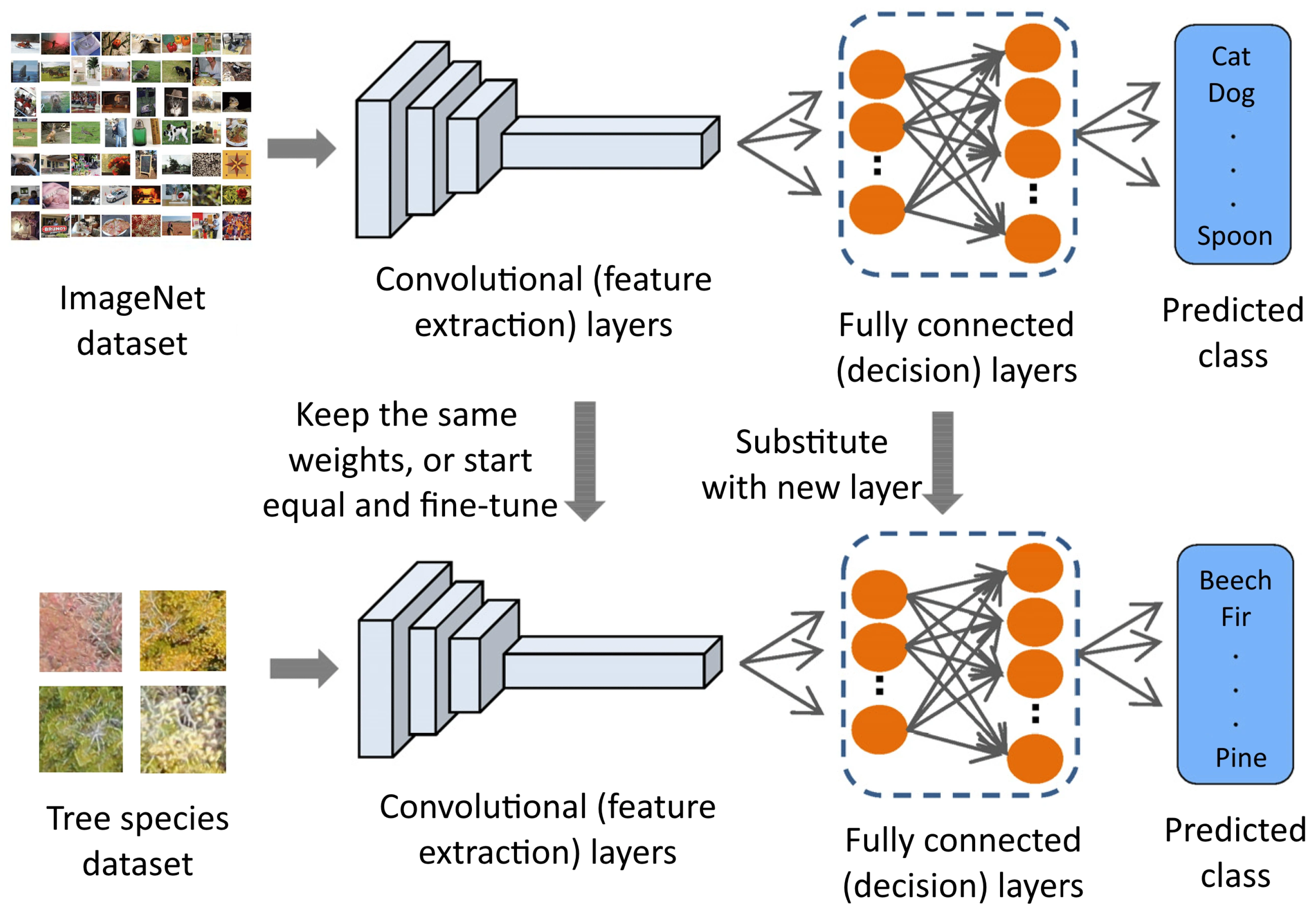
Transfer Learning
Setup for Finding the Best Model
Setup for Data-Quantity Test
Setup for Use-Case Test
2.2.2. Biodiversity Estimation
- Species Richness () [44], which stands for the number of different species represented in an ecological community.
- The Shannon–Wiener Index () [45], which stands for the uncertainty in predicting the species identity of an individual that is taken at random from the dataset. Higher values of this index thus represent higher biodiversity. See Equation (1):where is the ratio of trees of species i within the dataset: , with number of individuals of species i. Values between 1.5 and 3.5 are commonly considered as “high biodiversity”.
- The Gini–Simpson Index () [46], which is known in ecology as the probability of inter-specific encounters or the probability that two random trees in the dataset have different species. See Equation (2):This value ranges from 0 to 1, with higher values (closer to 1) representing higher biodiversity.
Setup for Biodiversity-Estimation Test
2.2.3. Evaluation Metrics
3. Results
3.1. Finding the Best Model
3.2. Data-Quantity Test
3.3. Biodiversity-Estimation Test
3.4. Use-Case Test
3.5. Hardware and Computational Time Considerations
4. Discussion
5. Conclusions
Author Contributions
Funding
Data Availability Statement
Acknowledgments
Conflicts of Interest
References
- Beck, P.S.; Atzberger, C.; Høgda, K.A.; Johansen, B.; Skidmore, A.K. Improved monitoring of vegetation dynamics at very high latitudes: A new method using MODIS NDVI. Remote. Sens. Environ. 2006, 100, 321–334. [Google Scholar] [CrossRef]
- Atkinson, P.M.; Jeganathan, C.; Dash, J.; Atzberger, C. Inter-comparison of four models for smoothing satellite sensor time-series data to estimate vegetation phenology. Remote. Sens. Environ. 2012, 123, 400–417. [Google Scholar] [CrossRef]
- Garioud, A.; Valero, S.; Giordano, S.; Mallet, C. Recurrent-based regression of Sentinel time series for continuous vegetation monitoring. Remote. Sens. Environ. 2021, 263, 112419. [Google Scholar] [CrossRef]
- Parisi, F.; Vangi, E.; Francini, S.; D’Amico, G.; Chirici, G.; Marchetti, M.; Lombardi, F.; Travaglini, D.; Ravera, S.; De Santis, E.; et al. Sentinel-2 time series analysis for monitoring multi-taxon biodiversity in mountain beech forests. Front. For. Glob. Chang. 2023, 6, 1020477. [Google Scholar] [CrossRef]
- Alterio, E.; Campagnaro, T.; Sallustio, L.; Burrascano, S.; Casella, L.; Sitzia, T. Forest management plans as data source for the assessment of the conservation status of European Union habitat types. Front. For. Glob. Chang. 2023, 5, 1069462. [Google Scholar] [CrossRef]
- Liu, X.; Frey, J.; Munteanu, C.; Still, N.; Koch, B. Mapping tree species diversity in temperate montane forests using Sentinel-1 and Sentinel-2 imagery and topography data. Remote. Sens. Environ. 2023, 292, 113576. [Google Scholar] [CrossRef]
- Rossi, C.; McMillan, N.A.; Schweizer, J.M.; Gholizadeh, H.; Groen, M.; Ioannidis, N.; Hauser, L.T. Parcel level temporal variance of remotely sensed spectral reflectance predicts plant diversity. Environ. Res. Lett. 2024, 19, 074023. [Google Scholar] [CrossRef]
- Madonsela, S.; Cho, M.A.; Ramoelo, A.; Mutanga, O.; Naidoo, L. Estimating tree species diversity in the savannah using NDVI and woody canopy cover. Int. J. Appl. Earth Obs. Geoinf. 2018, 66, 106–115. [Google Scholar] [CrossRef]
- Immitzer, M.; Neuwirth, M.; Böck, S.; Brenner, H.; Vuolo, F.; Atzberger, C. Optimal Input Features for Tree Species Classification in Central Europe Based on Multi-Temporal Sentinel-2 Data. Remote. Sens. 2019, 11, 2599. [Google Scholar] [CrossRef]
- Verrelst, J.; Halabuk, A.; Atzberger, C.; Hank, T.; Steinhauser, S.; Berger, K. A comprehensive survey on quantifying non-photosynthetic vegetation cover and biomass from imaging spectroscopy. Ecol. Indic. 2023, 155, 110911. [Google Scholar] [CrossRef]
- Lechner, M.; Dostálová, A.; Hollaus, M.; Atzberger, C.; Immitzer, M. Combination of Sentinel-1 and Sentinel-2 Data for Tree Species Classification in a Central European Biosphere Reserve. Remote. Sens. 2022, 14, 2687. [Google Scholar] [CrossRef]
- Yan, S.; Jing, L.; Wang, H. A New Individual Tree Species Recognition Method Based on a Convolutional Neural Network and High-Spatial Resolution Remote Sensing Imagery. Remote. Sens. 2021, 13, 479. [Google Scholar] [CrossRef]
- Wan, H.; Tang, Y.; Jing, L.; Li, H.; Qiu, F.; Wu, W. Tree Species Classification of Forest Stands Using Multisource Remote Sensing Data. Remote. Sens. 2021, 13, 144. [Google Scholar] [CrossRef]
- Iglseder, A.; Immitzer, M.; Dostálová, A.; Kasper, A.; Pfeifer, N.; Bauerhansl, C.; Schöttl, S.; Hollaus, M. The potential of combining satellite and airborne remote sensing data for habitat classification and monitoring in forest landscapes. Int. J. Appl. Earth Obs. Geoinf. 2023, 117, 103131. [Google Scholar] [CrossRef]
- Kattenborn, T.; Leitloff, J.; Schiefer, F.; Hinz, S. Review on Convolutional Neural Networks (CNN) in vegetation remote sensing. ISPRS J. Photogramm. Remote. Sens. 2021, 173, 24–49. [Google Scholar] [CrossRef]
- Diez, Y.; Kentsch, S.; Fukuda, M.; Caceres, M.L.L.; Moritake, K.; Cabezas, M. Deep Learning in Forestry Using UAV-Acquired RGB Data: A Practical Review. Remote. Sens. 2021, 13, 2837. [Google Scholar] [CrossRef]
- Egli, S.; Höpke, M. CNN-Based Tree Species Classification Using High Resolution RGB Image Data from Automated UAV Observations. Remote. Sens. 2020, 12, 3892. [Google Scholar] [CrossRef]
- Kentsch, S.; Cabezas, M.; Tomhave, L.; Groß, J.; Burkhard, B.; Lopez Caceres, M.L.; Waki, K.; Diez, Y. Analysis of UAV-Acquired Wetland Orthomosaics Using GIS, Computer Vision, Computational Topology and Deep Learning. Sensors 2021, 21, 471. [Google Scholar] [CrossRef]
- Cabezas, M.; Kentsch, S.; Tomhave, L.; Gross, J.; Caceres, M.L.L.; Diez, Y. Detection of Invasive Species in Wetlands: Practical DL with Heavily Imbalanced Data. Remote. Sens. 2020, 12, 3431. [Google Scholar] [CrossRef]
- Dash, J.P.; Watt, M.S.; Pearse, G.D.; Heaphy, M.; Dungey, H.S. Assessing very high resolution UAV imagery for monitoring forest health during a simulated disease outbreak. ISPRS J. Photogramm. Remote. Sens. 2017, 131, 1–14. [Google Scholar] [CrossRef]
- Safonova, A.; Tabik, S.; Alcaraz-Segura, D.; Rubtsov, A.; Maglinets, Y.; Herrera, F. Detection of fir trees (Abies sibirica) damaged by the bark beetle in unmanned aerial vehicle images with deep learning. Remote. Sens. 2019, 11, 643. [Google Scholar] [CrossRef]
- Nguyen, H.T.; Lopez Caceres, M.L.; Moritake, K.; Kentsch, S.; Shu, H.; Diez, Y. Individual Sick Fir Tree (Abies mariesii) Identification in Insect Infested Forests by Means of UAV Images and Deep Learning. Remote. Sens. 2021, 13, 260. [Google Scholar] [CrossRef]
- Moritake, K.; Cabezas, M.; Nhung, T.T.C.; Lopez Caceres, M.L.; Diez, Y. Sub-alpine shrub classification using UAV images: Performance of human observers vs. DL classifiers. Ecol. Inform. 2024, 80, 102462. [Google Scholar] [CrossRef]
- Zhang, C.; Atkinson, P.M.; George, C.; Wen, Z.; Diazgranados, M.; Gerard, F. Identifying and mapping individual plants in a highly diverse high-elevation ecosystem using UAV imagery and deep learning. ISPRS J. Photogramm. Remote. Sens. 2020, 169, 280–291. [Google Scholar] [CrossRef]
- Sun, Y.; Huang, J.; Ao, Z.; Lao, D.; Xin, Q. Deep Learning Approaches for the Mapping of Tree Species Diversity in a Tropical Wetland Using Airborne LiDAR and High-Spatial-Resolution Remote Sensing Images. Forests 2019, 10, 1047. [Google Scholar] [CrossRef]
- Sylvain, J.D.; Drolet, G.; Brown, N. Mapping dead forest cover using a deep convolutional neural network and digital aerial photography. ISPRS J. Photogramm. Remote. Sens. 2019, 156, 14–26. [Google Scholar] [CrossRef]
- Agisoft LLC. Agisoft Metashape. Available online: https://www.agisoft.com/ (accessed on 15 September 2024).
- O’shea, K.; Nash, R. An introduction to convolutional neural networks. arXiv 2015, arXiv:1511.08458. [Google Scholar]
- Vaswani, A.; Shazeer, N.; Parmar, N.; Uszkoreit, J.; Jones, L.; Gomez, A.N.; Kaiser, Ł.; Polosukhin, I. Attention is all you need. Adv. Neural Inf. Process. Syst. 2017, 30, 5999–6009. [Google Scholar]
- Deng, J.; Dong, W.; Socher, R.; Li, L.J.; Li, K.; Li, F.-F. ImageNet: A large-scale hierarchical image database. In Proceedings of the 2009 IEEE Conference on Computer Vision and Pattern Recognition, Miami, FL, USA, 20–25 June 2009; pp. 248–255. [Google Scholar] [CrossRef]
- He, K.; Zhang, X.; Ren, S.; Sun, J. Deep residual learning for image recognition. In Proceedings of the IEEE/CVF Conference on Computer Vision and Pattern Recognition (CVPR), Las Vegas, NV, USA, 27–30 June 2016; pp. 770–778. [Google Scholar]
- Radosavovic, I.; Kosaraju, R.P.; Girshick, R.; He, K.; Dollár, P. Designing network design spaces. In Proceedings of the IEEE/CVF Conference on Computer Vision and Pattern Recognition (CVPR), Seattle, WA, USA, 13–19 June 2020; pp. 10428–10436. [Google Scholar]
- Liu, Z.; Mao, H.; Wu, C.Y.; Feichtenhofer, C.; Darrell, T.; Xie, S. A ConvNet for the 2020s. In Proceedings of the IEEE/CVF Conference on Computer Vision and Pattern Recognition (CVPR), New Orleans, LA, USA, 18–24 June 2022; pp. 11976–11986. [Google Scholar]
- Liu, Z.; Lin, Y.; Cao, Y.; Hu, H.; Wei, Y.; Zhang, Z.; Lin, S.; Guo, B. Swin Transformer: Hierarchical Vision Transformer Using Shifted Windows. In Proceedings of the IEEE/CVF International Conference on Computer Vision (ICCV), Montreal, BC, Canada, 11–17 October 2021; pp. 10012–10022. [Google Scholar]
- Liu, Z.; Hu, H.; Lin, Y.; Yao, Z.; Xie, Z.; Wei, Y.; Ning, J.; Cao, Y.; Zhang, Z.; Dong, L.; et al. Swin Transformer V2: Scaling up Capacity and Resolution. In Proceedings of the IEEE/CVF Conference on Computer Vision and Pattern Recognition (CVPR), New Orleans, LA, USA, 18–24 June 2022; pp. 12009–12019. [Google Scholar]
- Leidemer, T.; Gonroudobou, O.B.H.; Nguyen, H.T.; Ferracini, C.; Burkhard, B.; Diez, Y.; Lopez Caceres, M.L. Classifying the Degree of Bark Beetle-Induced Damage on Fir (Abies mariesii) Forests, from UAV-Acquired RGB Images. Computation 2022, 10, 63. [Google Scholar] [CrossRef]
- Xie, Y.; Ling, J. Wood defect classification based on lightweight convolutional neural networks. BioResources 2023, 18, 7663–7680. [Google Scholar] [CrossRef]
- Schiefer, F.; Kattenborn, T.; Frick, A.; Frey, J.; Schall, P.; Koch, B.; Schmidtlein, S. Mapping forest tree species in high resolution UAV-based RGB-imagery by means of convolutional neural networks. ISPRS J. Photogramm. Remote. Sens. 2020, 170, 205–215. [Google Scholar] [CrossRef]
- West, J.; Ventura, D.; Warnick, S. Spring Research Presentation: A Theoretical Foundation for Inductive Transfer; Brigham Young University, College of Physical and Mathematical Sciences: Provo, UT, USA, 2007; Volume 1. [Google Scholar]
- Bozinovski, S. Reminder of the first paper on transfer learning in neural networks, 1976. Informatica 2020, 44, 291–302. [Google Scholar] [CrossRef]
- Kentsch, S.; Lopez Caceres, M.L.; Serrano, D.; Roure, F.; Diez, Y. Computer Vision and Deep Learning Techniques for the Analysis of Drone-Acquired Forest Images, a Transfer Learning Study. Remote. Sens. 2020, 12, 1287. [Google Scholar] [CrossRef]
- Quinn, J.; McEachen, J.; Fullan, M.; Gardner, M.; Drummy, M. Dive into Deep Learning: Tools for Engagement; Corwin Press: Thousand Oaks, CA, USA, 2019. [Google Scholar]
- Mukhlif, A.A.; Al-Khateeb, B.; Mohammed, M.A. Incorporating a novel dual transfer learning approach for medical images. Sensors 2023, 23, 570. [Google Scholar] [CrossRef]
- Colwell, R.K., III. Biodiversity: Concepts, Patterns, and Measurement. In The Princeton Guide to Ecology; Princeton University Press: Princeton, NJ, USA, 2009; Chapter 3.1; pp. 257–263. [Google Scholar] [CrossRef]
- Spellerberg, I.F.; Fedor, P.J. A tribute to Claude Shannon (1916–2001) and a plea for more rigorous use of species richness, species diversity and the ‘Shannon–Wiener’ Index. Glob. Ecol. Biogeogr. 2003, 12, 177–179. [Google Scholar] [CrossRef]
- Breiman, L. Classification and Regression Trees; Routledge: London, UK, 2017. [Google Scholar]
- Powers, D. Evaluation: From Precision, Recall and F-Factor to ROC, Informedness, Markedness & Correlation. Mach. Learn. Technol. 2008, 2, 37–63. [Google Scholar]
- Sasaki, Y. The truth of the F-measure. Teach Tutor Mater 2007, 1, 5. [Google Scholar]
- Ting, K.M. Confusion Matrix. In Encyclopedia of Machine Learning and Data Mining; Sammut, C., Webb, G.I., Eds.; Springer: Boston, MA, USA, 2017; p. 260. [Google Scholar] [CrossRef]
- Bisong, E. Google Colaboratory. In Building Machine Learning and Deep Learning Models on Google Cloud Platform: A Comprehensive Guide for Beginners; Chapter Google Colaboratory; Apress: Berkeley, CA, USA, 2019; pp. 59–64. [Google Scholar] [CrossRef]
- Bolyn, C.; Lejeune, P.; Michez, A.; Latte, N. Mapping tree species proportions from satellite imagery using spectral–spatial deep learning. Remote. Sens. Environ. 2022, 280, 113205. [Google Scholar] [CrossRef]
- Shirai, H.; Kageyama, Y.; Nagamoto, D.; Kanamori, Y.; Tokunaga, N.; Kojima, T.; Akisawa, M. Detection method for Convallaria keiskei colonies in Hokkaido, Japan, by combining CNN and FCM using UAV-based remote sensing data. Ecol. Inform. 2022, 69, 101649. [Google Scholar] [CrossRef]
- Shirai, H.; Tung, N.D.M.; Kageyama, Y.; Ishizawa, C.; Nagamoto, D.; Abe, K.; Kojima, T.; Akisawa, M. Estimation of the Number of Convallaria Keiskei’s Colonies Using UAV Images Based on a Convolutional Neural Network. IEEJ Trans. Electr. Electron. Eng. 2020, 15, 1552–1554. [Google Scholar] [CrossRef]


| Species | Site 1 | Site 2 | Site 3 | Site 5 | Total per Species |
|---|---|---|---|---|---|
| Buna | 1489 | 202 | 1691 | ||
| Matsu | 7 | 97 | 104 | ||
| Minekaede | 16 | 185 | 1099 | 1300 | |
| Fir | 339 | 3182 | 3521 | ||
| Nanakamado | 195 | 355 | 346 | 896 | |
| Kyaraboku | 98 | 181 | 279 | ||
| Inutsuge | 119 | 71 | 190 | ||
| Mizuki | 84 | 231 | 315 | ||
| Koshiabura | 165 | 122 | 287 |
| Metric | RegNet | ConvNext | ResNet | Swin | |
|---|---|---|---|---|---|
| Accuracy | mean | 0.980 | 0.990 | 0.980 | 0.990 |
| std | 0.005 | 0.006 | 0.006 | 0.005 | |
| ci | (0.976, 0.984) | (0.986, 0.995) | (0.975, 0.984) | (0.987, 0.994) | |
| Precision | mean | 0.927 | 0.967 | 0.944 | 0.969 |
| std | 0.045 | 0.037 | 0.025 | 0.028 | |
| ci | (0.894, 0.959) | (0.941, 0.994) | (0.926, 0.962) | (0.949, 0.989) | |
| Recall | mean | 0.889 | 0.963 | 0.894 | 0.962 |
| std | 0.040 | 0.037 | 0.035 | 0.029 | |
| ci | (0.860, 0.917) | (0.937, 0.989) | (0.869, 0.919) | (0.941, 0.982) | |
| F1 Score | mean | 0.901 | 0.963 | 0.910 | 0.964 |
| std | 0.040 | 0.033 | 0.029 | 0.027 | |
| ci | (0.873, 0.930) | (0.939, 0.987) | (0.889, 0.931) | (0.945, 0.983) | |
| Architecture | Accuracy | Precision | Recall | F1 Score |
|---|---|---|---|---|
| RegNet | 97.85% | 96.66% | 92.38% | 94.02% |
| ConvNext | 99.22% | 96.58% | 98.90% | 97.64% |
| ResNet | 97.85% | 94.49% | 92.50% | 93.17% |
| Swin | 99.22% | 98.58% | 99.35% | 98.94% |
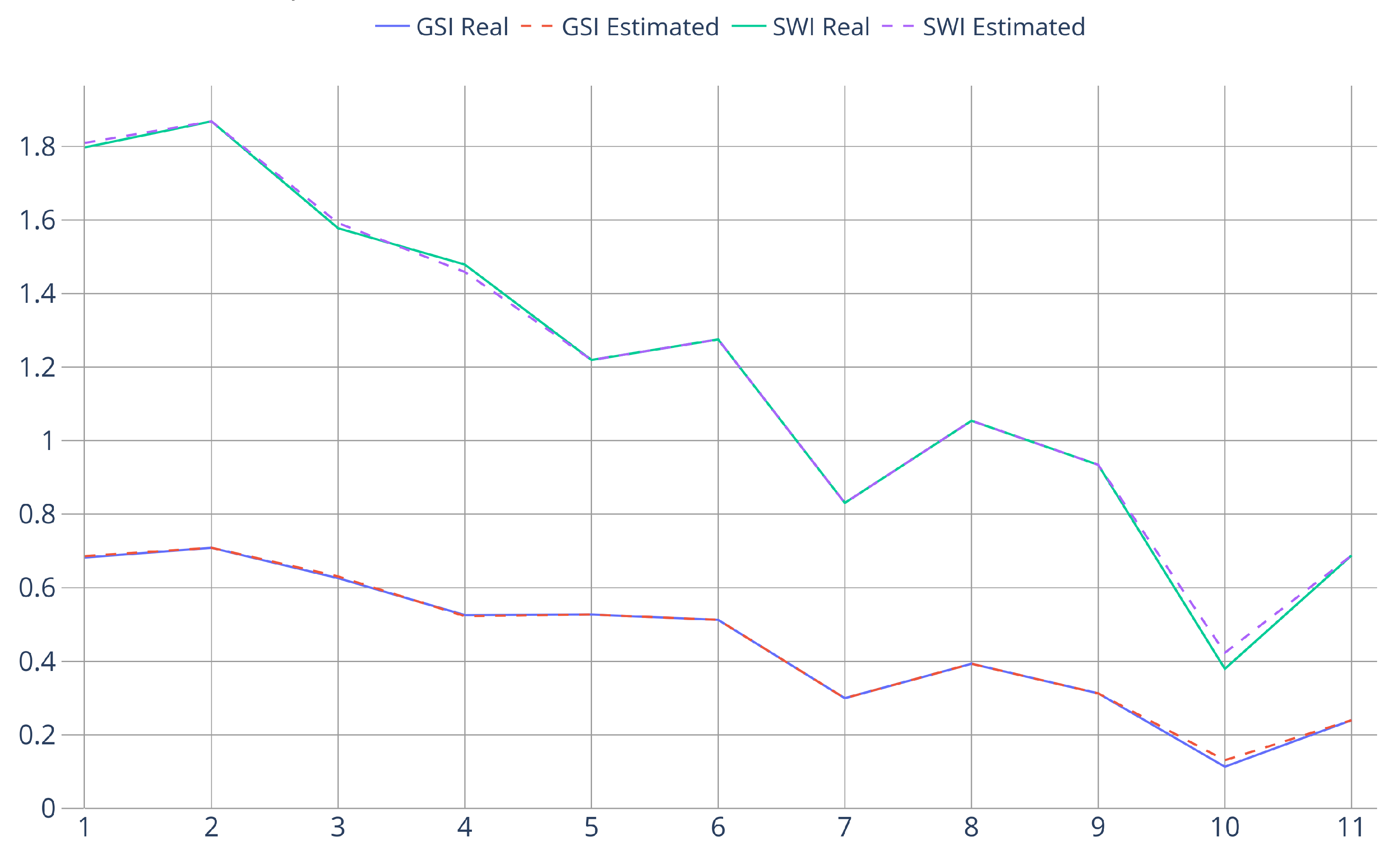
| Plot Number | Altitude [m] | Real Biodiversity | Estimated Biodiversity |
|---|---|---|---|
| 1 | 1337–1344 | : 4 : 0.6823 : 1.7973 | : 4 : 0.6862 : 1.7973 |
| 2 | 1350–1361 | : 4 : 0.7087 : 1.8682 | : 4 : 0.7087 : 1.8682 |
| 3 | 1367–1375 | : 4 : 0.6261 : 1.5774 | : 4 : 0.6307 : 1.5915 |
| 4 | 1397–1411 | : 5 : 0.5256 : 1.4789 | : 5 : 0.5228 : 1.4587 |
| 5 | 1403–1421 | : 4 : 0.5271 : 1.2193 | : 4 : 0.5271 : 1.2193 |
| 6 | 1390–1404 | : 3 : 0.5127 : 1.2752 | : 3 : 0.5127 : 1.2752 |
| 7 | 1407–1434 | : 3 : 0.2996 : 0.8306 | : 3 : 0.2996 : 0.8306 |
| 8 | 1414–1428 | : 4 : 0.3933 : 1.054 | : 4 : 0.3933 : 1.054 |
| 9 | 1435–1448 | : 4 : 0.3128 : 0.9343 | : 4 : 0.3128 : 0.9343 |
| 10 | 1454–1462 | : 3 : 0.1133 : 0.3796 | : 3 : 0.1310 : 0.4232 |
| 11 | 1464–1475 | : 3 : 0.2398 : 0.6877 | : 3 : 0.2398 : 0.6877 |
| VALIDATION | Fold 1 | Fold 2 | Fold 3 | Average | ||||
| Real | Pred | Real | Pred | Real | Pred | Real | Pred | |
| GSI | 0.6045 | 0.5991 | 0.8036 | 0.8051 | 0.6055 | 0.6054 | 0.6712 | 0.6699 |
| SWI | 2.0524 | 2.024 | 2.6556 | 2.6549 | 1.919 | 1.9214 | 2.209 | 2.2001 |
| SR | 9 | 9 | 8 | 8 | 8 | 8 | 8.67 | 8.67 |
| Acc | 96.85 | 98.5 | 98.14 | 97.83 | ||||
| F1 | 92.02 | 85.95 | 97.01 | 94.99 | ||||
| TEST | Fold 1 | Fold 2 | Fold 3 | Average | ||||
| Real | Pred | Real | Pred | Real | Pred | Real | Pred | |
| GSI | 0.6116 | 0.6455 | 0.453 | 0.482 | 0.6721 | 0.7296 | 0.5789 | 0.619 |
| SWI | 1.677 | 1.8939 | 1.5522 | 1.6326 | 1.7812 | 2.1997 | 1.6701 | 1.9087 |
| SR | 5 | 7 | 8 | 9 | 4 | 8 | 5.67 | 8 |
| Acc | 95.56 | 92.76 | 83.59 | 90.64 | ||||
| F1 | 49.53 | 68.56 | 37.21 | 51.77 | ||||
| Name | Asus Zenbook UX535LH | Sedatech MS-7E07 |
| Processor | Intel Core i7-10870H 2.20 GHz | Intel Core i9-13900KF 3.00 GHz |
| Graphics card | NVIDIA GeForce GTX 1650 Max-Q 4 GB | NVIDIA GeForce RTX 4090 24 GB |
| RAM | 16 GB DDR4 | 128 GB DDR5 |
| Data preprocessing and augmentation time (full dataset) | 21 min | 3 min and 36 s |
| Training time (full dataset) | 16 h and 42 min | 1 h and 8 min |
| Inference time (100 images) | 2.123 s | 0.735 s |
Disclaimer/Publisher’s Note: The statements, opinions and data contained in all publications are solely those of the individual author(s) and contributor(s) and not of MDPI and/or the editor(s). MDPI and/or the editor(s) disclaim responsibility for any injury to people or property resulting from any ideas, methods, instructions or products referred to in the content. |
© 2024 by the authors. Licensee MDPI, Basel, Switzerland. This article is an open access article distributed under the terms and conditions of the Creative Commons Attribution (CC BY) license (https://creativecommons.org/licenses/by/4.0/).
Share and Cite
Conciatori, M.; Tran, N.T.C.; Diez, Y.; Valletta, A.; Segalini, A.; Lopez Caceres, M.L. Plant Species Classification and Biodiversity Estimation from UAV Images with Deep Learning. Remote Sens. 2024, 16, 3654. https://doi.org/10.3390/rs16193654
Conciatori M, Tran NTC, Diez Y, Valletta A, Segalini A, Lopez Caceres ML. Plant Species Classification and Biodiversity Estimation from UAV Images with Deep Learning. Remote Sensing. 2024; 16(19):3654. https://doi.org/10.3390/rs16193654
Chicago/Turabian StyleConciatori, Marco, Nhung Thi Cam Tran, Yago Diez, Alessandro Valletta, Andrea Segalini, and Maximo Larry Lopez Caceres. 2024. "Plant Species Classification and Biodiversity Estimation from UAV Images with Deep Learning" Remote Sensing 16, no. 19: 3654. https://doi.org/10.3390/rs16193654
APA StyleConciatori, M., Tran, N. T. C., Diez, Y., Valletta, A., Segalini, A., & Lopez Caceres, M. L. (2024). Plant Species Classification and Biodiversity Estimation from UAV Images with Deep Learning. Remote Sensing, 16(19), 3654. https://doi.org/10.3390/rs16193654