Abstract
Thin clouds in Remote Sensing (RS) imagery can negatively impact subsequent applications. Current Deep Learning (DL) approaches often prioritize information recovery in cloud-covered areas but may not adequately preserve information in cloud-free regions, leading to color distortion, detail loss, and visual artifacts. This study proposes a Sparse Transformer-based Generative Adversarial Network (SpT-GAN) to solve these problems. First, a global enhancement feature extraction module is added to the generator’s top layer to enhance the model’s ability to preserve ground feature information in cloud-free areas. Then, the processed feature map is reconstructed using the sparse transformer-based encoder and decoder with an adaptive threshold filtering mechanism to ensure sparsity. This mechanism enables that the model preserves robust long-range modeling capabilities while disregarding irrelevant details. In addition, inverted residual Fourier transformation blocks are added at each level of the structure to filter redundant information and enhance the quality of the generated cloud-free images. Finally, a composite loss function is created to minimize error in the generated images, resulting in improved resolution and color fidelity. SpT-GAN achieves outstanding results in removing clouds both quantitatively and visually, with Structural Similarity Index (SSIM) values of 98.06% and 92.19% and Peak Signal-to-Noise Ratio (PSNR) values of 36.19 dB and 30.53 dB on the RICE1 and T-Cloud datasets, respectively. On the T-Cloud dataset, especially with more complex cloud components, the superior ability of SpT-GAN to restore ground details is more evident.
1. Introduction
Significant progress has been made in the technology of earth observation satellites, especially with optical Remote Sensing (RS) imagery. This technology has been extensively used in various industries, such as agricultural management, urban planning, environmental monitoring, and resource prospecting. According to the International Satellite Cloud Climatology Project, the average annual cloud cover worldwide is as high as 66% [1,2]. In practical applications, a significant portion of RS imagery is often obscured by clouds and fog, leading to loss of information, blurred details, and color distortion in the obscured areas, resulting in reduced reliability. This limitation adversely impacts a range of downstream tasks, such as target detection [3], land cover change monitoring [4], and land cover classification [5], hindering their effectiveness and reliability in practical applications.
Thick cloud cover may obstruct all surface information, making it challenging to achieve satisfactory results using a single RS image for cloud removal and limiting its research value. Thin clouds, characterized by their lower optical thickness and limited impact on overall RS images compared to thicker clouds, permit partial sunlight transmission and allow partial surface information to reach satellite sensors [6]. This feature facilitates data recovery from areas obscured by thin cloud cover using only a single image. As a result, eliminating thin cloud cover from individual RS images is a significant task when preprocessing RS imagery.
Substantial achievements have been made in reconstructing images affected by thin clouds and haze pollution using both Deep Learning (DL)-based and traditional conventional image processing techniques. Traditional methods have been extensively used in previous studies due to their simplicity and interpretability. Many traditional image processing approaches treat thin clouds as low-frequency components [7,8,9] in the frequency domain, processing the low-frequency information of images to reduce or eliminate the impact of thin clouds and haze in images by enhancing surface features. For instance, Hu et al. [10] presented a thin cloud removal technique based on the dual-tree complex wavelet transform to remove clouds through sub-band decomposition and low-frequency coefficient prediction. Imaging models have been utilized to understand the formation of images in optical systems, and have been extensively applied to remove thin clouds from RS images [11,12,13]. Sahu et al. [14] proposed a method that divides the image into blocks, selects the block with the highest score to estimate the atmospheric light, and eliminates atmospheric scattering through novel color channels, then employed illumination scaling factors to improve the dehazed image. He et al. [15] introduced the Dark Channel Prior (DCP) algorithm in 2010, which estimates the atmospheric light component and transmittance in cloudy images based on an atmospheric scattering model for removing thin clouds and haze. Many methods are derived from DCP for thin cloud and haze removal [16,17,18]. Image filtering techniques are also widely employed for thin cloud and haze removal [19,20]. The Homomorphic Filtering (HF) method proposed by Peli et al. [21] is a commonly used approach; the image is first converted from the spatial domain to the frequency domain, then integrated with the atmospheric scattering model to remove thin clouds and haze by compressing brightness and enhancing contrast. Although traditional image processing methods can successfully remove clouds under certain conditions, they rely on specific physical assumptions and mathematical models which may not fully reflect the real-world situation, leading to difficulties in accurately restoring the accurate ground information.
With the recent development of DL technology, numerous studies have developed various models for removing clouds and haze that are tailored to the characteristics of optical RS images. Unlike traditional methods, DL approaches can adaptively learn and optimize, providing advantages when handling complex scenes. Furthermore, these approaches can generate cloud-free images that are more realistic and exhibit finer details. Zhang et al. [22] proposed a unified spatiotemporal spectral framework based on Convolutional Neural Networks (CNNs) to eliminate clouds using multisource data for unified processing. Li et al. [23] introduced an end-to-end Residual Symmetric Cascaded Network (RSC-Net), which employs symmetrical convolutional–deconvolutional concatenations to better preserve the detail in declouded images. Zhou et al. [24] proposed a multiscale attention residual network for thin cloud removal which combined large-scale filters and fine-grained convolution residual blocks to enhance feature extraction. Ding et al. [25] presented a Conditional Variational Auto-Encoder (CVAE) with uncertainty analysis to produce multiple plausible cloud-free pictures for each multicloud image. Zi et al. [26] proposed a wavelet integral convolutional neural network, integrating wavelet inverse transform into the encoder–decoder architecture for thin cloud removal. Guo et al. [27] introduced Cloud Perception Integrated Fast Fourier Convolutional Network (CP-FFCN), a single image-based blind method for thin cloud removal. CP-FFCN employs a cloud perception module and a fast Fourier convolution reconstruction module to effectively model and remove clouds in RS images without requiring external knowledge of cloud distribution. GANs are widely applied in RS images to remove clouds because they effectively generate realistic and diverse images [28,29,30]. Wang et al. [31] improved the structural similarity index of cloud-free images by introducing a novel objective function in their conditional GAN for cloud removal. Li et al. [32] removed thin clouds by integrating cloud distortion physical models into a GAN. Tan et al. [33] presented a contrastive learning-based unsupervised RS technique called GAN-UD for removing thin clouds from images.
While current DL-based methods can successfully remove thin clouds from RS images characterized by relatively simple structures such as clear delineation between cloud and land features and limited atmospheric interference, they struggle when the clouds vary in thickness or shape. These methods often struggle to achieve high-quality restoration in areas with uneven cloud cover, leading to detail loss and blurring. Most existing approaches focus primarily on recovering information from cloud-covered regions, which can result in over-correction in areas with thin clouds, causing artifacts and edge distortion. Additionally, architectural limitations in current models may lead to color deviations compared to actual surface information, even after successful cloud removal; such discrepancies and uneven restoration not only degrade image quality but also hinder downstream tasks sensitive to color variations, such as land cover classification and quantitative analyses.
This study introduces an end-to-end network based on a sparse transformer that leverages a multi-head self-attention mechanism, which we name Sparse Transformer-based Generative Adversarial Network (SpT-GAN). This study effectively models complex long-range dependencies and ignores irrelevant information, considering the excellent long-range modeling capability of the multi-head self-attention [34] for capturing relationships between pixels in images. This mechanism enhances the model’s information restoration for areas covered by thin clouds. In addition, this study introduces a Global Enhancement Feature Extraction (GEFE) module designed to take advantage of partial ground detail information that can penetrate through thin clouds to reach sensors on satellites. This module enhances the model’s ability to preserve ground information in cloud-free and sparsely cloud-covered areas. The proposed method makes the following contributions:
- 1.
- We introduce a sparse multi-head self-attention (sparse attention) module to build the transformer block within the generator. This module utilizes the self-attention mechanism’s outstanding long-range modeling capabilities to model global pixel relationships, enhancing the model’s ability to reconstruct cloud-free images. It employs a weight-learnable filtering mechanism to retain information from highly relevant areas while neglecting information from low-correlation areas.
- 2.
- Moreover, we propose a GEFE module to capture aggregated features from different directions and enhance the model’s extraction of perceivable surface information.
- 3.
- Our study demonstrates that the proposed SpT-GAN effectively removes clouds for both uniform and nonuniform thin cloud RS images across various scenes without significantly increasing computational complexity. Experimental results on public datasets, including RICE1 and T-Cloud, show that the generated images exhibit precise details, high color fidelity, and close resemblance to the authentic ground images.
The rest of this paper is organized as follows: Section 2 provides a brief introduction to related work; Section 3 thoroughly explains the proposed approach; Section 4 presents the dataset specifics, analysis, experimental results, and relevant discussion; finally, Section 5 presents our conclusions.
2. Related Works
In this part, a brief introduction to the existing attention mechanism-based cloud removal methods is provided in Section 2.1, while Section 2.2 briefly introduces different transformers applied to DL tasks.
2.1. Attention-Mechanism-Based Cloud Removal Methods
Attention mechanisms play a critical role in improving the performance and efficiency of models when dealing with long sequences and complex tasks. In RS image cloud removal, integrating attention mechanisms can help models to effectively focus on and process critical information in the image, thereby enhancing the accuracy and efficiency of cloud removal tasks. For instance, attention mechanisms allow models to selectively enhance relevant areas while minimizing the impact of extraneous noise in remote sensing images originating from sources such as sensor noise, atmospheric interference, and background clutter. Several RS cloud removal models rely on attention mechanisms [35,36,37]. Moreover, spatial attention is widely used in cloud removal [28,38,39], as it emphasizes the arrangement and structure of inputs in space. Several methods also incorporate self-attention to achieve cloud removal [40,41]. In addition, a number of methods use different combinations of attention to achieve cloud removal. For instance, Liu et al. [42] proposed Semantic Information-Structural Attention Generative Adversarial Network (SI-SA GAN), which combines spatial attention with self-attention to remove clouds. Ding et al. [43] proposed the Contextual Residual Fusion Block Network (CRFB-Net), which integrates spatial and channel attention. Jin et al. [44] presented the Hybrid Attention Generative Adversarial Network (HyA-GAN), which combines channel and spatial attention mechanisms to prioritize important regions in images and remove clouds.
Many methods for removing thin clouds prioritize cloud-covered areas and disregard cloud-free regions on the ground surface. This issue emerges due to the way in which ordinary attention mechanisms primarily enable the model to differentiate between clouds and underlying features, which results in a lack of focus on preserving details in cloud-free regions. This paper proposes SpT-GAN, which combines two different attention mechanisms to address this issue and enhance the features of cloudy and cloud-free areas in order to achieve effective cloud removal. First, the GEFE module based on coordinate attention enhances details in cloud-free areas. This framework is followed by sparse attention in the sparse transformer block, which focuses on processing cloud-covered areas. These two strategies complement each other and help the model to recover details across all image regions.
2.2. Transformers in Deep Learning Tasks
The transformer self-attention mechanism was first introduced in [34], revolutionizing sequence modeling in natural language processing. Self-attention enhances the ability to capture long-range dependencies and facilitates parallelization during training [45], significantly improving efficiency. As a result, transformers have become the foundation for state-of-the-art models, driving advancements in tasks such as Computer Vision (CV) [46,47,48], speech recognition [49,50], and time series prediction [51,52] with advanced DL technologies. One type of CV task is cloud removal in RS imagery. Below, we discuss several typical transformers used in CV tasks. For instance, Zamir et al. [46] proposed an encoder–decoder transformer called Restormer for image restoration. Restormer utilizes self-attention mechanisms in both the encoder and decoder stages to capture long-range dependencies. Dosovitskiy et al. [53] incorporated Vision Transformer (ViT), which applies a standard transformer directly to sequences of image patches for image classification. Han et al. [54] presented the transformer-in-transformer model, which enhances the representation capability of ViT by incorporating inner-patch transformers within the main transformer framework. Wu et al. [40] introduced a transformer-based network called Cloudformer which effectively combines convolution and self-attention mechanisms with locally-enhanced positional encoding to enhance cloud removal in optical RS images. Yun et al. [55] proposed Single-Head Vision Transformer (SHViT), which optimizes speed and accuracy for image classification and object detection.
The sparse transformer approach [56] effectively manages long-range dependencies and improves computational efficiency [57] by introducing a sparse attention mechanism. Chen et al. [58] introduced an optimization of ViT called SparseViT that involves activating sparse regions based on their importance and using evolutionary search to determine optimal layer-wise pruning ratios. Huang et al. [59] proposed a U-Net style transformer-based network called Spa-former for image in-painting. This network addresses computational challenges while improving long-range feature modeling, resulting in superior performance.
In this study, the generator of our proposed SpT-GAN adopts a U-Net-style transformer-based network. It incorporates a skip connection to improve long-range dependency modeling and integrates sparsity into the multi-head self-attention mechanism to mitigate excessive attention towards noise and irrelevant information.
3. Methodology
We introduce the SpT-GAN method employing a transformer module with sparse attention and the GEFE module to construct the generator for our GAN, with the goal of effectively eliminating thin clouds from remote sensing images. First, the overall structure of SpT-GAN is introduced in Section 3.1. Then, the GEFE module is described in Section 3.2. Subsequently, the specific structure and the implementation principle of the transformer block are elaborated in Section 3.3. Finally, Section 3.4 introduces the composite loss function.
3.1. Overview of the Proposed Framework
The proposed model architecture consists of a sparse transformer-based generator and a discriminator. The generator is responsible for producing fake cloud-free images, which are then fed into the discriminator for parameter optimization. The optimization procedure of the generator and discriminator forms a min–max optimization problem [60]. When the generator and discriminator each reach their optimal states relative to their respective minimum and maximum values, it indicates that the generator has successfully captured the feature distribution of the real cloud-free images. Through this procedure, the GAN enables the model to generate more realistic cloud-free images. In this study, the generator adopts a U-Net structure and the discriminator is derived from Patch-GAN [61]. Details about the specific structures of the generator and discriminator are illustrated in Figure 1a and Figure 1b, respectively.
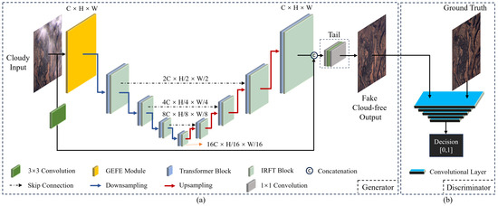
Figure 1.
Overview of SpT-GAN: (a) U-Net-based generator and (b) Patch-GAN-based discriminator.
3.1.1. Generator
In Figure 1a, the raw cloud-containing image is separately fed as input into the GEFE module and a convolution block. The GEFE module enhances ground surface features within the cloudy image, while the convolution block incorporates reflection padding to maintain image integrity. Subsequently, the feature map produced by the GEFE module is downsampled and fed into the first transformer block for feature extraction. After this block, an Inverted Residual Fourier Transformation (IRFT block) block [62] refines the feature information by utilizing the Fast Fourier Transform (FFT), which converts spatial features into the frequency domain, effectively separating high-frequency details from low-frequency components to aid in the identification and emphasis of important features while filtering out noise. Each encoder consists of a downsampling operation followed by a Transformer–IRFT layer. Following that, the feature map produced by the first encoder undergoes identical operations, persisting until the procedure concludes with the fourth encoder. In this process, the size of the feature map changes from to , aiding the model in extracting more complex features from the cloudy images.
The decoding process is followed by progressive upsampling to restore the feature map to the cloud image’s original size and level of detail. The decoder is similar to the encoder, except that it replaces downsampling operations with upsampling operations. In the final stage of the decoding phase, the generated feature map is combined with the original image processed by the convolution block, resulting in a concatenated feature map with a size of . Introducing skip connections helps to integrate richer feature information, enhancing the model’s ability to reconstruct declouded images and restore surface details. Finally, the concatenated image passes through a tail module comprising three convolutional layers for reconstruction, restoring the image size to and obtaining a cloud-free image.
3.1.2. Discriminator
Figure 1b shows the discriminator, which comprises five convolutional layers. The first four layers incorporate downsampling, convolution, and activation functions. These procedures enable accurate differentiation between actual and fake cloud-free image pairs by extracting features from each pair. Initially, the fake–real cloud-free image pairs are combined and fed into the first convolutional layer, where the concatenated images undergo downsampling through convolution operations, with the introduction of nonlinearity via the Leaky ReLU activation function. The convolutional operations in the second to the fourth layers are similar to those in the first layer, except that batch normalization is added before the activation function to enhance network stability. The fifth convolutional layer consists solely of a convolutional operation and a sigmoid activation function, producing an output value between 0 and 1. A value approaching 1 indicates that the generated fake images are more likely to be considered authentic; conversely, a lower value suggests that the generated fake images exhibit more significant differences from the real ones. Utilizing this mechanism, the discriminator provides feedback to the generator, iteratively improving the generator’s performance.
3.2. Global Enhancement Feature Extraction Module
This subsection develops the GEFE module. As depicted in Figure 2a, this module comprises a Coordinate Attention [63] Feature Extraction block (CAFE block) fused with an IRFT block. The coordinate attention mechanism is illustrated in Figure 2b. The IRFT block incorporates inverted residual blocks (iR blocks) from MobileNetV2 [64] to help the model perceive surface details of RS imagery while utilizing lower computational resources. To address the practical scenario of a batch size of 1, we have replaced the batch normalization originally used in coordinate attention with instance normalization [65], as batch normalization is unsuitable for processing small batch data [66]. The GEFE module assigns learnable attention weights to feature channels, enabling the model to leverage salient features from multiple levels of RS images. By emphasizing ground-level detail information while suppressing irrelevant details, the module effectively captures ground-level detail information in cloud-free regions, enhancing the model’s capacity to extract surface information.
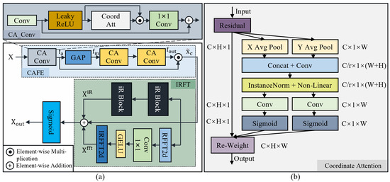
Figure 2.
(a) Illustration of the GEFE module and (b) illustration of the coordinate attention mechanism.
In the illustration of the GEFE module, the input cloud-containing image X is first processed by the CAFE block to compute the attention weights, highlighting essential regions within the cloud image. The resulting weighted feature map is input to the IRFT block to enhance the details, improving image clarity and detail representation capability. Finally, a sigmoid activation function is applied for nonlinear activation to help the module learn better cloud-free feature representations, resulting in a new feature map .
The CAFE block is used to apply attention-weighting operations on cloud-containing images, which helps to preserve important information on the ground surface. Initially, the input X is fed into the first coordinate attention convolution (CA_Conv) block, generating the feature map , where C represents the channel dimension and H and W respectively denote the height and width of the input image. Then, the output feature map is generated by applying the Global Average Pooling (GAP) operation as the channel descriptor to leverage the rich features. Following this, attention weights are computed through two CA_Conv blocks with convolution kernel sizes of , resulting in a new feature map denoted as . In the figure, CA_Conv blocks with different colors indicate the use of different-sized convolution kernels. Finally, the output representation denoted by is obtained by multiplying with :
The CA_Conv block within the CAFE module uses the following workflow: first, the input image undergoes convolution through the initial convolutional layer, where the kernel size of this convolutional layer can be adjusted according to the task requirements; second, the output of the convolutional layer is activated using the Leaky ReLU activation function with a negative slope of 0.2; third, feature weighting is conducted through the coordinate attention mechanism, multiplying the weighted features by the activated features, with a kernel size convolutional layer deployed for additional convolutional processes; finally, the weighted features are added to the original features to produce the final output . The mathematical expression for this module is as follows:
where X denotes the original input, represents the convolution operation, represents the coordinate attention mechanism, indicates the Leaky ReLU activation function, and ⊙ signifies element-wise multiplication.
3.3. Sparse Transformer Block
In RS imagery, removing thin clouds is critical for repairing the image. Inspired by the Spa-former [59] method used for image restoration, we developed a sparse transformer block to efficiently remove thin clouds and produce high-quality cloud-free images. This method effectively models remote dependencies with linear complexity, making it suitable for RS imagery with complex surface features. The transformer block comprises sparse attention and Feed-Forward Network (FFN) modules. Figure 3a and Figure 3b respectively depict the structures of the sparse attention and FFN modules.
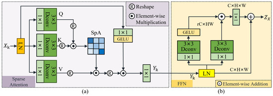
Figure 3.
(a) Illustration of the sparse attention module and (b) illustration of the FFN module.
3.3.1. Sparse Attention
The long-range modeling capabilities of the sparse transformer module significantly improve inference performance in areas with severe information loss during cloud removal operations in RS imagery. The module’s core is the sparse attention module, depicted in Figure 3a, which comprises Layer Normalization (LN), gated operations, and sparse multi-head self-attention. The LN is applied to the input features to stabilize the input feature distribution. After processing feature distribution, it is input to the sparse attention layer. In this layer, the attention maps from each head are computed and concatenated after computation to obtain the attention result . In addition, a spatial gating mechanism is introduced to guide the attention results for spatial features. A spatial gating mechanism is also introduced to obtain gating values for each spatial position through a convolution and a GELU activation function. The values are used to introduce an element-wise product operation with the attention result , obtaining the feature result . Finally, the feature result is processed through a convolution to obtain the final output. In summary, the function of the k-th sparse attention module is as follows:
where is the feature map input to the sparse attention module, represents the module’s output, denotes the layer normalization, is the sparse attention, indicates the GELU activation function, and ⊙ is the element-wise multiplication.
We incorporate a filtering mechanism into the multi-head self-attention module to suppress low-relevance features which might contain noise or irrelevant information. This mechanism introduces sparsity by selectively attending to high-relevance features, thereby enhancing the focus of the attention heads on crucial details and improving the overall model’s performance and efficiency. The filtering mechanism is shown in Figure 4.

Figure 4.
Illustration of the filtering mechanism.
First, we segment the original attention feature map into n attention heads, resulting in segmented attention feature maps . Next, we compute attention weights and pass them through the GELU activation function. The activated weights of each attention head are then transferred to a filter in which a learnable threshold is applied; the initial value of is set to . During training, the threshold adaptively adjusts its value based on the optimizer to ensure the reliability of the sparse attention module. If any value in the weight matrix of the feature map is less than , its weight is set to 0. The filtered outputs form new feature maps, which are eventually concatenated to generate the final attention feature map . The proposed sparsity strategy can be mathematically expressed as follows:
where is the attention result; the query , key , and value are computed from input features , where is the resolution of the input feature; H, W, and C are the height, width, and channel of the input feature, respectively; D is the inner dimension of the embedding feature; the attention map is ; is a transformation function, which requires each value to ensure the definition of the correlation in attention map A; and denotes the filtering mechanism with learnable threshold .
3.3.2. Feed-Forward Network
Figure 3b shows that the FFN is comprised of the LN and gating operations along with a residual connection [67]. The gating operation first expands the feature map channel from C to on two branches, where r is an expansion factor. In the left branch, the processed feature map undergoes convolution operations to blend features after passing through the LN operation. Subsequently, the GELU activation function enhances nonlinear representation; this approach is widely used in the FFN structure of transformer models thanks to its ability to mitigate gradient vanishing and provide more stable training. The function of the feature map at this stage is as follows:
where is the feature map input to the FFN module and consists of a convolution and a depth-wise convolution.
The right branch is similar to the left, except that it excludes the GELU activation function. At the end of the FFN module, a residual connection is added between the input and gated feature maps. The function of the FFN in the k-th transformer block is denoted as follows:
where is the output of the FFN module and consists of a convolution and a depth-wise convolution.
3.4. Loss Function
In this work, we build a composite loss function aimed at minimizing the disparity between the generated cloud-free images and actual cloud-free photographs. The composite loss function includes the reconstruction loss [68], adversarial loss [69], perceptual loss [70], and edge loss [71]. These loss functions constrain the model from several angles and improve both the quality and authenticity of the generated cloud-free images, making them similar to authentic cloud-free images. These loss functions complement each other by considering various features. By allowing for the comprehensive consideration of different features, the composite loss function endows the model with more robust generalization capabilities. The mathematical expression for the loss function is as follows:
where , , and are the weight parameters, which were carefully optimized through experimentation to achieve the optimal balance between the substituent loss functions. After extensive testing, the best balance for this task was determined to be , , .
The reconstruction loss quantifies the disparity between the generated cloud-free image and the original cloud-free image. By optimizing the pixel-level -norm distance, the model can more effectively restore detailed information in the areas of the image hidden by thin clouds. The reconstruction loss is represented mathematically as follows:
where and respectively represent the created cloud-free image and the original cloud-free image, while denotes the -norm, which quantifies the discrepancy between and .
The adversarial loss incorporates adversarial training to evaluate the authenticity of the generated cloud-free image, which offers insights into improving the image’s realism and help to bring the image closer to the corresponding ground truth. The adversarial loss is represented mathematically as follows:
where is the discriminator used in the model, denotes the expectation operation concerning the original cloud-free image , and denotes the expectation operation with respect to the created cloud-free image .
The perceptual loss is used to evaluate the consistency between real images obtained by a pretrained VGG19 network [72] and the restored images. The main objective is to minimize , or the distance between high-level features, which improves the model’s ability to restore the semantic information of the actual ground surface. This mechanism aims to generate cloud-free images that accurately reproduce the form, texture, and structural characteristics of surface objects. The mathematical representation of the perceptual loss is as follows:
Finally, the edge loss serves to guide the model’s attention toward image details. In RS pictures, thin cloud layers frequently mask ground objects’ fine detail and texture. By introducing the edge loss, the generated cloud-free images can more closely approximate the real ground surface images at the edges, allowing for better preservation of ground objects’ boundary and contour information. Its mathematical representation is as follows:
where represents the Laplacian operator used for edge detection in images.
4. Results and Analysis
The experimental settings are discussed in Section 4.1, including descriptions of the implementation details, datasets, and evaluation metrics. Section 4.2 compares our results with other methods. Section 4.3 discusses model complexity, while Section 4.4 presents the results and analysis of ablation experiments. Finally, Section 4.5 validates the robustness of SpT-GAN by processing the output cloud-free images.
4.1. Experimental Settings
4.1.1. Implementation Details
The proposed model was built using the PyTorch framework. The computational platform included an Intel(R) Xeon(R) Silver 4310 CPU and an Nvidia A100 GPU with 80 GB of RAM. During training, the proposed model was optimized using the AdamW optimizer [73], which features adaptive learning rate characteristics. The initial parameters included , , a weight decay of 0.00001, a batch size of 1, 300 training epochs, eight attention heads, and an initial learning rate of 0.0004.
4.1.2. Description of Datasets
We evaluated the proposed model using the RICE1 [74] and T-Cloud [25] datasets. A comparison between the RICE1 dataset and the T-Cloud dataset is shown in Table 1, while samples from both datasets are shown in Figure 5.

Table 1.
Comparison between the RICE1 and T-Cloud datasets.
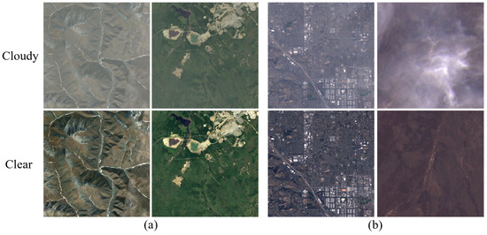
Figure 5.
Dataset samples: (a) RICE1 dataset and (b) T-Cloud dataset.
The RICE1 dataset comprises 500 pairs of cloud-covered images and corresponding cloud-free images extracted from Google Earth, each with a resolution of pixels; the image acquisition period is 15 days. Most of the cloud-covered images in this dataset exhibit relatively uniform cloud formations.
By contrast, the T-Cloud dataset consists of 2939 pairs of cloud-covered images and corresponding cloud-free images captured by Landsat-8, each with a resolution of pixels. The images in each pair are taken 16 days apart due to the satellite re-entry period. The cloud formations in the T-Cloud dataset are more complex, featuring uneven cloud distribution and varying thicknesses. Both datasets comprise natural-color images collected from diverse ground scenes, including urban areas, mountainous regions, and coastlines.
Experimental assessments were conducted to evaluate the proposed model’s generalization capabilities across these two datasets with diverse cloud formations. For each of the RICE1 and T-Cloud datasets, of the images were used for training and the remaining were used for testing.
4.1.3. Evaluation Metrics
The experimental results were evaluated using three quantitative evaluation metrics: Peak Signal to Noise Ratio (PSNR) [75], Structural Similarity Index (SSIM) [76], and Learned Perceptual Image Patch Similarity (LPIPS) [77]. These three evaluation metrics depend on comparing results with a reference image to highlight the relative performance of each method. We utilized real cloud-free images from the dataset as reference images to ensure a fair comparison of the differences among the methods. PSNR measures the difference between images at the pixel level based on error sensitivity, SSIM assesses the similarity between the reconstructed and reference images, and LPIPS aligns more closely with human perception. Higher PSNR and SSIM values indicate better quality of the generated images, while lower LPIPS values suggest that the generated image is more perceptibly similar to the real image. The mathematical definition of PSNR is as follows:
where n is the number of bits per pixel, H and W respectively stand for the height and width of the image, and is the mean squared error between the ground truth and the fake image .
The mathematical definition of SSIM is as follows:
where represents the similarity in luminance, indicates the contrast similarity, represents the structural similarity, is a weighting parameter, and are the respective mean brightness values of images and , and are the respective brightness variances of images and , the covariance of the luminance between images and is represented by , and , , and are constants utilized to prevent division by 0.
The mathematical definition of LPIPS is as follows:
where represents the distance between X and , , and respectively indicate the height, width, and weight of the l-th layer, and signify the features predicted by the model and baseline, respectively, at position , and ⊙ stands for element-wise multiplication.
4.2. Comparison with Other Methods
This section employs two different types of methods for quantitative analysis, namely, hypothesis-driven approaches and deep learning methods. The hypothesis-driven approach selects the representative DCP [15] method, while the DL methods include McGAN [78], SpA-GAN [28], AMGAN-CR [79], CVAE [25], MSDA-CR [80], and MemoryNet [81].
(1) Quantitative results analysis: The quantitative comparison of experiments on the RICE1 and T-Cloud datasets shown in Table 2 indicates that SpT-GAN achieves better PSNR, SSIM, and LPIPS values than the other methods. DCP shows relatively lower performance on both datasets, likely due to its more basic approach. Methods such as McGAN and SpA-GAN demonstrate strong performance on RICE1 but exhibit variability on T-Cloud, highlighting their sensitivity to dataset characteristics. In contrast, AMGAN-CR encounters similar challenges while showing better performance on the T-Cloud dataset. While CVAE and MSDA-CR achieve notable results in terms of specific metrics, they do not match the overall effectiveness of SpT-GAN across both datasets. Compared to MemoryNet, which is the most recent best method, SpT-GAN shows respective improvements of 1.83 dB and 0.98 dB in PSNR, 0.33% and 0.76% in SSIM, and 0.0032 and 0.0095 in LPIPS on the RICE1 and T-Cloud datasets. This comprehensive analysis leads to the conclusion that our method holds a decisive advantage in restoring true surface information, which is thanks to the powerful long-range modeling ability of sparse attention and the excellent global detail perception ability of the GEFE module.
Table 2.
Quantitative results on the RICE1 and T-Cloud datasets. The ↑ symbol indicates that larger values are better, while ↓ indicates that smaller values are better.
Figure 6 presents the box plots of the MSE results for each DL-based method across two datasets. The box plots illustrate performance differences, with a thicker box positioned higher and many outliers typically indicating larger errors and poorer performance. In contrast, a lower and narrower box with a more concentrated distribution of outliers suggests better performance. The box plot results generated by these methods are highly correlated with the data presented in Table 2, and the generalization ability and performance differences of various methods across different datasets can be clearly observed. The MSE results of SpT-GAN on both datasets demonstrate its stable performance and good generalization capability.

Figure 6.
Box plots of the MSE results produced by each DL-based method: (a) RICE1 dataset and (b) T-Cloud dataset.
(2) Qualitative result analysis of DL-based methods on the RICE1 dataset: Upon visual comparison of the results presented in Figure 7, it can be observed that the McGAN method can effectively remove uniformly distributed thin clouds but struggles with images containing unevenly distributed thin clouds, resulting in detail loss and artifacts. The thin cloud removal results generated by SpA-GAN exhibit satisfactory overall performance, although some color distortion is present. The thin cloud removal results generated by SpA-GAN and McGAN are generally satisfactory, reflecting effective learning of data distribution through their GAN-based architectures. However, both models’ relatively simple generator structures lead to the aforementioned adverse results. AMGAN-CR produces images with advanced color saturation and contrast; however, it suffers from artifact issues in some images, impacting the overall visual quality. The MemoryNet method successfully removes the thin clouds in all scenes, albeit with an overall increase in the brightness in the generated images. AMGAN-CR and MemoryNet cause brightness enhancement, which may be due to their inability to accurately model the true distribution of image brightness. The results of CVAE demonstrate that while the thin clouds are effectively removed, the resulting images still exhibit some color distortions and the model does not perform as expected on images containing unevenly distributed thin clouds, indicating inferior generalization ability in handling such variations. In addition, the images generated by MSDA-CR exhibit color differences in some scenes compared to the real cloud-free images.
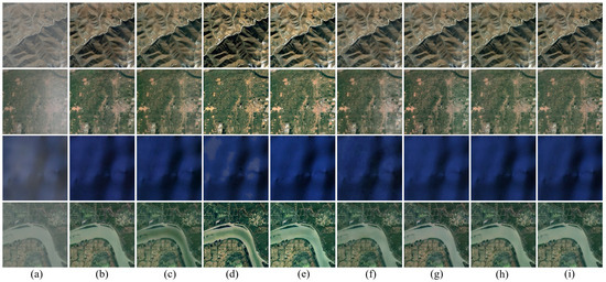
Figure 7.
Results of DL-based methods on the RICE1 dataset: (a) cloudy images, (b) McGAN [78], (c) SpA-GAN [28], (d) AMGAN-CR [79], (e) MemoryNet [81], (f) CVAE [25], (g) MSDA-CR [80], (h) our proposed method, (i) cloud-free images.
Figure 8 illustrates the zoomed-in details of the cloud-free images generated by each DL-based method. Upon observing the enlarged details, it is apparent that the details and edges produced by the AMGAN-CR method appear unnatural, with an increase in contrast. Both CVAE and MSDA-CR fail to eliminate thin clouds in the highlighted areas. The detailed representations generated by McGAN and SpA-GAN are insufficiently precise, making it challenging to interpret real surface information accurately. In addition, the images generated by MemoryNet are brighter than the ground truth image. By contrast, SpT-GAN completely removes the thin clouds in the highlighted regions and provides visual fidelity closer to real surface conditions.

Figure 8.
Magnified details of the results of each DL-method on the RICE1 dataset: (a) cloudy images, (b) McGAN [78], (c) SpA-GAN [28], (d) AMGAN-CR [79], (e) MemoryNet [81], (f) CVAE [25], (g) MSDA-CR [80], (h) our proposed method, (i) cloud-free images.
(3) Qualitative result analysis of DL-based methods on the T-Cloud dataset: Figure 9 depicts the overall visual effects of each technique on the T-Cloud dataset. This dataset contains various forms of thin clouds, making it particularly challenging to assess the performance of models. Visual inspection shows that McGAN, SpA-GAN, AMGAN-CR, and MSDA-CR can remove simple thin clouds but struggle with complex cloud formations, resulting in artifacts. The second cloud-free image generated by MemoryNet does not meet the expected level of cloud removal, resulting in an effect similar to haze cover. While CVAE demonstrates cloud removal effects that are generally close to expectations, tiny artifacts still appear in some images. Notably, SpT-GAN consistently produces the best visual results even under wide-area uneven cloud cover conditions.
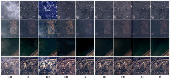
Figure 9.
Results of each DL-method on the T-Cloud dataset: (a) cloudy images, (b) McGAN [78], (c) SpA-GAN [28], (d) AMGAN-CR [79], (e) MemoryNet [81], (f) CVAE [25], (g) MSDA-CR [80], (h) our proposed method, (i) cloud-free images.
Figure 10 presents a detailed comparison of each method’s performance on the T-Cloud dataset. Only SpT-GAN achieves the optimal level of detail. Other methods, including SpA-GAN, AMGAN-CR, and CVAE, are not utterly successful in removing the cloud regions outlined in the boxes. These results may stem from the attention mechanisms employed by these methods, which could cause them to overly concentrate on cloud-covered areas and neglect global image features. Isolating cloud-covered areas during processing may inadvertently amplify artifacts or inconsistencies in the unaffected regions of the image. The insufficient integration of local and global features could result in incomplete or inaccurate restoration of the underlying surface, thereby degrading the overall quality of the output, preventing these models from extracting effective features and leading to their failing to remove clouds. MSDA-CR and MemoryNet successfully remove clouds, but reduce the image’s overall brightness, making it challenging to interpret details. Although McGAN removes the clouds, its information recovery of cloud-covered surfaces is not as effective as SpT-GAN.
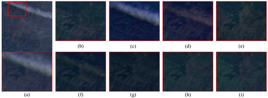
Figure 10.
Magnified details of the results of each DL-method on the T-Cloud dataset: (a) cloudy images, (b) McGAN [78], (c) SpA-GAN [28], (d) AMGAN-CR [79], (e) MemoryNet [81], (f) CVAE [25], (g) MSDA-CR [80], (h) our proposed method, (i) cloud-free images.
Based on these findings, it can be concluded that SpT-GAN exhibits excellent performance in cloud removal and ground detail restoration, even for datasets such as T-Cloud that contain complex cloud shapes.
4.3. Model Complexity Evaluation
We performed comparative experimental evaluations of the complexity of the various DL models, aiming to explore the correlation between model complexity and the efficacy of cloud removal. We used the T-Cloud dataset to validate the inference speed in Frames Per Second (FPS) of each model in practical applications, while all other metrics were tested using the shape tensors . A comparison of complexity metrics for each model is presented in Table 3.
Table 3.
Comparison of the computational complexity of each DL-based method.
The model’s complexity is comprehensively reflected through the parameter count, computational complexity, and model size metrics. Here, FPS denotes the speed at which the model processes data, the parameter count refers to the number of changeable parameters in the model that require learning and optimization, the computational complexity indicates the amount of floating-point operations, representing the number of multiplications and additions required during model execution, and the model size represents the storage space occupied by the pretrained parameters generated after training the model. Compared with other methods, SpT-GAN effectively removes thin clouds with a relatively lower parameter count and computational complexity. Specifically, SpT-GAN has 5.85 M parameters, which is significantly fewer than McGAN and CVAE, although more than the other models. The Flops metric highlights the tradeoff between computational efficiency and task performance, with the results indicating that SpT-GAN effectively balances these factors. Although SpA-GAN has the lowest Flops and parameter count, it is less effective in cloud removal. SpT-GAN outperforms methods such as AMGAN-CR and CVAE in terms of efficiency. MemoryNet demands significantly more computation than the other models.
In summary, the proposed model effectively removes thin clouds with a relatively lower parameter count and computational complexity than other models. However, its inference speed does not correspondingly improve due to its low computational complexity, primarily due to its incorporation of a significant amount of depth-wise separable convolutions. One characteristic of depth-wise separable convolutions is their low computational complexity and high inference time [82]. Despite sacrificing a certain level of inference speed, the proposed model demonstrates relatively lower computational complexity and achieves superior cloud removal performance based on a comprehensive analysis of the experimental data.
4.4. Ablation Studies
We evaluated the impact of the IRFT block and the proposed GEFE module through ablation experiments assessing the impact of the loss function, number of attention heads, and sparsity strategy on the model’s cloud removal performance.
4.4.1. IRFT Block and GEFE Module Ablation Study
Table 4 displays the quantitative results for the IRFT block and the GEFE module. These experimental data indicate that including the IRFT block and GEFE module significantly improves the model’s performance. The difference in trainable parameter counts demonstrates that the IRFT module significantly increases the model’s parameter count; on the other hand, the GEFE module has a relatively minor impact on the number of parameters while still contributing positively to performance.
Table 4.
Quantitative results for the IRFT block and GEFE module. The ↑ symbol indicates that larger values are better, while ↓ indicates that smaller values are better.
Figure 11 shows the visual differences of the ablation experiment results. The roles of the GEFE and IRFT modules in the cloud removal task are evident from an examining the enlarged areas in the figure. Comparing Figure 11d–f, it is clear that the introduction of these two modules effectively reduces cloud artifacts in the generated images. The GEFE module focuses on surface information, enabling SpT-GAN to learn global features and mitigating the impact of clouds on image quality. On the other hand, the IRFT module employs FFT to treat the cloud-covered areas as low-frequency components in the frequency domain for filtering. Additionally, the GEFE module aids in aggregating global features, which helps to reduce color distortion in the generated images. The qualitative results presented in the figure are consistent with the quantitative results in Table 4, further confirming the significance of the GEFE and IRFT modules in the cloud removal task.
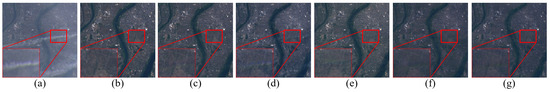
Figure 11.
Comparison showing the effectiveness of adding the IRFT block and GEFE module: (a) cloudy image, (b) ground truth, (c) complete SpT-GAN, (d) SpT-GAN without IRFT block and GEFE module, (e) SpT-GAN without IRFT block, (f) SpT-GAN without GEFE module, (g) SpT-GAN with the GEFE module replaced by a transformer block.
This section explores the attention weight allocation of the GEFE module, presenting experimental results through the attention heatmaps in Figure 12. From left to right, each set of images consists of a cloudy image, an attention heatmap generated by the GEFE module, and an attention heatmap generated by the transformer block. In the attention heatmaps, a higher intensity of red signifies the module’s greater allocation of attention weight to that particular region. In comparison, a lower intensity of color represents lower attention weight allocation. Observing the attention heatmaps generated by GEFE, it is evident that in Figure 12a most areas were obscured by cloud cover, rendering the surface information invisible; thus, the corresponding attention heatmaps are predominantly shaded in blue. In contrast to Figure 12b,d, areas not obstructed by clouds or covered by sufficiently sparse cloud layers are predominantly shaded in red, indicating the module’s capability to effectively filter out cloud contamination and focus on extracting surface information from sparsely cloud-covered and cloud-free regions, which is in alignment with the original design intent of the module. Substituting a transformer block for the GEFE module causes the model to focus primarily on cloud-covered areas. These results demonstrate that combining these two different attention mechanisms is essential for effectively removing clouds while enhancing the model’s ability to retain surface information.
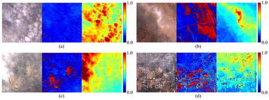
Figure 12.
Attention heatmaps of the GEFE module and the transformer block: (a) Extensive cloud coverage, (b) moderate cloud coverage, (c) uneven cloud coverage, (d) slight cloud coverage.
4.4.2. Loss Function Ablation Study
We performed additional ablation experiments using various combinations of loss functions to assess the impact of different loss functions on the declouding effect during optimization. The tested combinations included three control groups: one employing the classic GAN loss function combination of reconstruction loss and adversarial loss , a second incorporating the edge loss , and a third incorporating the perceptual loss . The experimental results are presented in Table 5.
Table 5.
Quantitative results for different loss functions. The ↑ symbol indicates that larger values are better, while ↓ indicates that smaller values are better.
As shown in Table 5, the data indicate that individually adding either the edge loss or perceptual loss contributes to the optimization of the model to a certain extent compared to the traditional GAN loss function combination . Notably, the effect of the perceptual loss was more pronounced for the RICE1 dataset, which has higher image resolution; however, the effect of the edge loss was comparatively more significant than for the T-Cloud dataset, which has lower image resolution. The final experimental results demonstrate that integrating all of these individual loss functions into a composite function yields the most favorable results, validating the effectiveness of the composite loss function constructed in this study.
4.4.3. Sparse Attention Ablation Study
The number of attention heads has an impact on the model’s performance. In the attention mechanism, multi-head attention allows the model to independently learn representations in different subspaces, thereby capturing more information and relationships. However, increasing the number of attention heads increases computational and memory requirements, which may lead to overfitting or reduced computational efficiency. When using the multi-head attention strategy, some attention heads may be redundant [83]. Therefore, we designed an experiment to investigate the influence of the attention heads and identify the optimal attention head strategy. In addition, this section presents experimental results on the impact of the sparsity strategy on model performance. The quantitative results with different numbers of heads and sparsity strategies are shown in Table 6.
Table 6.
Quantitative results for different numbers of heads and different sparsity strategies. The ↑ symbol indicates that larger values are better, while ↓ indicates that smaller values are better.
Upon analyzing the data presented in Table 6, it can be observed that a higher number of attention heads is not necessarily better; on the other hand, a reduced number of attention heads can result in the model being unable to fully capture the complex relationships and diversity of the input data, potentially leading to information loss. Due to the difference in resolution between the RICE1 and T-Cloud datasets, the influence of variations in attention head numbers exhibits diverse impacts on performance outcomes. Based on validation across these two experimental datasets, it was determined that eight attention heads are optimal for the proposed model.
Regarding sparsity strategies, the experimental data in Table 6 demonstrate that combining sparsity with varying numbers of attention heads can influence model performance to a certain extent. Moreover, introducing sparsity can reduce computational complexity. Our comprehensive analysis indicates that the sparse attention module effectively disregards some redundant information to enhance model performance.
4.5. Evaluation of Cloud-Free Image Processing
To further confirm the robustness of the proposed method, cloud-free images were used as inputs to the pretrained model for processing. Notably, the pretrained model was trained on datasets containing cloud-covered images, then was applied to process cloud-free images. The output results exhibited exceptional performance when compared with the original images in terms of both evaluation metrics and visual quality, indicating the model’s ability to effectively process images while disregarding cloud-related features. This observation underscores the high robustness of the proposed model. Visual comparisons are illustrated in Figure 13, the first row depicts the original cloud-free images and the second row displays the corresponding output results. This test holds significant practical relevance, as satellite sensors cannot consistently capture cloud-obscured images.
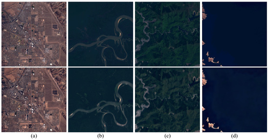
Figure 13.
Visual effect of cloudless image processing; the PSNR and SSIM values for each image pair are as follows: (a) PSNR 30.21 dB and SSIM 95.10%, (b) PSNR 33.67 dB and SSIM 98.04%, (c) PSNR 31.57 dB and SSIM 95.88%, (d) PSNR 29.37 dB and SSIM 97.21%.
5. Conclusions
This study proposes SpT-GAN, a novel method for removing thin clouds with different shapes and thicknesses while preserving high pixel-level similarity to real surface images. The proposed method employs a generator built upon an innovative sparse multi-head self-attention mechanism within the transformer block to adeptly model complex long-range dependencies. This advancement enhances the model’s capability to interpret RS images with intricate surface environments. The introduction of sparsity effectively filters out irrelevant information and enhances the quality of cloud-free images. In addition, we design a novel GEFE module to enhance the model’s ability to preserve surface details in cloud-free and sparse cloud areas. This module integrates a coordinate attention mechanism to enhance the model’s focus on surface details and an inverted residual Fourier transform block reduce redundant feature information. Compared to other DL-based approaches, the proposed model generates higher-quality cloud-free images and preserves surface details without significantly increasing computational complexity. Quantitative experimental results on two different datasets demonstrate the superiority of the proposed method. Furthermore, the proposed model does not perform cloud removal when processing cloud-free images and maintains high consistency with the original cloud-free images, indicating its good robustness.
Future research could extend the proposed model’s applicability by incorporating multi-band or synthetic aperture radar images. By combining techniques such as transfer learning, image fusion, and image transformation into the model, expanded data sources such as SAR and multispectral images would enable the model to gain a deeper understanding of thick cloud characteristics and acquire sufficient predictive experience to effectively reconstruct images contaminated by thick clouds. Considering the inference speed challenges of SpT-GAN, future research efforts could also explore ways of developing more efficient attention mechanisms to enhance the model’s inference speed while maintaining the effectiveness of cloud removal, potentially enabling direct deployment onto lightweight devices in the future.
Author Contributions
Conceptualization, J.H., X.G. and Y.Z. (Yinghui Zhao); methodology, J.H.; formal analysis, J.H., X.G., Y.Z. (Yinghui Zhao) and Y.Z. (Ying Zhou); investigation, J.H., X.G., Y.Z. (Yinghui Zhao) and Y.Z. (Ying Zhou); validation, J.H. and Y.Z. (Ying Zhou); resources, X.G. and Y.Z. (Yinghui Zhao); data curation, J.H.; writing—original draft preparation, J.H. and Y.Z. (Ying Zhou); writing—review and editing, J.H., X.G., Y.Z. (Yinghui Zhao) and Y.Z. (Ying Zhou); visualization, J.H.; supervision, X.G. and Y.Z. (Yinghui Zhao); project administration, X.G.; funding acquisition, X.G. All authors have read and agreed to the published version of the manuscript.
Funding
This research was funded by the Second Batch of the “Revealing the List and Appointing Leaders” Scientific and Technological Tackling of Projects in Heilongjiang Province (Grant No. 2021ZXJ05A01-04).
Data Availability Statement
The RICE dataset is available online at: https://github.com/BUPTLdy/RICE_DATASET (accessed on 19 June 2023). The T-Cloud dataset is available online at: https://github.com/haidong-Ding/Cloud-Removal (accessed on 13 September 2023).
Conflicts of Interest
The authors declare no conflicts of interest.
References
- Zhang, Y.; Rossow, W.B.; Lacis, A.A.; Oinas, V.; Mishchenko, M.I. Calculation of radiative fluxes from the surface to top of atmosphere based on ISCCP and other global data sets: Refinements of the radiative transfer model and the input data. J. Geophys. Res. Atmos. 2004, 109, D19. [Google Scholar] [CrossRef]
- King, M.D.; Platnick, S.; Menzel, W.P.; Ackerman, S.A.; Hubanks, P.A. Spatial and temporal distribution of clouds observed by MODIS onboard the Terra and Aqua satellites. IEEE Trans. Geosci. Remote Sens. 2013, 51, 3826–3852. [Google Scholar] [CrossRef]
- Hao, X.; Liu, L.; Yang, R.; Yin, L.; Zhang, L.; Li, X. A review of data augmentation methods of remote sensing image target recognition. Remote Sens. 2023, 15, 827. [Google Scholar] [CrossRef]
- Liu, C.; Li, W.; Zhu, G.; Zhou, H.; Yan, H.; Xue, P. Land use/land cover changes and their driving factors in the Northeastern Tibetan Plateau based on Geographical Detectors and Google Earth Engine: A case study in Gannan Prefecture. Remote Sens. 2020, 12, 3139. [Google Scholar] [CrossRef]
- Zhang, C.; Sargent, I.; Pan, X.; Li, H.; Gardiner, A.; Hare, J.; Atkinson, P.M. Joint Deep Learning for land cover and land use classification. Remote Sens. Environ. 2019, 221, 173–187. [Google Scholar] [CrossRef]
- Guo, J.; Yang, J.; Yue, H.; Tan, H.; Hou, C.; Li, K. RSDehazeNet: Dehazing network with channel refinement for multispectral remote sensing images. IEEE Trans. Geosci. Remote Sens. 2020, 59, 2535–2549. [Google Scholar] [CrossRef]
- Liu, Z.; Hunt, B.R. A new approach to removing cloud cover from satellite imagery. Comput. Vis. Graph. Image Process. 1984, 25, 252–256. [Google Scholar] [CrossRef]
- Shen, H.; Li, H.; Qian, Y.; Zhang, L.; Yuan, Q. An effective thin cloud removal procedure for visible remote sensing images. ISPRS J. Photogramm. Remote Sens. 2014, 96, 224–235. [Google Scholar] [CrossRef]
- Xu, M.; Jia, X.; Pickering, M.; Jia, S. Thin cloud removal from optical remote sensing images using the noise-adjusted principal components transform. ISPRS J. Photogramm. Remote Sens. 2019, 149, 215–225. [Google Scholar] [CrossRef]
- Hu, G.; Li, X.; Liang, D. Thin cloud removal from remote sensing images using multidirectional dual tree complex wavelet transform and transfer least square support vector regression. J. Appl. Remote Sens. 2015, 9, 095053. [Google Scholar] [CrossRef]
- Lv, H.; Wang, Y.; Shen, Y. An empirical and radiative transfer model based algorithm to remove thin clouds in visible bands. Remote Sens. Environ. 2016, 179, 183–195. [Google Scholar] [CrossRef]
- Zhou, B.; Wang, Y. A thin-cloud removal approach combining the cirrus band and RTM-based algorithm for Landsat-8 OLI data. In Proceedings of the 2019 IEEE International Geoscience and Remote Sensing Symposium (IGARSS), Yokohama, Japan, 28 July–2 August 2019; pp. 1434–1437. [Google Scholar]
- Song, C.; Xiao, C.; Zhang, Y.; Sui, H. Thin Cloud Removal for Single RGB Aerial Image. Comput Graph. Forum. 2021, 40, 398–409. [Google Scholar] [CrossRef]
- Sahu, G.; Seal, A.; Krejcar, O.; Yazidi, A. Single image dehazing using a new color channel. J. Vis. Commun. Image Represent. 2021, 74, 1–16. [Google Scholar] [CrossRef]
- He, K.; Sun, J.; Tang, X. Single image haze removal using dark channel prior. IEEE Trans. Pattern Anal. Mach. Intell. 2010, 33, 2341–2353. [Google Scholar]
- Liu, X.; Liu, C.; Lan, H.; Xie, L. Dehaze enhancement algorithm based on retinex theory for aerial images combined with dark channel. Open Access Libr. J. 2020, 7, 1–12. [Google Scholar] [CrossRef]
- Shi, S.; Zhang, Y.; Zhou, X.; Cheng, J. Cloud removal for single visible image based on modified dark channel prior with multiple scale. In Proceedings of the 2021 IEEE International Geoscience and Remote Sensing Symposium (IGARSS), Brussels, Belgium, 11–16 July 2021; pp. 4127–4130. [Google Scholar]
- Tang, Q.; Yang, J.; He, X.; Jia, W.; Zhang, Q.; Liu, H. Nighttime image dehazing based on Retinex and dark channel prior using Taylor series expansion. Comput. Vis. Image Underst. 2021, 202, 103086. [Google Scholar] [CrossRef]
- Han, Y.; Yin, M.; Duan, P.; Ghamisi, P. Edge-preserving filtering-based dehazing for remote sensing images. IEEE Geosci. Remote Sens. 2021, 19, 1–5. [Google Scholar] [CrossRef]
- Zhou, G.; He, L.; Qi, Y.; Yang, M.; Zhao, X.; Chao, Y. An improved algorithm using weighted guided coefficient and union self-adaptive image enhancement for single image haze removal. IET Image Process. 2021, 15, 2680–2692. [Google Scholar] [CrossRef]
- Peli, T.; Quatieri, T. Homomorphic restoration of images degraded by light cloud cover. In Proceedings of the 1984 IEEE International Conference on Acoustics, Speech, and Signal Processing (ICASSP), San Diego, CA, USA, 19–21 March 1984; pp. 100–103. [Google Scholar]
- Zhang, Q.; Yuan, Q.; Zeng, C.; Li, X.; Wei, Y. Missing data reconstruction in remote sensing image with a unified spatial–temporal–spectral deep convolutional neural network. IEEE Trans. Geosci. Remote Sens. 2018, 56, 4274–4288. [Google Scholar] [CrossRef]
- Li, W.; Li, Y.; Chen, D.; Chan, J.C.-W. Thin cloud removal with residual symmetrical concatenation network. ISPRS J. Photogramm. Remote Sens. 2019, 153, 137–150. [Google Scholar] [CrossRef]
- Zhou, Y.; Jing, W.; Wang, J.; Chen, G.; Scherer, R.; Damaševičius, R. MSAR-DefogNet: Lightweight cloud removal network for high resolution remote sensing images based on multi scale convolution. IET Image Process. 2022, 16, 659–668. [Google Scholar] [CrossRef]
- Ding, H.; Zi, Y.; Xie, F. Uncertainty-based thin cloud removal network via conditional variational autoencoders. In Proceedings of the 2022 Asian Conference on Computer Vision (ACCV), Macau SAR, China, 4–8 December 2022; pp. 469–485. [Google Scholar]
- Zi, Y.; Ding, H.; Xie, F.; Jiang, Z.; Song, X. Wavelet integrated convolutional neural network for thin cloud removal in remote sensing images. Remote Sens. 2023, 15, 781. [Google Scholar] [CrossRef]
- Guo, Y.; He, W.; Xia, Y.; Zhang, H. Blind single-image-based thin cloud removal using a cloud perception integrated fast Fourier convolutional network. ISPRS J. Photogramm. Remote Sens. 2023, 206, 63–86. [Google Scholar] [CrossRef]
- Pan, H. Cloud removal for remote sensing imagery via spatial attention generative adversarial network. arXiv 2020, arXiv:2009.13015. [Google Scholar]
- Huang, G.-L.; Wu, P.-Y. Ctgan: Cloud transformer generative adversarial network. In Proceedings of the 2022 IEEE International Conference on Image Processing (ICIP), Colombo, Sri Lanka, 16–19 October 2022; pp. 511–515. [Google Scholar]
- Ma, X.; Huang, Y.; Zhang, X.; Pun, M.-O.; Huang, B. Cloud-EGAN: Rethinking CycleGAN from a feature enhancement perspective for cloud removal by combining CNN and transformer. IEEE J. Sel. Top. Appl. Earth Obs. Remote Sens. 2023, 16, 4999–5012. [Google Scholar] [CrossRef]
- Wang, X.; Xu, G.; Wang, Y.; Lin, D.; Li, P.; Lin, X. Thin and thick cloud removal on remote sensing image by conditional generative adversarial network. In Proceedings of the 2019 IEEE International Geoscience and Remote Sensing Symposium(IGARSS), Yokohama, Japan, 28 July–2 August 2019; pp. 1426–1429. [Google Scholar]
- Li, J.; Wu, Z.; Hu, Z.; Zhang, J.; Li, M.; Mo, L.; Molinier, M. Thin cloud removal in optical remote sensing images based on generative adversarial networks and physical model of cloud distortion. ISPRS J. Photogramm. Remote Sens. 2020, 166, 373–389. [Google Scholar] [CrossRef]
- Tan, Z.C.; Du, X.F.; Man, W.; Xie, X.Z.; Wang, G.S.; Nie, Q. Unsupervised remote sensing image thin cloud removal method based on contrastive learning. IET Image Process. 2024, 18, 1844–1861. [Google Scholar] [CrossRef]
- Vaswani, A.; Shazeer, N.; Parmar, N.; Uszkoreit, J.; Jones, L.; Gomez, A.N.; Kaiser, Ł.; Polosukhin, I. Attention is all you need. In Advances in Neural Information Processing Systems; MIT Press: Cambridge, MA, USA, 2017; pp. 5998–6008. [Google Scholar]
- Wen, X.; Pan, Z.; Hu, Y.; Liu, J. An effective network integrating residual learning and channel attention mechanism for thin cloud removal. IEEE Geosci. Remote Sens. Lett. 2022, 19, 6507605. [Google Scholar] [CrossRef]
- Duan, C.; Li, R. Multi-head linear attention generative adversarial network for thin cloud removal. arXiv 2020, arXiv:2012.10898. [Google Scholar]
- Zou, X.; Li, K.; Xing, J.; Tao, P.; Cui, Y. PMAA: A progressive multi-scale attention autoencoder model for high-performance cloud removal from multi-temporal satellite imagery. arXiv 2023, arXiv:2303.16565. [Google Scholar]
- Chen, H.; Chen, R.; Li, N. Attentive generative adversarial network for removing thin cloud from a single remote sensing image. IET Image Process. 2021, 15, 856–867. [Google Scholar] [CrossRef]
- Jing, R.; Duan, F.; Lu, F.; Zhang, M.; Zhao, W. Cloud removal for optical remote sensing imagery using the SPA-CycleGAN network. J. Appl. Remote Sens. 2022, 16, 034520. [Google Scholar] [CrossRef]
- Wu, P.; Pan, Z.; Tang, H.; Hu, Y. Cloudformer: A cloud-removal network combining self-attention mechanism and convolution. Remote Sens. 2022, 14, 6132. [Google Scholar] [CrossRef]
- Zhao, B.; Zhou, J.; Xu, H.; Feng, X.; Sun, Y. PM-LSMN: A Physical-Model-based Lightweight Self-attention Multiscale Net For Thin Cloud Removal. Remote Sens. 2024, 21, 5003405. [Google Scholar] [CrossRef]
- Liu, J.; Hou, W.; Luo, X.; Su, J.; Hou, Y.; Wang, Z. SI-SA GAN: A generative adversarial network combined with spatial information and self-attention for removing thin cloud in optical remote sensing images. IEEE Access 2022, 10, 114318–114330. [Google Scholar] [CrossRef]
- Ding, H.; Xie, F.; Zi, Y.; Liao, W.; Song, X. Feedback network for compact thin cloud removal. IEEE Geosci. Remote Sens. Lett. 2023, 20, 6003505. [Google Scholar] [CrossRef]
- Jin, M.; Wang, P.; Li, Y. HyA-GAN: Remote sensing image cloud removal based on hybrid attention generation adversarial network. Int. J. Remote Sens. 2024, 45, 1755–1773. [Google Scholar] [CrossRef]
- Dufter, P.; Schmitt, M.; Schütze, H. Position information in transformers: An overview. Comput. Linguist. 2022, 48, 733–763. [Google Scholar] [CrossRef]
- Zamir, S.W.; Arora, A.; Khan, S.; Hayat, M.; Khan, F.S.; Yang, M.-H. Restormer: Efficient Transformer for High-Resolution Image Restoration. In Proceedings of the 2022 IEEE/CVF Conference on Computer Vision and Pattern Recognition (CVPR), New Orleans, LA, USA, 18–24 June 2022; pp. 5728–5739. [Google Scholar]
- Chen, X.; Li, H.; Li, M.; Pan, J. Learning A Sparse Transformer Network for Effective Image Deraining. In Proceedings of the 2023 IEEE/CVF Conference on Computer Vision and Pattern Recognition (CVPR), Vancouver, BC, Canada, 17–24 June 2023; pp. 5896–5905. [Google Scholar]
- Han, D.; Pan, X.; Han, Y.; Song, S.; Huang, G. Flatten transformer: Vision transformer using focused linear attention. In Proceedings of the 2023 IEEE/CVF International Conference on Computer Vision (ICCV), Paris, France, 2–6 October 2023; pp. 5961–5971. [Google Scholar]
- Kim, S.; Gholami, A.; Shaw, A.; Lee, N.; Mangalam, K.; Malik, J.; Mahoney, M.; Keutzer, K. Squeezeformer: An efficient transformer for automatic speech recognition. Adv. Neural Inf. Process. Syst. 2022, 35, 9361–9373. [Google Scholar]
- Chang, F.; Radfar, M.; Mouchtaris, A.; King, B.; Kunzmann, S. End-to-end multi-channel transformer for speech recognition. In Proceedings of the 2021 IEEE International Conference on Acoustics, Speech, and Signal Processing (ICASSP), Toronto, ON, Canada, 6–11 June 2021; pp. 5884–5888. [Google Scholar]
- Zhou, H.; Zhang, S.; Peng, J.; Zhang, S.; Li, J.; Xiong, H.; Zhang, W. Informer: Beyond efficient transformer for long sequence time-series forecasting. In Proceedings of the AAAI Conference on Artificial Intelligence, Virtual, 8–9 February 2021; Volume 35, pp. 11106–11115. [Google Scholar]
- Zhang, Y.; Yan, J. Crossformer: Transformer utilizing cross-dimension dependency for multivariate time series forecasting. In Proceedings of the Eleventh International Conference on Learning Representations (ICLR), Kigali, Rwanda, 1–5 May 2023. [Google Scholar]
- Dosovitskiy, A.; Beyer, L.; Kolesnikov, A.; Weissenborn, D.; Zhai, X.; Unterthiner, T.; Dehghani, M.; Minderer, M.; Heigold, G.; Gelly, S.; et al. An image is worth 16x16 words: Transformers for image recognition at scale. arXiv 2020, arXiv:2010.11929. [Google Scholar]
- Han, K.; Xiao, A.; Wu, E.; Guo, J.; Xu, C.; Wang, Y. Transformer in transformer. Adv. Neural Inf. Process. Syst. 2021, 34, 15908–15919. [Google Scholar]
- Yun, S.; Ro, Y. Shvit: Single-head vision transformer with memory efficient macro design. In Proceedings of the 2024 IEEE/CVF Conference on Computer Vision and Pattern Recognition (CVPR), Seattle WA, USA, 17–21 June 2024; pp. 5756–5767. [Google Scholar]
- Child, R.; Gray, S.; Radford, A.; Sutskever, I. Generating Long Sequences with Sparse Transformers. arXiv 2019, arXiv:1904.10509. [Google Scholar]
- Farina, M.; Ahmad, U.; Taha, A.; Younes, H.; Mesbah, Y.; Yu, X.; Pedrycz, W. Sparsity in Transformers: A Systematic Literature Review. Neurocomputing 2024, 582, 127468. [Google Scholar] [CrossRef]
- Chen, X.; Liu, Z.; Tang, H.; Yi, L.; Zhao, H.; Han, S. SparseViT: Revisiting Activation Sparsity for Efficient High-Resolution Vision Transformer. In Proceedings of the 2023 IEEE/CVF Conference on Computer Vision and Pattern Recognition (CVPR), Vancouver, BC, Canada, 17–24 June 2023; pp. 2061–2070. [Google Scholar]
- Huang, W.; Deng, Y.; Hui, S.; Wu, Y.; Zhou, S.; Wang, J. Sparse self-attention transformer for image inpainting. Pattern Recognit. 2024, 145, 109897. [Google Scholar] [CrossRef]
- Gui, J.; Sun, Z.; Wen, Y.; Tao, D.; Ye, J. A review on generative adversarial networks: Algorithms, theory, and applications. IEEE Trans. Knowl. Data Eng. 2021, 35, 3313–3332. [Google Scholar] [CrossRef]
- Isola, P.; Zhu, J.-Y.; Zhou, T.; Efros, A.A. Image-to-image translation with conditional adversarial networks. In Proceedings of the 2017 IEEE Conference on Computer Vision and Pattern Recognition (CVPR), Honolulu, HI, USA, 21–26 July 2017; pp. 1125–1134. [Google Scholar]
- Yae, S.; Ikehara, M. Inverted residual Fourier transformation for lightweight single image deblurring. IEEE Access 2023, 11, 29175–29182. [Google Scholar] [CrossRef]
- Hou, Q.; Zhou, D.; Feng, J. Coordinate attention for efficient mobile network design. In Proceedings of the 2021 IEEE/CVF Conference on Computer Vision and Pattern Recognition (CVPR), Nashville, TN, USA, 20–25 June 2021; pp. 13713–13722. [Google Scholar]
- Sandler, M.; Howard, A.; Zhu, M.; Zhmoginov, A.; Chen, L.-C. Mobilenetv2: Inverted residuals and linear bottlenecks. In Proceedings of the 2018 IEEE Conference on Computer Vision and Pattern Recognition (CVPR), Salt Lake City, UT, USA, 18–22 June 2018; pp. 4510–4520. [Google Scholar]
- Ulyanov, D.; Vedaldi, A.; Lempitsky, V. Instance normalization: The missing ingredient for fast stylization. arXiv 2016, arXiv:1607.08022. [Google Scholar]
- Huang, L.; Zhou, Y.; Wang, T.; Luo, J.; Liu, X. Delving into the estimation shift of batch normalization in a network. In Proceedings of the 2022 IEEE/CVF Conference on Computer Vision and Pattern Recognition (CVPR), New Orleans, LA, USA, 19–23 June 2022; pp. 763–772. [Google Scholar]
- Szegedy, C.; Ioffe, S.; Vanhoucke, V.; Alemi, A. Inception-v4, Inception-ResNet and the Impact of Residual Connections on Learning. In Proceedings of the AAAI Conference on Artificial Intelligence, San Francisco, CA, USA, 8–12 October 2016. [Google Scholar]
- Kingma, D.P.; Welling, M. Auto-encoding variational bayes. arXiv 2013, arXiv:1312.6114. [Google Scholar]
- Goodfellow, I.J.; Pouget-Abadie, J.; Mirza, M.; Xu, B.; Warde-Farley, D.; Ozair, S.; Courville, A.; Bengio, Y. Generative adversarial nets. In Proceedings of the International Conference on Neural Information Processing Systems (NIPS), Montreal, QC, Canada, 8–13 December 2014; pp. 2672–2680. [Google Scholar]
- Zhou, C.; Zhang, J.; Liu, J.; Zhang, C.; Fei, R.; Xu, S. PercepPan: Towards unsupervised pan-sharpening based on perceptual loss. Remote Sens. 2020, 12, 2318. [Google Scholar] [CrossRef]
- Niklaus, S.; Liu, F. Context-aware synthesis for video frame interpolation. In Proceedings of the IEEE Conference on Computer Vision and Pattern Recognition, Salt Lake City, UT, USA, 18–22 June 2018; pp. 1701–1710. [Google Scholar]
- Simonyan, K.; Zisserman, A. Very deep convolutional networks for large-scale image recognition. arXiv 2014, arXiv:1409.1556. [Google Scholar]
- Loshchilov, I.; Hutter, F. Decoupled weight decay regularization. arXiv 2017, arXiv:1711.05101. [Google Scholar]
- Lin, D.; Xu, G.; Wang, X.; Wang, Y.; Sun, X.; Fu, K. A remote sensing image dataset for cloud removal. arXiv 2019, arXiv:1901.00600. [Google Scholar]
- Huynh-Thu, Q.; Ghanbari, M. Scope of validity of PSNR in image/video quality assessment. Electron. Lett. 2008, 44, 800–801. [Google Scholar] [CrossRef]
- Wang, Z.; Bovik, A.C.; Sheikh, H.R.; Simoncelli, E.P. Image quality assessment: From error visibility to structural similarity. IEEE Trans. Image Process. 2004, 13, 600–612. [Google Scholar] [CrossRef] [PubMed]
- Zhang, R.; Isola, P.; Efros, A.A.; Shechtman, E.; Wang, O. The unreasonable effectiveness of deep features as a perceptual metric. In Proceedings of the IEEE Conference on Computer Vision and Pattern Recognition, Salt Lake City, UT, USA, 18–22 June 2018; pp. 586–595. [Google Scholar]
- Enomoto, K.; Sakurada, K.; Wang, W.; Fukui, H.; Matsuoka, M.; Nakamura, R.; Kawaguchi, N. Filmy cloud removal on satellite imagery with multispectral conditional generative adversarial nets. In Proceedings of the 2017 IEEE Conference on Computer Vision and Pattern Recognition Workshops (CVPR), Honolulu, HI, USA, 21–26 July 2017; pp. 48–56. [Google Scholar]
- Xu, M.; Deng, F.; Jia, S.; Jia, X.; Plaza, A.J. Attention mechanism-based generative adversarial networks for cloud removal in Landsat images. Remote Sens. Environ. 2022, 271, 112902. [Google Scholar] [CrossRef]
- Yu, W.; Zhang, X.; Pun, M.O. Cloud removal in optical remote sensing imagery using multiscale distortion-aware networks. IEEE Geosci. Remote Sens. Lett. 2022, 19, 5512605. [Google Scholar] [CrossRef]
- Zhang, X.; Gu, C.; Zhu, S. Memory augment is All You Need for image restoration. arXiv 2023, arXiv:2309.01377. [Google Scholar]
- Ma, N.; Zhang, X.; Zheng, H.-T.; Sun, J. Shufflenet v2: Practical guidelines for efficient cnn architecture design. In Proceedings of the 2018 European Conference on Computer Vision (ECCV), Munich, Germany, 8–14 September 2018; pp. 116–131. [Google Scholar]
- Michel, P.; Levy, O.; Neubig, G. Are Sixteen Heads Really Better than One? Adv. Neural Inf. Process. Syst. (NeurIPS) 2019, 32, 1–11. [Google Scholar]


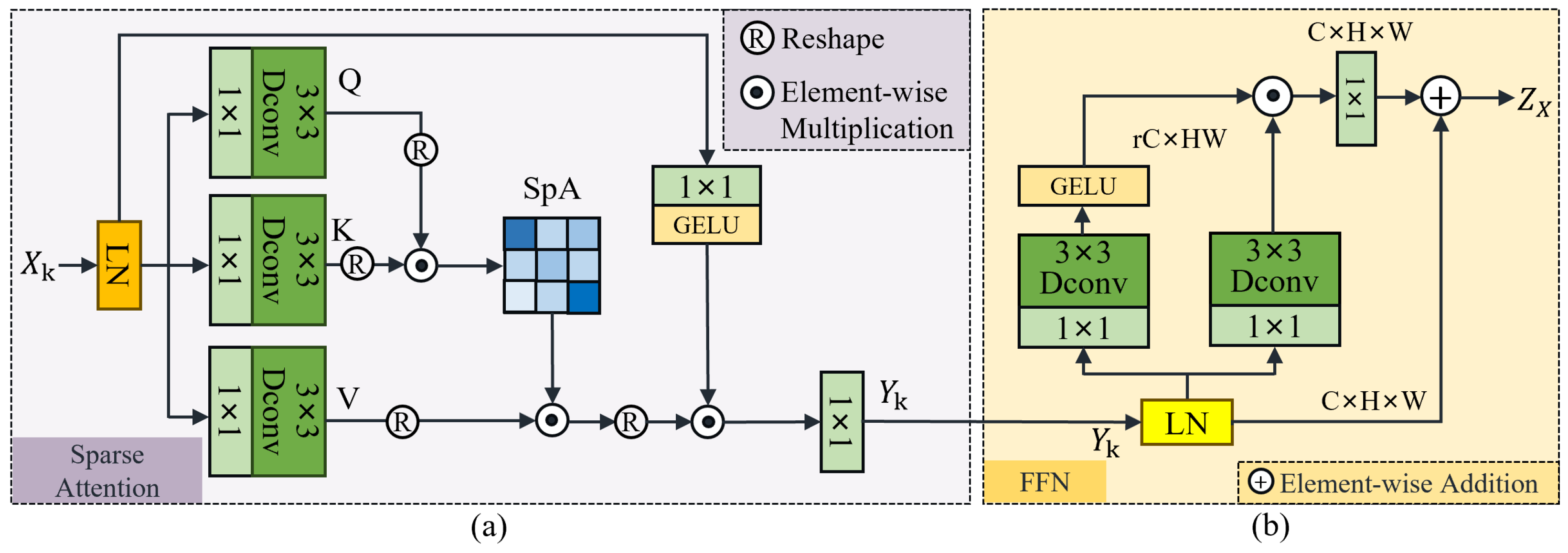
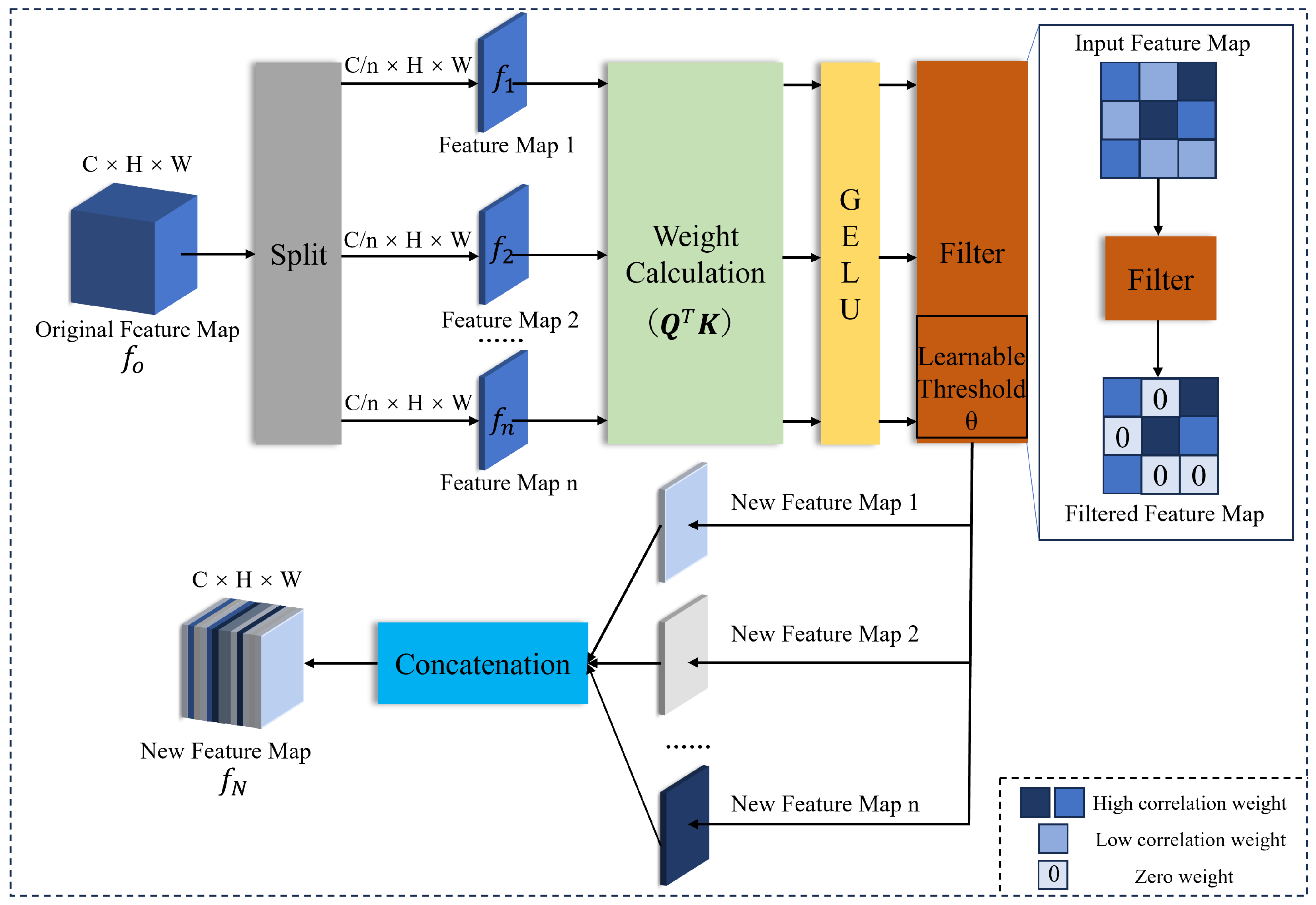

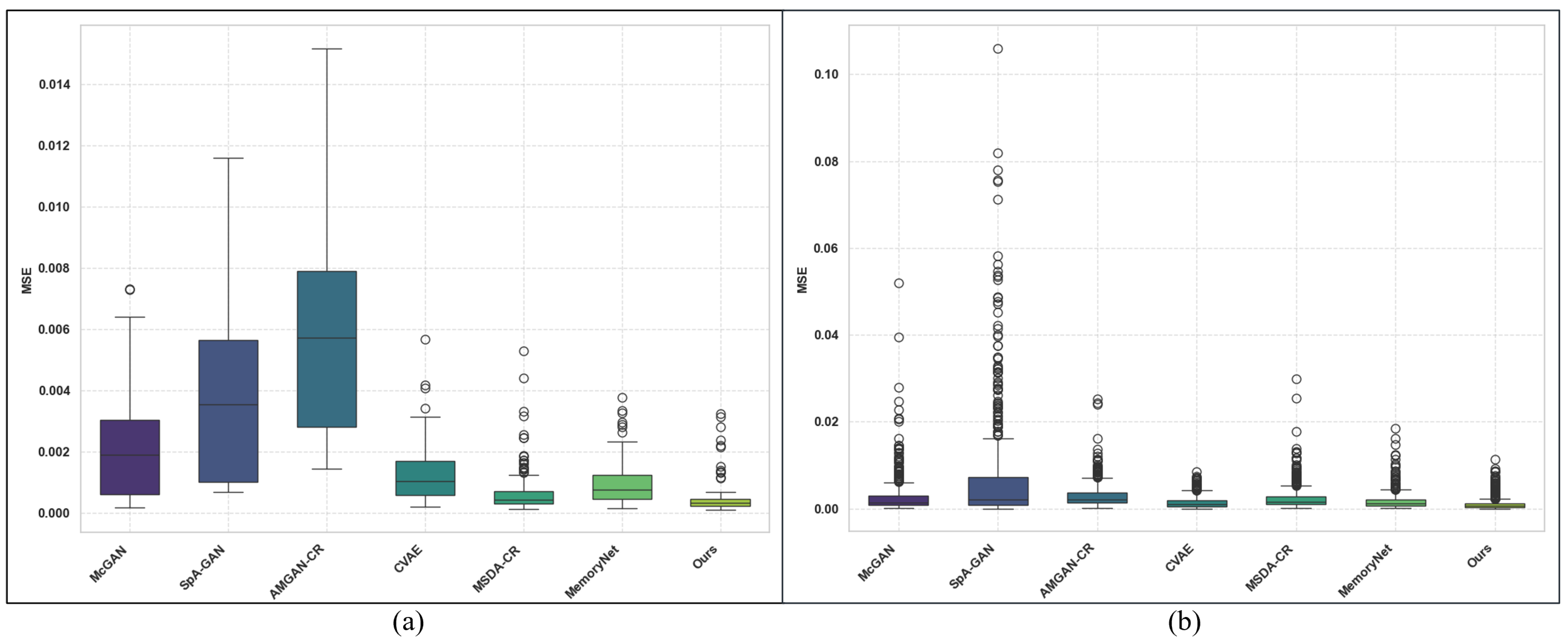
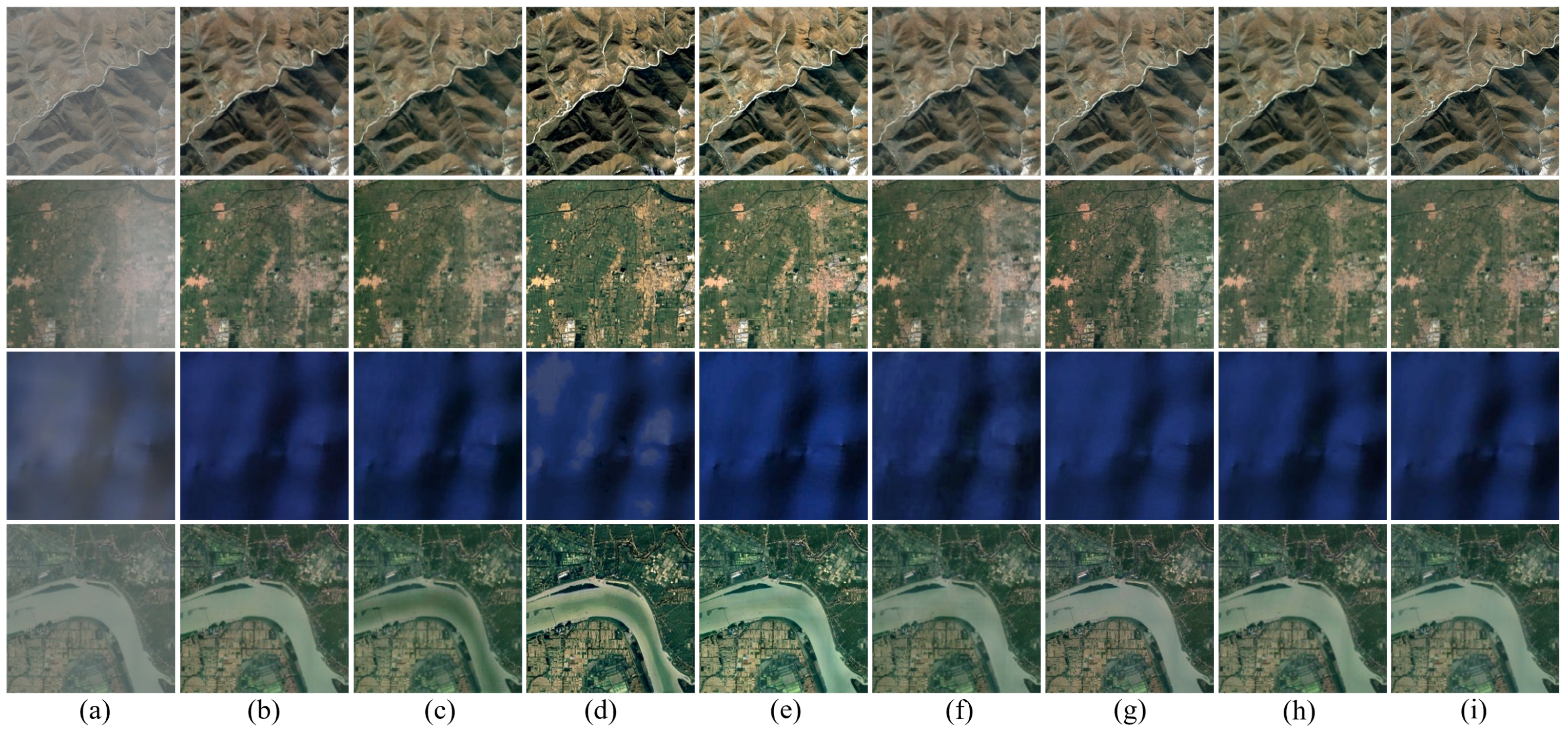
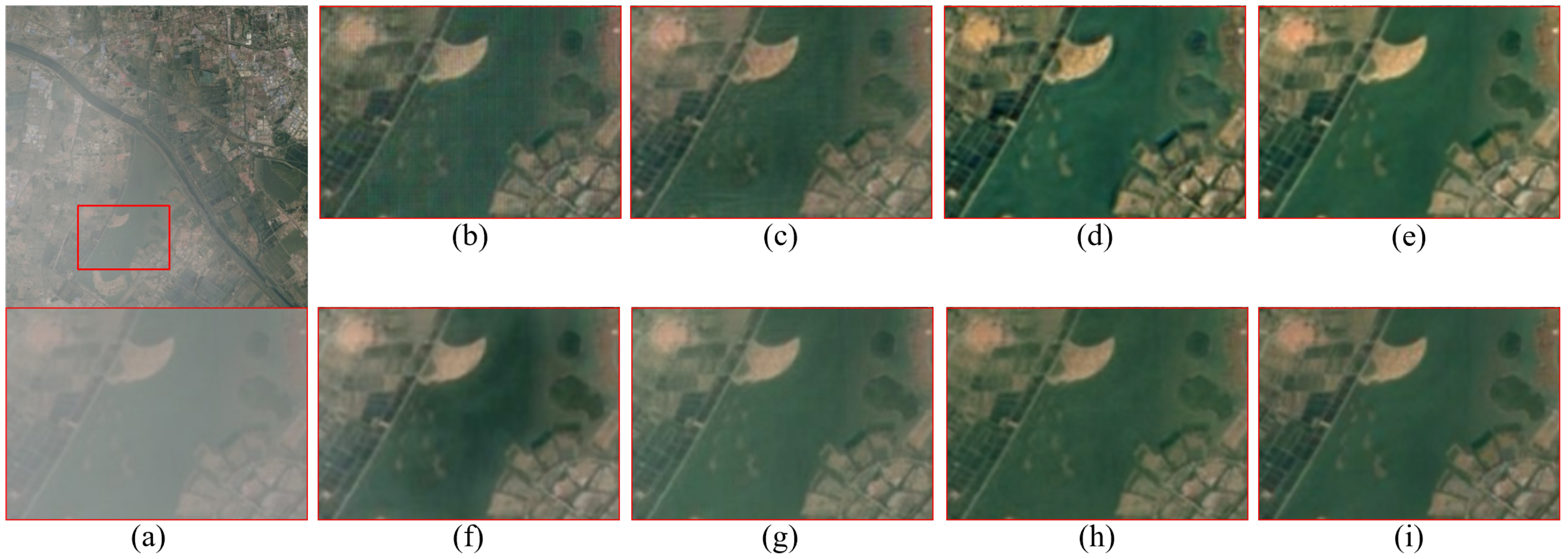
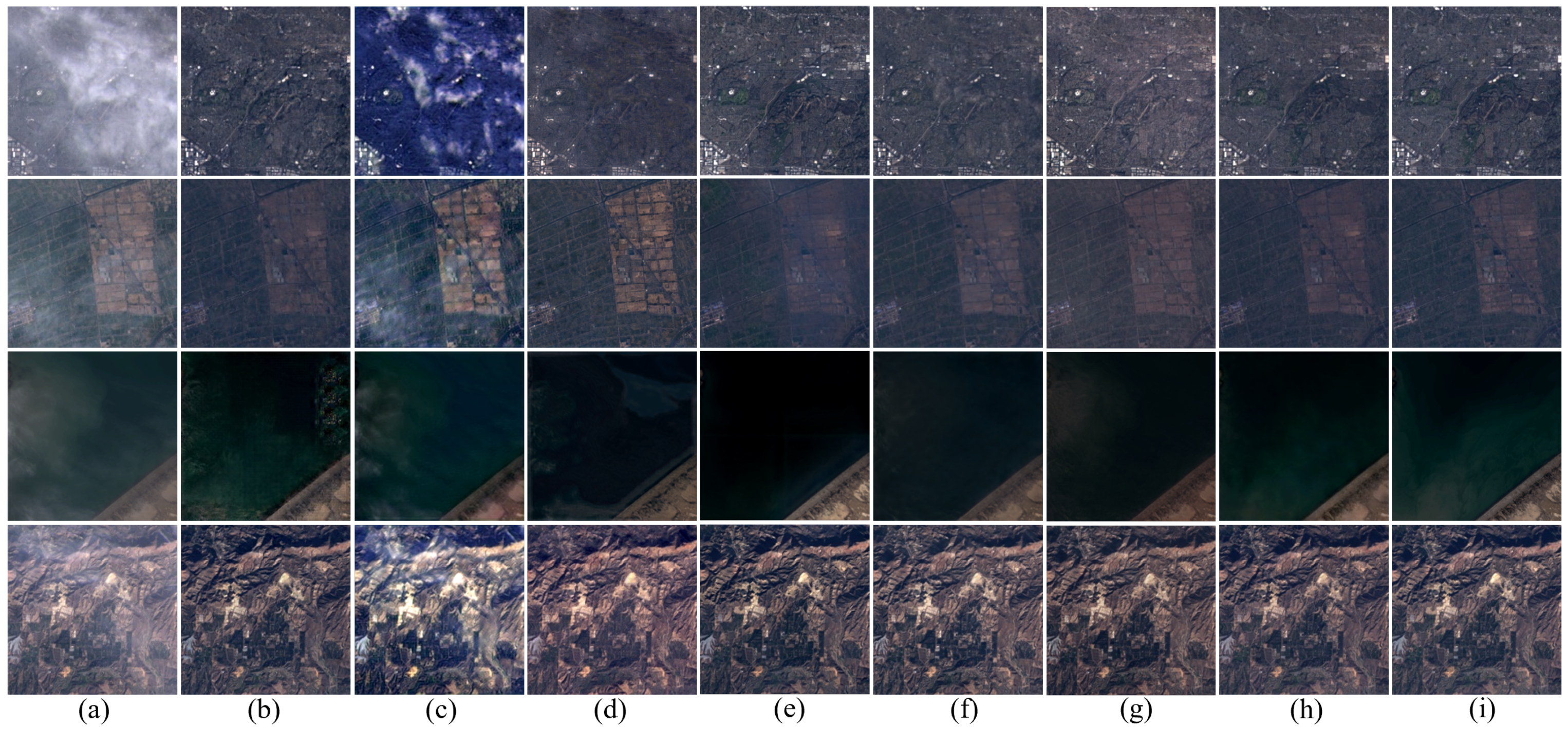
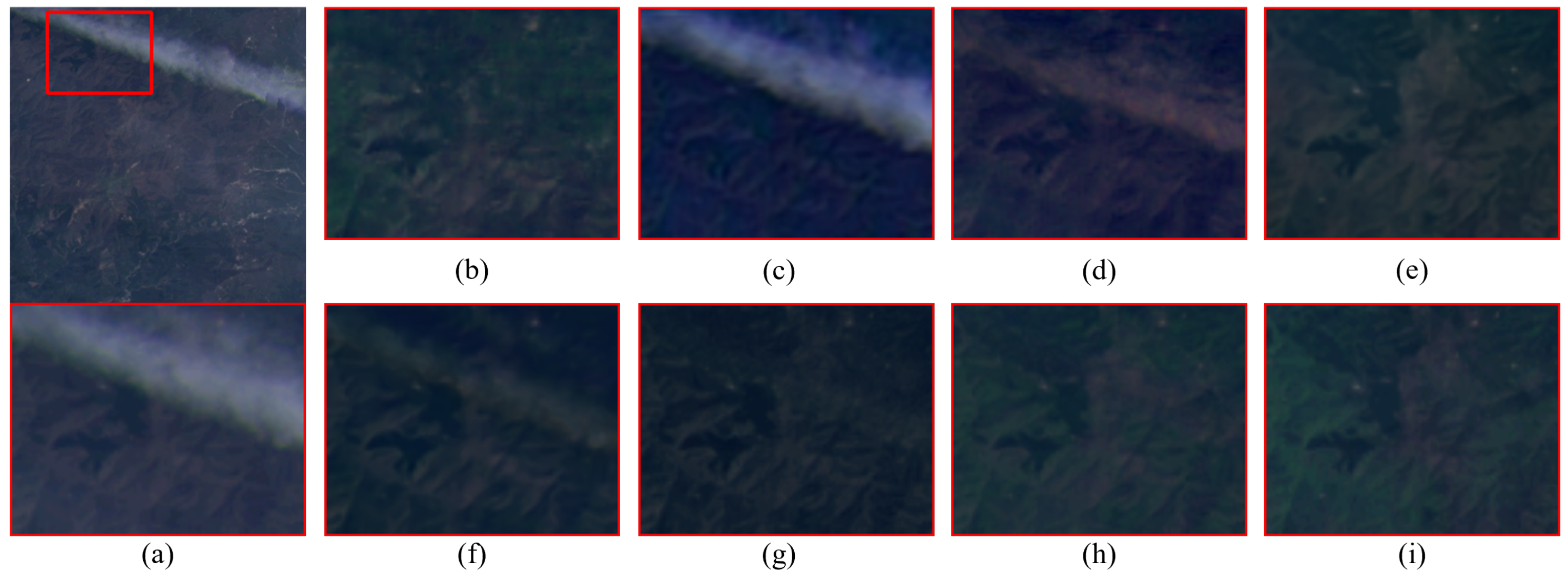
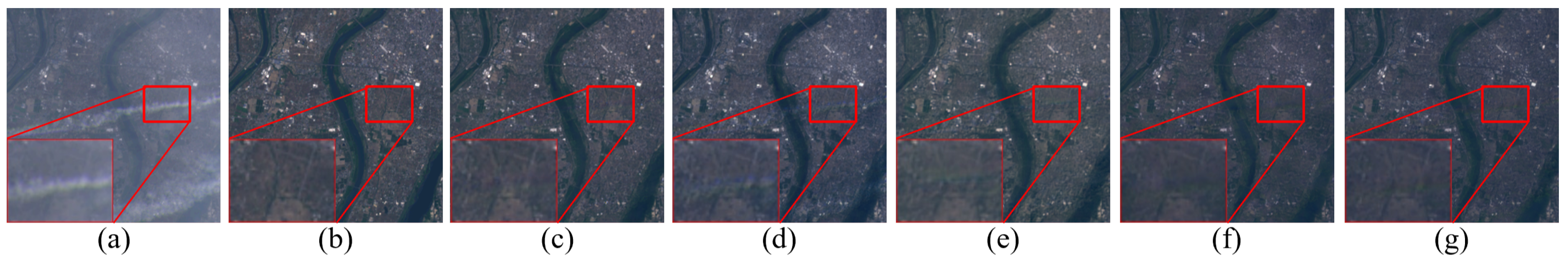

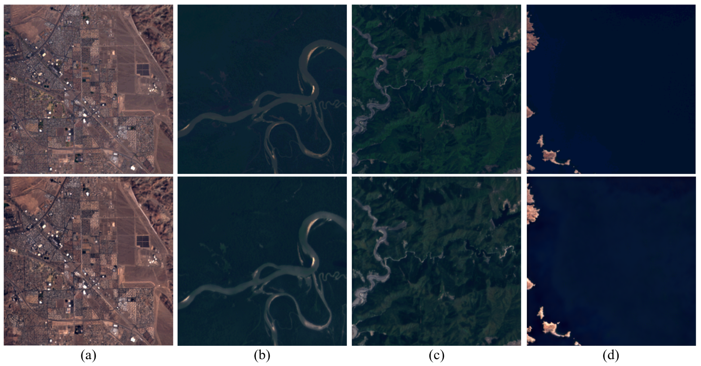
Disclaimer/Publisher’s Note: The statements, opinions and data contained in all publications are solely those of the individual author(s) and contributor(s) and not of MDPI and/or the editor(s). MDPI and/or the editor(s) disclaim responsibility for any injury to people or property resulting from any ideas, methods, instructions or products referred to in the content. |
© 2024 by the authors. Licensee MDPI, Basel, Switzerland. This article is an open access article distributed under the terms and conditions of the Creative Commons Attribution (CC BY) license (https://creativecommons.org/licenses/by/4.0/).