Abstract
Single-tree segmentation on multispectral UAV images shows significant potential for effective forest management such as automating forest inventories or detecting damage and diseases when using an additional classifier. We propose an automated workflow for segmentation on high-resolution data and provide our trained models in a Toolbox for ArcGIS Pro on our GitHub repository for other researchers. The database used for this study consists of multispectral UAV data (RGB, NIR and red edge bands) of a forest area in Germany consisting of a mix of tree species consisting of five deciduous trees and three conifer tree species in the matured closed canopy stage at approximately 90 years. Information of NIR and Red Edge bands are evaluated for tree segmentation using different vegetation indices (VIs) in comparison to only using RGB information. We trained Faster R-CNN, Mask R-CNN, TensorMask and SAM in several experiments and evaluated model performance on different data combinations. All models with the exception of SAM show good performance on our test data with the Faster R-CNN model trained on the red and green bands and the Normalized Difference Red Edge Index (NDRE) achieving best results with an F1-Score of 83.5% and an Intersection over Union of 65.3% on highly detailed labels. All models are provided in our TreeSeg toolbox and allow the user to apply the pre-trained models on new data.
Keywords:
tree crown segmentation; forestry; toolbox; GIS; UAV; vegetation indices; image enhancement 1. Introduction
Conservation and monitoring of forest ecosystems is highly important for economic, ecological and recreational reasons. Being a major place of carbon sequestration, forests play a crucial role globally in mitigating climate change [1]. They are an important setting for biodiversity [2] and serve different functions for humans, such as recreation, hunting, timber production, material and energy utilization, tourism, education, and science, as well as soil, water, and air protection. Worldwide, forest ecosystems are endangered. For example, according to the Federal Forest Inventory of Germany in 2011/2012, approximately one-third of the country was covered by forests [3]. Since 2018, there has been a significant decrease in the forest areas in Germany due to climate change and insect infestations such as the bark beetle. From January 2018 to April 2021, a loss of 5% of all forest areas was detected using satellite data [4]. The federal forest condition report 2023 stated, that due to the drought period between 2018 and 2022, four out of five trees in Germany show visible needle or leaf loss [5]. Thus, monitoring, conservation and sustainable management of forests are critical issues that need to be addressed [4]. In order to obtain an overview of the condition of these forests, forest inventories are implemented throughout the entire German territory as well as in other countries. These inventories gather different types of information such as tree species, age, and diameter at breast height. The fourth forest inventory in Germany was launched in 2021, and will take more than three years from data collection to publication of the results [6].
Consequently, the development of automated airborne acquisition of data is the logical step to take as satellite data do not provide the level of detail required, yet. The lack of data between 2012 and 2021 on the one hand, and the limitations of their spatial reliability on the other hand underlines the need for up-to-date, highly accurate data. The ForestCare project, funded by the German Federal Ministry of Education and Research under the program Digital Green Tech, is one example of research aiming at detecting and classifying individual tree features such as tree species, defoliation, stem form, or diseases, using machine learning techniques on drone or satellite imagery. Its goals were the evaluation of forest growth and the optimization of reforestation measures, as a response to stress factors such as the bark beetle. The project addressed three main aspects: first, the aerial imaging of trees using drones and mobile data collection of the features on the ground; second, the use of these training data to develop a model for tree segmentation, which is the focus of this paper; and finally, based on this, the development of a model that can classify the features [7].
The necessity for fast and precise tree crown segmentation for forest monitoring is related to the constant change in the crown geometries in a forest stand. Thinning, calamities and even annual growth change the canopy structure of forest stands acquired in the preceding year and, therefore, segmentation shapes cannot be used in subsequent years. For reliable forest monitoring on a single tree basis, an annual segmentation of large forest stands is necessary and large efforts by many research groups have been undertaken to tackle the problem of automated segmentation in recent decades: In the 20th century, aerial imagery was manually used for tasks such as detecting diseased trees or assessing tree heights [8,9,10]. Initial attempts to automate tree detection were made in the 1990s [11,12]. During the 2000s, approaches from the Airborne Light Detecting and Ranging (LiDAR) domain dominated tree segmentation [13,14,15]. Currently, in the field of LiDAR segmentation, Deep Learning methods are state of the art [16,17,18]. The emergence of deep neural networks has allowed for segmentation of individual trees in aerial images. Those models are used on data from Unmanned Aerial Vehicles (UAVs) [19,20,21], as well as high-resolution multispectral satellite imagery covering larger geographic areas [22,23,24].
Tree segmentation can generally be grouped into two categories: (1) studies using three dimensional point cloud data in combination with orthophotos and (2) studies using only two dimensional imagery data. Furthermore, segmentation studies investigate different complexities of forests, increasing from agglomerations of solitary trees of one or few species (e.g., parks, plantations) to dense multispecies deciduous forests with heterogeneous tree heights and a closed canopy (e.g., tropical deciduous forests). Coniferous stands can be segmented with higher accuracy than deciduous forests or mixed forests, due to the similar crown geometry of the trees, which also shows more contrasted margins between single crowns in comparison to deciduous trees. The GSD of the analyzed data is also an important factor determining the accuracy of the segmentation. GSDs below 1 cm are time consuming regarding data acquisition (drone flight time) and the orthophoto generation, while they improve segmentation accuracy. In contrast, satellite data (e.g., Sentinel-2 with 10 m GSD in RGB-NIR) do not allow for single tree segmentation due to the comparably poor image resolution. A convenient GSD range used in segmentation studies is 2–10 cm, though commercial satellite data with, e.g., 30 cm GSD are used, as well. Due to the differences in forest complexity and GSD, the segmentation quality varies highly in and between these studies. An Intersection over Union of, e.g., 0.6 can be considered as a sufficient segmentation result, while a tree health assessment based on this segmentation will be affected by an error of 40%. When this 40% includes, e.g., soil pixels or dry grasses on the forest floor this will lead to a false positive identification when searching for trees with low vitality. The effect of a neighbouring tree will depend on the vitality difference between both trees. Due to these implications the Intersection over Union of the segmentation has to be optimized to obtain reliable results on tree properties.
The following paragraph gives an overview on nine recent studies that investigated AI-based single tree segmentation in order of increasing complexity. In cases of the presence of several forest types in one study, only the one with the highest complexity is listed.
Three-dimensional segmentation can be considered as an easier method for segmentation compared to two-dimensional segmentation, as the height information allows one to process tree tops as local maxima and tree margins as local minima. However, it requires collecting and processing a larger amount of data. A study based on LiDAR data segmentation was performed by Zaforemska et al. in 2019 with a GSD of approximately 14 cm [25]. The authors applied five different segmentation algorithms and achieved an F1-Score of 0.87 for non-optimized generalized parameters with a continuously adaptive mean shift algorithm on data from a mixed species forest (sycamore and oak). The data acquisition was performed after the vegetation period, which decreased the complexity of the tree crown structures due to leaf loss and the respective visibility of the organized branch geometries. Wang et al. investigated an urban forest of low complexity and achieved an F1-Score of 0.9 with a watershed-based algorithm at a GSD of 1.7 cm [26]. Liu et al. used three dimensional data to segment more than five different tree species in a forest stand of comparably low complexity [27]. They achieved an F1-Score of 0.9 with a PointNet++ algorithm and on average 8.5 cm GSD for LiDAR and spectral data. Qin et al. segmented trees in a subtropical broadleaf forest with a watershed-spectral-texture-controlled normalized cut (WST-Ncut) algorithm [28]. They achieved a maximum F1-Score of 0.93 for data with a GSD between 10 and 30 cm. Two-dimensional segmentation is more complex, as the information of local minima and maxima cannot be processed. Some studies use effects like sharpening or brightness adjustment in order to highlight light-illuminated tree tops and shadowed crown margins, thereby creating a surrogate for three-dimensional information. Yu et al. [29] achieved an F1-Score of 94% for RGB data analysis of a plantation with low complexity and a downsampled GSD of 2 cm, but they did not state the IoU except that it was larger than 50%, which is insufficient for a reliable analysis of tree features. Lv et al. used RGB spectral data with a GSD of 10 cm of an urban forest with medium complexity [30]. The application of an MCAN algorithm, which is a modification of the Mask R-CNN algorithm, yielded an F1-Score of 88%, while the authors do not state concise IoU values. Safonova et al. developed a three-step tree crown delineation, which they applied on multispectral forest images with a GSD of 3.7 cm [31]. The investigated Bulgarian forest sites were not dense and of intermediate complexity. The intersection of union was very high for mixed forest with approximately 95%, while the F1-Score was not calculated. Dersch et al. investigated the segmentation with CIR sensors, among others, in three forest types (coniferous, deciduous, mixed) with a GSD of 5.5 cm [32]. The best results for the mixed stands were achieved with the single CIR sensor and Mask-CNN (83% F1-Score, 77% IoU). Ball et al. investigated the segmentation in a tropical forest of very high complexity. They used RGB data with a GSD of 8–10 cm and applied the detectree2 algorithm, which is based on Mask-CNN. The F1-Score was 0.6 for trees in the understory and 0.74 for dominating trees, while an IoU was accepted when it was larger than 0.62 [33].
The present study focuses on individual two-dimensional tree segmentation from UAV multispectral imagery and on providing an automated workflow for others to use and/or improve on new data. The main goal is to compare the performance of different algorithms on RGB imagery as well as on different vegetation indices (VIs). Additionally, we evaluate the impact of image enhancement on the segmentation performance and discuss the impact of label quality of accuracy metrics.
2. Materials and Methods
The overall workflow and data used in this study are shown in Figure 1. Data and processing will be described in detail in the following subsections.
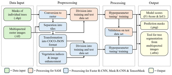
Figure 1.
Flowchart showing the overall workflow of our study.
2.1. Study Area and Data
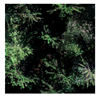
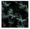
The study area is located in the Black Forest region to the east of Freiburg im Breisgau (for details, refer to Figure 2). The forests are dominated by Picea abies (European spruce), with sporadic existence of Abies alba (European silver fir), Larix decidua (European larch), Acer pseudoplatanus (Sycamore maple), Acer platanoides (Norway maple), Fagus sylvatica (European beech), Fraxinus excelsior (European ash), and Sorbus aucuparia (Mountain ash). The trees show different health conditions, which can affect their crown shape, e.g., due to needle loss. The multispectral UAV data were collected using a DJI Matrice 300 RTK drone system (DJI, Shenzhen, China), with the RedEdge-MX™ Dual Camera sensor (AGEagle, Neodesha, KS, USA). The resulting raster data, with a resolution of approximately 1.3 to 2.3 cm per pixel, consisted of five bands: blue (475 nm), green (560 nm), red (668 nm), near-infrared (840 nm), and RedEdge (717 nm). The segmentation labels were created manually at a very high level of detail based on the multispectral images in a GIS (ArcGIS Pro 2.8, Environmental Systems Research Institute (ESRI), Redlands, CA, USA). In total, there are 1096 labeled trees in the study area (compare Table 1 for details about tree species).
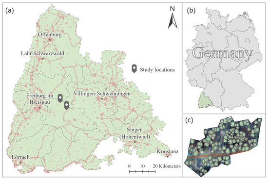
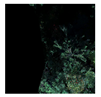
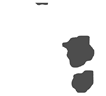
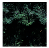
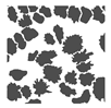
Figure 2.
Study areas in Germany: (a) The sampling locations near Freiburg im Breisgau; (b) Location of the study area is in Germany; (c) Example of some trees with segmentation masks.

Table 1.
Labeled trees by species in the study area.
2.2. Preprocessing for Deep Learning
Preprocessing of data included creating tiles and masks for Deep Learning as well as the calculation of vegetation indices: (1) We converted the shapefiles into binary masks with the extent of their corresponding multispectral images. For Faster-RCNN, Mask R-CNN and TensorMask, the raster images were divided into 1200 by 1200 pixel tiles with a 4% overlap between tiles. Additionally, the dataset was transformed into the COCO-JSON format [34].
(2) Subsequently, all data were randomly split into training and test datasets (approximately 10:1); validation was automatically set apart by the Deep Learning networks. The training dataset contains approximately 800 trees over an area of approximately 4.3 hectares, the test dataset contains approximately 80 trees over a total area of approximately 0.4 hectares.
(3) In addition, data were processed using three image-enhancement methods to improve their quality using OpenCV, an open-source library for image processing: A: Denoising, which plays an important role in digital image processing, because it can remove unwanted noise and improve image quality [35,36]. B: Histogram stretching, which enhances the image contrast by adjusting pixel values to cover the full brightness range. It makes image details more visible [37]. C: Deblurring, which optimizes the image sharpness [38]. We use this second, improved, dataset to evaluate the impact of image enhancement on model performance.
(4) Additionally, different VIs were calculated to assess their importance for the segmentation task. VIs use combinations of spectral bands to show the health, density and other important aspects of vegetation [39,40]. A total of eleven indices were evaluated and are listed in Table 2.
Table 2.
Overview of vegetation indices tested in the paper.
2.3. Experiments and Deep Learning Models
For our experiments, we used Faster R-CNN, Mask R-CNN, TensorMask and SAM as instance-segmentation models. A brief description of each model’s characteristics will be given in the following, Table 3 shows a list of all conducted experiments and Table A1 and Table A2 in the Appendix A show the optimum hyperparameter settings for the respective models found during fine-tuning.
Table 3.
List of conducted experiments.
For Faster R-CNN, Mask R-CNN, TensorMask, and SAM, certain hyperparameters, such as the Bias Learning Rate Factor, have a significant impact on performance metrics like IoU and F1-Score and best values were chosen for the final model. Other important hyperparameters include the Learning Rate, Warm-up Factor, Number of Decays, and Weight Decay. Too many Maximal Iterations lead to overfitting, while a smaller Batch Size and a higher Learning Rate yielded better results for our specific dataset.
As TensorMask is not an R-CNN, somewhat different hyperparameters were tested. The best results were achieved by tuning parameters like the Number of Decays, Learning Rate Gamma and Mask Loss Weight, crucial for finding the global minimum and influencing the quality of mask predictions. The Number of Convolutions showed that increased complexity leads to overfitting, while good regularization at higher values improved performance. Other important hyperparameters include Maximum Iterations, Batch Size, Learning Rate, Warm-up Factor, and Momentum.
Faster R-CNN, short for Faster Region-Based Convolutional Neural Network (R-CNN), was the first model developed for object detection. A Feature Pyramid Network (FPN) is utilized to extract features at various scales. The core element of the architecture is the Region Proposal Network (RPN), which suggests regions likely to contain objects based on the extracted features. These regions are standardized in size using the RoI (Regions of Interest) pooling layer and then processed within an R-CNN. The results are further refined by a classification and object detection head. For details, refer to [52,53]. We use ResNet-101 as a backbone during our experiments.
The structure of Mask R-CNN closely resembles that of Faster R-CNN, with ResNet-50 serving as the backbone network in combination with FPN. From the extracted features, RoIs are proposed via RPN. To standardize the sizes of these regions, it employs an RoI align layer. Next, these regions are refined in an R-CNN module. A key difference from the original Faster R-CNN is that Mask R-CNN additionally fine-tunes its results with an instance-segmentation head [52,54].
TensorMask employs the dense sliding window method for feature extraction. In this approach, a window slides over an input image, and at each step, a Convolutional Backbone is executed to extract features and generate mask proposals. These mask proposals are represented as 4D tensors, where the dimensions correspond to the height, width, number of channels for classes, and pixel values of the mask. Similar to Mask R-CNN, TensorMask utilizes ResNet-50 as the backbone in combination with FPN. The mask proposals are then processed in three branches: one for classification, one for object detection through bounding boxes, and a third for predicting segmentation masks [52,55].
SAM (Segment Anything Model) was pre-trained on 1.1 million images and 1.1 billion masks, using techniques from both computer vision and natural language processing (NLP). SAM utilizes an image encoder to generate an image embedding for each input image, representing its visual features in a numerical vector format. Subsequently, a prompt encoder is employed to encode various types of prompts, such as points, masks, bounding boxes, or text, into embedding vectors. Following this, a mask decoder is utilized, using the embedding vectors from the image encoder and prompt encoder to accurately generate segmentation masks [56,57]. In our first set of experiments we conduct extensive hyperparameter tuning using grid search (see Table A1 and Table A2 for best settings) for all architectures and compare model performance on RGB data (compare Table 3).
Model performance was assessed using the F1-Score and IoU on our test dataset. The F1-Score is the harmonic mean between Precision and Recall (see Equation (1)). Precision calculates the ratio of True Positives (TPs) and the total number of positive predictions, which includes True Positives and False Positives (FPs) (see Equation (2)). Recall, on the other hand, shows the ratio of True Positives and the total number of actual positive instances, containing True Positives and False Negatives (FNs) (Equtaion (3)) [58]:
The Intersection over Union (IoU) is defined as the ratio between the area of overlap and the area of union between ground truth (A) and the bounding boxes or segmentation masks predicted by model (B) (Equation (4)) [59]:
2.4. TreeSeg Toolbox
Based on the optimal results obtained, a tool was developed to automatically calculate instance segmentation of individual trees in multispectral images. The output of the tool is a shapefile containing individual tree crowns. The toolbox implementation was conducted using Python (3.9.11 for Faster R-CNN, Mask R-CNN and Tensormask, 3.8.18 for SAM) and can be added to ArcGIS Pro (v3.1).
3. Results
The prediction mask results are shown in Table 4 (model comparison) and Table 5 (data engineering) and the result scores of all experiments are listed in Table 6 (model comparison) and Table 7 (data engineering).
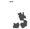
Table 4.
Model comparison results. Predictions from Faster R-CNN, Mask R-CNN, TensorMask and SAM, as well as ground truth masks and original images, are shown.
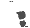
Table 5.
Example prediction masks using Normalized Difference Red Edge Index (NDRE), Green Leaf Index (GLI), Relative Vegetation Index (RVI) and Image Enhancement, as well as ground truth masks and original images, are shown.
Table 6.
Evaluation results of the models using RGB-images.
Table 7.
Image enhancement and vegetation index evaluation results on Faster R-CNN.
3.1. Model Comparison
Faster R-CNN achieved the highest F1-Score at 76.8%, followed by Mask R-CNN with 69.3%. Faster R-CNN also yielded the highest IoU at 58.2%, with Mask R-CNN closely behind scoring at 58.1%. In contrast, SAM achieved the poorest results with an IoU of 21% and an F1-Score of 33%. Precision and Recall showed balanced results for Faster R-CNN, Mask R-CNN and TensorMask. For SAM, Precision had a low value of 25% and Recall had a rather high value of 81.5%.
Qualitative results in Table 4 look smoother for all models than the original labels. Only SAM showed low quality results, as expected from the quantitative assessment.
3.2. Impact of Data-Engineering Methods
Results of testing image enhancement and combinations of spectral bands and vegetation indices are presented in Table 7. Data-engineering methods were only tested on Faster R-CNN, as this architecture performed best in the model comparison. Despite an average F1-Score of 74 %, image enhancement achieved the second-highest IoU at 63.3%. Including vegetation indices, however, had a much higher impact on model performance: The highest F1-Score (83.5%) and IoU (65.3%) was achieved by including the NDRE. Other indices with F1-Scores above 80% are the GLI and the RVI. Lowest scores were obtained by including the EVI with an IoU of 48.2 % and an F1-Score of 60.8%. Precision and Recall ranged between 64 and 80% with highest Precision resulting from image enhancement and by including the RVI.
3.3. SegTree Toolbox
The trained models, toolbox and user instructions are provided on GitHub (https://github.com/soenke-sp/TreeSeg). The input data required to run the tool consist of a UAV multispectral image with channels for RGB, near-infrared and red edge. Subsequently, one of the four tested models can be selected for inference. For Faster R-CNN, Mask R-CNN and TensorMask, the NDRE of the multispectral image is calculated. Then, instance segmentation is performed and a shapefile containing the individual trees is calculated. It should be noted that, due to the optimum hyperparameter configuration, the calculation using SAM may take more than a day depending on the hardware resources. However, as this model shows poor results, it is not recommended but still included for transparancy of results.
4. Discussion
We will first discuss our results with respect to other approaches described in the introduction and then proceed to discussing our results and problems involved in data collection and labelling details.
4.1. Comparison to Other Approaches
There are several promising approaches in the field of individual tree segmentation on high-resolution data, encompassing passive sensing as well as active sensing methods or combinations. Very good results have been achieved using LiDAR data or a combination with spectral data, though these approaches are not feasible for large-scale monitoring, yet. For example, Wang et al. achieved accuracies higher than 90% [26] and an F1-Score of 93.1% on urban temperate forest areas using a watershed algorithm. However, the segmentation masks exhibit a lower level of detail compared to the masks utilized in this paper and accuracy metrics are therefore not directly comparable to our results. On subtropical urban forests, Qin et al. combined LiDAR, hyperspectral and ultrahigh-resolution RGB data, using the watershed algorithm to obtain an F1-Score of 91.8% [28]. Even though accuracy is higher, acquiring such multi-modal high-resolution data is not feasible on a large scale in forestry. In the field of Deep Learning, Liu et al. used deep neural networks and PointNet++ and reached an F1-Score of 91%. Additionally, by using the Li2012 algorithm, they achieved an F1-Score of around 90%, also on subtropical forests [27]. Using the mean shift clustering algorithm, Zaforemska et al. reached an F1-Scores over 90% on temperate forests [25]. Yu et al. achieved an F1-Score of 94.6% using Mask R-CNN on mountainous forest plantations. In addition to the image data, point cloud elevation data were also utilized [29]. This clearly indicates that LiDAR based segmentation is superior to two-dimensional segmentation, while such methods are at present restricted to small areas in the sub-100 ha range. The long UAV flight times to acquire detailed data and the high processing costs for creating the point clouds for orthophoto creation prevent such methods from reaching the goal of a nation-wide large-scale forest monitoring.
In the field of image segmentation with spectral data, Safonova et al. used the ITCD algorithm on data from a temperate forest to score an IoU of around 93% . These excellent results were achieved on labels with a lower level of detail than our labels as well as a lower tree density, making identification of single-trees less challenging [31]. Vegetation indices as metrics for capturing tree health [40], have a high potential for segmentation tasks and several studies agree with our findings when using VIs: The above-mentioned study by Wang et al., for example, achieved an F1-Score of 93.1%, using the Normalized Difference Greenness Index (NDGI) [26,60], which agrees with our findings highlighting the importance of VIs. Along the same lines, Qin et al. used different vegetation indices, such as the Enhanced Vegetation Index (EVI), and achieved an F1-Score of 91.8% [28,61]. Ulku et al., on the other hand, experimented with different Deep Learning models and different VIs and achieved the highest IoU of 92.1% when Near Infrared input was used for DLinkNet [50,62]. The Normalized Difference Vegetation Index (NDVI) on the same model only reached an IoU of 86.1%. The single tree masks also exhibited a reduced level of detail compared to this paper.
With our complex forest setting and labels of a very high level of detail, Faster R-CNN achieved the best results with an F1-Score of 84% on a combination of the NDRE, R, G and of 81% using the GLI in combination with R and G bands (Table 7). With respect to the model’s performance, Faster R-CNN achieved the best results in our setting compared to Mask R-CNN, TensorMask or SAM (compare Table 6). This does not agree with the findings of Lv et al. who achieved a higher F1-Score for Mask R-CNN (82.6%) in comparison to Faster R-CNN (79.5%) in urban forests. This might be due to differences in the datasets. Lv et al. used a larger dataset containing 32,840 trees [30], contrasting with approximately 800 trees in the training dataset used in this study (refer to Table 1). The larger dataset may be more suitable for the high complexity of Mask R-CNN in comparison to Faster R-CNN.
While there are no further comparative studies for the better-performing model Faster R-CNN, there are significantly more studies available for Mask R-CNN about single tree instance segmentation in forests. Apart from Ball et al., who achieved an F1-Score of 63.4% for understory trees and 0.74% for dominating trees at comparably low GSD in a complex tropical forest canopy [33], some other studies have achieved better scores than those reported in this paper [29,32]. It is worth noting that Ball et al. used segmentation on data from tropical forests [33], which is comparable to our study site and explains the lower performance of the segmentation in both studies. All studies with higher performance used more training data compared to the dataset used in this study, which is not surprising given the nature of these architectures and/or less complex settings such as the study of Yu et al. who segmented a plantation forest with higher contrasts and clearer spacings between trees. The Bavarian forest investigated by Dersch et al. consisted of only two species (spruce and beech), while our study site contained three conifer species and five deciduous tree species. These differences explain the better segmentation results in Yu et al. and Dersch et al., as the geometric complexity of the investigated forests was much lower than in the mixed forest stands investigated here. It appears that the higher the complexity of the forest canopy, the higher is the relative amount of pixels that are within the segmentation polygon, but do not belong to the tree. In our study, the IoU was 58%, which is a success when contrasted against the high geometrical and species complexity of the forest and the high level of details of the ground truth data. Many studies do not include the IoU percentage, although in terms of tree analysis this is one of the most important segmentation quality parameters. Silva et al. [63] reported an IoU of 50% for a pine tree forest, Zheng et al. and Ball et al. accepted true positive segmentation at a IoU above 50% [33,64], while Dersch et al. [32] presented an IoU of 77% for a two- species deciduous forest of medium density. While in 2016 Silva et al. achieved a low IoU for a forest with low complexity, the team around Dersch et al. performed better for a forest of higher complexity in 2023, which shows the improvement of the IoU over time. Yu et al. and Ball et al. proposed that an IoU of 50% was considered as sufficient for true positive segmentation, which seems to be widely accepted in the literature on tree segmentation [29,33]. Many other studies do not state the IoU at all [25,26,27,28,30]. Our study achieved an IoU of maximum 65% for a forest with a very high complexity and detailed ground truth data. This shows that instant segmentation of single trees in managed forests is a very challenging problem, which is not resolved, yet. Even with an IoU of, e.g., 80%, 20% of the assigned pixels of a tree crown would still contain false information, thereby distorting further data analysis, e.g., crown vitality assessment. It is well known that, e.g., soil-reflectance characteristics are comparable to damaged tree crowns that show yellow or brown discoloration. Adding a significant share of soil pixels to a healthy tree crown would render the crown damage-assessment result to a false positive information. Further studies on single tree crown segmentation should address this aspect by improving the IoU rather than the F1-Score in order to facilitate the practical applicability of the results for tree analysis. The widely accepted threshold of 50% for the IoU is insufficient for further purpose-driven analysis of tree crown characteristics as results might be severely affected by these wrongly assigned pixels contain false information. For TensorMask and SAM, there are no further studies on the topic, according to the knowledge of the authors. Apparently, TensorMask performs similarly to Mask R-CNN in general [55,65,66]. But with an F1-Score of 52.7% in this study, it did not perform sufficiently well (see Table 6). SAM shows such poor results that it will not be discussed further.
4.2. Discussion of Our Experiments
Comparing the different models evaluated during this study, we found the R-CNN models performed much better than TensorMask and SAM. During hyperparameter tuning, we found that finding the optimum parameters for each model is of crucial importance for the learning result (compare Table A1 and Table A2). With respect to SAM, the bad performance might be due to the very different data it was trained on. The performance difference between Faster R-CNN and Mask R-CNN is marginal when comparing the IoU, Precision and Recall due to the similarity of the architectures. A much greater impact is due to data enhancement and, above all, by including VIs in the training process (compare Table 6 and Table 7). We see an improvement of 5% due to image enhancement in the IoU and of 6% due to including the NDRE. This indicates that image enhancement enables Faster R-CNN to achieve a better overlap between predicted masks and ground truth masks [59]. However, on the other hand, the shape of the masks appears to lack Precision and Recall accuracy [58]. This could be attributed to the use of filters in image enhancement which leads to blurring boundaries between trees and the background [67,68].
Some indices, such as NDRE or RVI, use the near-infrared or red edge wavelength range in their computation. RVI achieved an F1-Score of 80.5% . However, the second-best result was achieved by the GLI with 80.6%, which only employs the standard RGB bands (see Table 6 and Table 7). Our best result agrees with other authors who achieved good segmentation results using VIs that include infrared bands [26,28,60,61], though the GLI also performs well. One major aspect of our results is the level of detail of the label data. As shown in Table 4 and Table 5, the initial labels were digitized around single branches with very refined edges, while the output labels are much coarser or generalized. As mentioned in the previous section, this partly explains our lower IoUs in comparison to those reported by other authors who compare to coarser labels. However, it also shows that the models have not learned this level of detail, which might be due to the small amount of training data and should be further investigated. This, however, is difficult as such high-quality labels are scarce. Additionally, it is important to note that comparability to other results is limited since these studies focus on different types of forests with different tree species composition and dataset sizes. In particular, less dense and less complex forests will result in much better segmentation results given the same algorithm.
5. Conclusions
In this study, we evaluated different instance-segmentation models with respect to performance as well as the impact of image enhancement. With an F1-Score of 84%, Faster R-CNN outperformed the other models on NDRE data in combination with the red and green band.
The goal of an automated, widely applicable workflow for forestry is our vision in providing these models as a toolbox for other researchers to use and further develop. We showed the importance of using VIs compared to spectral bands and found that, with respect of the level of detail in labels, there is still a lot of work to be carried out to meet the requirements of automatically extracting single branches of the tree crowns. This is a requirement for downstream tasks such as health assessment or early detection of infestations and, thus, of utter importance for applied forestry. Most studies, as discussed in Section 4, use coarser labels for tree crown segmentation, achieving better results in terms of accuracy metrics, but not in terms of the required level of detail. The main issue here is that such detailed labels are scarce and much more data would be required for the models to learn well. A model trained on a larger and more diverse dataset would offer the possibility to generalize on different forest types and even ecosystems. Along these lines, our intent of sharing our models on GitHub is to encourage further production of high-quality labels. We hope, that with our toolbox and the models provided for future research, we contribute to further refining models that are suited to be applied on a larger scale to support applied forestry.
Author Contributions
Conceptualization, M.B. and S.P.; methodology, S.S., M.B. and S.P.; formal analysis, S.S.; resources, M.B.; data curation, S.P. and S.S.; writing—original draft preparation, S.S., S.P. and M.B.; writing—review and editing, M.B., S.P. and S.S.; supervision, S.P. and M.B.; project administration, S.P.; funding acquisition, S.P. All authors have read and agreed to the published version of the manuscript.
Funding
Publication supported by the publication fund of the Technical University of Applied Sciences Würzburg-Schweinfurt. The project ForestCare was funded by the German Ministry for Education and Science under the grant number 033D014A.
Data Availability Statement
Data are contained within the article.
Conflicts of Interest
The authors declare no conflicts of interest.
Appendix A
Table A1.
Optimal hyperparameter configurations for Faster R-CNN, Mask R-CNN and TensorMask.
Table A1.
Optimal hyperparameter configurations for Faster R-CNN, Mask R-CNN and TensorMask.
| Hyperparameter | Faster R-CNN | Mask R-CNN | TensorMask |
|---|---|---|---|
| Maximal Iterations | 40,000 | 40,000 | 40,000 |
| Batch Size | 1 | 2 | 8 |
| Learning Rate | 0.001 | 0.001 | 0.0001 |
| Warm-up Factor | 0.001 | 0.001 | 0.001 |
| Warm-up Method | linear | linear | linear |
| Number of Decays | 3 | 3 | 3 |
| Learning Rate Gamma | 0.01 | 0.01 | 0.5 |
| Bias Learning Rate Factor | 2 | 2 | 2 |
| Weight Decay for Bias | 0.001 | 0.001 | 0.001 |
| Momentum (Based Gradient Descent) | 0.85 | 0.85 | 0.95 |
| Nesterov’s Accelerated Gradient | true | true | false |
| Weight Decay | 0.0001 | 0.0001 | 0.0001 |
| Weight Decay for Normalization | 0.05 | 0.05 | 0.01 |
| RoI (Region of Interest) Head Batch Size | 1024 | 1024 | 128 |
| Focal Loss Alpha | 0.2 | ||
| Focal Loss Gamma | 3 | ||
| Score Threshold Test | 0.001 | ||
| Non-Maximum Suppression (NMS) Threshold Test | 0.5 | ||
| Number of Convolutions | 2 | ||
| Mask Channels | 256 | ||
| Mask Loss Weight | 2 | ||
| Mask Positive Weight | 1.5 | ||
| Aligned | false | ||
| Tensorbipyramid | false | ||
| Classification Channels | 64 |
Table A2.
Optimal hyperparameter configuration for SAM.
Table A2.
Optimal hyperparameter configuration for SAM.
| Hyperparameter | Value |
|---|---|
| Points per Side | 32 |
| Prediction Intersection over Union (IoU) Threshold | 0.5 |
| Stability Score Threshold | 0.5 |
| Stability Score Offset | 1 |
| Box Non-Maximal Suppression (NMS) Threshold | 1 |
| Crop n Layers | 5 |
| Crop Overlap Ratio | 0.5 |
| Crop n Points Downscale Factor | 2 |
References
- Raihan, A.; Begum, R.A.; Mohd Said, M.N.; Abdullah, S.M.S. A Review of Emission Reduction Potential and Cost Savings through Forest Carbon Sequestration. Asian J. Water Environ. Pollut. 2019, 16, 1–7. [Google Scholar] [CrossRef]
- Brockerhoff, E.G.; Barbaro, L.; Castagneyrol, B.; Forrester, D.I.; Gardiner, B.; González-Olabarria, J.R.; Lyver, P.O.; Meurisse, N.; Oxbrough, A.; Taki, H.; et al. Forest biodiversity, ecosystem functioning and the provision of ecosystem services. Biodivers. Conserv. 2017, 26, 3005–3035. [Google Scholar] [CrossRef]
- Thünen Institut. Dritte Bundeswaldinventur-Ergebnisdatenbank 2012. Available online: https://www.thuenen.de/de/fachinstitute/waldoekosysteme/projekte/waldmonitoring/projekte-bundeswaldinventur/bundeswaldinventur (accessed on 30 April 2024).
- Thonfeldt, F. Sorge um den Deutschen Wald. Dtsch. Zent. Luft Raumfahrt 2022. Available online: https://www.dlr.de/de/aktuelles/nachrichten/2022/01/20220221_sorge-um-den-deutschen-wald (accessed on 30 April 2024).
- BMEL. Ergebnisse der Waldzustandserhebung 2023; BMEL Report; Bundesministerium für Ernährung und Landwirtschaft: Berlin, Germany, 2023; Available online: https://www.bmel.de/DE/themen/wald/wald-in-deutschland/waldzustandserhebung.html (accessed on 30 April 2024).
- BMEL. Verordnung üBer die Durchführung Einer Vierten Bundeswaldinventur (Vierte Bundeswald-Inventur-Verordnung—4. BWI-VO); BMEL: Berlin, Germany, 2019; p. 890. [Google Scholar]
- BMBF. ForestCare—Einzelbaumbasiertes, Satellitengestütztes Waldökosystemmonitoring; BMBF: Berlin, Germany, 2019. [Google Scholar]
- Heller, R.; Aldrich, R.C.; Bailey, W.F. An evaluation of aerial photography for detecting southern pine beetle damage. In Proceedings of the Society’s 25th Annual Meeting, Hotel Shoreham, Washington, DC, USA, 8–11 March 1959. [Google Scholar]
- Rogers, E.J. Estimating Tree Heights from Shadows on Vertical Aerial Photographs. J. For. 1949, 47, 182–191. [Google Scholar] [CrossRef]
- Andrews, G.S. Tree-Heights From Air Photographs By Simple Parallax Measurements. For. Chron. 1936, 12, 152–197. [Google Scholar] [CrossRef]
- Brandtberg, T.; Walter, F. Automated delineation of individual tree crowns in high spatial resolution aerial images by multiple-scale analysis. Mach. Vis. Appl. 1998, 11, 64–73. [Google Scholar] [CrossRef]
- Gougeon, F.A. A Crown-Following Approach to the Automatic Delineation of Individual Tree Crowns in High Spatial Resolution Aerial Images. Can. J. Remote Sens. 1995, 21, 274–284. [Google Scholar] [CrossRef]
- Reitberger, J.; Schnörr, C.; Krzystek, P.; Stilla, U. 3D segmentation of single trees exploiting full waveform LIDAR data. ISPRS J. Photogramm. Remote Sens. 2009, 64, 561–574. [Google Scholar] [CrossRef]
- Reitberger, J.; Heurich, M.; Krzystek, P.; Stilla, U. Single Tree Detection in Forest Areas with High-Density LIDAR Data. Int. Arch. Photogramm. Remote Sens. Spatial Inf. Sci. 2007, 36, 139–144. [Google Scholar]
- Tiede, D.; Lang, S.; Hoffmann, C. Supervised and Forest Type-Specific Multi-Scale Segmentation for a One-Level-Representation of Single Trees; Elsevier B.V.: Amsterdam, The Netherlands, 2006. [Google Scholar]
- Yang, J.; El Mendili, L.; Khayer, Y.; McArdle, S.; Hashemi Beni, L. Instance Segmentation of LiDAR Data with Vision Transformer Model in Support Inundation Mapping under Forest Canopy Environment. ISPRS Arch. Photogramm. Remote Sens. Spatial Inf. Sci. 2023, 48, 203–208. [Google Scholar] [CrossRef]
- Straker, A.; Puliti, S.; Breidenbach, J.; Kleinn, C.; Pearse, G.; Astrup, R.; Magdon, P. Instance Segmentation of Individual Tree Crowns with YOLOv5: A Comparison of Approaches Using the ForInstance Benchmark LiDAR Dataset. Open Photogramm. Remote Sens. J. 2023, 9, 100045. [Google Scholar] [CrossRef]
- Wang, D. Unsupervised Semantic and Instance Segmentation of Forest Point Clouds. ISPRS J. Photogramm. Remote Sens. 2020, 165, 86–97. [Google Scholar] [CrossRef]
- Li, Y.; Chai, G.; Wang, Y.; Lei, L.; Zhang, X. ACE R-CNN: An Attention Complementary and Edge Detection-Based Instance Segmentation Algorithm for Individual Tree Species Identification Using UAV RGB Images and LiDAR Data. Remote Sens. 2022, 14, 3035. [Google Scholar] [CrossRef]
- Zhang, C.; Zhou, J.; Wang, H.; Tan, T.; Cui, M.; Huang, Z.; Wang, P.; Zhang, L. Multi-Species Individual Tree Segmentation and Identification Based on Improved Mask R-CNN and UAV Imagery in Mixed Forests. Remote Sens. 2022, 14, 874. [Google Scholar] [CrossRef]
- Xi, X.; Xia, K.; Yang, Y.; Du, X.; Feng, H. Evaluation of Dimensionality Reduction Methods for Individual Tree Crown Delineation Using Instance Segmentation Network and UAV Multispectral Imagery in Urban Forest. Comput. Electron. Agric. 2021, 191, 106506. [Google Scholar] [CrossRef]
- Scharvogel, D.; Brandmeier, M.; Weis, M. A Deep Learning Approach for Calamity Assessment Using Sentinel-2 Data. Forests 2020, 11, 1239. [Google Scholar] [CrossRef]
- Lassalle, G.; Ferreira, M.P.; La Rosa, L.E.C.; de Souza Filho, C.R. Deep learning-based individual tree crown delineation in mangrove forests using very-high-resolution satellite imagery. ISPRS J. Photogramm. Remote Sens. 2022, 189, 220–235. [Google Scholar] [CrossRef]
- Tong, F.; Tong, H.; Mishra, R.; Zhang, Y. Delineation of Individual Tree Crowns Using High Spatial Resolution Multispectral WorldView-3 Satellite Imagery. IEEE J. Sel. Top. Appl. Earth Obs. Remote Sens. 2021, 14, 7751–7761. [Google Scholar] [CrossRef]
- Zaforemska, A.; Xiao, W.; Gaulton, R. Individual Tree Detection from UAV LiDAR Data in a Mixed Species Woodland. ISPRS Arch. Photogramm. Remote Sens. Spatial Inf. Sci. 2019, 42, 657–663. [Google Scholar] [CrossRef]
- Wang, X.; Wang, Y.; Zhou, C.; Yin, L.; Feng, X. Urban forest monitoring based on multiple features at the single tree scale by UAV. Urban For. Urban Green. 2021, 58, 126958. [Google Scholar] [CrossRef]
- Liu, Y.; You, H.; Tang, X.; You, Q.; Huang, Y.; Chen, J. Study on Individual Tree Segmentation of Different Tree Species Using Different Segmentation Algorithms Based on 3D UAV Data. Forests 2023, 14, 1327. [Google Scholar] [CrossRef]
- Qin, H.; Zhou, W.; Yao, Y.; Wang, W. Individual tree segmentation and tree species classification in subtropical broadleaf forests using UAV-based LiDAR, hyperspectral, and ultrahigh-resolution RGB data. Remote Sens. Environ. 2022, 280, 113143. [Google Scholar] [CrossRef]
- Yu, K.; Hao, Z.; Post, C.J.; Mikhailova, E.A.; Lin, L.; Zhao, G.; Tian, S.; Liu, J. Comparison of Classical Methods and Mask R-CNN for Automatic Tree Detection and Mapping Using UAV Imagery. Remote Sens. 2022, 14, 295. [Google Scholar] [CrossRef]
- Lv, L.; Li, X.; Mao, F.; Zhou, L.; Xuan, J.; Zhao, Y.; Yu, J.; Song, M.; Huang, L.; Du, H. A Deep Learning Network for Individual Tree Segmentation in UAV Images with a Coupled CSPNet and Attention Mechanism. Remote Sens. 2023, 15, 4420. [Google Scholar] [CrossRef]
- Safonova, A.; Hamad, Y.; Dmitriev, E.; Georgiev, G.; Trenkin, V.; Georgieva, M.; Dimitrov, S.; Iliev, M. Individual Tree Crown Delineation for the Species Classification and Assessment of Vital Status of Forest Stands from UAV Images. Drones 2021, 5, 77. [Google Scholar] [CrossRef]
- Dersch, S.; Schöttl, A.; Krzystek, P.; Heurich, M. Towards complete tree crown delineation by instance segmentation with Mask R–CNN and DETR using UAV-based multispectral imagery and lidar data. ISPRS Open J. Photogramm. Remote Sens. 2023, 8, 100037. [Google Scholar] [CrossRef]
- Ball, J.G.C.; Hickman, S.H.M.; Jackson, T.D.; Koay, X.J.; Hirst, J.; Jay, W.; Archer, M.; Aubry-Kientz, M.; Vincent, G.; Coomes, D.A. Accurate delineation of individual tree crowns in tropical forests from aerial RGB imagery using Mask R–CNN. Remote Sens. Ecol. Conserv. 2023, 9, 641–655. [Google Scholar] [CrossRef]
- Eijgenstein, C. Chrise96/Image-to-Coco-Json-Converter; original-date: 2020-05-10T11:01:27Z; GitHub, Inc.: San Francisco, CA, USA, 2023. [Google Scholar]
- Goyal, B.; Dogra, A.; Agrawal, S.; Sohi, B.S.; Sharma, A. Image denoising review: From classical to state-of-the-art approaches. Inf. Fusion 2020, 55, 220–244. [Google Scholar] [CrossRef]
- Fan, L.; Zhang, F.; Fan, H.; Zhang, C. Brief review of image denoising techniques. Vis. Comput. Ind. Biomed. Art 2019, 2, 7. [Google Scholar] [CrossRef] [PubMed]
- Kaur, H.; Sohi, N. A Study for Applications of Histogram in Image Enhancement. IOSR J. Comput. Eng. 2017, 6, 59–63. [Google Scholar] [CrossRef]
- Zhang, K.; Ren, W.; Luo, W.; Lai, W.S.; Stenger, B.; Yang, M.H.; Li, H. Deep Image Deblurring: A Survey. Int. J. Comput. Vis. 2022, 130, 2103–2130. [Google Scholar] [CrossRef]
- Xue, J.; Su, B. Significant Remote Sensing Vegetation Indices: A Review of Developments and Applications. Int. J. Remote Sens. 2017, 2017, e1353691. [Google Scholar] [CrossRef]
- Bannari, A.; Morin, D.; Bonn, F.; Huete, A.R. A review of vegetation indices. Remote Sens. Rev. 1995, 13, 95–120. [Google Scholar] [CrossRef]
- Wu, C.; Niu, Z.; Tang, Q.; Huang, W. Estimating chlorophyll content from hyperspectral vegetation indices: Modeling and validation. Agric. For. Meteorol. 2008, 148, 1230–1241. [Google Scholar] [CrossRef]
- Gitelson, A.A.; Viña, A.; Ciganda, V.; Rundquist, D.C.; Arkebauer, T.J. Remote estimation of canopy chlorophyll content in crops. Geophys. Res. Lett. 2005, 32. [Google Scholar] [CrossRef]
- Gitelson, A.; Gritz, Y.; Merzlyak, M. Relationships between leaf chlorophyll content and spectral reflectance and algorithms for non-destructive chlorophyll assessment in higher plant leaves. J. Plant Physiol. 2003, 160, 271–282. [Google Scholar] [CrossRef] [PubMed]
- Louhaichi, M.; Borman, M.M.; Johnson, D.E. Spatially Located Platform and Aerial Photography for Documentation of Grazing Impacts on Wheat. Geocarto Int. 2001, 16, 65–70. [Google Scholar] [CrossRef]
- Clarke, T.R.; Barnes, E.M.; Haberland, J.; Riley, E.; Waller, P.; Thompson, T.; Colaizi, P.; Kostrzewski, M. Development of a new canopy chlorophyll content index. Remote Sens. Environ. 2000, 74, 229–239. [Google Scholar]
- Gitelson, A.A.; Merzlyak, M.N. Remote sensing of chlorophyll concentration in higher plant leaves. Adv. Space Res. 1998, 22, 689–692. [Google Scholar] [CrossRef]
- Chen, J.M. Evaluation of Vegetation Indices and a Modified Simple Ratio for Boreal Applications. Can. J. Remote Sens. 1996, 22, 229–242. [Google Scholar] [CrossRef]
- Huete, A.; Justice, C.; Liu, H. Development of vegetation and soil indices for MODIS-EOS. Remote Sens. Environ. 1994, 49, 224–234. [Google Scholar] [CrossRef]
- Tucker, C.J. Red and photographic infrared linear combinations for monitoring vegetation. Remote Sens. Environ. 1979, 8, 127–150. [Google Scholar] [CrossRef]
- Kriegler, F.J.; Malila, W.A.; Nalepka, R.F.; Richardson, W. Preprocessing Transformations and Their Effects on Multispectral Recognition. In Proceedings of the Remote Sensing of Environment, VI, Ann Arbor, MI, USA, 13–16 October 1969. [Google Scholar]
- Jordan, C.F. Derivation of Leaf-Area Index from Quality of Light on the Forest Floor. Ecology 1969, 50, 663–666. [Google Scholar] [CrossRef]
- Facebookresearch/detectron2. original-date: 2019-09-05T21:30:20Z. Available online: https://github.com/facebookresearch/detectron2 (accessed on 29 January 2024).
- Ren, S.; He, K.; Girshick, R.; Sun, J. Faster R-CNN: Towards Real-Time Object Detection with Region Proposal Networks. IEEE Trans. Pattern Anal. Mach. Intell. 2016, 39, 1137–1149. [Google Scholar] [CrossRef] [PubMed]
- He, K.; Gkioxari, G.; Dollár, P.; Girshick, R. Mask R-CNN. arXiv 2018, arXiv:1703.06870. [Google Scholar] [CrossRef]
- Chen, X.; Girshick, R.; He, K.; Dollar, P. TensorMask: A Foundation for Dense Object Segmentation. In Proceedings of the 2019 IEEE/CVF International Conference on Computer Vision (ICCV), Seoul, Republic of Korea, 27 October–2 November 2019; pp. 2061–2069. [Google Scholar] [CrossRef]
- Kirillov, A.; Mintun, E.; Ravi, N.; Mao, H.; Rolland, C.; Gustafson, L.; Xiao, T.; Whitehead, S.; Berg, A.C.; Lo, W.Y.; et al. Segment Anything. arXiv 2023, arXiv:2304.02643. [Google Scholar] [CrossRef]
- Mao, H.; Mintun, E.; Ravi, N.; Whitehead, S.; Hu, R.; Maddox, L.; Mengle, A.; Robinson, C.; Ashimine, I.E.; Rizvi, M.; et al. Segment Anything. original-date: 2023-03-23T17:03:03Z. Available online: https://github.com/facebookresearch/segment-anything (accessed on 12 October 2023).
- Goutte, C.; Gaussier, E. A Probabilistic Interpretation of Precision, Recall and F-Score, with Implication for Evaluation. In Advances in Information Retrieval; Springer: Berlin/Heidelberg, Germany, 2005; pp. 345–359. [Google Scholar]
- Rahman, M.A.; Wang, Y. Optimizing Intersection-Over-Union in Deep Neural Networks for Image Segmentation. In Advances in Visual Computing; Bebis, G., Boyle, R., Parvin, B., Koracin, D., Porikli, F., Skaff, S., Entezari, A., Min, J., Iwai, D., Sadagic, A., et al., Eds.; Springer: Cham, Switzerland, 2016; pp. 234–244. [Google Scholar] [CrossRef]
- Pérez, A.J.; López, F.; Benlloch, J.V.; Christensen, S. Colour and shape analysis techniques for weed detection in cereal fields. Comput. Electron. Agric. 2000, 25, 197–212. [Google Scholar] [CrossRef]
- Huete, A.; Didan, K.; Miura, T.; Rodriguez, E.P.; Gao, X.; Ferreira, L.G. Overview of the radiometric and biophysical performance of the MODIS vegetation indices. Remote Sens. Environ. 2002, 83, 195–213. [Google Scholar] [CrossRef]
- Ulku, I.; Akagündüz, E.; Ghamisi, P. Deep Semantic Segmentation of Trees Using Multispectral Images. IEEE J. Sel. Top. Appl. Earth Obs. Remote Sens. 2022, 15, 7589–7604. [Google Scholar] [CrossRef]
- Silva, C.A.; Hudak, A.T.; Vierling, L.A.; Loudermilk, E.L.; O’Brien, J.J.; Hiers, J.K.; Jack, S.; Gonzalez-Benecke, C.; Lee, H.; Falkowski, M.J.; et al. Imputation of Individual Longleaf Pine (Pinus palustris Mill.) Tree Attributes from Field and LiDAR Data. For. Ecol. Manag. 2016, 42, 554–573. [Google Scholar]
- Zheng, J.; Li, W.; Xia, M.; Dong, R.; Fu, H.; Yuan, S. Large-Scale Oil Palm Tree Detection from High-Resolution Remote Sensing Images Using Faster-RCNN. In Proceedings of the IGARSS 2019—2019 IEEE International Geoscience and Remote Sensing Symposium, Yokohama, Japan, 28 July–2 August 2019; pp. 1422–1425. [Google Scholar] [CrossRef]
- Zhang, H.; Sun, H.; Ao, W.; Dimirovski, G. A Survey on Instance Segmentation: Recent Advances and Challenges. Int. J. Innov. Comput. Inf. Control 2021, 17, 1041–1057. [Google Scholar] [CrossRef]
- Hafiz, A.M.; Bhat, G.M. A survey on instance segmentation: State of the art. J. Imaging 2020, 9, 171–189. [Google Scholar] [CrossRef]
- Buades, A.; Coll, B.; Morel, J.M. Non-Local Means Denoising. Image Process. Line 2011, 1, 208–212. [Google Scholar] [CrossRef]
- Hummel, R.; Kimia, B.; Zucker, S.W. Deblurring Gaussian Blur. IEEE Trans. Pattern Anal. Mach. Intell. 1986, 8, 115–129. [Google Scholar] [CrossRef]


Disclaimer/Publisher’s Note: The statements, opinions and data contained in all publications are solely those of the individual author(s) and contributor(s) and not of MDPI and/or the editor(s). MDPI and/or the editor(s) disclaim responsibility for any injury to people or property resulting from any ideas, methods, instructions or products referred to in the content. |
© 2024 by the authors. Licensee MDPI, Basel, Switzerland. This article is an open access article distributed under the terms and conditions of the Creative Commons Attribution (CC BY) license (https://creativecommons.org/licenses/by/4.0/).