A Novel Strategy Coupling Optimised Sampling with Heterogeneous Ensemble Machine-Learning to Predict Landslide Susceptibility

Abstract

The accuracy of data-driven landslide susceptibility prediction depends heavily on the quality of non-landslide samples and the selection of machine-learning algorithms. Current methods rely on artificial prior knowledge to obtain negative samples from landslide-free regions or outside the landslide buffer zones randomly and quickly but often ignore the reliability of non-landslide samples, which will pose a serious risk of including potential landslides and lead to erroneous outcomes in training data. Furthermore, diverse machine-learning models exhibit distinct classification capabilities, and applying a single model can readily result in over-fitting of the dataset and introduce potential uncertainties in predictions. To address these problems, taking Chenxi County, a hilly and mountainous area in southern China, as an example, this research proposes a strategy-coupling optimised sampling with heterogeneous ensemble machine learning to enhance the accuracy of landslide susceptibility prediction. Initially, 21 landslide impact factors were derived from five aspects: geology, hydrology, topography, meteorology, human activities, and geographical environment. Then, these factors were screened through a correlation analysis and collinearity diagnosis. Afterwards, an optimised sampling (OS) method was utilised to select negative samples by fusing the reliability of non-landslide samples and certainty factor values on the basis of the environmental similarity and statistical model. Subsequently, the adopted non-landslide samples and historical landslides were combined to create machine-learning datasets. Finally, baseline models (support vector machine, random forest, and back propagation neural network) and the stacking ensemble model were employed to predict susceptibility. The findings indicated that the OS method, considering the reliability of non-landslide samples, achieved higher-quality negative samples than currently widely used sampling methods. The stacking ensemble machine-learning model outperformed those three baseline models. Notably, the accuracy of the hybrid OS–Stacking model is most promising, up to 97.1%. The integrated strategy significantly improves the prediction of landslide susceptibility and makes it reliable and effective for assessing regional geohazard risk.

1. Introduction

The hilly and mountainous areas of southern China are situated east of the Qinghai–Tibet Plateau and south of the Qinling Mountains–Huaihe River. It plays a major role in the national strategic pattern of ecological security: “two screens and three belts”. Despite its gross area comprising only 25% of the country’s geographical area, it is home to 40% of the country’s population and is capable of producing enough food to sustain nearly half of the country’s population [1]. However, the geological environment in the region is diverse. Geological disasters such as landslides, influenced by extreme weather conditions and intensive human engineering activities, occur frequently and have been characterised by large numbers of cases, wide distribution, and high density. In addition, landslides often occur secretly and suddenly, seriously endangering the property and lives of local residents. Therefore, geospatial big-data-based landslide susceptibility assessments can build up an efficient and practical basis for rational land-use planning, disaster mitigation, and prevention [2].

Currently, the models applied to predict regional landslide susceptibility have been classified into three folds: experience-driven, physical-driven, and data-driven models. The experience-driven models are mainly based on the empirical records and cognition of experts, such as the weighted linear grouping method and analytical hierarchy process, which are highly subjective [3,4]. The physical-driven models, including the SHALSTAB, SINMAP, TRIGRS, and Scoops3D models, are constructed and simulated according to the physical laws in the process of landslide occurrence. However, it is challenging to expand to a larger area because the hydrological or geotechnical data are strictly required [5,6,7,8,9,10]. The data-driven model has been categorised into two methods: conventional statistical analysis as well as various machine-learning methods [11,12]. Conventional statistical analysis, such as frequency ratio, information value, coefficient of certainty, weight of evidence, and index of entropy, overcome subjective disadvantages of knowledge-driven models based on mathematical statistics and probability analysis. However, it usually ignores non-linear or irrelevant problems in diversified types of impacting factors, so assessments of landslide susceptibility influenced by complex factors are limited. Machine-learning models, e.g., supporting vector machine (SVM), logic regression (LR), random forest (RF), and back and propagation neural networks (BPNNs), have been extensively utilised to assess regional landslide susceptibility attributed to their strong capability in terms of generalising data. However, a single machine-learning model always overfits the input dataset and causes potential uncertainties and other deficiencies in susceptibility predictions.

In recent years, ensemble learning has become a research focus as a new machine-learning algorithm that integrates the advantages of baseline models to promote the accuracy of outcomes and its generalisation ability by combining several relatively weak classifiers into a more robust classifier. Ensemble learning fully combines the sample characteristics of landslides and non-landslides, achieving better prediction models. The core idea behind ensemble learning is to integrate multiple baseline models through a specific strategy in order to build a new classifier to complete the learning task, including homogeneous and heterogeneous ensemble machine-learning algorithms [13]. The homogeneous ensemble machine-learning algorithm selects the same model as the baseline model, and the correlation between the models is significant, such as bagging and boosting [14,15]. In contrast, heterogeneous ensemble machine-learning algorithms, such as stacking, select different algorithms as baseline models to extract features from different data space perspectives, realising the complementary advantages of models and improving their accuracy [16,17].

The accuracy of predicting landslide susceptibility based on machine learning is highly dependent on the quality of non-landslide samples. Applying non-landslide sampling methods introduces uncertainty, leading to notable variations in predicting landslide susceptibility [9]. So far, five methods are commonly available for non-landslide samples. (1) Random sampling, where negative samples are randomly selected from locations without landslides or a specific buffer zone away from the known landslides [18,19,20]. However, non-landslide samples might be similar to the geo-environment of the landslide area, where determining the buffer range is entirely subjective. (2) Susceptibility-zoning sampling: Negative samples could be arbitrarily selected from the low- or very-low-susceptibility areas derived from statistical and probability analysis [21,22,23]. This method improves the quality of negative sample selection compared with the previous method, but it is constrained by regional differences and is not enough to reflect the overall characteristics of non-landslide samples. (3) Slope threshold sampling: Negative samples are randomly selected from locations without landslides whose slope is less than a certain threshold [24,25]. This method depends strongly on slope and ignores the effects of other impact factors. (4) Self-organising map (SOM)-based sampling: Negative samples are selected through self-organising feature-mapping networks or clustering methods [26,27,28]. This method reduces the degree of manual intervention, but it does not have a definite objective function and needs to customise a spatial structure, which makes it complex due to various clustering results. (5) Similarity-based sampling: Negative samples are selected on the basis of the similarity to the conditions of the non-landslide regions [29,30,31]. This method increases the quality of negative samples, but it demands a large sample size, otherwise it cannot accurately reflect the real situation, resulting in sampling error. Among them, random sampling and susceptibility-zoning sampling are frequently applied for selecting non-landslide samples, but both ignore the reliability of those samples and the severe risk of incorporating the potential landslides, resulting in non-negligible errors in training data. Therefore, selecting high-quality non-landslide samples is still challenging when applying machine learning to landslide susceptibility modelling.

This paper presents an optimised method for selecting non-landslide samples by evaluating the reliability of those samples through assessments of both environmental similarity and the certainty factor value. To illustrate the proposed methodology, a revised landslide inventory was obtained for Chenxi County, which is a representative hilly and mountainous terrain in southern China. An evaluation system was established based on 21 impacting factors carefully chosen, including elevation, slope, lithology, etc. The study employed an optimised sampling technique for non-landslide data, along with three fundamental machine-learning models, e.g., RF, SVM, and BPNN, and the stacking ensemble algorithm to accurately predict the region’s landslide susceptibility. A relatively comprehensive comparative analysis was conducted using the random sampling (RS) approach and the certainty factor-based sampling (CF) approach to construct an accurate and reliable framework for evaluating landslide susceptibility.

2. Study Region and Sources of Data

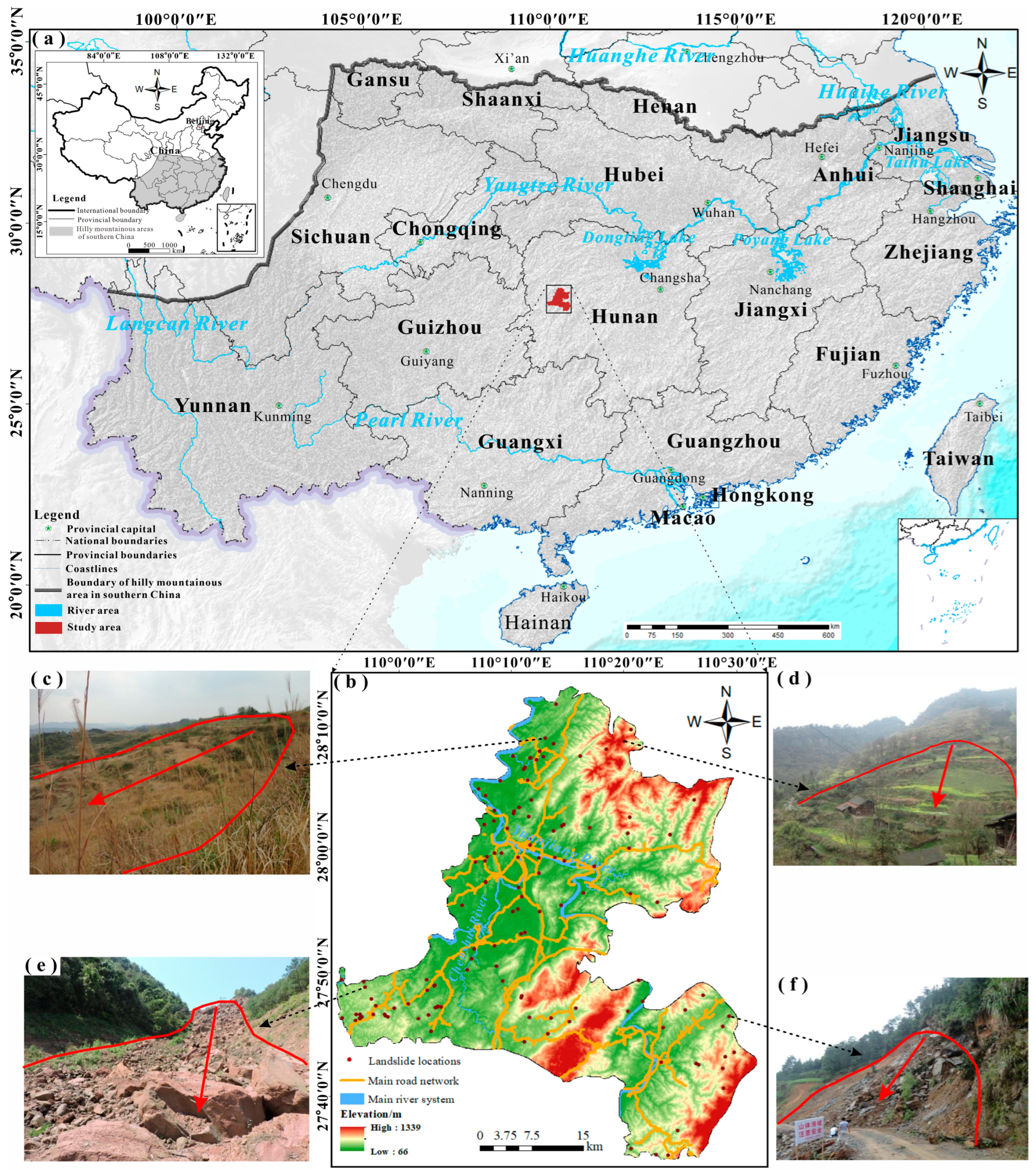
2.1. Overview of the Study Region and Source

Chenxi County spans an area of roughly 1976.81 km² and is located in Huaihua City Hunan Province among the hilly and mountainous regions of southern China. It is not only a part of the complex structural stress zone that separates the Dongting Lake Plain from the Yunnan–Guizhou Plateau, but also a part of the middle–low mountainous region in western Hunan (Figure 1a), which is one of the key geological disaster-prevention areas with a fragile ecosystem in China [32,33]. This area is also a geological-disasters-concentrated region with undulating terrain, diverse geological environment, and changing climate over time and space [6,34].

The elevation generally ranges from 200 to 300 m, with topographically higher altitudes in the southeast and lower altitudes in the northwest. The prominent landform consists of mountains and hills with intervening plains. Mountains, hills, and plains account for 61%, 36%, and 3% of the county in total, respectively (Figure 1b). The stratigraphic age extends from the Qingbaikou system to the Quaternary system, excluding the Silurian system, and all outcrops in the region are sedimentary rocks.

The southeast monsoon significantly affects the humid subtropical monsoon climate of the county. There are four distinct seasons and a warm climate with concentrated and plentiful summer precipitation. According to Chenxi County Meteorological Station and Chenxi County Hydrological Bureau data, the annual average temperature is 17.0 °C. The mean yearly precipitation and evaporation are 1404.9 mm and 1301.2 mm, respectively. The maximum recorded amount of daily rainfall is 235 mm. Yuanjiang River and the Chenshui River converge in the county (Figure 1b).

In recent decades, under the dual effects of extreme weather such as heavy rainfall and intense human engineering activities, a higher frequency of geohazards take place in the county. With the increasingly severe situation of geological disaster prevention in the study area, attaining a higher accuracy of regional landslide susceptibility assessment and prediction is urgent.

2.2. Data Preparation and Analysis

2.2.1. Landslide Inventory

Since the compilation of landslide records provides the basic data, its accuracy and integrity are critical and vital to susceptibility assessment and prediction. After analysing the historical landslide records, satellite images, and field investigations, Chenxi County was ultimately found to have 127 landslides (Figure 1b), the bulk of which were small to medium in size. The study area has seen a frequent occurrence of geohazards in recent years. Notably, in 2014, 53 landslides were induced by the summer rainstorm. In terms of material composition, the accumulation landslides (Figure 1c,d) account for 75.6% of all landslides; bedrock landslides (as shown in Figure 1e) come in second with 14.2%; and rubble soil landslides (as shown in Figure 1f) occur the least, accounting for only 10.2%. Out of all the historical landslides, the majority of them were triggered by rainfall, making up 86.7% of the total. In total, 9.4% of landslides result from the combination of the influences of rainfall and human activities, while just 3.9% of landslides are due to either weathering or human activities independently. Regarding slope structure, the most common are longitudinal and oblique slopes, accounting for 45.7% and 29.1% of all landslides. The second slopes are the reverse and lateral slopes, accounting for 11.8% and 10.2%, respectively. The gentle slope is the least common type, only contributing 3.2%.

In the landslide modelling process, ArcGIS 10.2 is utilised to determine the centroid of the landslide polygon, which indicates the actual landslide locations, as most of them in the study region are less than 10,000 m³. Many landslide investigations have demonstrated the viability of this approach and its ability to streamline landslide data efficiently [35,36,37]. Hence, each landslide has been depicted pointwise in this study.

2.2.2. Landslide Impact Factors

Landslides develop as a consequence of the interplay between internal and external causes. The selection of impacting elements is vital to predicting landslide susceptibility due to the diverse range of impact factors that can influence landslides and the complicated nature of their formation mechanism [38,39,40]. Nevertheless, there have been no set rules for selecting impact factors. This study introduces 21 factors contributing to landslides to create an index system for assessing susceptibility. These factors were derived from five main aspects: geology, hydrology, topography, meteorology, human activities, and geographic environment. The selection of these factors was primarily on the basis of field investigations as well as the specific characteristics herein. Topographic elements include elevation, slope angle, slope aspect, slope curvature, plane curvature, profile curvature, terrain roughness, terrain ruggedness index (TRI), topographic position index (TPI), and relief degree of land surface (RDLS). Geological variables encompass the proximity to faults (e.g., dip, strike, etc.) and the classification of rock formations for engineering purposes. Meteorological and hydrological parameters include the proximity to rivers, amount of rainfall, topographic wetness index (TWI), and stream power index (SPI). Human activities are affected by impact factors, e.g., the proximity to highways, the density of the population, as well as the types of land utilisation and land cover (LULC). Geographic environmental elements include soil type and normalised-difference vegetation index (NDVI).

The Digital Elevation Model (DEM) was utilised in this study to access topographic information, e.g., elevation, slope angle, and slope curvature. Hydrological data, such as SPI and TWI, were collected using the ASTER satellite, which has a resolution of 30 m. The geological mapping, which was extracted from the China Geological Archives (accessible at http://www.ngac.cn/, accessed on 2 April 2024), has a scale of 1:50,000 and was used to access information on fault layers and engineering rock groups. The information regarding rivers and roads was acquired from the Open Street Map (accessible at http://www.openstreetmap.org/, accessed on 6 April 2024). The soil type and land cover data were acquired from the Resource and Environmental Science Data Centre of the Chinese Academy of Sciences (accessible at http://www.resdc.cn/, accessed on 2 April 2024). The mean yearly rainfall data were acquired from the online database offered by the China Meteorological Data Network (accessible at http://data.cma.cn/, accessed on 2 April 2024). The population density information was acquired from the United States National Aeronautics and Space Administration (NASA). The NDVI was computed using Landsat 8 data, resulting in a resolution of 30 m. The comprehensive factors contributing to landslides can be observed in

Table 1. All data sources and factor evaluation systems in the study region.

Groups	Factors	Descriptions	Data Sources
Topography	Elevation	ASTER GDEM V2, 30 m resolution	http://www.gscloud.cn/ (accessed on 6 April 2024)
	Slope	Obtained by using SAGA 7.0, 30 m resolution	Extracted by DEM
	Aspect
	Curvature
	Plane curvature
	Profile curvature
	Terrain roughness
	TRI
	TPI
	RDLS
Geology	Distance to faults	Vector data	http://www.ngac.cn/ (accessed on 2 April 2024)
	Engineering rock group
Meteorology and hydrology	Distance to rivers	Vector data	http://www.openstreetmap.org/ (accessed on 2 April 2024)
	Rainfall	Interpolated from the online database, 1985–2020	http://data.cma.cn/ (accessed on 2 April 2024)
	SPI	Obtained by using SAGA 7.0, 30 m resolution	Extracted by DEM
	TWI
Human activities	Distance to roads	Vector data	http://www.openstreetmap.org/ (accessed on 6 April 2024)
	Population density	Reclassify to 30 m resolution	https://www.nasa.gov/ (accessed on 6 April 2024)
	LULC	30 m resolution	http://www.resdc.cn/ (accessed on 2 April 2024)
Geographic environment	Soil types	Reclassify to 30 m resolution	http://www.resdc.cn/ (accessed on 2 April 2024)
	NDVI	Landsat 8, 30 m resolution	https://www.gscloud.cn/ (accessed on 6 April 2024)

.

2.3. Assessment Units

Most recent studies have commonly employed grid units, administrative units, slope units, and geomorphic units as the assessment units for landslide susceptibility prediction [41]. According to Yang et al. [42], grid units are generally more effective for complex calculations and simulation processes than other units. Thus, we used grid units as the primary evaluation units in this study. Given the size of the research region and the computational complexity, we also consulted the empirical formula [43] for determining the grid cell size:

$$G_s=7.49+6\times {10}^{-4}S-2\times {10}^{-9}{S}^2+2.9\times {10}^{-15}{S}^3$$

(1)

where $G_s$ represents the appropriate grid size, and $S$ is the denominator of the map’s digital scale.

In our study, the scale of detailed survey is 1:50,000, the optimal grid cell is calculated as 32.853 m, which is convenient for data analysis. This study uses 30 m × 30 m grid cells as the minimum evaluation unit for a total of 2,191,610 grid cells.

3. Methodology

3.1. Landslide Susceptibility Modelling Process

This study’s methodology flowchart is displayed in Figure 2. The process comprises six main steps: (I) Acquire the updated landslide datasets to form the landslide inventory. (II) Establish the impact factors system. (III) Screen the impact factors by eliminating the factors with high correlation through multicollinearity detection. (IV) Construct the modelling dataset by merging the recorded landslides and the same number of selected non-landslide samples and set the ratio of training dataset to validation dataset as 7:3. (V) Predict landslide susceptibility by applying 12 prediction models. (VI) Validate and compare the prediction models performances by various evaluating indexes.

3.2. Optimised Sampling Approach for Non-Landslide Samples

Landslide deformation and instability processes are affected by coupled factors, e.g., geology, hydrology, topography, meteorology, human activities, as well as geography, because the environment feature space contains many factors that influence the evolution and deformation of landslides. If a grid or point (x, y) is more distinctive to the environmental similarities of the existing landslides, it is less likely to be prone to landslides. Thus, its selection as a non-landslide sample is more reliable. Hence, a core idea of considering the reliability of non-landslide data based on environmental similarity is introduced. Meanwhile, the CF model, a conventional statistical method, reflects the probability of future geohazards based on the same geological circumstances [44]. Therefore, a novel method that fuses the reliability of non-landslide data and the CF value is proposed to optimise the selection of negative samples. The flow chart of the procedure is shown in Figure 3.

The implementation of the optimised sampling method involves three primary processes. (I) Screened impact factors were divided into two types: continuous and discrete. Subsequently, the frequency ratio model and kernel density estimation were utilised to determine the environmental similarity between a specific impact factor and the standard value for the existing landslides associated with that factor. Subsequently, the reliability of non-landslide samples was computed for each grid, considering the total environmental similarity. (II) The CF value for each grid was calculated using the formula of the certainty factor model. (III) Non-landslide samples were chosen from high- and very-high-overall score zones. This selection process ensures that the dependability of non-landslide samples and the CF value are combined and standardised. Here are the details of these procedures.

3.2.1. Reliability of Non-Landslide Samples

Environmental Similarity of the Discrete Factors

Considering the discrete impact factors, the environmental similarity between a single factor and the typical value for the existing landslides under the factor was calculated via the method of frequency ratio. By quantifying the frequency of sample classification, we can judge the categories of certain impact factors that prominently impact the landslide incidences. The mentioned statistical model is frequently used to analyse two variables simultaneously [45,46,47]. This work utilises the method of frequency ratio to statistically describe the correlation between every impact factor and the frequency of landslide occurrence. The formula for this correlation is given below:

$$F{R}_{i,j}={\displaystyle \frac{F_{i,j}/A_{i,j}}{{\displaystyle {\sum }_{j=1}^m{F}_{i,j}/A}}}$$

(2)

where F_i,j represents the occurrence frequency of the landslides in category j under the ith factor; A_i,j is the area of the category j under the ith factor; m stands for the number of the categories of the ith factor; and A is the total area of the investigated region.

To obtain the environmental similarity between the category j of the ith factor and the typical category of landslides occurring under the ith impact factor, we use the following expression:

$$S_{i,j}={\displaystyle \frac{F{R}_{i,j}}{\max (F{R}_{i,j})}}$$

(3)

Environmental Similarity of the Continuous Factors

For the continuous impact factors, the estimation of kernel density was applied to the determination of the environmental similarity between the grids and existing landslide grids [48,49]. Foremost, suppose there are n cases of landslides under different impact factors x₁, x₂, x₃, …, x_n. Thenceforth, the function of probability density expressing the correlation between the impact factor x and frequency of landslide occurrence is given as follows [50]:

$$f(x)={\displaystyle \frac{1}{nh}}{\displaystyle {\sum }_{i=1}^{n}k(\frac{x-x_i}{h}})$$

(4)

where k is the kernel estimation formula, h stands for the bandwidth, which determines the smoothness and shape of the estimation curve for kernel density, and x − x_i is the gap between the value of the impact factor x and the value of the impact factor x_i at the actual location of the existing landslide. In this research, we utilise a commonly employed Gaussian kernel estimation formula to determine the estimation curve for the kernel density and compute the bandwidth h. The formula frequently used for the purpose is provided as follows:

$$f(x)={\displaystyle \frac{1}{nh}}{\displaystyle {\sum }_{i=1}^{n}k(\frac{x-x_i}{h}})={\displaystyle \frac{1}{\sqrt{2\pi }}}{e}^{-{\displaystyle \frac{{(x-x_i)}^2}{2h^2}}}$$

(5)

$$h=\sigma {({\displaystyle \frac{4}{3n}})}^{0.2}$$

(6)

where σ stands for the standard deviation for a series of values of the impact factor x where n landslides are located.

The environmental similarity of the continuous impact factors can be obtained by normalising the f(x), and the normalisation expression is as follows:

$$S_x={\displaystyle \frac{f(x)}{f_{\max }(x)}}$$

(7)

where f(x) stands for the function of probability density expressing the correlation between the frequency of landslide occurrence and the impact factor x; f_max(x) indicates the maximum value for f(x).

Comprehensive Environmental Similarity

By integrating the similarity of an impact factor to the typical value of landslide occurrence under the impact factor, the comprehensive environmental similarity of the typical landslide can be measured, and the formula is as follows:

$$C{S}_{x,y}=f(S_1,S_2,\dots ,S_k,\dots S_n)$$

(8)

where CS_x,y is the comprehensive similarity of the environment in the grid at (x, y); S_k is the environmental similarity between the kth impact factor and the typical value of landslide occurrence under this factor; f is the integration function, and the mean function, which is a commonly used function, is selected in this study.

Calculation of Reliability of Non-Landslide Samples

According to the cognition that “samples of the same type are close to each other in the environmental features, and samples of different types are separated”, the more dissimilar the area is to the landslide samples in the environmental features, the more likely it is to be a non-hazard area, that is, a high-reliability area for non-landslide datasets. The reliability of non-landslide data might be achieved by the subsequent expression:

$$R_{x,y}=1-C{S}_{x,y}$$

(9)

where CS_x,y is the comprehensive similarity of the grid at (x, y); R_x,y is the reliability that this grid is selected as a non-landslide sample.

3.2.2. Calculation of the CF Value

The certainty factor (CF) model is a probabilistic function introduced by Shortliffe and Buchanan in 1975 [51]. Despite the simplicity of the model evaluation approach, it achieves a high level of accuracy. To achieve better precision and accuracy at a high level, it is necessary that the landslides that have already happened and the potential future geohazards occur under identical conditions. The formula to compute CF could be given below:

$$CF=\left\{\begin{array}{l}{\displaystyle \frac{P{P}_a-P{P}_s}{P{P}_s(1-P{P}_a)}}(P{P}_a<P{P}_S)\\ {\displaystyle \frac{P{P}_a-P{P}_s}{P{P}_s(1-P{P}_a)}}(P{P}_a\ge P{P}_S)\end{array}\right.$$

(10)

where PPs represents the probability of historical landslides occurring throughout the entire investigated region, which is defined as the ratio of the number of historical landslides to the total area of this region, and PPa is the conditional probability of landslides in the impact factor classification a, which can be determined as the ratio of the number of landslides in classification a to the classification area.

The CF values vary between –1 and 1. If the values range from 0 to 1, it indicates a susceptibility to landslides in this particular environment. A greater value of CF indicates a higher susceptibility of the grid to landslides. Conversely, if the CF values range from –1 to 0, the occurrence of landslides in this environment is improbable.

3.2.3. Unified Scalar Overlay Approach

The reliability of negative samples is capable of characterising environmental dissimilarity to typical landslides in the given region. Landslide susceptibility zoning on the basis of the CF model can guarantee higher probabilities of selecting negative samples. To minimise subjectivity in evaluating a single model and to incorporate valuable information from various models, we incorporated the reliability of negative samples with the CF model to improve the quality of non-landslide datasets. This could be achieved by utilising the following formula:

$$x_{norm}={\displaystyle \frac{x_i-\min \left\{x_1,x_2,\dots ,\left.x_n\right\}\right.}{\max \left\{x_1,x_2,\dots ,\left.x_n\right\}\right.-\min \left\{x_1,x_2,\dots ,\left.x_n\right\}\right.}}$$

(11)

$$OS=R(0,1)+1-CF(0,1)$$

(12)

where x_i refers to the raster value in the resulting map (the reliability of negative samples or the CF); the value after normalisation is represented as x_norm; min{x₁, x₂, …, x_n} and max{ x₁, x₂, …, x_n} represent the minimum and maximum values among all raster values. The normalisation outcomes of the reliability of the negative sample layers and the CF value layers are indicated by R(0, 1) and CF(0, 1), accordingly. The optimal sampling method value (OS) is derived from the normalised fusion of the reliability of the negative sample layers and the CF value layers.

3.3. Machine-Learning Model

3.3.1. Random Forest Model

The random forest (RF) algorithm, which is a machine-learning technique, operates by randomly selecting a subset of inventory and generating numerous binary decision trees through bootstrapping. Subsequently, these trees are combined to calculate a categorisation or prediction [52,53,54,55]. The decision tree algorithm was employed to train multiple samples retrieved from the initial datasets, with replacement, and, subsequently, these decision trees are aggregated. The ultimate categorisation outcome is determined by the one that receives the highest number of votes. The operational idea of the RF method is illustrated in Figure 4. The process can be described in the following three steps: (I) Construct n decision trees via the bootstrap method, which involves arbitrarily selecting n new sample sets with replacement from the original training dataset. (II) For each re-sampling, select a random set of features and use them to construct n decision trees. (III) Integrate the generated trees to create an RF, which is then used to categorise newly acquired data. The final classification outcomes are determined through decision tree voting. When dealing with intricate data, the RF model demonstrates outstanding accuracy and robust reliability by using significant variabilities across the individual trees for classification tasks [56]. The current work utilised the RF model for the evaluation of the landslide susceptibility prediction when taking the benefits mentioned above into account.

3.3.2. Support Vector Machine Model

The support vector machine (SVM) is a non-parametric machine-learning algorithm that takes advantage of kernels to perform classification, regression, and prediction tasks by creating a collection of hyperplanes in infinite-dimensional space [57,58,59,60]. SVM excels at addressing linear and non-linear classification and regression issues by providing complicated and reliable solutions. SVM modelling differs from other discriminant-type methods by utilising an optimum linear hyperplane to distinguish data patterns. The schematic diagram illustrating the principle of SVM modelling is depicted in Figure 5. Margin refers to the measurement of the distance between the hyperplane and the closest sample point. The classifier’s ability to generalise improves as the margin increases [61]. Therefore, the SVM aims to determine the ideal hyperplane, i.e., the one that maximises the margin. Support vectors are the locations on the hyperplane that determine the classification border and are located on each side of the margin. Hence, the SVM performance is mainly dependent on the adjustment of its hyperparameters. The three primary SVM hyperparameters are C, γ, and kernel type, where parameter C dominates the balance between the decision boundary and accuracy by imposing a penalty for each incorrectly classified data item, and parameter γ is in certain kernel types that are linked to C, and the kernel type is responsible for mapping the inventory into a feature space, as discussed earlier. When the value of γ is high, the influence of C is minimalised. If γ is modest, C has a comparable impact on the model as it does on a linear model.

3.3.3. Back Propagation Neural Network Model

The back propagation neural network (BPNN) is a multilayer network algorithm capable of efficiently mapping multidimensional functions and accurately classifying complicated patterns [62]. The BPNN architecture used in the study is schematically plotted in Figure 6. The system comprises three layers: input and output layers, as well as a hidden layer. Each layer is linked to the surrounding layers using activation functions. During the computation, each neuron in a layer utilises the output value of the neuron in the former layer as input. It then processes this input value based on the weights and thresholds and outputs the computed result to the neuron in the next layer [63,64,65,66]. The BPNN model has the ability to extract accurate conclusions and calculate the underlying rules from vast amounts of ambiguous and intricate datasets in a dynamic environment. The data utilised in the susceptibility assessment procedure predominantly capture qualitative rather than quantitative information pertaining to landslides. By analysing this ambiguous information, precise assessment findings can be achieved. Landslide susceptibility evaluation is primarily an investigation that focuses on identifying and analysing patterns. The BPNN model is extensively used in non-linear modelling, pattern recognition, and pattern classification thanks to its ability to represent any continuous functions with any degree of accuracy.

3.3.4. Heterogeneous Ensemble Machine-Learning Model

A heterogeneous ensemble machine-learning model refers to a combination of diverse machine-learning algorithms through different strategies to build a prediction model with better performance. The individual algorithms that constitute ensemble learning are called baseline models or base learners. To train an ensemble learner model, it is necessary to train several different base models first and then train the ensemble model with the output of these base models as input to obtain a final output. Because it can ensemble different types of classifiers, heterogeneous integrators can realise the complementary advantages and disadvantages of different base models to further eliminate errors and improve prediction accuracy. In addition, heterogeneous integrators can achieve heterogeneity by integrating a wide range of baseline models, hence avoiding the difficulty of model selection to some extent. Heterogeneous ensemble models mainly include stacking, blending, and weighted average algorithms. In the study, the stacking algorithm was utilised to complete the ensemble machine learning.

Stacking ensemble machine learning, a classic heterogeneous ensemble learning algorithm, applies a meta-model to combine various baseline models to create a new model that produces predictions with higher precision [67,68,69]. As shown in Figure 7, the modelling dataset is first separated into the training and validation sets as 7:3. Next, the modelling dataset is input into several baseline models. The prediction information are integrated into a new one, which is then used by the meta-model to output the final results [70]. The study employs the logistic regression (LR) method as the meta-model and combines the baseline models RF, SVM, and BPNN to form a heterogeneous ensemble machine-learning model known as the stacking ensemble model.

Logistic regression (LR), an extension of diverse regressions, is a predictive analysis in which the events are considered the dependent variables, while the predisposing factors are treated as the independent variables [71]. The discriminant analysis enables logistic regression to exam predictor variables of diverse forms, including discrete, dichotomous, and continuous variables, which makes it possible to create non-linear models [72]. A benefit of LR over linear and log-linear regression is that it does not necessitate a normality condition. To choose the “best” predictor used in the model step by step, there are multiple methods available in the LR procedure. The LR equations are listed below:

$$f(x)=c_0+c_1{x}_1+\dots +c_n{x}_n$$

(13)

$$f(x)=\log it(P)=\ln \left[{\displaystyle \frac{P}{1-P}}\right]$$

(14)

$$P={\displaystyle \frac{1}{1+e^{-f(x)}}}={\displaystyle \frac{1}{1+e^{-(c_0+c_1{x}_1+\dots +c_n{x}_n)}}}$$

(15)

where x₁, …, x_n are referred to as predictor variables, and f(x) represents a linear function combining these predictor variables, which stands for a linear relationship. Parameter c₀ is the model intercept, and parameters c₁, …, c_n are the coefficients of regression, which ought to be estimated. P is the occurrence likelihood of an event (a landslide), and 1 − P is the likelihood that an event will not occur. The log it(P) is the symbol for the function f(x). When the values of f(x) increase, the probability P also rises. The probability of change increases in response to the predictor variable, and vice versa, according to a positive sign.

3.4. Validation of Landslide Susceptibility Prediction

The confusion matrix is often applied to assess the precision of model predictions for geohazards, such as landslides, which are typical binary classification issues. In this study, the predicted value was evaluated using a threshold of 0.5. It is considered a landslide (assigned 1), provided that the predicted value is >0.5. Otherwise, it should be classified as non-landslide data (assigned 0). We selected the following formulas to define precision (PRE), accuracy (ACC), recall (SST), and F1-score (FS) as the assessment metrics for our model based on the confusion matrix.

$$PRE={\displaystyle \frac{TP}{TP+FP}}$$

(16)

$$ACC={\displaystyle \frac{TP+TN}{TP+FP+TN+FN}}$$

(17)

$$SST={\displaystyle \frac{TP}{TP+FN}}$$

(18)

$$FS={\displaystyle \frac{2TP}{2TP+FP+FN}}$$

(19)

where TP indicates that both the predicted and actual values are positive; TN is utterly opposite to TP; FN denotes that the predicted and actual values are less than 0 and over 0, respectively; FP is totally opposite to FN [73]. The values of PRE, ACC, SST, and FS fall into a range between 0 and 1. The PRE value reaching closer to 1 means a higher proportion of accurately predicted landslide samples. Similarly, the ACC value approaching closer to 1 signifies a higher overall modelling accuracy. Additionally, when SST turns closer to 1, it shows a greater predictive capacity of the model for landslides. FS is an index indicating a combination of precision and recall. A higher value of FS demonstrates a more substantial output effect of the model [74,75].

When dealing with issues in terms of dichotomous classification, in addition to metrics, e.g., recall, accuracy, precision, and F1-score, the receiver-operating characteristics curve (ROCC) is commonly employed as a key indicator in modelling success. The ROCC effectively assesses the predictive capability of a model by assessing its performance against a given probability threshold [76]. The x-axis of the ROCC corresponds to the false positive rate or specificity, while the y-axis corresponds to the genuine positive rate or sensitivity. The AUC in the range of 0.5~1 represents the area under the ROCC. Models that exhibit higher AUCs demonstrate superior performance.

4. Results and Analysis

4.1. Impact Factors Classification and Frequency Ratio

In this paper, the continuous factors in the evaluation system include elevation, slope angle, slope aspect, slope curvature, profile curvature, plane curvature, terrain roughness, TPI, TRI, TWI, RDLS, SPI, NDVI, rainfall, distance to rivers, distance to faults, distance to roads, and population density. The natural fracture method is adopted to carry out classification. Discrete factors include engineering rock groups, soil types, LULC, etc., and the natural grouping approach is adopted for classification. The outcomes from the classification are depicted (see Figure 8).

Statistical models, specifically the FR and CF models, are employed to compute the frequency ratio and determination coefficient values for each impact factor across various classifications. This allows us to determine the degree of impact that each category of impact factor imposes on landslide susceptibility. These results then serve as input data for the model to predict landslide susceptibility. Frequency ratios and determination coefficient values of each factor are displayed in Figure 9.

4.1.1. Topography

Topographic factors are the basic variables that influence the distribution of landslides, and areas with surface fluctuation and significant fragmentation are more susceptible to landslides [77].

Elevation is a measure commonly applied to evaluate the landslide probabilities. Landslides in mountainous and hilly environments are influenced via various external conditions that are directly associated with elevations, e.g., precipitation, vegetation cover, and human activity. The landslide distributions in the investigated region are primarily concentrated in areas having low mountains, hilly, as well as valley slopes, where the elevation is under 350 m from the sea datum. These areas account for 88.98% of the total landslide numbers. FR values of elevation factors achieve their highest within the range of 66 to 200 m, suggesting a high susceptibility to landslides (see Figure 8a and Figure 9a).

The slope angle is a vital factor that directly impacts the stress field’s distribution and rainfall’s infiltration process, determining slope stability. The majority of landslides are found in slopes with an inclination below 30°, and the occurrence likelihood of landslides is highest when the slope is between 20° and 30° (see Figure 8b and Figure 9b).

The slope aspect is crucial in the determination of the amount of surface water runoff and the intensity of solar radiation, which affects the slope stability and deformation in turn [78]. The probabilities for triggered landslides are greater in the southeast and southwest directions in the county, as shown in Figure 8c and Figure 9c. Combined with the local geological environment, it indicates that the slopes in the above two aspects have greater evaporation and less soil moisture, shallower and sparser vegetation roots, and larger daily temperature changes, which are more likely to cause rock weathering, hence the evolution and development of landslide being affected.

Three geometric factors of a slope, e.g., curvature, profile curvature, and plane curvature, mainly control surface runoff and erosion and indeed have influences on the occurrence of landslides in turn [79]. The highest number of existing landslides and the FR values are shown in the investigated areas when the curvature is 0~1.0 (see Figure 8d and Figure 9d), the plane curvature is 0~0.5 (see Figure 8e and Figure 9e), and the profile curvature is 0~0.5 (see Figure 8f and Figure 9f), indicating that the convex slopes are more prone to landslides. TRI is a measure of surficial morphology calculated by comparing the terrestrial surface area to the corresponding projected area of a given region. The probability of landslides is highest when the TRI falls between 1.0 and 1.05 in the entire county (see Figure 8h and Figure 9h). The proportion of landslides occurring when the terrain roughness is less than 38 m is 96.06%. Additionally, the FR value reaches its maximum when the terrain roughness falls into the range of 13 to 25 m (see Figure 8g and Figure 9g). When TPI ≤ –1 and TPI ≥ 1 in the research region, the FR value increases, indicating that landslides are more developed and distributed in ridge areas or valley slopes (see Figure 8i and Figure 9i).

RDLS is an important factor that quantifies the variation between the minimum and maximum elevations in a designated region, which has a prominent impact on the landslides occurrence [80]. Within the investigated region, the proportion of landslides is 95.28% for RDLS ranging from 0 to 20 m (see Figure 8j and Figure 9j).

4.1.2. Geology

The geological setting has exerted effects on the genesis of landslides, including impact factors: the distance to faults and engineering rock groups. The effects of faults on rock and soil include interlayer dislocation, structural breakage, etc. Cracks develop near faults, and rock mass is broken, making it easy to form loose residual slope deposits obversely attached to bedrock and provide the necessary material for developing sliding slopes. Engineering-rock groups are the basic material condition for controlling landslide occurrence since they directly influence the magnitude and type of such disasters. As the formation integrity worsens, the strength of geotechnical engineering decreases, the geological environment becomes more unstable, and the likelihood of slope instability increases. The closer the distance from the faults in the research region, the greater the likelihood of landslides occurring (see Figure 8k and Figure 9k). The engineering-rock groups that are prone to landslide include medium-dense clay and gravel and soft to moderately hard siltstone, sandstone, and mudstone. The number of landslides and FR value are high in the distribution of the above two engineering-rock groups (see Figure 8l and Figure 9l).

4.1.3. Human Engineering Activities

The extensive and swift expansion of human engineering activities, including agricultural irrigation, mineral exploitation, and transportation construction, has significantly disrupted the original stable state of slopes, leading to a substantial increase in landslides. Crucial indexes, e.g., the population density, distance to roads, and LULC, are typical symbols of human activities. Approximately 77.17% of the landslides in the investigated region are concentrated in an area within 2000 m of road systems. The likelihood of triggering landslides steadily increases as the distance to roads decreases, as shown in Figure 8m and Figure 9m. Landslides primarily occur in regions characterised by low-elevation mountains, valleys, and other locations with a population density in a range of 96~248 people/km². However, under the background of urbanisation, due to the limitation of construction land and the intensification of engineering activities such as building houses by cutting slopes, the probability of landslides is the largest in the area of 409~762 people/km² (see Figure 8n and Figure 9n).

4.1.4. Meteorology and Hydrology

Meteorological and hydrological conditions such as rainfall and river-flushing will significantly alter the slope’s internally stable state, which is a key factor triggering landslide initiation. In the research region, 74.80% of the landslides were found to occur at a distance of 500 m from the rivers. The landslide possibilities steadily increased as the distance to the rivers decreased (see Figure 8p and Figure 9p). Landslides are mainly distributed in areas with TWI ≤ 10, accounting for about 92.13% of the total number, while the TWI with the highest probability of slope occurrence is between 0 and 5 (see Figure 8s and Figure 9s). The grading findings indicate that the majority of the sliding slopes are concentrated in the region with an SPI value ranging from 1.37 to 2.83. These slopes account for approximately 49.61% of the total number of sliding slopes (see Figure 8r and Figure 9r). In the study region, the landslide frequency and FR values are both high, with precipitation between 1284~1343 mm/year (see Figure 8q and Figure 9q).

4.1.5. Geographic Environment

Geographic environmental factors, including NDVI and soil types, are significant factors that cannot be ignored in terms of affecting slope stability. The higher the NDVI, the lower the effect of precipitation-induced infiltration on slopes. Meanwhile, the root system of plant cover has a certain strengthening effect on a slope. The bare vegetation on the surface of the ground is less covered, and the slope is extremely vulnerable to hydraulic encroachment and erosion, which leads to landslides. Different types of soil exhibit various physical and chemical properties, fundamentally determining the source basis of landslide formation. The number of existing landslides with NDVI between 0.6 and 0.7 accounts for 39.37% of the study area. When the NDVI is 0.15~0.45, the FR values are the highest, indicating the possibility of forming landslides is greatest (see Figure 8u and Figure 9u). In total, 62.21% of the landslides are distributed in red soil and yellow soil, and the probabilities of landslide development in brown soil are the highest (see Figure 8t and Figure 9t).

4.2. Multicollinearity Detection among Factors

The multicollinearity of selected dominant factors will lower the model’s prediction accuracy and probably cause the model to fail. Thus, it is essential to detect the independence of all the impact factors through correlation analysis and collinear diagnosis before machine learning. Most academics frequently employ Pearson correlation coefficients (PCCs), tolerance (TOL), and variance inflation factor (VIF) for screening factors. It is generally believed that when PCCs > 0.5, the two factors have a relatively high correlation; when TOL < 0.1 and VIF > 10, the factor does not have multicollinearity [81,82,83].

As shown in

Table 2. VIF and TOL of all the impact factors.

Impact Factors	TOL	VIF	Impact Factors	TOL	VIF
Elevation	0.485	2.062	Distance to Faults	0.718	1.393
Slope angle	0.250	3.502	Engineering-Rock Group	0.669	1.494
Slope aspect	0.651	1.536
Slope curvature	0.509	1.966	Distance to Roads	0.667	1.495
Plane Curvature	0.712	1.404	Population Density	0.774	1.292
Profile Curvature	0.714	1.401	LULC	0.364	2.750
Terrain Roughness	0.245	4.896	Distance to Rivers	0.736	1.357
TRI	0.317	4.398	Rainfall	0.733	1.362
TPI	0.745	1.342	SPI	0.436	2.291
RDLS	0.152	4.972	TWI	0.379	2.637
NDVI	0.375	2.665	Soil types	0.727	1.376

, the VIF and TOL of the 21 impact factors in our study satisfy the threshold conditions for non-collinearity. As depicted in Figure 10, the PCCs between the following groups of factors, namely terrain roughness and slope angle, TRI and slope angle, TRI and terrain roughness, RDLS and slope angle, and RDLS and TRI, are >0.5, indicating a series of high correlation, while the correlations between the rest impact factors are relatively low. Therefore, the factors of terrain roughness, TRI, and RDLS with the highest VIF values in the above two groups of factors are eliminated. The remaining 18 factors were substituted into the baseline models and the hybrid models to develop landslide susceptibility prediction in the county.

4.3. Sample Selection Results

A total of 127 positive samples (existing landslides) have been acquired from the landslide inventory of the research region. In the study, three methodologies adopted to choose 127 negative samples (non-landslide samples) are as follows: (1) Random sampling (RS) method: create a buffer zone with a radius of 500 m centred on the known landslide points, and the negative samples were randomly selected from outside of it (see Figure 11a). (2) Certainty factor-based (CF) sampling method: employ the CF model to calculate the CF value for each grid and generate the landslide susceptibility zoning; then, the negative samples were picked randomly from the very low and low susceptibility zoning areas (see Figure 11b). (3) OS method: obtain a comprehensive score by fusing the reliability of the non-landslide samples with CF values for all grids; then, the negative samples were picked up from those regions with very-low and low corresponding values at random (see Figure 11c).

4.4. Machine Learning Parameter Settings

In our study, the Sklearn library of Python language is used for machine-learning model construction, and parameters are optimised by learning curve and grid search. The parameters used by each baseline models are set as follows: When the number of random forest model classifiers increases to 200, the maximum depth of the decision tree reaches at 10, and the score reaches a peak and then becomes stable; the kernel function of the support vector machine model is a linear kernel function, and the penalty coefficient is 0.1. In the BP neural network model, the number of neurons in the hidden layer is 100, the activation function is Tanh, the optimizer is Adam, and the regularisation parameter alpha is 0.001.

4.5. Prediction of Landslide Susceptibility

To evaluate the OS strategy’s reliability and validity for the selection of non-landslide samples and the heterogeneous ensemble machine-learning model’s generality and resilience proposed in our study. We selected negative samples based on the RS, CF, and OS methods, respectively. After inputting the three abovementioned sample sets, the likelihood of landslide occurrence for all grids was determined through the baseline models (RF, SVM, BPNN) and the heterogeneous ensemble stacking model. Next, we categorised the landslide susceptibility into five classifications using the natural fracture technique: very low, low, moderate, high, and very high. Then, the landslide susceptibility maps generated by the RS–RF, RS–SVM, RS–BPNN, RS–Stacking; CF–RF, CF–SVM, CF–BPNN, CF–Stacking; OS–RF, OS–SVM, OS–BPNN and OS–Stacking models will be obtained in sequence (see Figure 12). These susceptibility maps from the 12 prediction models exhibit almost visually identical patterns, with the majority of high-prone areas located in the southeastern and northeastern part. When comparing the 12 susceptibility maps with the locations of natural landslides, it is observed that the distribution of landslides is generally accordant. This is because the areas have complex geological structures, relatively soft technical lithologies, and traversing river systems. In addition, the areas are increasingly impacted by human engineering endeavours, such as the construction of transportation facilities and house building via cutting slopes, heightening the risk of triggering landslides. However, it is visible that the high-prone zone yielded using the stacking ensemble model is more concentrated than that by the other baseline models. Furthermore, there is more clumping in high-prone regions when applying the OS method for selecting the non-landslide data under the same machine-learning model.

5. Validation of Prediction Models

Evaluating the prediction models is crucial for determining landslide susceptibility outcomes. The evaluation indexes, including accuracy (ACC), precision (PRE), F1-score (FS), and recall (SST), along with AUC and ROCC, were applied to conduct a comparison of the 12 prediction models performances.

According to those evaluation indexes listed in

Table 3. Model prediction performance result.

Models	Precision	Accuracy	Recall	F1-Score
RS–RF	0.767	0.755	0.768	0.761
RS–SVM	0.736	0.721	0.742	0.723
RS–BPNN	0.739	0.722	0.743	0.726
RS–Stacking	0.778	0.764	0.789	0.772
CF–RF	0.903	0.892	0.905	0.897
CF–SVM	0.878	0.865	0.882	0.866
CF–BPNN	0.881	0.869	0.884	0.874
CF–Stacking	0.911	0.898	0.915	0.902
OS–RF	0.924	0.901	0.927	0.908
OS–SVM	0.892	0.879	0.896	0.881
OS–BPNN	0.898	0.885	0.902	0.890
OS–Stacking	0.933	0.906	0.936	0.912

, the values of accuracy, precision, F1-score, and recall by the OS–RF, OS–SVM, OS–BPNN, OS–Stacking, CF–RF, CF–SVM, CF–BPNN, and CF–Stacking models all exceeded 0.85, with the OS–Stacking model ranking highest, with a value over 0.9. In contrast, the evaluation indexes of the RS–RF, RS–SVM, RS–BPNN, and RS–Stacking models were all less than 0.80. It demonstrated that the quality of non–landslide data chosen by the OS and CF methods was much higher, thus affecting the model evaluation accuracy. Using the same negative sampling strategy, the stacking ensemble model outperforms other three baseline models in regard to evaluation indexes. This indicates that the stacking ensemble machine-learning technique efficiently and effectively improved the performance and prediction accuracy of the model.

As the AUC and ROCC of each model are provided in Figure 13, the OS–Stacking model can achieve the highest AUC of 97.1%. The OS–RF model and CF–RF model had relatively high AUCs of 96.8% and 96.1%, respectively, followed by the OS–BPNN and OS–SVM models at 94.5% and 94.2%, yet the RS–SVM model was only 77.5%. The AUC of each stacking ensemble model can surpass that of the baseline models in the same approach for choosing the non-landslide data, which proved that the stacking ensemble machine-learning model could enhance prediction accuracy and model robustness.

When comparing the average AUC among different sampling methods for selecting non-landslide data, it was evident that the OS method can achieve the highest average AUC of 95.7%. The CF method achieved a slightly lower average value of 95.1%, while the RS method had the lowest AUC of 79.7%, which indicated the OS method stands out with its effective and reliable ability to select high-quality negative samples. Similarly, comparing the average AUC within the same model, the stacking ensemble model can outperform the base models with an average value of 92.2%, while the RF model came in second place with a value of 91.17%. The value of the BPNN model ranked third at 88.7%, slightly larger than the value of the SVM model at 88.5%. It showed that all the selected models were relatively stable, but the stacking ensemble model stood out for its exceptional spatial prediction capability, which guarantees the dependability of the landslide prediction outcomes based on the available historical landslide data.

6. Discussions and Reflections

6.1. Feature Importance of Factors

Since each impact factor has a unique mechanism for contributing to landslide deformation, it is imperative to evaluate the feature importance of all impact factors. As an effective feature selection technique, the recursive feature elimination (RFE) approach has been frequently applied in many academic works to identify and eliminate impact factors that have a low or irrelevant impact on the performance of models [84,85,86,87]. Higher values of feature importance indicate a more significant number of impact factors that contribute to prediction models and vice versa. The RFS approach was selected in the study to assess the feature importance of all impact factors. As shown in Figure 14, eighteen landslide factors selected by multicollinearity analysis have positive contributions to landslides, which suggests these filtrated impact factors are suitable for further study. The top 5 crucial landslide impact factors are engineering rock group, distance to rivers, distance to roads, rainfall, and slope angle. The ranking result corresponds to the widely accepted notion that the influence of the facility-sliding strata, extreme rainfall, and human activities can speed up the deformation process of landslides in southern China’s hilly and mountainous terrains [8,88,89,90].

6.2. Comparison of Susceptibility-Zoning Statistics

Owing to the progress of computer science, the development of remote-sensing technology (RST) and geographic information system (GIS), the accessibility of software, and the availability of multi-source datasets, landslide susceptibility prediction has advanced significantly with many algorithms and modified models [91,92,93,94]. Nevertheless, how to select high-quality samples efficiently and enhance the prediction result effectively are two main questions for scholars [95,96,97,98].

To address these problems, we put forth an integrated strategy combining the optimised selecting method for the non-landslide samples and stacking ensemble machine learning to achieve better precision and accuracy of landslide susceptibility predictions. The empirical research conducted in Chenxi County demonstrates that the OS method, fusing the reliability of non-landslide samples through environmental similarity analysis and low susceptibility zoning by using the certainty factor model, has a substantial advantage over the CF method and RS method in non-landslide sampling. The stacking ensemble machine-learning model exerts a superior performance in evaluating landslide susceptibility, proving its potential to improve the precision and accuracy of predicting outcomes (see Figure 14).

The excellent prediction models should satisfy two criteria. Firstly, the extent of coverage in areas where landslides are highly susceptible ought to be minimised. Secondly, the occurrence of landslides should be concentrated in the high-prone and very-high-prone areas as much as possible [99,100]. We evaluated a susceptibility-zoning assessment of the research region using statistical methods. Figure 15a,b are obtained by counting the coverage of different susceptibility class areas generated by each model and the ratio of the existing landslides within each class to the total number of historical landslides. For the very-high-susceptibility class, the area covered by each model is relatively small, among which the OS–Stacking model accounted for the smallest area in the high- and very-high-susceptibility areas, which are 7.43% and 6.82%, respectively. In contrast, the RS–SVM model accounted for the largest with 15.06% in the very-high-susceptibility class, and the RS–BPNN accounted for the largest with 29.97% in the high-susceptibility class. By analysing and comparing the proportions of the historical landslides included in very high-prone areas, the landslide numbers included in the OS–Stacking model in the high-prone and very-high-prone areas are the largest, which are 22.83% and 58.27%, respectively. The RS–SVM model is the smallest, with 18.9% and 10.24%, respectively. Through the analysis of the above two criteria, it can be inferred that the OS–Stacking model, as an integrated approach to melting the OS method and stacking algorithm, has excellent performance in predicting regional landslide susceptibility.

In addition, the FR value and landslide density of the landslide susceptibility classes predicted by each model were computed to further validate the models’ performance (see Figure 15c,d). The very-high- and high-susceptibility areas had the most significant FR values (8.54 and 3.07, respectively) for the OS–stacking model. Simultaneously, the OS–Stacking model’s landslide density was the largest in the areas, with susceptibility levels classified as very high and high, measuring 0.55 and 0.20 Pcs/km², respectively. This demonstrates that the OS–Stacking model is a highly accurate and reliable model that is worthy of popularisation and application in landslide susceptibility mapping.

6.3. Limitations and Ambiguities in Our Research

While the screened impact factors and proposed strategy exert an excellent performance in predicting landslide susceptibility, there are still certain limitations and uncertainties. Initially, there was an inconsistency in the resolution of the original data. For example, the topographical factors adopted are all sourced from the DEM with a spatial resolution of 30 m, but the geological factors are derived from the geological map with a 1:50,000 scale. To meet the demand for calculation and analysis convenience, all the layers of impact factor are processed at a spatial resolution of 30 m. On the basis of an evaluation of those prediction models, it is feasible to carry out the re-sampling operation in this study, which former studies have proven [101,102]. Despite the limited available datasets, it is more practical and accurate to examine the numerous categories of landslides with diverse inducing factors over a certain period [103,104].

Next, the grid as a fundamental evaluation unit often weakens the integrity and linkage of a single landslide, which is quite common in most data-driven susceptibility-prediction models for its processing efficiency advantages [105,106,107]. Within the context of a single landslide, there may be significantly disparate susceptibility predictions due to the various influencing attributes of each grid. For instance, some grids are very-low-prone or low-prone, while there are a lot of very-high-prone grids. Because of this, the predictions do not match the features of landslide instability or linkage deformation. Thus, the grid matrix can replace the grid as the fundamental unit for evaluation, and the susceptibility modelling can also consider the geological environment surrounding the target grid. This will help establish a quantitative relationship between the target unit’s susceptibility index and the surrounding geological environment and lessen the error caused by a significant difference in susceptibility grade within a single landslide’s range.

Moreover, the input dataset ratio was 1:1 between non-landslide and landslide data. This is due to the unequal number of negative and positive samples impacting the prediction models. To validate the reliability of the optimised sampling approach, we set the ratio of positive and negative samples at 1:1. However, some academics focus on the impacts of different dataset ratios on the prediction models [108,109]. In this ensuing study, we intend to examine an optimal ratio for non-landslide and landslide data to further enhance the prediction accuracy.

Last but not least, while the methodology is robust and satisfactory in hilly and mountainous regions, it is still worthy to detect the validation in different topograhic, geological, and geographic environment.

7. Conclusions

The prediction of landslide susceptibility serves as the cornerstone for landslide risk assessment. This work selects Chenxi County, a mountainous and hilly region in southern China, as a case study. An evaluation system of landslide susceptibility was constructed based on 21 impact factors in five categories, utilising a combination of field surveys and previous data research. The PCC and collinearity diagnosis have been applied to screen the impact factors, and the frequency ratio model has been used to analyse quantitatively the relationship between the landslide spatial distribution law and the evaluation indexes. Then, we proposed an integrated approach combining optimised sampling and heterogeneous ensemble machine learning for predicting landslide susceptibility. The 12 prediction models were comparatively analysed from the following aspects: AUC and ROCC, evaluation indexes, and susceptibility-zoning statistics. The research outcomes can be mainly summarised in the following concluding points:

• By combining the reliability of non-landslide samples on the basis of environmental similarity and susceptibility zoning using the CF model, the OS method introduced in our study significantly enhanced the quality of negative samples. Also, it improved the accuracy of landslide susceptibility prediction compared with the conventional sampling methods.
• The stacking ensemble machine learning proposed in our study outperformed the baseline models (RF, SVM, and BPNN) in terms of accuracy, precision, recall, AUC, and F1-score by leveraging the strengths of the selected baseline models and employing logistic regression strategy to construct a prediction model with better performance.
• According to the zoning statistics of the landslide susceptibility maps produced by 12 prediction models and a comparative analysis with the historical landslides, the OS–Stacking model had the lowest coverage of high- and very-high-susceptibility areas, which was 14.25% only, while the historical landslides were most-distributed in the above areas, accounting for 81.10%. It was further verified that the integrated approach, the OS–Stacking model, which combined the OS method and stacking machine learning, was superior to the other hybrid models in terms of predicting precision and accuracy.

The research findings in this study can be used to lay a theoretical foundation for selecting an effective integrated model for landslide susceptibility prediction. In addition, those findings could also be used to form a valuable reference for mitigating and preventing landslide disasters in this investigated region.

References

1. Wu, S.; Ma, S.; Wang, H.; Wang, L.; Jiang, J. Spatiotemporal variations of ecosystem service value in the hill and mountain belt of southern China across different altitude gradients. Chin. J. Ecol. 2023, 42, 966. [Google Scholar]
2. Sun, D.L.; Gu, Q.Y.; Wen, H.J.; Xu, J.H.; Zhang, Y.L.; Shi, S.X.; Xue, M.M.; Zhou, X.Z. Assessment of landslide susceptibility along mountain highways based on different machine learning algorithms and mapping units by hybrid factors screening and sample optimization. Gondwana Res. 2023, 123, 89–106. [Google Scholar] [CrossRef]
3. Gorsevski, P.V.; Jankowski, P.; Gessler, P.E. An heuristic approach for mapping landslide hazard by integrating fuzzy logic with analytic hierarchy process. Control Cybern. 2006, 35, 121–146. [Google Scholar]
4. Yang, H.; Robert, F.A.; Dalia, B.; George, H. Capacity Building for Disaster Prevention in Vulnerable Regions of the World: Development of a Prototype Global Flood/Landslide Prediction System. Disaster Adv. 2010, 3, 14–19. [Google Scholar]
5. Ciurleo, M.; Ferlisi, S.; Foresta, V.; Mandaglio, M.C.; Moraci, N. Landslide Susceptibility Analysis by Applying TRIGRS to a Reliable Geotechnical Slope Model. Geosciences 2022, 12, 18. [Google Scholar] [CrossRef]
6. Lin, W.; Yin, K.L.; Wang, N.T.; Xu, Y.; Guo, Z.Z.; Li, Y.Y. Landslide hazard assessment of rainfall-induced landslide based on the CF-SINMAP model: A case study from Wuling Mountain in Hunan Province, China. Nat. Hazards 2021, 106, 679–700. [Google Scholar] [CrossRef]
7. Teixeira, M.; Bateira, C.; Marques, F.; Vieira, B. Physically based shallow translational landslide susceptibility analysis in Tibo catchment, NW of Portugal. Landslides 2015, 12, 455–468. [Google Scholar] [CrossRef]
8. Zhang, H.R.; Zhang, G.F.; Jia, Q.W. Integration of Analytical Hierarchy Process and Landslide Susceptibility Index Based Landslide Susceptibility Assessment of the Pearl River Delta Area, China. IEEE J. Sel. Top. Appl. Earth Obs. Remote Sens. 2019, 12, 4239–4251. [Google Scholar] [CrossRef]
9. Hong, H.Y.; Pourghasemi, H.R.; Pourtaghi, Z.S. Landslide susceptibility assessment in Lianhua County (China): A comparison between a random forest data mining technique and bivariate and multivariate statistical models. Geomorphology 2016, 259, 105–118. [Google Scholar] [CrossRef]
10. Zhang, S.; Wang, F.W. Three-dimensional seismic slope stability assessment with the application of Scoops3D and GIS: A case study in Atsuma, Hokkaido. Geoenvironmental Disasters 2019, 6, 9. [Google Scholar] [CrossRef]
11. Liu, S.L.; Wang, L.Q.; Zhang, W.A.; He, Y.W.; Pijush, S. A comprehensive review of machine learning-based methods in landslide susceptibility mapping. Geol. J. 2023, 58, 2283–2301. [Google Scholar] [CrossRef]
12. Ng, C.W.W.; Yang, B.; Liu, Z.Q.; Kwan, J.S.H.; Chen, L. Spatiotemporal modelling of rainfall-induced landslides using machine learning. Landslides 2021, 18, 2499–2514. [Google Scholar] [CrossRef]
13. Matougui, Z.; Djerbal, L.; Bahar, R. A comparative study of heterogeneous and homogeneous ensemble approaches for landslide susceptibility assessment in the Djebahia region, Algeria. Environ. Sci. Pollut. Res. 2023, 31, 40554–40580. [Google Scholar] [CrossRef] [PubMed]
14. Dou, J.; Yunus, A.P.; Bui, D.T.; Merghadi, A.; Sahana, M.; Zhu, Z.F.; Chen, C.W.; Han, Z.; Pham, B.T. Improved landslide assessment using support vector machine with bagging, boosting, and stacking ensemble machine learning framework in a mountainous watershed, Japan. Landslides 2020, 17, 641–658. [Google Scholar] [CrossRef]
15. Hu, X.D.; Mei, H.B.; Zhang, H.; Li, Y.Y.; Li, M.D. Performance evaluation of ensemble learning techniques for landslide susceptibility mapping at the Jinping county, Southwest China. Nat. Hazards 2021, 105, 1663–1689. [Google Scholar] [CrossRef]
16. Guo, R.C.; Yu, L.Y.; Zhang, R.; Yuan, C.; He, P. Landslide Hazard Assessment Based on Improved Stacking Model. J. Appl. Sci. Eng. 2023, 27, 2383–2392. [Google Scholar] [CrossRef]
17. Yu, L.B.; Wang, Y.; Pradhan, B. Enhancing landslide susceptibility mapping incorporating landslide typology via stacking ensemble machine learning in Three Gorges Reservoir, China. Geosci. Front. 2024, 15, 101802. [Google Scholar] [CrossRef]
18. Oh, H.J.; Lee, S.; Hong, S.M. Landslide Susceptibility Assessment Using Frequency Ratio Technique with Iterative Random Sampling. J. Sens. 2017, 2017, 3730913. [Google Scholar] [CrossRef]
19. Pradhan, B.; Lee, S. Landslide susceptibility assessment and factor effect analysis: Backpropagation artificial neural networks and their comparison with frequency ratio and bivariate logistic regression modelling. Environ. Model. Softw. 2010, 25, 747–759. [Google Scholar] [CrossRef]
20. Xi, C.J.; Han, M.; Hu, X.W.; Liu, B.; He, K.; Luo, G.; Cao, X.C. Effectiveness of Newmark-based sampling strategy for coseismic landslide susceptibility mapping using deep learning, support vector machine, and logistic regression. Bull. Eng. Geol. Environ. 2022, 81, 174. [Google Scholar] [CrossRef]
21. Dou, H.Q.; He, J.B.; Huang, S.Y.; Jian, W.B.; Guo, C.X. Influences of non-landslide sample selection strategies on landslide susceptibility mapping by machine learning. Geomat. Nat. Hazards Risk 2023, 14, 2285719. [Google Scholar] [CrossRef]
22. Huang, F.M.; Yin, K.L.; Huang, J.S.; Gui, L.; Wang, P. Landslide susceptibility mapping based on self-organizing-map network and extreme learning machine. Eng. Geol. 2017, 223, 11–22. [Google Scholar] [CrossRef]
23. Liu, L.L.; Zhang, Y.L.; Zhang, S.H.; Shu, B.; Xiao, T. Machine learning with a susceptibility index-based sampling strategy for landslide susceptibility assessment. Geocarto Int. 2022, 37, 15683–15713. [Google Scholar] [CrossRef]
24. Kavzoglu, T.; Sahin, E.K.; Colkesen, I. Landslide susceptibility mapping using GIS-based multi-criteria decision analysis, support vector machines, and logistic regression. Landslides 2014, 11, 425–439. [Google Scholar] [CrossRef]
25. Rabby, Y.W.; Li, Y.K.; Hilafu, H. An objective absence data sampling method for landslide susceptibility mapping. Sci. Rep. 2023, 13, 1740. [Google Scholar] [CrossRef] [PubMed]
26. Lin, G.F.; Chang, M.J.; Huang, Y.C.; Ho, J.Y. Assessment of susceptibility to rainfall-induced landslides using improved self-organizing linear output map, support vector machine, and logistic regression. Eng. Geol. 2017, 224, 62–74. [Google Scholar] [CrossRef]
27. Long, J.J.; Liu, Y.; Li, C.D.; Fu, Z.Y.; Zhang, H.K. A novel model for regional susceptibility mapping of rainfall-reservoir induced landslides in Jurassic slide-prone strata of western Hubei Province, Three Gorges Reservoir area. Stoch. Environ. Res. Risk Assess. 2021, 35, 1403–1426. [Google Scholar] [CrossRef]
28. Ye, C.M.; Tang, R.; Wei, R.L.; Guo, Z.X.; Zhang, H.J. Generating accurate negative samples for landslide susceptibility mapping: A combined self-organizing-map and one-class SVM method. Front. Earth Sci. 2023, 10, 1054027. [Google Scholar] [CrossRef]
29. Hong, H.Y.; Wang, D.S.; Zhu, A.X.; Wang, Y. Landslide susceptibility mapping based on the reliability of landslide and non-landslide sample. Expert Syst. Appl. 2024, 243, 122933. [Google Scholar] [CrossRef]
30. Xu, Q.L.; Li, W.H.; Liu, J.; Wang, X. A geographical similarity-based sampling method of non-fire point data for spatial prediction of forest fires. For. Ecosyst. 2023, 1, 100104. [Google Scholar] [CrossRef]
31. Zhu, A.X.; Miao, Y.M.; Liu, J.Z.; Bai, S.B.; Zeng, C.Y.; Ma, T.W.; Hong, H.Y. A similarity-based approach to sampling absence data for landslide susceptibility mapping using data-driven methods. CATENA 2019, 183, 104188. [Google Scholar] [CrossRef]
32. Huan, Y.K.; Song, L.; Khan, U.; Zhang, B.Y. Stacking ensemble of machine learning methods for landslide susceptibility mapping in Zhangjiajie City, Hunan Province, China. Environ. Earth Sci. 2023, 82, 35. [Google Scholar] [CrossRef]
33. Zhang, B.Y.; Tang, J.C.; Huan, Y.K.; Song, L.; Shah, S.Y.A.; Wang, L.F. Multi-scale convolutional neural networks (CNNs) for landslide inventory mapping from remote sensing imagery and landslide susceptibility mapping (LSM). Geomat. Nat. Hazards Risk 2024, 15, 2383309. [Google Scholar] [CrossRef]
34. Sheng, Y.F.; Li, Y.Y.; Xu, G.L.; Li, Z.G. Threshold assessment of rainfall-induced landslides in Sangzhi County: Statistical analysis and physical model. Bull. Eng. Geol. Environ. 2022, 81, 388. [Google Scholar] [CrossRef]
35. Pham, B.T.; Trung, N.T.; Qi, C.C.; Phong, T.V.; Dou, J.; Ho, L.S.; Le, H.V.; Prakash, I. Coupling RBF neural network with ensemble learning techniques for landslide susceptibility mapping. CATENA 2020, 195, 104805. [Google Scholar] [CrossRef]
36. Wang, X.L.; Zhang, L.Q.; Wang, S.J.; Lari, S. Regional landslide susceptibility zoning with considering the aggregation of landslide points and the weights of factors. Landslides 2014, 11, 399–409. [Google Scholar] [CrossRef]
37. Zêzere, J.L.; Pereira, S.; Melo, R.; Oliveira, S.C.; Garcia, R.A.C. Mapping landslide susceptibility using data-driven methods. Sci. Total Environ. 2017, 589, 250–267. [Google Scholar] [CrossRef]
38. Gu, T.F.; Li, J.; Wang, M.G.; Duan, P. Landslide susceptibility assessment in Zhenxiong County of China based on geographically weighted logistic regression model. Geocarto Int. 2022, 37, 4952–4973. [Google Scholar] [CrossRef]
39. Mind’je, R.; Li, L.H.; Nsengiyumva, J.B.; Mupenzi, C.; Nyesheja, E.M.; Kayumba, P.M.; Gasirabo, A.; Hakorimana, E. Landslide susceptibility and influencing factors analysis in Rwanda. Environ. Dev. Sustain. 2020, 22, 7985–8012. [Google Scholar] [CrossRef]
40. Zhang, J.Y.; Ma, X.L.; Zhang, J.L.; Sun, D.L.; Zhou, X.Z.; Mi, C.L.; Wen, H.J. Insights into geospatial heterogeneity of landslide susceptibility based on the SHAP-XGBoost model. J. Environ. Manag. 2023, 332, 117357. [Google Scholar] [CrossRef] [PubMed]
41. Reichenbach, P.; Rossi, M.; Malamud, B.D.; Mihir, M.; Guzzetti, F. A review of statistically-based landslide susceptibility models. Earth-Sci. Rev. 2018, 180, 60–91. [Google Scholar] [CrossRef]
42. Yang, J.T.; Song, C.; Yang, Y.; Xu, C.D.; Guo, F.; Xie, L. New method for landslide susceptibility mapping supported by spatial logistic regression and GeoDetector: A case study of Duwen Highway Basin, Sichuan Province, China. Geomorphology 2019, 324, 62–71. [Google Scholar] [CrossRef]
43. Zhao, Y.; Wang, R.; Jiang, Y.J.; Liu, H.J.; Wei, Z.L. GIS-based logistic regression for rainfall-induced landslide susceptibility mapping under different grid sizes in Yueqing, Southeastern China. Eng. Geol. 2019, 259, 105147. [Google Scholar] [CrossRef]
44. Ma, W.L.; Dong, J.H.; Wei, Z.X.; Peng, L.; Wu, Q.H.; Wang, X.; Dong, Y.D.; Wu, Y.Z. Landslide susceptibility assessment using the certainty factor and deep neural network. Front. Earth Sci. 2023, 10, 1091560. [Google Scholar] [CrossRef]
45. Khan, H.; Shafique, M.; Khan, M.A.; Bacha, M.A.; Shah, S.U.; Calligaris, C. Landslide susceptibility assessment using Frequency Ratio, a case study of northern Pakistan. Egypt. J. Remote Sens. Space Sci. 2019, 22, 11–24. [Google Scholar] [CrossRef]
46. Lee, S.; Pradhan, B. Landslide hazard mapping at Selangor, Malaysia using frequency ratio and logistic regression models. Landslides 2007, 4, 33–41. [Google Scholar] [CrossRef]
47. Li, L.P.; Lan, H.X.; Guo, C.B.; Zhang, Y.S.; Li, Q.W.; Wu, Y.M. A modified frequency ratio method for landslide susceptibility assessment. Landslides 2017, 14, 727–741. [Google Scholar] [CrossRef]
48. Colubi, A.; González-Rodríguez, G.; Domínguez-Cuesta, M.J.; Jiménez-Sánchez, M. Favorability functions based on kernel density estimation for logistic models: A case study. Comput. Stat. Data Anal. 2008, 52, 4533–4543. [Google Scholar] [CrossRef]
49. Domínguez-Cuesta, M.J.; Jiménez-Sánchez, M.; Colubi, A.; González-Rodríguez, G. Modelling shallow landslide susceptibility: A new approach in logistic regression by using favourability assessment. Int. J. Earth Sci. 2010, 99, 661–674. [Google Scholar] [CrossRef]
50. Liu, J.K.; Shih, P.T.Y. Topographic Correction of Wind-Driven Rainfall for Landslide Analysis in Central Taiwan with Validation from Aerial and Satellite Optical Images. Remote Sens. 2013, 5, 2571–2589. [Google Scholar] [CrossRef]
51. Shortliffe, E.H.; Buchanan, B.G. A model of inexact reasoning in medicine. Math. Biosci. 1975, 23, 351–379. [Google Scholar] [CrossRef]
52. Chen, F.; Yu, B.; Xu, C.; Li, B. Landslide detection using probability regression, a case study of Wenchuan, northwest of Chengdu. Appl. Geogr. 2017, 89, 32–40. [Google Scholar] [CrossRef]
53. Kim, J.C.; Lee, S.; Jung, H.S.; Lee, S. Landslide susceptibility mapping using random forest and boosted tree models in Pyeong-Chang, Korea. Geocarto Int. 2018, 33, 1000–1015. [Google Scholar] [CrossRef]
54. Shirvani, Z.; Abdi, O.; Buchroithner, M. A Synergetic Analysis of Sentinel-1 and-2 for Mapping Historical Landslides Using Object-Oriented Random Forest in the Hyrcanian Forests. Remote Sens. 2019, 11, 2300. [Google Scholar] [CrossRef]
55. Zhang, Q.H.; Liang, Z.; Liu, W.; Peng, W.P.; Huang, H.Z.; Zhang, S.W.; Chen, L.W.; Jiang, K.H.; Liu, L.X. Landslide Susceptibility Prediction: Improving the Quality of Landslide Samples by Isolation Forests. Sustainability 2022, 14, 16692. [Google Scholar] [CrossRef]
56. Stumpf, A.; Kerle, N. Object-oriented mapping of landslides using Random Forests. Remote Sens. Environ. 2011, 115, 2564–2577. [Google Scholar] [CrossRef]
57. Chen, W.; Pourghasemi, H.R.; Naghibi, S.A. A comparative study of landslide susceptibility maps produced using support vector machine with different kernel functions and entropy data mining models in China. Bull. Eng. Geol. Environ. 2018, 77, 647–664. [Google Scholar] [CrossRef]
58. Hong, H.Y.; Pradhan, B.; Bui, D.T.; Xu, C.; Youssef, A.M.; Chen, W. Comparison of four kernel functions used in support vector machines for landslide susceptibility mapping: A case study at Suichuan area (China). Geomat. Nat. Hazards Risk 2017, 8, 544–569. [Google Scholar] [CrossRef]
59. Huang, Y.; Zhao, L. Review on landslide susceptibility mapping using support vector machines. CATENA 2018, 165, 520–529. [Google Scholar] [CrossRef]
60. Saha, S.; Saha, A.; Hembram, T.K.; Kundu, B.; Sarkar, R. Novel ensemble of deep learning neural network and support vector machine for landslide susceptibility mapping in Tehri region, Garhwal Himalaya. Geocarto Int. 2022, 37, 17018–17043. [Google Scholar] [CrossRef]
61. Marjanovic, M.; Kovacevic, M.; Bajat, B.; Vozenílek, V. Landslide susceptibility assessment using SVM machine learning algorithm. Eng. Geol. 2011, 123, 225–234. [Google Scholar] [CrossRef]
62. Chen, H.Q.; Zeng, Z.G. Deformation Prediction of Landslide Based on Improved Back-propagation Neural Network. Cogn. Comput. 2013, 5, 56–62. [Google Scholar] [CrossRef]
63. Neaupane, K.M.; Achet, S.H. Use of backpropagation neural network for landslide monitoring: A case study in the higher Himalaya. Eng. Geol. 2004, 74, 213–226. [Google Scholar] [CrossRef]
64. Ramakrishnan, D.; Singh, T.N.; Verma, A.K.; Gulati, A.; Tiwari, K.C. Soft computing and GIS for landslide susceptibility assessment in Tawaghat area, Kumaon Himalaya, India. Nat. Hazards 2013, 65, 315–330. [Google Scholar] [CrossRef]
65. Ran, Y.F.; Xiong, G.C.; Li, S.S.; Ye, L.Y. Study on deformation prediction of landslide based on genetic algorithm and improved BP neural network. Kybernetes 2010, 39, 1245–1254. [Google Scholar] [CrossRef]
66. Zhang, Y.G.; Tang, J.; Liao, R.P.; Zhang, M.F.; Zhang, Y.; Wang, X.M.; Su, Z.Y. Application of an enhanced BP neural network model with water cycle algorithm on landslide prediction. Stoch. Environ. Res. Risk Assess. 2021, 35, 1273–1291. [Google Scholar] [CrossRef]
67. Fang, Z.C.; Wang, Y.; Peng, L.; Hong, H.Y. A comparative study of heterogeneous ensemble-learning techniques for landslide susceptibility mapping. Int. J. Geogr. Inf. Sci. 2021, 35, 321–347. [Google Scholar] [CrossRef]
68. Lee, S.M.; Lee, S.J. Landslide susceptibility assessment of South Korea using stacking ensemble machine learning. Geoenvironmental Disasters 2024, 11, 7. [Google Scholar] [CrossRef]
69. Wang, Y.M.; Feng, L.W.; Li, S.J.; Ren, F.; Du, Q.Y. A hybrid model considering spatial heterogeneity for landslide susceptibility mapping in Zhejiang Province, China. CATENA 2020, 188, 104425. [Google Scholar] [CrossRef]
70. Zeng, T.R.; Wu, L.Y.; Peduto, D.; Glade, T.; Hayakawa, Y.S.; Yin, K.L. Ensemble learning framework for landslide susceptibility mapping: Different basic classifier and ensemble strategy. Geosci. Front. 2023, 14, 101645. [Google Scholar] [CrossRef]
71. Chau, K.T.; Chan, J.E. Regional bias of landslide data in generating susceptibility maps using logistic regression: Case of Hong Kong Island. Landslides 2005, 2, 280–290. [Google Scholar] [CrossRef]
72. Budimir, M.E.A.; Atkinson, P.M.; Lewis, H.G. A systematic review of landslide probability mapping using logistic regression. Landslides 2015, 12, 419–436. [Google Scholar] [CrossRef]
73. Xie, W.; Nie, W.; Saffari, P.; Robledo, L.F.; Descote, P.Y.; Jian, W.B. Landslide hazard assessment based on Bayesian optimization-support vector machine in Nanping City, China. Nat. Hazards 2021, 109, 931–948. [Google Scholar] [CrossRef]
74. He, L.F.; Coggan, J.; Francioni, M.; Eyre, M. Maximizing Impacts of Remote Sensing Surveys in Slope Stability-A Novel Method to Incorporate Discontinuities into Machine Learning Landslide Prediction. ISPRS Int. J. Geo-Inf. 2021, 10, 232. [Google Scholar] [CrossRef]
75. Zhao, Z.A.; He, Y.; Yao, S.; Yang, W.; Wang, W.H.; Zhang, L.F.; Sun, Q. A comparative study of different neural network models for landslide susceptibility mapping. Adv. Space Res. 2022, 70, 383–401. [Google Scholar] [CrossRef]
76. Fawcett, T. An introduction to ROC analysis. Pattern Recognit. Lett. 2006, 27, 861–874. [Google Scholar] [CrossRef]
77. Lee, S.; Chwae, U.; Min, K.D. Landslide susceptibility mapping by correlation between topography and geological structure: The Janghung area, Korea. Geomorphology 2002, 46, 149–162. [Google Scholar] [CrossRef]
78. Jiang, X.; Xu, D.P.; Rong, J.J.; Ai, X.Y.; Ai, S.H.; Su, X.Q.; Sheng, M.H.; Yang, S.Q.; Zhang, J.J.; Ai, Y.W. Landslide and aspect effects on artificial soil organic carbon fractions and the carbon pool management index on road-cut slopes in an alpine region. CATENA 2021, 199, 105094. [Google Scholar] [CrossRef]
79. Tay, L.T.; Alkhasawneh, M.S.; Ngah, U.K.; Lateh, H. Landslide Hazard Mapping with Selected Dominant Factors: A Study Case of Penang Island, Malaysia. In Proceedings of the International Conference on Mathematics, Engineering and Industrial Applications (ICoMEIA), Penang, Malaysia, 28–30 May 2014. [Google Scholar]
80. Wang, Y.; Sun, D.L.; Wen, H.J.; Zhang, H.; Zhang, F.T. Comparison of Random Forest Model and Frequency Ratio Model for Landslide Susceptibility Mapping (LSM) in Yunyang County (Chongqing, China). Int. J. Environ. Res. Public Health 2020, 17, 4206. [Google Scholar] [CrossRef]
81. Li, J.Y.; Wang, W.D.; Li, Y.E.; Han, Z.; Chen, G.Q. Spatiotemporal Landslide Susceptibility Mapping Incorporating the Effects of Heavy Rainfall: A Case Study of the Heavy Rainfall in August 2021 in Kitakyushu, Fukuoka, Japan. Water 2021, 13, 3312. [Google Scholar] [CrossRef]
82. Pradhan, A.M.S.; Kim, Y.T. Rainfall-Induced Shallow Landslide Susceptibility Mapping at Two Adjacent Catchments Using Advanced Machine Learning Algorithms. ISPRS Int. J. Geo-Inf. 2020, 9, 569. [Google Scholar] [CrossRef]
83. Ye, P.; Yu, B.; Chen, W.H.; Liu, K.; Ye, L.Z. Rainfall-induced landslide susceptibility mapping using machine learning algorithms and comparison of their performance in Hilly area of Fujian Province, China. Nat. Hazards 2022, 113, 965–995. [Google Scholar] [CrossRef]
84. Bravo-López, E.; Del Castillo, T.F.; Sellers, C.; Delgado-García, J. Analysis of Conditioning Factors in Cuenca, Ecuador, for Landslide Susceptibility Maps Generation Employing Machine Learning Methods. Land 2023, 12, 1135. [Google Scholar] [CrossRef]
85. Liao, M.Y.; Wen, H.J.; Yang, L. Identifying the essential conditioning factors of landslide susceptibility models under different grid resolutions using hybrid machine learning: A case of Wushan and Wuxi counties, China. CATENA 2022, 217, 106428. [Google Scholar] [CrossRef]
86. Liu, L.L.; Yang, C.; Wang, X.M. Landslide susceptibility assessment using feature selection-based machine learning models. Geomech. Eng. 2021, 25, 1–16. [Google Scholar] [CrossRef]
87. Zhou, X.Z.; Wen, H.J.; Zhang, Y.L.; Xu, J.H.; Zhang, W.G. Landslide susceptibility mapping using hybrid random forest with GeoDetector and RFE for factor optimization. Geosci. Front. 2021, 12, 101211. [Google Scholar] [CrossRef]
88. Wang, Y.; Lin, Q.G.; Shi, P.J. Spatial pattern and influencing factors of landslide casualty events. J. Geogr. Sci. 2018, 28, 259–274. [Google Scholar] [CrossRef]
89. Yao, Z.W.; Chen, M.H.; Zhan, J.W.; Zhuang, J.Q.; Sun, Y.M.; Yu, Q.B.; Yu, Z.Y. Refined Landslide Susceptibility Mapping by Integrating the SHAP-CatBoost Model and InSAR Observations: A Case Study of Lishui, Southern China. Appl. Sci. 2023, 13, 12817. [Google Scholar] [CrossRef]
90. Zhang, F.Y.; Huang, X.W. Trend and spatiotemporal distribution of fatal landslides triggered by non-seismic effects in China. Landslides 2018, 15, 1663–1674. [Google Scholar] [CrossRef]
91. Bhagya, S.B.; Sumi, A.S.; Balaji, S.; Danumah, J.H.; Costache, R.; Rajaneesh, A.; Gokul, A.; Chandrasenan, C.P.; Quevedo, R.P.; Johny, A.; et al. Landslide Susceptibility Assessment of a Part of the Western Ghats (India) Employing the AHP and F-AHP Models and Comparison with Existing Susceptibility Maps. Land 2023, 12, 468. [Google Scholar] [CrossRef]
92. Goto, E.A.; Clarke, K. Using expert knowledge to map the level of risk of shallow landslides in Brazil. Nat. Hazards 2021, 108, 1701–1729. [Google Scholar] [CrossRef]
93. Peng, L.; Xu, S.N.; Hou, J.W.; Peng, J.H. Quantitative risk analysis for landslides: The case of the Three Gorges area, China. Landslides 2015, 12, 943–960. [Google Scholar] [CrossRef]
94. Li, H.; Mao, Z.J.; Sun, J.W.; Zhong, J.X.; Shi, S.J. Landslide Susceptibility Mapping Using Weighted Linear Combination: A Case of Gucheng Town in Ningxia, China. Geotech. Geol. Eng. 2023, 41, 1247–1273. [Google Scholar] [CrossRef]
95. Pham, B.T.; Vu, V.D.; Costache, R.; Phong, T.V.; Ngo, T.Q.; Tran, T.H.; Nguyen, H.D.; Amiri, M.; Tan, M.T.; Trinh, P.T.; et al. Landslide susceptibility mapping using state-of-the-art machine learning ensembles. Geocarto Int. 2022, 37, 5175–5200. [Google Scholar] [CrossRef]
96. Wang, S.B.; Zhuang, J.Q.; Zheng, J.; Fan, H.Y.; Kong, J.X.; Zhan, J.W. Application of Bayesian Hyperparameter Optimized Random Forest and XGBoost Model for Landslide Susceptibility Mapping. Front. Earth Sci. 2021, 9, 712240. [Google Scholar] [CrossRef]
97. Zhang, N.F.; Zhang, W.; Liao, K.; Zhu, H.H.; Li, Q.; Wang, J.T. Deformation prediction of reservoir landslides based on a Bayesian optimized random forest-combined Kalman filter. Environ. Earth Sci. 2022, 81, 197. [Google Scholar] [CrossRef]
98. Zhou, C.; Wang, Y.; Cao, Y.; Singh, R.P.; Ahmed, B.; Motagh, M.; Wang, Y.; Chen, L.; Tan, G.C.; Li, S.S. Enhancing landslide susceptibility modelling through a novel non-landslide sampling method and ensemble learning technique. Geocarto Int. 2024, 39, 2327463. [Google Scholar] [CrossRef]
99. Chang, K.T.; Merghadi, A.; Yunus, A.P.; Pham, B.T.; Dou, J. Evaluating scale effects of topographic variables in landslide susceptibility models using GIS-based machine learning techniques. Sci. Rep. 2019, 9, 12296. [Google Scholar] [CrossRef] [PubMed]
100. Wang, Y.; Fang, Z.C.; Hong, H.Y. Comparison of convolutional neural networks for landslide susceptibility mapping in Yanshan County, China. Sci. Total Environ. 2019, 666, 975–993. [Google Scholar] [CrossRef]
101. Dai, W.; Yang, X.; Na, J.M.; Li, J.W.; Brus, D.; Xiong, L.Y.; Tang, G.A.; Huang, X.L. Effects of DEM resolution on the accuracy of gully maps in loess hilly areas. CATENA 2019, 177, 114–125. [Google Scholar] [CrossRef]
102. Sharma, N.; Saharia, M.; Ramana, G.V. High resolution landslide susceptibility mapping using ensemble machine learning and geospatial big data. CATENA 2024, 235, 107653. [Google Scholar] [CrossRef]
103. Corominas, J.; van Westen, C.; Frattini, P.; Cascini, L.; Malet, J.P.; Fotopoulou, S.; Catani, F.; Van Den Eeckhaut, M.; Mavrouli, O.; Agliardi, F.; et al. Recommendations for the quantitative analysis of landslide risk. Bull. Eng. Geol. Environ. 2014, 73, 209–263. [Google Scholar] [CrossRef]
104. Nurwatik, N.; Ummah, M.H.; Cahyono, A.B.; Darminto, M.R.; Hong, J.H. A Comparison Study of Landslide Susceptibility Spatial Modeling Using Machine Learning. ISPRS Int. J. Geo-Inf. 2022, 11, 602. [Google Scholar] [CrossRef]
105. Ba, Q.Q.; Chen, Y.M.; Deng, S.S.; Yang, J.X.; Li, H.F. A comparison of slope units and grid cells as mapping units for landslide susceptibility assessment. Earth Sci. Inform. 2018, 11, 373–388. [Google Scholar] [CrossRef]
106. Hussin, H.Y.; Zumpano, V.; Reichenbach, P.; Sterlacchini, S.; Micu, M.; van Westen, C.; Balteanu, D. Different landslide sampling strategies in a grid-based bi-variate statistical susceptibility model. Geomorphology 2016, 253, 508–523. [Google Scholar] [CrossRef]
107. Wen, H.; Zhao, S.Y.; Liang, Y.H.; Wang, S.; Tao, L.; Xie, J.R. Landslide development and susceptibility along the Yunling-Yanjing segment of the Lancang River using grid and slope units. Nat. Hazards 2024, 120, 6149–6168. [Google Scholar] [CrossRef]
108. Shao, X.Y.; Ma, S.Y.; Xu, C.; Zhou, Q. Effects of sampling intensity and non-slide/slide sample ratio on the occurrence probability of coseismic landslides. Geomorphology 2020, 363, 107222. [Google Scholar] [CrossRef]
109. Yang, C.; Liu, L.L.; Huang, F.M.; Huang, L.; Wang, X.M. Machine learning-based landslide susceptibility assessment with optimized ratio of landslide to non-landslide samples. Gondwana Res. 2023, 123, 198–216. [Google Scholar] [CrossRef]
Figure 1. Geographical position of the investigated region and landslide inventory: (a) locations of the hilly and mountainous terrains in southern China; (b) landslide inventory; (cf) images depicting various examples of typical landslides, and red arrows in the images indicating the main slide direction of the landslides.
Remotesensing 16 03663 g001
Figure 2. Flowchart of the methodology.
Remotesensing 16 03663 g002
Figure 3. Procedure flowchart of the optimised sampling method.
Remotesensing 16 03663 g003
Figure 4. Schematic diagram of the random forest (RF) process.
Remotesensing 16 03663 g004
Figure 5. Principle of support vector machine (SVM): the red and blue dots are two different datasets in separate categories, and the two data points aligned with the dash lines are used to determine the marginal area of the hyperplane of support vectors.
Remotesensing 16 03663 g005
Figure 6. Architecture of back propagation neural network (BPNN).
Remotesensing 16 03663 g006
Figure 7. Framework of stacking ensemble machine learning.
Remotesensing 16 03663 g007
Figure 8. Impact factors for landslide susceptibility prediction: (a) Elevation; (b) Slope; (c) Aspect; (d) Curvature; (e) Plane curvature; (f) Profile curvature; (g) Terrain roughness; (h) TRI; (i) TPI; (j) RDLS; (k) Distance to faults; (l) Engineering rock group; (m) Distance to roads; (n) Population density; (o) LULC; (p) Distance to rivers; (q) Rainfall; (r) SPI; (s) TWI; (t) Soil types; and (u) NDVI.
Remotesensing 16 03663 g008
Figure 9. Frequency analysis of the impact factors: (a) Elevation; (b) Slope; (c) Aspect; (d) Curvature; (e) Plane curvature; (f) Profile curvature; (g) Terrain roughness; (h) TRI; (i) TPI; (j) RDLS; (k) Distance to faults; (l) Engineering rock group; (m) Distance to roads; (n) Population density; (o) LULC; (p) Distance to rivers; (q) Rainfall; (r) SPI; (s) TWI; (t) Soil types; and (u) NDVI.
Remotesensing 16 03663 g009
Figure 10. PPCs of all the impact factors.
Remotesensing 16 03663 g010
Figure 11. Distribution of sample locations: the red dot stands for the positive samples, and the green star indicates the negative samples. (a) The non-landslide samples via the RS approach. (b) The non-landslide samples via the CF approach. (c) The non-landslide samples via the OS approach.
Remotesensing 16 03663 g011
Figure 12. Landslide susceptibility mapping by 12 prediction models: (a) LSM by RS-RF model; (b) LSM by RS-SVM model; (c) LSM by RS-BPNN model; (d) LSM by RS-Stacking model; (e) LSM by CF-RF model; (f) LSM by CF-SVM model; (g) LSM by CF-BPNN model; (h) LSM by CF-Stacking model; (i) LSM by OS-RF model; (j) LSM by OS-SVM model; (k) LSM by OS-BPNN model; (l) LSM by OS-Stacking model.
Remotesensing 16 03663 g012
Figure 13. AUC and ROCC for 12 prediction models. (a) AUC and ROCC for the baseline models using various sampling approaches. (b) AUC and ROCC results for the stacking ensemble machine-learning using different sampling methods. The dot line is the reference line or the diagonal line.
Remotesensing 16 03663 g013
Figure 14. Feature importance ranking of impact factors.
Remotesensing 16 03663 g014
Figure 15. Statistical analysis of the landslide susceptibility zoning: (a) coverage of the area in each landslide susceptibility class; (b) proportion of landslide in each landslide susceptibility class; (c) frequency ratio of landslides in each landslide susceptibility class; (d) landslide density in each landslide susceptibility class.
Remotesensing 16 03663 g015