Ship Contour Extraction from Polarimetric SAR Images Based on Polarization Modulation

Abstract

Ship contour extraction is vital for extracting the geometric features of ships, providing comprehensive information essential for ship recognition. The main factors affecting the contour extraction performance are speckle noise and amplitude inhomogeneity, which can lead to over-segmentation and missed detection of ship edges. Polarimetric synthetic aperture radar (PolSAR) images contain rich target scattering information. Under different transmitting and receiving polarization, the amplitude and phase of pixels can be different, which provides the potential to meet the uniform requirement. This paper proposes a novel ship contour extraction framework from PolSAR images based on polarization modulation. Firstly, the image is partitioned into the foreground and background using a super-pixel unsupervised clustering approach. Subsequently, an optimization criterion for target amplitude modulation to achieve uniformity is designed. Finally, the ship’s contour is extracted from the optimized image using an edge-detection operator and an adaptive edge extraction algorithm. Based on the contour, the geometric features of ships are extracted. Moreover, a PolSAR ship contour extraction dataset is established using Gaofen-3 PolSAR images, combined with expert knowledge and automatic identification system (AIS) data. With this dataset, we compare the accuracy of contour extraction and geometric features with state-of-the-art methods. The average errors of extracted length and width are reduced to 20.09 m and 8.96 m. The results demonstrate that the proposed method performs well in both accuracy and precision.

1. Introduction

Synthetic aperture radar (SAR) plays a pivotal role in ocean monitoring due to its ability to operate under all weather and daylight conditions [1]. Researchers have made substantial advancements in ship detection, segmentation, and recognition with SAR images. Among these techniques, ship detection is the basis of other applications. Traditional ship detection methods often rely on specific feature extraction and classification algorithms. However, with the development of deep learning techniques, many methods based on convolutional neural networks have been proposed and applied to ship detection in SAR images. These methods significantly improve the accuracy and robustness of detection by automatically learning the feature representation of the image [2].

With the development of imaging technology and detection accuracy, the inversion of target structures and the extraction of geometric features have become increasingly feasible [3,4,5,6,7,8,9,10]. Ship contour extraction has gained increasing attention, which can offer precise and comprehensive information for ship target recognition. The main technology in ship contour extraction is SAR image segmentation. Traditional SAR image segmentation methods predominantly encompass image-based and model-based segmentation techniques. The image-based method primarily leverages the edge and grayscale information of SAR images. Among these, edge-based methods predominantly employ edge detectors, including the renowned Canny and other gradient-based operators known for their efficacy in optical images [11]. Additionally, the ratio of average (ROA) [12] and the ratio of exponentially weighted averages (ROEWA) [13] are adopted for handling multiplicative speckle noise in SAR images. By integrating subsequent processing steps such as threshold [14], watershed algorithms [15], and non-maximal value suppression(NMS) [16], continuous and closed contour boundaries can be derived. Grayscale-based methods capitalize on the magnitude disparity between the target and its background [17,18], notably through constant false alarm rate (CFAR) detection algorithms. While these methods offer straightforward principles and ideas, their robustness is compromised by parameter settings. Model-based methods perceive image segmentation as an optimization problem. The active contour model is one of the most classic models [19,20,21,22,23,24], conceptualizing the dividing line as an active contour that can be scaled and deformed. The objective function is to minimize the energy function, guiding the active contour from its initial position toward the target’s edge. The original snake model was proposed by Kass [19], which subsequently led to the development of gradient vector flow (GVF) [21] and level set methods [22,23]. These methodologies rely on the initial contours and have a relatively high computational complexity. Concurrently, with the extensive application of deep learning, segmentation methods based on convolutional neural networks, U-Net, attention mechanisms, and other models [25,26,27] have been proposed. The network structures are primarily migrated from optical images. However, their adaptability to SAR images remains unexplored and they require a substantial number of samples for training.

At present, ship contour extraction in SAR images encounters several challenges. Firstly, the amplitude of image pixels varies drastically due to the speckle of SAR images. Secondly, variations in the scattering mechanisms of different structures within the target result in substantial internal amplitude fluctuations. Moreover, multi-target scenarios present a considerable amplitude disparity between strong and weak targets, making it difficult to accurately capture edge information for weaker ones, which is shown as the edge-detection results of the SAR ship detection dataset (SSDD) [28] in Figure 1.

Existing ship contour extraction methods predominantly perform on single-polarization SAR images. For PolSAR images, the polarization information is considered as the attribute of pixels, and several statistical methods have been proposed [29,30,31]. Polarization, along with amplitude, frequency, and phase, is another crucial attribute of electromagnetic waves [32]. Radar systems capable of polarization measurement have become the mainstream sensors [33,34]. Electromagnetic waves are in vector form while images are scalar. The information acquired under specific transmitting and receiving polarization is a projection of the high-dimensional polarization space onto a particular plane. Owing to the variety of scattering mechanisms of targets, the amplitude of one pixel, as well as the relative amplitude relationship of adjacent pixels exhibits variability across different polarization channels. Recent research [35] demonstrates that adjusting the transmitting and receiving polarization can modify the relative amplitude and coherent superposition effect of targets. According to the above analysis, existing SAR image edge detectors are based on the uniform assumption of different areas. Meanwhile, polarization modulation provides the possibility to modulate the amplitude relationship of image pixels. After polarization modulation, the amplitude of ship pixels can be more uniform. Therefore, utilizing the polarization information to optimize the SAR images can be a new perspective for edge detection and segmentation.

The main contributions of this paper are as follows:

(1)

This paper introduces a novel method for enhancing PolSAR images with polarization modulation, offering a new perspective on the utilization of polarization information.

(2)

A method for extracting ship contours from PolSAR images is presented. We establish a comprehensive contour extraction process that includes image pre-segmentation, optimization of polarization modulation, and the ROEWA edge detector with adaptive clustering.

(3)

We build a ground-truth dataset for ship contour extraction in PolSAR images. Extensive experimental validation has been conducted, demonstrating the robustness and effectiveness of our method in ship contour extraction and geometric feature extraction.

The structure of this paper is as follows: Section 2 presents an image optimization method with polarization modulation, grounded on the amplitude uniformity criterion. Section 3 constructs a ship contour extraction algorithm from PolSAR images by integrating an edge-detection operator with an adaptive unsupervised clustering method. Additionally, a ship geometric features extraction method based on the ship contour is proposed. Section 4 delineates comparative experiments conducted on the Gaofen-3 dataset and provides an analysis of the performance. Finally, Section 5 offers a summary of the paper.

2. PolSAR Image Modulation and Uniformity Enhancement

2.1. The Fundamentals of PolSAR Image Modulation

Polarimetric radar acquires full polarization information of a target through a set of orthogonal-polarized transmitting and receiving antennas, usually horizontal polarization (H) and vertical polarization (V). For each pixel in a PolSAR image, the polarization information acquired by the polarimetric radar can be characterized by the polarimetric scattering matrix $S$.

$$S=\left[\begin{array}{cc}{S}_{\mathrm{H}\mathrm{H}}& S_{\mathrm{H}\mathrm{V}}\\ S_{\mathrm{V}\mathrm{H}}& S_{\mathrm{V}\mathrm{V}}\end{array}\right]$$

(1)

where $S_{\mathrm{H}\mathrm{V}}$ is a complex element and characterizes the scattering coefficient of vertical transmitting and horizontal receiving polarization, and the other elements are defined similarly.

When the full polarization information of the target is obtained, the polarization scattering response of the target under any combination of transmitting and receiving polarization can be obtained by digital weighting according to the virtual polarization synthesis technique. Assuming the virtual transmitting polarization is $h_{\mathrm{T}}$, the receiving polarization is $h_{\mathrm{R}}$, then the polarization response $A$ of the target is obtained as

$$A=h_{\mathrm{R}}^{\mathrm{T}}S{h}_{\mathrm{T}}$$

(2)

where $A$ can be regarded as one pixel of the complex SAR image. The virtual transmitting polarization $h_{\mathrm{T}}$ and the receiving polarization $h_{\mathrm{R}}$ are complex 2×1 vectors and can be presented as

$$h_{\mathrm{T}}=\left[\begin{array}{c}{h}_{\mathrm{TH}}\\ h_{\mathrm{TV}}\end{array}\right],h_{\mathrm{R}}=\left[\begin{array}{c}{h}_{\mathrm{RH}}\\ h_{\mathrm{RV}}\end{array}\right]$$

(3)

where $h_{\mathrm{TH}},h_{\mathrm{TV}},h_{\mathrm{RH}},h_{\mathrm{RV}}$ are the horizontal and vertical components of the transmitting and receiving polarization, respectively, and satisfy $\left|h_{\mathrm{T}}\right|=1,\left|h_{\mathrm{R}}\right|=1$. That is to say,

$${\left|h_{\mathrm{TH}}\right|}^2+{\left|h_{\mathrm{TV}}\right|}^2=1,{\left|h_{\mathrm{RH}}\right|}^2+{\left|h_{\mathrm{RV}}\right|}^2=1$$

(4)

Substituting (1) and (3) into (2), the expression for the target polarization response is obtained as

$$A=S_{\mathrm{HH}}{h}_{\mathrm{TH}}{h}_{\mathrm{RH}}+S_{\mathrm{HV}}{h}_{\mathrm{TV}}{h}_{\mathrm{RH}}+S_{\mathrm{VH}}{h}_{\mathrm{TH}}{h}_{\mathrm{RV}}+S_{\mathrm{VV}}{h}_{\mathrm{TV}}{h}_{\mathrm{RV}}$$

(5)

Assume that the 4 × 1 complex vector $u={\left[\begin{array}{cccc}{S}_{\mathrm{HH}}& S_{\mathrm{HV}}& S_{\mathrm{VH}}& S_{\mathrm{VV}}\end{array}\right]}^{\mathrm{H}}$ denotes the scattering matrix elements, with the superscript $\mathrm{H}$ signifying the conjugate transpose of the vector. Similarly, assume that the vector $v={\left[\begin{array}{cccc}{h}_{\mathrm{TH}}{h}_{\mathrm{RH}}& h_{\mathrm{TV}}{h}_{\mathrm{RH}}& h_{\mathrm{TH}}{h}_{\mathrm{RV}}& h_{\mathrm{TV}}{h}_{\mathrm{RV}}\end{array}\right]}^{\mathrm{T}}$ represents the transmitting and receiving polarization elements, and ${\left|v\right|}^2=1$, is the unit vector. Consequently, (5) can be rewritten as

$$A=h_{\mathrm{R}}^{\mathrm{T}}S{h}_{\mathrm{T}}=u\cdot v=u^{\mathrm{H}}v$$

(6)

In other words, the polarization response of the target is the inner product of the target scattering matrix element vector and the transmitting–receiving polarization element vector. From (2) and (6), it can be seen that the target’s amplitude response can be changed by transmitting–receiving polarization modulation. Conventional SAR images are single-polarization with a determined relative magnitude relationship between the pixels. While, for PolSAR images, the amplitude of each pixel and the relationship among pixels vary as the transmitting–receiving polarization changes. The employment of polarization information offers the potential to modulate the amplitude relationship of pixels within the SAR image.

As mentioned above, the primary issue of existing ship contour extraction methods is the unevenness of amplitude within the target pixels. Therefore, a straightforward approach is to uniform the amplitude of pixels within the target and enhance the contrast between the target and background through polarization modulation.

Consider the following optimization problem, the amplitude responses of the target samples are determined to be $A_{\mathrm{T}1},A_{\mathrm{T}2},\dots ,A_{\mathrm{T}N}$, after the modulation under different transmitting and receiving polarization combinations. Similarly, the amplitude responses of pixels in the background are calculated as $A_{\mathrm{C}1},A_{\mathrm{C}2},\dots ,A_{\mathrm{C}M}$. To achieve uniform amplitudes within the target and background after polarization modulation, while maximizing the difference between the mean amplitude of the target and the background, we derive the following optimization model

$$\begin{array}{l}\mathrm{m}\mathrm{i}\mathrm{n} {\displaystyle \frac{{\displaystyle \sum _{p=1}^{N-1}{\displaystyle \sum _{q=p+1}^N\frac{2\left|A_{\mathrm{T}p}-A_{\mathrm{T}q}\right|}{N\left(N-1\right)}}}+{\displaystyle \sum _{r=1}^{M-1}{\displaystyle \sum _{s=r+1}^M\frac{2\left|A_{\mathrm{C}r}-A_{\mathrm{C}s}\right|}{M\left(M-1\right)}}}}{\left|{\overline{A}}_{\mathrm{T}}-{\overline{A}}_{\mathrm{C}}\right|}}\\ \mathrm{s}.\mathrm{t}. {\left|h_{\mathrm{T}}\right|}^2=1,{\left|h_{\mathrm{R}}\right|}^2=1 \end{array}$$

(7)

where ${\overline{A}}_{\mathrm{T}}$ and ${\overline{A}}_{\mathrm{C}}$ represents the amplitude means for all samples in the target and background regions, respectively.

2.2. Limitations of Optimization with Finite Polarization

If there is only one transmitting and receiving polarization combination adopted for all pixels, the optimization model has similarities with the optimization of polarimetric contrast enhancement based on the Fisher criterion (Fisher-OPCE) [36], and can be resolved by employing the cross-iterative numerical algorithm [37]. However, Fisher-OPCE primarily concentrates on enhancing the contrast between the target and clutter. The practical results indicate that this optimization method fails to optimize the uniformity of pixels within the target.

Considering solely the magnitude homogeneity of the target, we can simplify the above model. According to the amplitude uniformity criterion, it is necessary to identify the optimal transmitting and receiving antenna polarization states to minimize the amplitude difference in the target pixels. Then, the optimized model is obtained as

$$\begin{array}{l}\mathrm{m}\mathrm{i}\mathrm{n} {\displaystyle \sum _{p=1}^{N-1}{\displaystyle \sum _{q=p+1}^N\left|A_{\mathrm{T}p}-A_{\mathrm{T}q}\right|}}\\ \mathrm{s}.\mathrm{t}. {\left|h_{\mathrm{T}}\right|}^2=1,{\left|h_{\mathrm{R}}\right|}^2=1 \end{array}$$

(8)

substituting (6) into (8), we can obtain

$$\begin{array}{l}\mathrm{m}\mathrm{i}\mathrm{n} {\displaystyle \sum _{p=1}^{N-1}{\displaystyle \sum _{q=p+1}^N\left|{\left(u_{\mathrm{T}p}-u_{\mathrm{T}q}\right)}^{\mathrm{H}}v\right|}}\\ \mathrm{s}.\mathrm{t}. {\left|v\right|}^2=1\end{array}$$

(9)

Analytically, the solution to the aforementioned optimization problem can be conceptualized as identifying a vector $v$, such that the sum of the inner product between the difference vectors at each pixel $\mathsf{\Delta }u=u_{\mathrm{T}p}-u_{\mathrm{T}q}$ and $v$ is minimized. The essence of the optimization model (9) is to find a specific unit vector such that the projection of all target scattering vectors in its direction is the same. However, since the projections of the target scattering vectors on the vector are not the same, the optimal value of the objective function is not zero. This is attributed to the restricted degree of freedom in the combination of transmitting and receiving polarization. The impact of polarization modulation is intrinsically linked to the number of polarizations. An increase in the number of polarizations corresponds to a higher degree of freedom, thereby enhancing the probability of uniformity within the target amplitude.

If the transmitting and receiving polarization combinations are individually optimized for different areas, then the target and background are separately treated. Assuming the polarization combinations for the target and background regions are denoted as $v_{\mathrm{T}}$ and $v_{\mathrm{C}}$, respectively, we can derive the amplitude expressions for both the target and background.

$$A_{\mathrm{T}p}=u_{\mathrm{T}p}^{\mathrm{H}}{v}_{\mathrm{T}},A_{\mathrm{C}r}=u_{\mathrm{C}r}^{\mathrm{H}}{v}_{\mathrm{C}}$$

(10)

The optimization model can be constructed as

$$\begin{array}{l}\mathrm{m}\mathrm{i}\mathrm{n}{\displaystyle \frac{{\displaystyle \sum _{p=1}^{N-1}{\displaystyle \sum _{q=p+1}^N\frac{2\left|\left(u_{\mathrm{T}p}^{\mathrm{H}}-u_{\mathrm{T}q}^{\mathrm{H}}\right)v_{\mathrm{T}}\right|}{N(N-1)}}}+{\displaystyle \sum _{r=1}^{M-1}{\displaystyle \sum _{s=r+1}^M\frac{2\left|\left(u_{\mathrm{C}r}^{\mathrm{H}}-u_{\mathrm{C}s}^{\mathrm{H}}\right)v_{\mathrm{C}}\right|}{M(M-1)}}}}{\left|\frac{1}{N}{\displaystyle \sum _{p=1}^N\left|u_{\mathrm{T}p}^{\mathrm{H}}{v}_{\mathrm{T}}\right|}-\frac{1}{M}{\displaystyle \sum _{r=1}^M\left|u_{\mathrm{C}r}^{\mathrm{H}}{v}_{\mathrm{C}}\right|}\right|}}\\ \mathrm{s}.\mathrm{t}. {\left|v_{\mathrm{T}}\right|}^2=1,{\left|v_{\mathrm{C}}\right|}^2=1 \end{array}$$

(11)

The above issue is a non-convex optimization problem with constraints, which can only be solved numerically to obtain the local optimal solution. Moreover, as the quantity of target samples and polarization increases, the complexity of finding the optimal solution correspondingly increases.

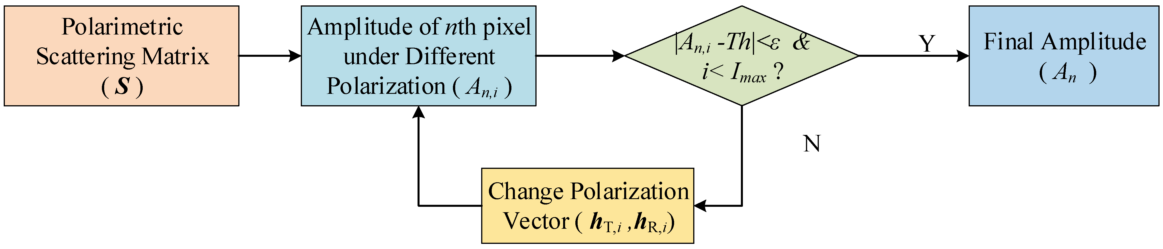
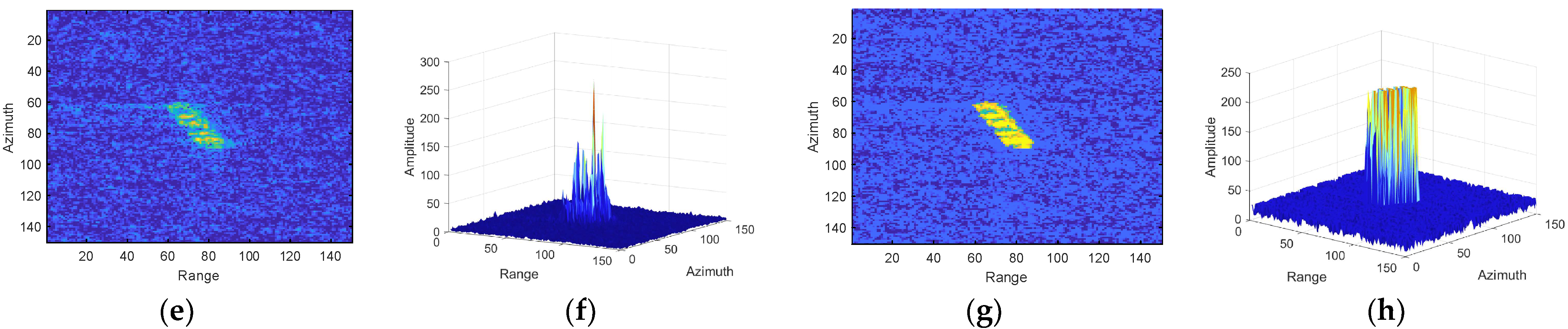
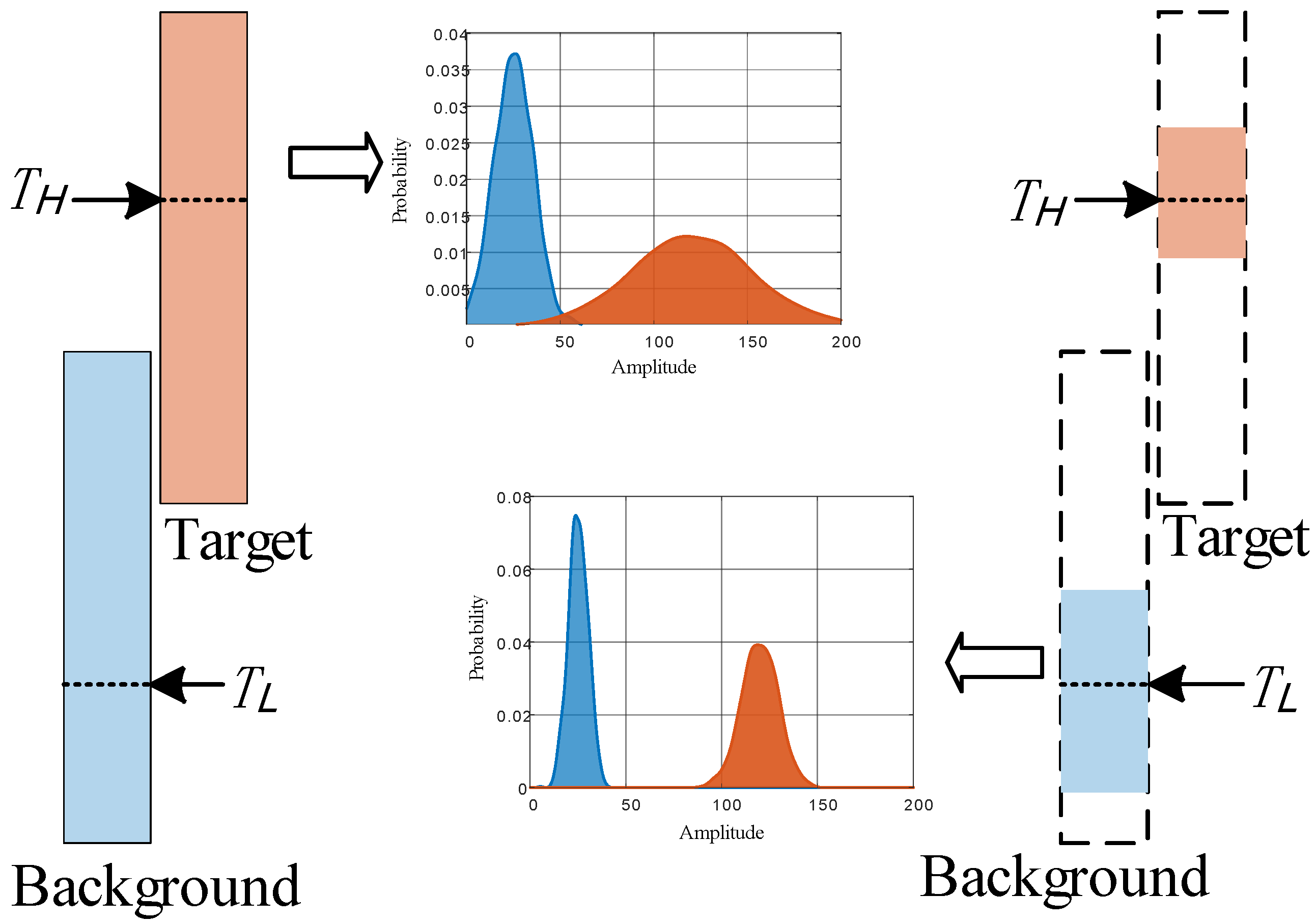
2.3. Amplitude Approximation Strategy Based on Polarization Modulation

To simplify the solution process of the above problem and optimize the effect of polarization modulation, the degree of freedom of polarization modulation is further increased. Considering the PolSAR image processing as a post-processing technique, virtual polarization is employed for polarization modulation. The proposed amplitude approximation strategy theoretically allows for the arbitrary transmitting and receiving of polarization combinations for different pixels. The degree of freedom increases from one or two of the traditional OPCE methods to the number of target pixels $N$.

If the transmitting and receiving polarization combinations are individually optimized for each pixel, the optimal problem of (9) is rewritten as

$$\begin{array}{l}\mathrm{m}\mathrm{i}\mathrm{n} {\displaystyle \sum _{p=1}^{N-1}{\displaystyle \sum _{q=p+1}^N\left|u_{\mathrm{T}p}^{\mathrm{H}}{v}_p-u_{\mathrm{T}q}^{\mathrm{H}}{v}_q\right|}}\\ \mathrm{s}.\mathrm{t}. {\left|v_i\right|}^2=1,i=1,2,\dots N\end{array}$$

(12)

To minimize the objective function, each term is optimized to its lowest possible value. That is to say, the amplitude of samples satisfies $u_{\mathrm{T}1}^{\mathrm{H}}{v}_1=u_{\mathrm{T}2}^{\mathrm{H}}{v}_2=\cdots =u_{\mathrm{T}N}^{\mathrm{H}}{v}_N$.

The polarization response of each pixel in the image at different transmitting and receiving polarizations is $\left|A\right|=\left|u^{\mathrm{H}}v\right|=\left|u\right|\left|v\right|\cos \theta =\left|u\right|\cos \theta$, which takes the range of $\left|A\right|\in \left[0,\left|u\right|\right]$. The maximum value is achieved when the polarization scattering matrix element vector and the transmitting and receiving polarization element vector are in the same direction.

Assuming that the amplitude of each pixel in the image can be modulated by the virtual polarization, they can be modulated to the specified value by setting a suitable threshold $Th$. The threshold can be determined by the target pixels and background pixels, which are chosen according to the pre-segmentation. As illustrated in Figure 2, the amplitude of the $n\mathrm{th}$ pixel under the $i\mathrm{th}$ iteration is $A_{n,i}$. The optimization procedure stops when the error between the target amplitude and the threshold reaches the set minimal value $\epsilon$ or the iteration number reaches the set maximal value $I_{\max }$. It can be inferred that under this procedure, the pixels with the amplitude range after polarization modulation exceeding the threshold can approximate the threshold. However, for pixels with a maximum amplitude below the threshold, it remains significantly distant from the threshold.

With the Gaofen-3 data, we analyzed the image optimization performance of three distinct polarization modulation methods: optimization on the target area as (9), optimization with limited polarization as (11), and the amplitude approximation method. The results are presented in Figure 3 and Figure 4.

The figure presents the HH image of the ship chips and the results derived from various optimization methods. It is evident that when the target region is individually optimized, the amplitude obtained for the target region is relatively low, resulting in a less distinct contrast between the target and the background, as illustrated in Figure 3 and Figure 4c,d. Conversely, with the joint optimization method, while the contrast between the target and background becomes more pronounced, the difference in the target region significantly exceeds that of the original HH channel image, as seen in Figure 3 and Figure 4e,f. However, when employing the amplitude approximation method, there is a more pronounced difference between the target and background regions, and the target region exhibits greater uniformity, as depicted in Figure 3 and Figure 4g,h.

3. Ship Contour Extraction Method from PolSAR Images

This Section introduces a ship segmentation method from polarimetric SAR images, utilizing polarization modulation. The proposed method is divided into three steps: image pre-segmentation, optimization of polarization modulation, and extraction of the ship’s contour. Initially, the image is partitioned into the foreground (target) and background (clutter) using a super-pixel unsupervised clustering approach. Subsequently, based on the preliminary division results, the target amplitude is optimized through the application of polarization modulation. Finally, the ship’s contour is extracted from the optimized image using an edge-detection operator and an adaptive edge extraction algorithm. The flowchart of this algorithm is depicted in Figure 5. The following will provide a detailed description of each part of the algorithm.

3.1. Image Pre-Segmentation Based on Super-Pixel Unsupervised Clustering

Superpixel generation serves as a fundamental image preprocessing technique, playing a pivotal role in various applications including classification, change detection, and target recognition. The superpixel method provides a concise representation of an image by grouping pixels with analogous attributes into locally coherent regions. These localized regions, referred to as superpixels, retain the majority of the information from the grouped pixels. Simple linear iterative clustering (SLIC) [38] is a local clustering-based method. It mainly consists of two stages: initialization of the superpixel centers and local K-mean clustering. To fully utilize the polarization and spatial information, the distance between arbitrary pixel $i$ and pixel $j$ for the clustering is adjusted and represented as $D\left(i,j\right)$.

$$D\left(i,j\right)=\sqrt{{\left({\displaystyle \frac{d_{i,j}^P}{{\tau }_1}}\right)}^2+{\left({\displaystyle \frac{d_{i,j}^S}{{\tau }_2}}\right)}^2}$$

(13)

where $d_{i,j}^P={‖S_i-S_j‖}_2$ denotes the polarization difference and $S_i$,$S_j$ are the scattering matrix of two pixels. $d_{i,j}^S$ denotes the difference between spatial locations $d_{i,j}^S=\sqrt{{\left(x_i-x_j\right)}^2+{\left(y_i-y_j\right)}^2}$. ${\tau }_1$ and ${\tau }_2$ are the quantization factors of the two differences, respectively. Ultimately, the optimal segmentation results are derived iteratively according to the constraints of the iteration numbers and the clustering center movement.

Subsequently, these superpixels are divided into two categories according to the unsupervised clustering and the feature vector is set as

$$F_{\mathrm{SP}}=\left[{\overline{S}}_{\mathrm{HH}},{\overline{S}}_{\mathrm{HV}},{\overline{S}}_{\mathrm{VH}},{\overline{S}}_{\mathrm{VV}}\right]$$

(14)

where ${\overline{S}}_{\mathrm{HH}},{\overline{S}}_{\mathrm{HV}},{\overline{S}}_{\mathrm{VH}},{\overline{S}}_{\mathrm{VV}}$ is the average value of all pixels within the superpixel. Then, the image is partitioned into foreground and background. Figure 6a shows the super-pixel segmentation results of the SLICE algorithm. Then, the super-pixels are divided into two categories. As illustrated in Figure 6b, the foreground marked in red primarily consists of the superpixel where the target is situated, while the background in green comprises the sea surface. Figure 6c shows the amplitude distribution of the foreground and background pixels in Figure 6b. Given that superpixels are inherently over-segmented, the foreground superpixels contain both targets and clutter. It can be discerned from the histograms in Figure 6c, which exhibit some degree of overlap.

3.2. Image Optimization Based on Polarization Modulation

After obtaining the classification result of the target and background through superpixel pre-segmentation, the image is optimized based on the polarization modulation in Section 2. We adopt the strategy of amplitude approximation and propose a dual threshold approximation method for the target and background. The amplitude thresholds of the target and background are $T_H$ and $T_L$, respectively. Then, the following optimization model is constructed to solve for the optimal transmitting and receiving polarization vectors and amplitude thresholds.

$$\begin{array}{l}\mathrm{m}\mathrm{i}\mathrm{n} {\displaystyle \frac{\frac{1}{N}{\displaystyle \sum _{i=1}^N\left|u_{\mathrm{T}i}^{\mathrm{H}}{v}_{\mathrm{T}i}-T_{\mathrm{H}}\right|}+\frac{1}{M}{\displaystyle \sum _{j=1}^M\left|u_{\mathrm{C}j}^{\mathrm{H}}{v}_{\mathrm{C}j}-T_{\mathrm{L}}\right|}}{\left|T_{\mathrm{H}}-T_{\mathrm{L}}\right|}}\\ \mathrm{s}.\mathrm{t}. {\left|v_{\mathrm{T}}\right|}^2=1,{\left|v_{\mathrm{C}}\right|}^2=1 \end{array}$$

(15)

The schematic diagram of the optimization solution and the trend of image amplitude are shown in Figure 7. In the original image, amplitude fluctuations within the target and background result in a broad histogram distribution, with some degree of overlap. However, through dual threshold amplitude approximation optimization, the distribution of the target and background becomes more concentrated. Concurrently, by fine-tuning the thresholds for target and background pixels, the centers of their amplitude distribution are significantly separated.

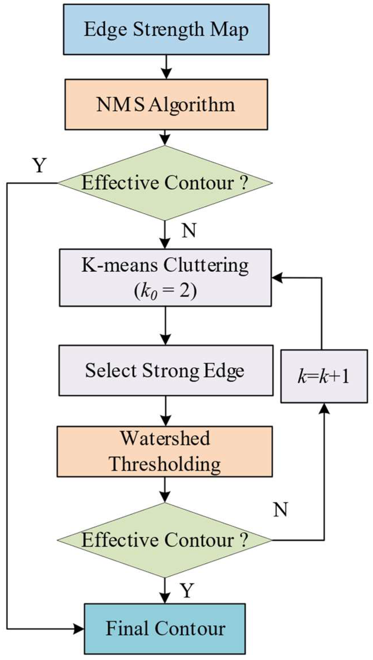
3.3. Edge Extraction Based on ROEWA Detector and Adaptive Clustering

In this Section, edge detection and ship contour extraction will be performed based on optimized images. The ROEWA edge detector is adopted, which is an exponential smoothing filter based on linear least mean square error (LMMSE) proposed by Fjortoft [13]. The expression of the one-dimensional exponential smoothing filter is given by

$$f\left(x\right)=A{e}^{-\alpha \left|x\right|}$$

(16)

where $A$ is the normalized constant and $\alpha$ is the filter coefficient, and (16) can be extended to two dimensions to form $f\left(x,y\right)=f\left(x\right)f\left(y\right)$.

$$f\left(x\right)={\displaystyle \frac{1}{1+b}}{f}_1\left(x\right)+{\displaystyle \frac{b}{1+b}}{f}_2\left(x-1\right),x=1,2,\cdots N$$

(17)

where $f_1\left(x\right)=a\cdot b^x\mathrm{H}\left(x\right)$ is a causal filter and $f_2\left(x\right)=a\cdot b^{-x}\mathrm{H}\left(-x\right)$, $0<b=e^{-\alpha }<1,a=1-b$ is an un-causal filter. $\mathrm{H}\left(x\right)$ is the Heaviside function whose value is 1 if $x\ge 0$, and 0 otherwise. Based on the exponential smoothing filter, the ROEWA operator can be obtained as $r_{\max }={\left[r_{X\max },r_{Y\max }\right]}^{\mathrm{T}}$, where

$$\left\{\begin{array}{l}{r}_{X\max }(x,y)=\max \left\{{\displaystyle \frac{{\widehat{\mu }}_{X1}(x-1,y)}{{\widehat{\mu }}_{X2}(x+1,y)}},{\displaystyle \frac{{\widehat{\mu }}_{X2}(x+1,y)}{{\widehat{\mu }}_{X1}(x-1,y)}}\right\}\hfill \\ r_{Y\max }(x,y)=\max \left\{{\displaystyle \frac{{\widehat{\mu }}_{Y1}(x,y-1)}{{\widehat{\mu }}_{Y2}(x,y+1)}},{\displaystyle \frac{{\widehat{\mu }}_{Y2}(x,y+1)}{{\widehat{\mu }}_{Y1}(x,y-1)}}\right\}\hfill \end{array}\right.$$

(18)

${\widehat{\mu }}_{X1},{\widehat{\mu }}_{X2},{\widehat{\mu }}_{Y1},{\widehat{\mu }}_{Y2}$ are the exponentially weighted average of different directions.

$$\left\{\begin{array}{l}{\widehat{\mu }}_{X1}(x,y)=f_1(x)\ast \left(f(y)\otimes u_0(x,y)\right)\hfill \\ {\widehat{\mu }}_{X2}(x,y)=f_2(x)\ast \left(f(y)\otimes u_0(x,y)\right)\hfill \\ {\widehat{\mu }}_{Y1}(x,y)=f_1(y)\otimes \left(f(x)\ast u_0(x,y)\right)\hfill \\ {\widehat{\mu }}_{Y2}(x,y)=f_2(y)\otimes \left(f(x)\ast u_0(x,y)\right)\hfill \end{array}\right.$$

(19)

where the symbol $\ast$ denote the convolution in the X-direction, the symbol $\otimes$ denote the convolution in the Y-direction, and $u_0(x,y)$ is the current pixel. In summary, the edge strength based on the ROEWA algorithm is obtained as

$$\left|r_{\max }(x,y)\right|=\sqrt{r_{X \max }^2(x,y)+r_{\mathrm{Y} \max }^2(x,y)}$$

(20)

As illustrated in Figure 8, the target edge strength is incomplete and the broken, deformed edges occur when extracting the edge-strength map with the original single-polarization (HH) image. The crippled edge intensity map is not favorable for subsequent contour extraction. However, when utilizing the polarization modulation optimized image for edge-strength extraction, the edges are clearer and more complete, thereby facilitating the ship contour extraction.

After acquiring the edge-strength map, there are two kinds of contour extraction methods: the Watershed thresholding algorithm [15] and the NMS algorithm [16]. The advantage of the watershed algorithm is that the result is a closed boundary, which is convenient for subsequent processing and detection, and can suppress adhesive edges such as line-like non-closed edges. However, the algorithm requires accurate binary segmentation of the gradient, and it is easy to miss the tiny targets. The NMS algorithm yields clear extracted edges with distinct boundaries, eliminating the need for threshold setting. Nevertheless, the contours produced by this algorithm are not closed. To leverage the advantages of both the NMS algorithm and watershed algorithms, this Section introduces a contour extraction algorithm based on adaptive clustering. The proposed adaptive contour extraction algorithm primarily comprises two steps, as depicted in Figure 9.

The NMS method is firstly adopted to find the closed boundary. Nevertheless, in most cases, the NMS algorithm finds it difficult to find the closed boundary. Therefore, the watershed algorithm is subsequently integrated with adaptive clustering to derive the refined contour. The edge-strength map is segmented into two classes according to the k-means algorithm and the class with stronger edge strength is treated as the target edge. The extracted contour is evaluated against two criteria: it must constitute a closed, complete contour and the coverage area of the closed contour makes up a major part of the strong edge region. If these conditions are met, the edge is called the effective contour. Otherwise, further segmentation is conducted with more clustering numbers. To prevent excessive division, a maximum class number limit is set.

As depicted in Figure 10a, there is a discontinuity between the strong edges in the edge-strength map. The contours obtained by NMS have breaks and internal sticking, which leads to a failure to extract closed contours. Moreover, because of the high intensity and unevenness of the background edges, there are more false alarms in the clustering results obtained when the number of clusters is set to two. Meanwhile, there is more interference in the target area, which is not favorable for edge detection. When the number of clustering categories increases to three, the target and background regions are effectively distinguished. By analyzing the edge intensity of each class, the potential region of the target contour is obtained with the largest intensity, as shown in Figure 10e. The watershed algorithm is applied to the strong edges, and the final complete target contour is extracted as shown in Figure 10f.

3.4. Evaluation of Contour Extraction

The MS COCO evaluation metric [39] commonly used for image segmentation, is utilized in this Section. To determine the segmentation accuracy of individual targets, the intersection and union ratio (IoU) is evaluated. Then, the segmentation accuracy of the entire dataset is evaluated using the F1-score metric. Firstly, by comparing the ground truth label and the detected contour, the ratio of the concatenation and intersection area of the two is calculated to measure the fineness of image segmentation.

$$IoU={\displaystyle \frac{G\cap D}{G\cup D}}$$

(21)

where $G$ and $D$ denote the ground truth and contour extraction result, respectively.

If the IoU ratio exceeds a predetermined threshold (typically 0.5), the target is deemed correctly detected (TP). Conversely, if the detected contour fails to align with the actual contour, it is classified as a false positive (FP). If there is no corresponding correct detection for the actual contour, it is categorized as a missed detection (FN). Subsequently, accuracy and recall are computed using the following formulas

$$Precision={\displaystyle \frac{TP}{TP+FP}}$$

(22)

$$Recall={\displaystyle \frac{TP}{TP+FN}}$$

(23)

Then, the F1 scores of the entire dataset are calculated as

$$F_1=2{\displaystyle \frac{Precision\cdot Recall}{Precision+Recall}}$$

(24)

3.5. Extraction of Geometric Features

The purpose of ship segmentation and contour extraction is to obtain the geometric shape and size, thereby enhancing the accuracy of target recognition. There are primarily two methods for extracting ship geometric features. The first method involves directly obtaining the size of the target based on the image and the extracted ship contour, which includes techniques such as the Hough transform, rectangular fitting, and ellipse fitting method. The second method employs a multivariate linear model that describes the actual size of the ship as a function of target information (such as length, width, angle of ship mask in images), observation information (such as observation angle), and other relevant parameters. The relationship between these variables is determined by optimization [5,40,41]. Since the second method integrates multiple factors, it may not be suitable for evaluating the performance of target contour extraction. Therefore, we primarily focus on the first method.

Since the contour shape of the ship in the SAR image is mainly elliptical, after obtaining the coordinates of the contour points, Fitzgibbon’s ellipse fitting method [42] is used to fit these points to obtain the corresponding ellipse parameters. A conic curve in the $x-y$ plane can be expressed by a quadratic polynomial.

$$F(a;x)=a^{\mathrm{T}}x=a{x}^2+bxy+c{y}^2+dx+ey+f=0$$

(25)

where $a={\{a,b,c,d,e,f\}}^{\mathrm{T}},x={\left\{x^2,xy,y^2,x,y,1\right\}}^{\mathrm{T}}$.$F(a;x_i)$ denotes the distance from a point with coordinates $x_i=\left(x_i,y_i\right)$ to the curve, and the curve is fitted by minimizing the square sum of the distances among these $N$ points.

$$E(a)={\displaystyle \sum _{i=0}^{n}F{(a;x_i)}^2}$$

(26)

Under the constraints of the equation $4ac-b^2=1$, the curve represents an elliptic curve. The elliptic fitting problem can be expressed as

$$\begin{array}{l}\mathrm{m}\mathrm{i}\mathrm{n}\mathrm{||}{J}^{\mathrm{T}}Ja{\mathrm{||}}^2\\ \mathrm{s}.\mathrm{t}. a^{\mathrm{T}}Ca=1\end{array}$$

(27)

where $J={\left\{x_1,x_2,\dots ,x_n\right\}}^{\mathrm{T}}$. $C$ is the transformation matrix of the equation constraints. The above optimization problem of equality constraint can be solved with the Lagrange multiplier method. The result of ellipse fitting is shown in Figure 11a, where the green curve represents the detected ship contour, and the red curve is the result of target ellipse fitting. According to the ellipse equation, the major axis $A$, the minor axis $B$, and the orientation angle $\theta$ of the ellipse can be calculated, where the ellipse orientation is the angle between the major axis of the ellipse and the vertical line. Due to the fact that the front and back of ships cannot be discriminated, the orientation angle $\theta$ is manually corrected to the range of 0° and 90°. The parameters of the ellipse are shown in Figure 11b.

On this basis, the length $L$, width $W$, and orientation angle ${\theta }_s$ of the ship are calculated based on the imaging geometric relationship and imaging resolution. Assuming that the imaging resolution in azimuth and range are ${\delta }_{\mathrm{A}},{\delta }_{\mathrm{R}}$, the geometric parameters of the target can be calculated as

$$L=\sqrt{{\left(A\cdot {\delta }_{\mathrm{A}}\sin \theta \right)}^2+{\left(B\cdot {\delta }_{\mathrm{R}}\cos \theta \right)}^2},W=\sqrt{{\left(A\cdot {\delta }_{\mathrm{A}}\cos \theta \right)}^2+{\left(B\cdot {\delta }_{\mathrm{R}}\sin \theta \right)}^2},{\theta }_{\mathrm{S}}={\theta }_N-\theta$$

(28)

where ${\theta }_N$ is the angle between the range direction in the imaging geometry and the north direction.

Two criteria are used to check the performance of the geometric features including the absolute and relative errors. The estimation errors are obtained by comparing them with the corresponding AIS information. Two types of errors are derived: average absolute error (AE), and average relative error (RE).

$$AE=\left|A_{\mathrm{Estimated}}-A_{\mathrm{True}}\right|,RE={\displaystyle \frac{AE}{A_{\mathrm{True}}}}$$

(29)

where $A_{\mathrm{Estimated}}$ and $A_{\mathrm{True}}$ are the estimated and true values, respectively.

4. Experimental Results and Performance Analysis

4.1. Dataset

Gaofen-3 satellite is China’s first civil C-band high-resolution quad-pol SAR satellite specifically missioned for ocean remote sensing. The nominal highest resolution of Gaofen-3 data is up to 1 m. Gaofen-3 data have been widely used in applications such as ship recognition, environmental monitoring, urban planning, and disaster management [43]. In this Section, we construct the ship contour extraction dataset with Gaofen-3 PolSAR images collected near the Hong Kong area. The three PolSAR images encompass a variety of ships, including both near-shore and far-shore vessels. Based on the image and AIS information [44], combined with the expert knowledge, the ground truth of the ship contour is labeled. A total of 139 labeled ship chips are obtained, and the size of the chips is 150 × 150. The fundamental details of the data and the labeling results are presented in

Table 1. Data information of selected PolSAR images.

No.	Resolution (Range × Azimuth)	Image Size (Range × Azimuth)	Incidence Angle	Number of Ships
1	4.49 m × 4.99 m	4086 × 5733	48.72°	59
2	4.49 m × 4.99 m	4086 × 5733	48.72°	6
3	2.25 m × 4.76 m	7297 × 6822	32.03°	74

and Figure 12, respectively. The area delineated by the red box in the optical image corresponds to the data acquisition region. The SAR image is labeled with the ship’s contour and number. To illustrate the labeling results of the ship chips, a single ship is chosen from each view of the PolSAR image for closer examination. It is evident that the green ship outline aligns closely with the target area of the ship depicted in the image.

4.2. Performance Analysis of Contour Extraction

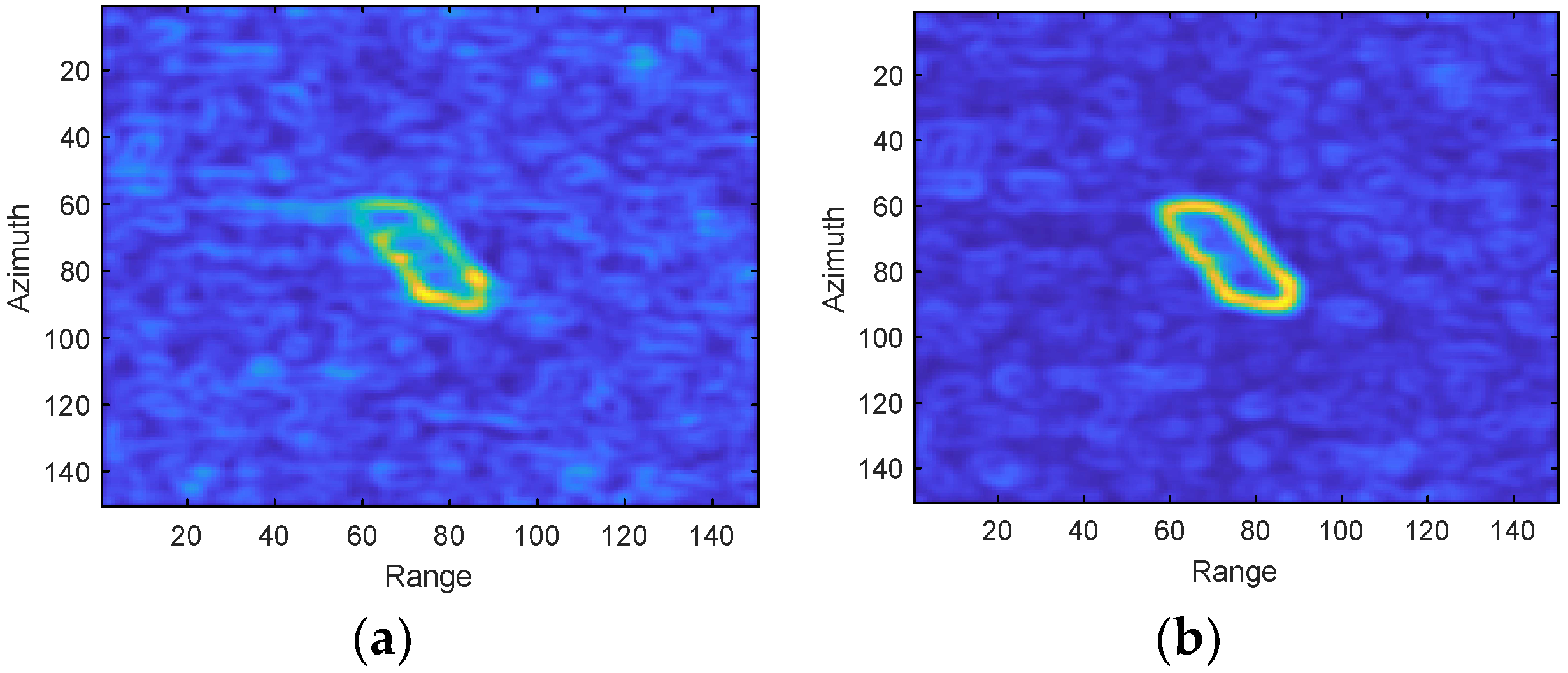
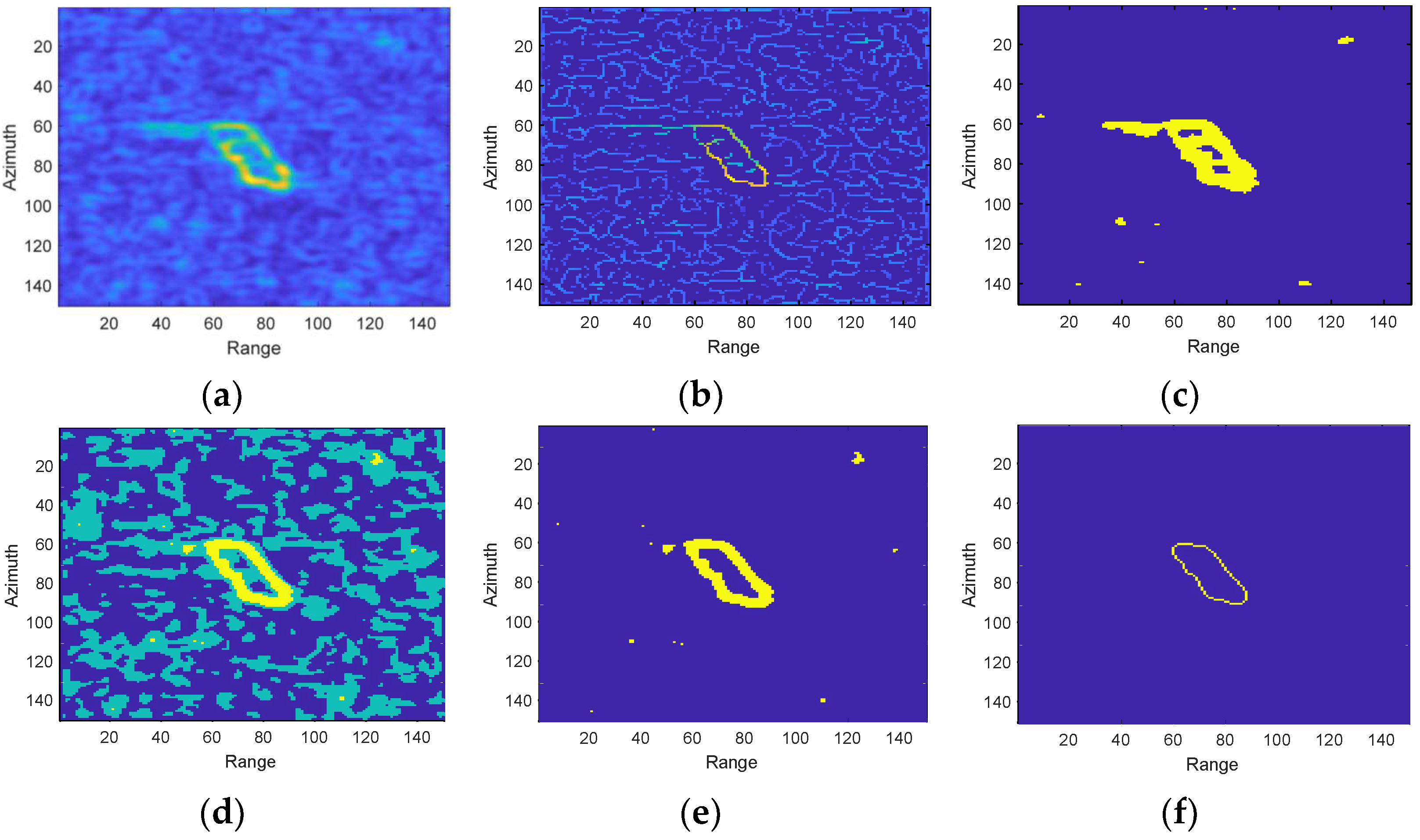
4.2.1. Contour Extraction of Specific Scenes

This Section considers the following two scenarios, which are zoomed-in images of data No. 1 in Table 1. One is a single-target scenario where there are strong scattering centers within the target and the internal amplitude distribution is not uniform. The second is a multi-target scenario, where there are multiple targets within the same scene and there are differences in target amplitudes. Ship contour extraction analysis is performed on single-polarization images and images after polarization modulation, respectively. The contour extraction method is the ROEWA edge detector with the adaptive clustering algorithm, as illustrated in Section 3.

• Single-target scene

The PolSAR images of a single target, along with the results of contour extraction, are depicted in Figure 13. For the three single-polarization images, there are noticeable strong scattering centers, and the amplitude within the target is not consistent. The ROEWA edge detector is employed to extract the edge strength. It can be observed that there are distinct edges around strong scatters of the single-polarization image, resulting in a weak external edge intensity. Meanwhile, the internal edge strength of the target is uneven, which consequently results in over-segmentation of the target. Furthermore, a comparison of the edge-strength results across various polarization channels reveals the complementarity within the full polarization data. The strong edges of the target across the three polarization channels manifest at distinct locations. With polarization modulation, the amplitude of the target’s internal pixel tends to be uniform. Consequently, in the extracted edge intensity image, the target edge has a uniform and large intensity, which can clearly indicate the target contour. A comprehensive and precise target contour can be obtained through the contour extraction algorithm.

b.

Multi-target scene

As illustrated in Figure 14, the amplitude of various targets differs within the single-polarization images. The presence of strong targets often renders weaker ones as background noise. In the edge intensity map extracted from these single-polarization images, the edges of weaker targets are isolated points, thus failing to form effective contours. Therefore, the probability of missing detection is significantly high. However, when utilizing a polarization modulation-optimized image, the internal amplitudes of all targets are uniform, and the contour can be accurately extracted.

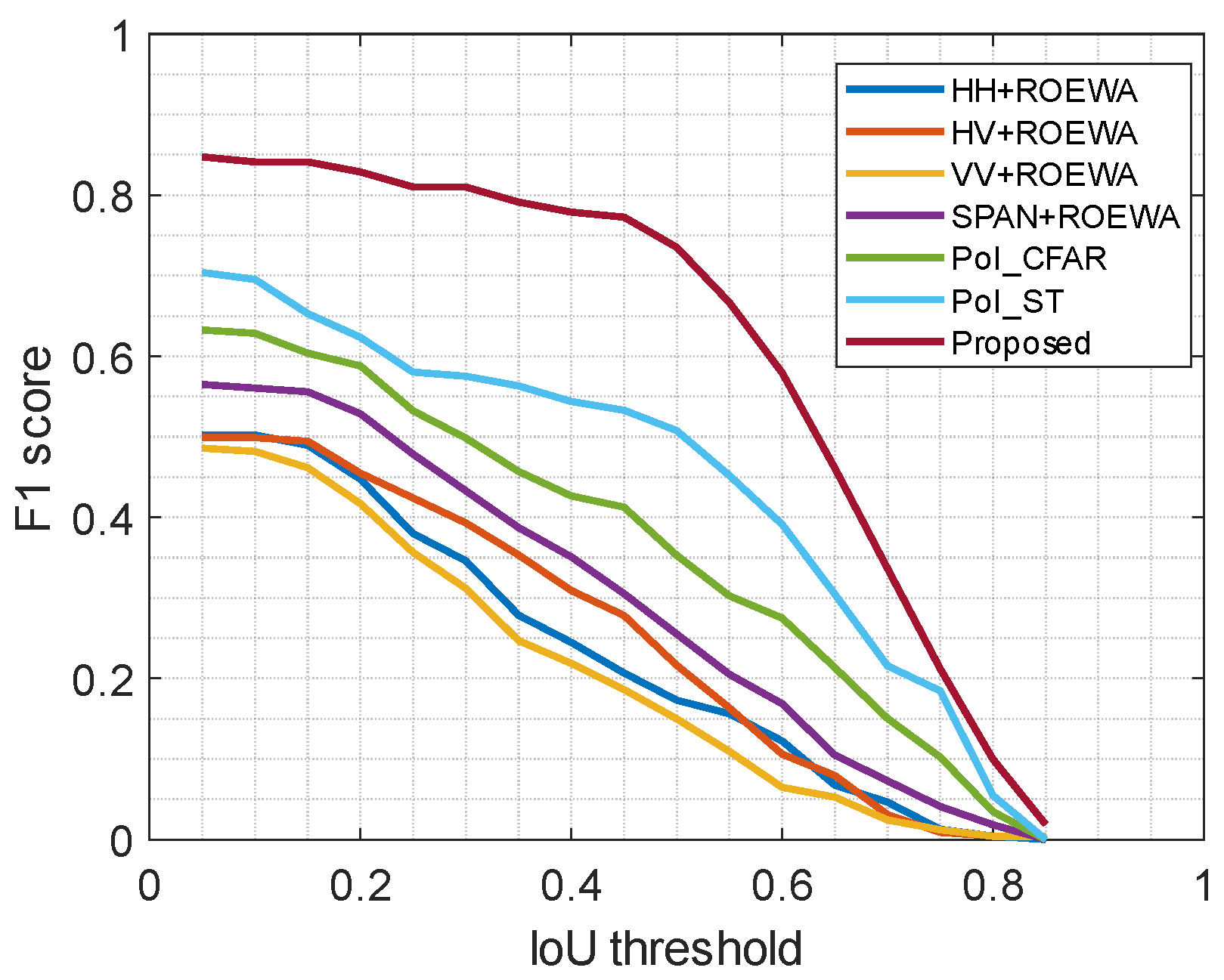
4.2.2. Contour Extraction Accuracy of the Whole Dataset

To present the superior performance of the polarization modulation optimization, the proposed method is compared with the same ROEWA edge detector performed on the single-polarization images (HH, HV, VV) and the fusion of four images (SPAN). Moreover, several state-of-the-art PolSAR image edge detectors are compared, including the CFAR edge detector with the SIRV Model for PolSAR images (Pol-CFAR) [30] and the structure tensor operator for PolSAR images (Pol-ST) [31]. It is worth noting that the edge-strength maps of all methods deal with the same post-processing, as illustrated in Figure 9.

By setting different IoU thresholds, the detection performance of different methods can be obtained, as illustrated in Figure 15. The results indicate that the cross-polarized channels have the best performance among the single-polarization images. Furthermore, the performance of the total power obtained by the fusion of polarization channels is better than that of single-polarization channels, but the enhancement is not significant. In terms of the optimized image after polarization modulation, there is a significant improvement in the F1-scores of the detection results, outperforming other methods.

4.2.3. Comparison of Computational Complexity

The proposed method, which employs an amplitude optimization technique for edge detection, is compared with methods based on the ROEWA operator for SAR images, Pol-CFAR, and Pol-ST. The experiments are implemented on a desktop with an Intel Core i7-9750H central processing unit with a frequency of 2.6 GHz and 32 GB random access memory. The algorithm is programmed using MATLAB language.

Table 2. Execution time comparison of the different methods (in seconds).

	Single-Target Scene (250 × 300)	Multi Target Scene (400 × 500)
ROEWA	4.90	12.72
Pol-CFAR	12.51	35.12
Pol-ST	10.11	28.54
Proposed	15.01	40.08

gives the execution time of the different methods. It can be seen that the time costs of Pol-CFAR and Pol-ST are comparable, whereas the proposed method takes a longer time than the others. Considering that the time cost of the ROEWA operator is notably low, the main time cost of the proposed method comes from the superpixel segmentation and amplitude optimization.

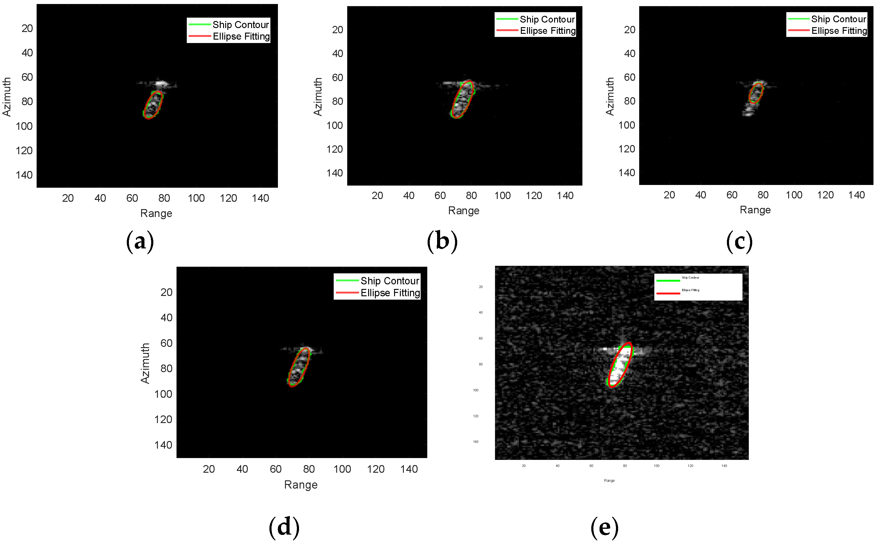
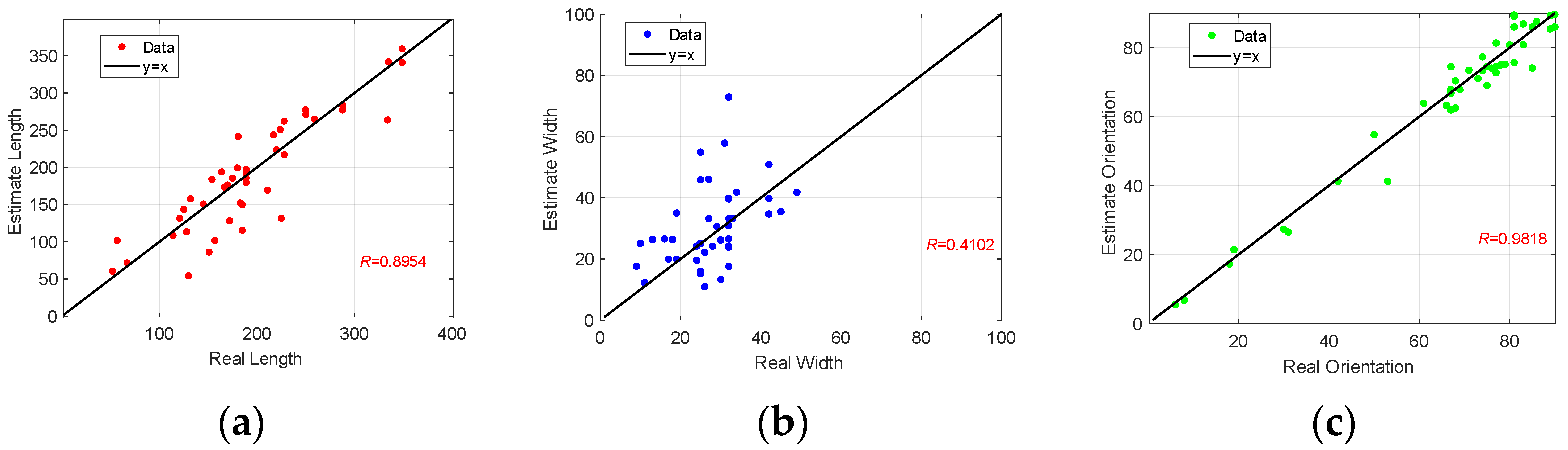
4.2.4. Performance Analysis of Geometric Features Extraction

To measure the effectiveness of ship contour extraction, we extract the geometric parameters of the target and evaluate the estimation errors in combination with the AIS information. The results of ship contour extraction and ellipse fitting for images with different polarization channels and polarization modulation are shown in Figure 16. In the single-polarization channel, the incomplete ship contour leads to a serious deviation of the fitted ellipse from the target region. The results of HV and SPAN are better than those of HH and VV. However, the ellipse boundaries extracted from the results of the two images have some degree of shrinkage, and the estimated length will be smaller than the true value. In contrast, the polarization modulation method combines information from various polarization channels and obtains more complete fitting results.

Based on the extracted ship contour, the dimensional information such as the length and width of the target is derived by the method introduced in Section 3. The results of ship geometry feature extraction are shown in Figure 17. The horizontal axis is the real size information of the ship, and the vertical axis is the estimation result. The $R$ is the correlation coefficient between them. The estimation errors are listed in

Table 3. Error analysis of geometric feature extraction.

	Average Length Error (AE/RE)	Average Width Error (AE/RE)	Average Orientation Error (AE)
HH	53.09 m/28.42%	11.31 m/45.56%	5.13°
HV	28.51 m/15.52%	9.68 m/39.76%	3.62°
VV	51.40 m/27.53%	11.64 m/46.76%	5.04°
SPAN	22.61 m/12.42%	9.32 m/38.46%	3.36°
Proposed	20.09 m/11.10%	8.96 m/37.17%	3.02°

. The analysis reveals that the estimated orientation of ships in the polarization modulation images exhibits the highest accuracy, with a correlation between the actual and estimated orientation reaching an impressive 0.9818. The length estimation accuracy follows closely, presenting an average absolute error of 20.09 m. Conversely, the width extraction accuracy is the least satisfactory, displaying a relative error as high as 37.17%, despite an average absolute error of approximately 9 m. This discrepancy can be attributed to factors such as image resolution and the precision of the ship’s AIS information. Furthermore, a comparison of the size estimation errors between the single-polarization image and the SPAN image reveals that the method proposed in this paper exhibits superior extraction accuracy.

5. Conclusions

The amplitude variation of a target within a single-polarization SAR image often results in over-segmentation and the missed detection of weak targets when using traditional edge-detection algorithms. To solve this problem, we leverage the polarization’s ability to modulate target amplitude and make attempts to extract the ship contour from PolSAR images. A comprehensive framework is developed for extracting ship contours in PolSAR images. We propose an optimization method for polarization modulation under the uniform criterion of target amplitude. The degrees of freedom for polarization modulation are increased and the approximate solution of the optimization model is achieved by threshold approximation. In addition, in order to improve the optimization efficiency and the accuracy of edge extraction, a foreground–background division method with superpixel preprocessing and an edge extraction method with adaptive clustering are proposed.

In this work, a ship segmentation PolSAR dataset is constructed with Gaofen-3 PolSAR images, combined with expert knowledge and AIS information. The experimental results indicate that the accuracy of ship contour extraction with the proposed method markedly surpasses that of single PolSAR images and other state-of-the-art methods. Furthermore, the extracted geometric features exhibit high precision. For targets with specific geometrical shapes, such as linear and circular, it is necessary to design corresponding constraints and judgment criteria, which will be researched in our future work.

References

1. Cumming, I.G.; Wong, F.H. Digital Processing of Synthetic Aperture Radar Data: Algorithms and Implementation; Artech House: London, UK, 2005. [Google Scholar]
2. Yasir, M.; Liu, S.; Pirasteh, S.; Xu, M.; Sheng, H.; Wan, J.; de Figueiredo, F.A.P.; Aguilar, F.J.; Li, J. YOLOShipTracker: Tracking Ships in SAR Images Using Lightweight YOLOv8. Int. J. Appl. Earth Obs. Geoinf. 2024, 134, 104137. [Google Scholar] [CrossRef]
3. Touzi, R.; Lopes, A.; Bousquet, P. A statistical and geometrical edge detector for SAR images. IEEE Trans. Geosci. Remote Sens. 1988, 26, 764–773. [Google Scholar] [CrossRef]
4. Gemme, L.; Dellepiane, S.G. An automatic data-driven method for SAR image segmentation in sea surface analysis. IEEE Trans. Geosci. Remote Sens. 2018, 56, 2633–2646. [Google Scholar] [CrossRef]
5. Li, B.; Liu, B.; Guo, W.; Zhang, Z.; Yu, W. Ship size extraction for sentinel-1 images based on dual-polarization fusion and nonlinear regression: Push error under one pixel. IEEE Trans. Geosci. Remote Sens. 2018, 56, 4887–4905. [Google Scholar] [CrossRef]
6. Xiang, D.; Tang, T.; Quan, S.; Guan, D.; Su, Y. Adaptive superpixel generation for SAR images with linear feature clustering and edge constraint. IEEE Trans. Geosci. Remote Sens. 2019, 57, 3873–3889. [Google Scholar] [CrossRef]
7. Wei, S.; Zeng, X.; Zhang, H.; Zhou, Z.; Shi, J.; Zhang, X. LFG-Net: Low-level feature guided network for precise ship instance segmentation in SAR images. IEEE Trans. Geosci. Remote Sens. 2022, 60, 1–17. [Google Scholar] [CrossRef]
8. Wang, X.; Li, G.; Plaza, A.; He, Y. Revisiting SLIC: Fast superpixel segmentation of marine SAR images using density features. IEEE Trans. Geosci. Remote Sens. 2022, 60, 1–18. [Google Scholar] [CrossRef]
9. Zhao, M.; Zhang, X.; Kaup, A. Multitask learning for SAR ship detection with gaussian-mask joint segmentation. IEEE Trans. Geosci. Remote Sens. 2023, 61, 1–16. [Google Scholar] [CrossRef]
10. Song, S.; Dai, Y.; Sun, S.; Jin, T. Efficient Image Reconstruction Methods Based on Structured Sparsity for Short-Range Radar. IEEE Trans. Geosci. Remote Sens. 2024, 62, 1–15. [Google Scholar] [CrossRef]
11. Pitas, I. Digital Image Processing Algorithms and Applications; John Wiley & Sons: Hoboken, NJ, USA, 2000. [Google Scholar]
12. Ganugapati, S.; Moloney, C. A ratio edge detector for speckled images based on maximum strength edge pruning. In Proceedings of the International Conference on Image Processing, Washington, DC, USA, 23–26 October 1995. [Google Scholar]
13. Fjortoft, R.; Lopes, A.; Marthon, P.; Cubero-Castan, E. An optimal multiedge detector for SAR image segmentation. IEEE Trans. Geosci. Remote Sens. 1998, 36, 793–802. [Google Scholar] [CrossRef]
14. Ostu, N. A threshold selection method from gray-level histograms. IEEE Trans. Syst. Man Cybern. 1979, 9, 62–66. [Google Scholar]
15. Vincent, L.; Soille, P. Watersheds in digital spaces: An efficient algorithm based on immersion simulations. IEEE Trans. Pattern Anal. Mach. Intell. 1991, 13, 583–598. [Google Scholar] [CrossRef]
16. Rosenfeld, A.; Thurston, M. Edge and Curve Detection for Visual Scene Analysis. IEEE Trans. Comput. 1971, C-20, 562–569. [Google Scholar]
17. Trier, O.D.; Jain, A.K. Goal-directed evaluation of binarization methods. IEEE Trans. Pattern Anal. Mach. Intell. 1995, 17, 1191–1201. [Google Scholar] [CrossRef]
18. Bernsen, J. Dynamic thresholding of gray-level images. In Proceedings of the International Conference on Pattern Recognition, Paris, France, 27–31 October 1986; pp. 1251–1255. [Google Scholar]
19. Kass, M.; Witkin, A.; Terzopoulos, D. Snakes: Active contour models. Int. J. Comput. Vis. 1988, 1, 321–331. [Google Scholar] [CrossRef]
20. Cohen, L.D. On active contour models and balloons. CVGIP Image Underst. 1991, 53, 211–218. [Google Scholar] [CrossRef]
21. Xu, C.; Prince, J.L. Snakes, shapes, and gradient vector flow. IEEE Trans. Image Process. 1998, 7, 359–369. [Google Scholar]
22. Osher, S.; Sethian, J.A. Fronts propagating with curvature dependent speed: Algorithms based on Hamilton Jacobi formulations. J. Comput. Phys. 1988, 79, 12–49. [Google Scholar] [CrossRef]
23. Caselles, V.; Catt’e, F.; Coll, T.; Dibos, F. A geometric model for active contours in image processing. Numer. Math. 1993, 66, 1–31. [Google Scholar] [CrossRef]
24. Malladi, R.; Sethian, J.A.; Vemuri, B.C. Shape modeling with front propagation: A level set approach. IEEE Trans. Pattern Anal. Mach. Intell. 1995, 17, 158–175. [Google Scholar] [CrossRef]
25. Gao, F.; Han, X.; Wang, J.; Sun, J.; Hussain, A.; Zhou, H. SAR ship instance segmentation with dynamic key points information enhancement. IEEE J. Sel. Top. Appl. Earth Obs. Remote Sens. 2024, 17, 11365–11385. [Google Scholar] [CrossRef]
26. Gao, F.; Zhong, F.; Sun, J.; Hussain, A.; Zhou, H. BBox-Free SAR hip instance segmentation method based on gaussian heatmap. IEEE Trans. Geosci. Remote Sens. 2024, 62, 1–18. [Google Scholar]
27. Jiang, M.; Gu, L.; Li, X.; Gao, F.; Jiang, T. Ship contour extraction rom SAR images based on faster R-CNN and Chan-Vese model. IEEE Trans. Geosci. Remote Sens. 2023, 61, 1–14. [Google Scholar]
28. Zhang, T.; Zhang, X.; Li, J.; Xu, X.; Wang, B.; Zhan, X.; Xu, Y.; Ke, X.; Zeng, T.; Su, H.; et al. SAR ship detection dataset (SSDD): Official release and comprehensive data analysis. Remote Sens. 2021, 13, 3690. [Google Scholar] [CrossRef]
29. Schou, J.; Skriver, H.; Nielsen, A.A.; Conradsen, K. CFAR Edge Detector for Polarimetric SAR Images. IEEE Trans. Geosci. Remote Sens. 2003, 41, 20–32. [Google Scholar] [CrossRef]
30. Xiang, D.; Ban, Y.; Wang, W.; Tang, T.; Su, Y. Edge Detector for Polarimetric SAR Images Using SIRV Model and Gauss-Shaped Filter. IEEE Geosci. Remote Sens. Lett. 2016, 13, 1661–1665. [Google Scholar] [CrossRef]
31. Gomez, L.; Alvarez, L.; Frery, A.C. Local Edginess Measures in PolSAR Imagery by Using Stochastic Distances. In Proceedings of the IGARSS 2018—2018 IEEE International Geoscience and Remote Sensing Symposium, Valencia, Spain, 22–27 July 2018; pp. 5796–5799. [Google Scholar]
32. Zhuang, Z.; Xiao, S.; Wang, X. Radar Polarization Information Processing and Application; National Defense Industry Press: Arlington, VA, USA, 1999. [Google Scholar]
33. Xie, N.; Zhang, T.; Guo, W.; Zhang, Z.; Yu, W. Dual branch deep network for ship classification of dual-polarized SAR images. IEEE Trans. Geosci. Remote Sens. 2024, 62, 5207415. [Google Scholar] [CrossRef]
34. Xiang, D.; Ding, H.; Sun, X.; Cheng, J.; Hu, C.; Su, Y. PolSAR image registration combining Siamese multiscale attention network and joint filter. IEEE Trans. Geosci. Remote Sens. 2024, 62, 5208414. [Google Scholar] [CrossRef]
35. Wang, S.L.; Wang, X.S.; Xu, Z.H. Principle and approach to polarization modulation for radar super-resolution. Sci. Sin. Informationis 2023, 148, 993–1008. [Google Scholar] [CrossRef]
36. Deng, Q.; Chen, J.; Yang, J. Optimization of polarimetric contrast enhancement based on Fisher criterion. IEICE Trans. Commun. 2009, 92, 3968–3971. [Google Scholar] [CrossRef]
37. Yang, J.; Yamaguchi, Y.; Boerner, W.-M.; Lin, S. Numerical methods for solving the optimal problem of contrast enhancement. IEEE Trans. Geosci. Remote Sens. 2000, 38, 965–971. [Google Scholar] [CrossRef]
38. Achanta, R.; Shaji, A.; Smith, K.; Lucchi, A.; Fua, P.; Süsstrunk, S. Slic superpixels compared to state-of-the-art superpixel methods. IEEE Trans. Pattern Anal. Mach. Intell. 2012, 34, 2274–2282. [Google Scholar] [CrossRef] [PubMed]
39. Lin, T.Y.; Maire, M.; Belongie, S.; Hays, J.; Perona, P.; Ramanan, D.; Doll, P.; Zitnick, C.L. Microsoft coco: Common objects in context. In Proceedings of the Computer Vision—ECCV 2014: 13th European Conference, Zurich, Switzerland, 6–12 September 2014; Proceedings, Part V 13. Springer: Berlin/Heidelberg, Germany, 2014; pp. 740–755. [Google Scholar]
40. Tings, B.; Bentes da Silva, C.A.; Lehner, S. Dynamically adapted ship parameter estimation using TerraSAR-X images. Int. J. Remote Sens. 2016, 37, 1990–2015. [Google Scholar] [CrossRef]
41. Yasir, M.; Liu, S.; Mingming, X.; Wan, J.; Pirasteh, S.; Dang, K.B. ShipGeoNet: SAR image-based geometric feature extraction of ships using convolutional neural networks. IEEE Trans. Geosci. Remote Sens. 2024, 62, 5202613. [Google Scholar] [CrossRef]
42. Fitzgibbon, A.; Pilu, M.; Fisher, R.B. Direct least square fitting of ellipses. IEEE Trans. Pattern Anal. Mach. Intell. 1999, 21, 476–480. [Google Scholar] [CrossRef]
43. Zhao, L.; Zhang, Q.; Li, Y.; Qi, Y.; Yuan, X.; Liu, J.; Li, H. China’s Gaofen-3 Satellite System and Its Application and Prospect. IEEE J. Sel. Top. Appl. Earth Obs. Remote Sens. 2021, 148, 11019–11028. [Google Scholar] [CrossRef]
44. Hou, X.; Ao, W.; Song, Q.; Lai, J.; Wang, H.; Xu, F. FUSAR-Ship: Building a High-Resolution SAR-AIS Matchup Dataset of Gaofen-3 for Ship Detection and Recognition. Sci. China Inf. Sci. 2020, 63, 1–19. [Google Scholar] [CrossRef]
Figure 1. The ship segmentation result of the SSDD dataset: (a) Ground truth of PSeg No. 421. (b) Segmentation result. (c) Ground-truth of PSeg No. 328. (d) Segmentation result.
Remotesensing 16 03669 g001
Figure 2. The procedure of amplitude approximation method.
Remotesensing 16 03669 g002
Figure 3. The Gaofen-3 ship chips and polarization modulation results for a single target: (a) 2D image of HH. (b) 3D image of HH. (c) 2D image of optimization on the target area. (d) 3D image of optimization on the target area. (e) 2D image of joint optimization. (f) 3D image of joint optimization. (g) 2D image of amplitude approximation. (h) 3D image of amplitude approximation.
Remotesensing 16 03669 g003aRemotesensing 16 03669 g003b
Figure 4. The Gaofen-3 ship chips and polarization modulation results for multiple targets: (a) 2D image of HH. (b) 3D image of HH. (c) 2D image of optimization on the target area. (d) 3D image of optimization on the target area. (e) 2D image of joint optimization. (f) 3D image of joint optimization. (g) 2D image of amplitude approximation. (h) 3D image of amplitude approximation.
Remotesensing 16 03669 g004
Figure 5. The procedure of contour extraction algorithm of PolSAR images.
Remotesensing 16 03669 g005
Figure 6. Superpixel segmentation results and Superpixel-based foreground–background classification results: (a) Superpixel segmentation results; (b) Superpixel-based foreground–background classification results; (c) Amplitude distribution of foreground and background superpixels.
Remotesensing 16 03669 g006
Figure 7. Schematic diagram of dual threshold polarization modulation.
Remotesensing 16 03669 g007
Figure 8. Edge strength extracted by ROEWA operator before and after image enhancement: (a) Edge strength of original image (HH); (b) Edge strength of optimized image.
Remotesensing 16 03669 g008
Figure 9. Flowchart of adaptive contour extraction method.
Remotesensing 16 03669 g009
Figure 10. Contour extraction method of adaptive clustering: (a) Edge strength of original image; (b) NMS result; (c) Cluttering result (k = 2); (d) Cluttering result (k = 3); (e) Strong edge; (f) Final contour.
Remotesensing 16 03669 g010
Figure 11. The result of ellipse fitting and schematic of ellipse parameters: (a) The ellipse fitting result; (b) The parameters of ellipse.
Remotesensing 16 03669 g011
Figure 12. The optical images of the selected dataset and the PolSAR images with labels: (a) The optical image of data No. 1; (b) The optical image of data No. 2; (c) The optical image of data No. 3; (d) The labeled image of data No. 1; (e) The labeled image of data No. 2; (f) The labeled image of data No. 3.
Remotesensing 16 03669 g012
Figure 13. Contour extraction results of single-target PolSAR images: (ad) are the intensity of HH, HV, VV, and polarization modulation image, respectively. (eh) are the edge-strength map of HH, HV, VV, and polarization modulation, respectively. (il) are the contour results of HH, HV, VV, and polarization modulation, respectively.
Remotesensing 16 03669 g013
Figure 14. Contour extraction results of multi-target PolSAR images: (ad) are the intensity of HH, HV, VV, and polarization modulation image, respectively. (eh) are the edge-strength map of HH, HV, VV, and polarization modulation, respectively. (il) are the contour results of HH, HV, VV, and polarization modulation, respectively.
Remotesensing 16 03669 g014
Figure 15. Detection results at different IoU thresholds.
Remotesensing 16 03669 g015
Figure 16. The results of ship contour and ellipse fitting with different images: (ae) are the fitting results of HH, HV, VV, SPAN, and polarization modulation images, respectively.
Remotesensing 16 03669 g016
Figure 17. Ship size extraction results: (ac) are the extraction results of length, width, and orientation, respectively.
Remotesensing 16 03669 g017