Enhancing Accuracy in Historical Forest Vegetation Mapping in Yunnan with Phenological Features, and Climatic and Elevation Variables

Abstract

Human activities have both positive and negative impacts on forests, altering the extent and composition of various forest vegetation types, and increasing uncertainty in ecological management. A detailed understanding of the historical distribution of forest vegetation is crucial for local conservation efforts. In this study, we integrated phenological features with climatic and terrain variables to enhance the mapping accuracy of forest vegetation in Yunnan. We mapped the historical distributions of five forest vegetation type groups and nine specific forest vegetation types for 2001, 2010, and 2020. Our findings revealed that: (1) rubber plantations can be effectively distinguished from other forest vegetation using phenological features, coniferous forests and broad-leaved forests can be differentiated using visible spectral bands, and environmental variables (temperature, precipitation, and elevation) are effective in differentiating forest vegetation types under varying climate conditions; (2) the overall accuracy and kappa coefficient increased by 14.845% and 20.432%, respectively, when climatic variables were combined with phenological features, and by 13.613% and 18.902%, respectively, when elevation was combined with phenological features, compared to using phenological features alone; (3) forest cover in Yunnan increased by 2.069 × 10⁴ km² (10.369%) between 2001 and 2020. This study highlights the critical role of environmental variables in improving the mapping accuracy of forest vegetation in mountainous regions.

1. Introduction

Forests cover approximately one-third of terrestrial areas [1] and dominate various ecosystem services, including climate regulation, soil conservation, and the provision of biological habitats [2,3]. The distribution of forest vegetation is influenced by both natural and anthropogenic factors, such as land use changes and climate shifts [4,5,6]. Previous studies have demonstrated that the ecosystem services and biodiversity provided by secondary forests, which result from human activities, are often inferior to those of natural forests [7,8,9]. Consequently, a thorough understanding of the historical distribution of various forest vegetation types is crucial. This knowledge can help elucidate the driving forces behind human impacts on forestry and ecosystem services, informing policymakers in the development of strategies for the protection, restoration, and sustainable management of forests.

Earth observation satellites offer significant advantages for remote sensing, including extensive historical records, the integration of multiple sensors, a range of spatial resolutions, and the ability to capture diverse vegetation parameters [10,11]. These technologies have been widely employed to map forest vegetation distribution. Among them, hyperspectral and light detection and ranging (LiDAR) data are prominent remote sensing techniques for classifying forest vegetation and distinguishing plant species by detecting biophysical properties and the three-dimensional structure of forest communities [12,13,14]. However, both hyperspectral and LiDAR data face challenges related to limited spatial and temporal coverage [10,15]. Spaceborne hyperspectral systems suffer from poor signal-to-noise ratios [10], while LiDAR systems are constrained by low point-cloud density [15]. These limitations restrict the use of hyperspectral and LiDAR data for the large-scale and long-term mapping of forest vegetation.

Recent advancements in satellite series products, such as multispectral and long-term remote sensing images from Landsat and the Moderate Resolution Imaging Spectrometer (MODIS) datasets [16,17], provide critical data for mapping the historical distributions of forest vegetation at regional and global scales. Based on visual and ground observations, the phenological cycle of deciduous broad-leaved forests, driven by changes in temperature and precipitation, can be classified into different phenological periods, including bud break, leaf out, and leaf senescence [18]. In comparison to evergreen broad-leaved forests, which exhibit relatively stable spectral wavelength features, deciduous broad-leaved forests display varying spectral signatures across different phenological periods [18]. Previous studies have utilized multispectral datasets (e.g., MODIS or Landsat) to distinguish between deciduous and evergreen broad-leaved forests based on differences in spectral and vegetation indices during specific phenological periods [19,20,21]. Spectral reflectance and transmittance differences between coniferous needles and broad leaves further enable the differentiation between coniferous and broad-leaved forests [9,22]. Although spectral information effectively discriminates between forest vegetation type groups (e.g., coniferous, deciduous broad-leaved, and evergreen broad-leaved forests), mapping the precise distribution of specific forest vegetation types remains challenging. This difficulty arises due to similar spectral features among different vegetation types and the spectral variability within the same vegetation types [23]. These issues restrict the accuracy and effectiveness of using multispectral datasets to differentiate between similar forest vegetation types, such as warm–hot coniferous forests (WHCF) at lower elevations and warm–temperate coniferous forests (WTCF) at higher elevations, which are characterized by distinct climatic conditions. Understanding the separability of these forest vegetation types using multispectral bands combined with additional environmental information is thus crucial for enhancing the accuracy of forest mapping.

Environmental variables can significantly enhance the accuracy of forest vegetation mapping. Climate is a primary determinant of the geographical distribution of plant species [24,25]. Vegetation growth and distribution are influenced by temperature, with each vegetation type having an optimum temperature range [26], resulting in a specific distribution under stable climate conditions. Additionally, the distribution, frequency, and amount of precipitation affect the growth, development, and distribution of vegetation communities [27]. Previous studies have defined the distribution ranges of various forest vegetation types at regional to national scales using temperature and humidity indices [28,29,30,31]. Elevation is another critical variable influencing temperature variability [32]. As temperature decreases with increasing elevation, forest vegetation in mountainous regions is vertically distributed [32], occupying distinct altitudinal zones. Consequently, elevation has the substantial potential to improve the mapping accuracy of forest vegetation in montane areas [21,33,34]. Although multispectral images do not directly provide climatic and elevation data, previous research has utilized weather station data to map global climatic variables from 1970 to 2000 [35]. The digital elevation model (DEM) product updated elevation parameters derived from various remote sensing techniques, such as short-range three-dimensional cameras, synthetic aperture radar (SAR), and LiDAR [36]. These datasets provide stable, long-term, and high spatial resolution climatic and terrain information essential for mapping historical forest vegetation. The integration of multispectral images, climatic variables, and terrain datasets is a highly effective approach for mapping vegetation distribution. This method has been successfully applied at various spatial scales and in regions with complex climatic or topographic zones, such as the western United States [37], the Qinghai-Xizang Plateau [38,39], India [40], and China [41]. However, many of these studies lack quantitative information on the contribution of environmental variables to the improvement of forest vegetation mapping accuracy, and few have addressed historical vegetation mapping. Mapping historical forest vegetation distributions using stable and long-term datasets of multispectral images and environmental variables remains a promising and effective approach.

Yunnan Province, recognized as a biodiversity hotspot in China [42], contains seven forest vegetation type groups and seventeen forest vegetation types [28]. Over the past two decades, the Yunnan government has implemented ecological policies aimed at enhancing ecosystem services by expanding forest areas [43]. However, economic development has led to the destruction of natural forests and the conversion of some areas to plantations between 2000 to 2010 in Yunnan [9,21], which diminished local ecosystem services and biodiversity [9]. Previous maps of forest vegetation distributions in Yunnan date back to 1987 (Figure 1b) [28] and the period from 2008 to 2011 [44], making it difficult to monitor forest dynamics or evaluate changes in ecosystem services over time. Understanding the historical distributions of forest vegetation types in Yunnan over the past two decades is crucial for local biodiversity conservation, ecological assessment, and planning. In this study, we assess the impact of environmental variables on the mapping accuracy of forest vegetation and update the historical distributions of forest vegetation in Yunnan using multispectral images, environmental variables, phenological features, and Google Earth Engine (GEE). Specifically, the objectives of this study are: (1) to assess the separability of spectral bands, vegetation indices, and environmental variables among nine forest vegetation types; (2) to evaluate the mapping accuracy of forest vegetation mapping using five data inputs; and (3) to update the historical distribution of forest vegetation types in Yunnan over the past two decades.

2. Materials and Methods

2.1. Study Area

Yunnan (21°08′–29°15′N, 97°31′–106°11′E), located in southwestern China, covers an area of 39.41 × 10⁴ km² (Figure 1a) [42]. Approximately 94% of Yunnan is mountainous, with the remaining 6% consisting of plains [45]. Elevation ranges from 76.4 m in the Honghe Valley in the south to 6740 m at Kavagbo Peak in the northwest, resulting in an elevation difference of 6663 m (Figure 1c) [42,46]. Yunnan experiences a typical monsoon climate, influenced by the southeast monsoon from the South China Sea and the southwest monsoon from the Bay of Bengal [42]. Due to its diverse topography and geographic features, the region exhibits significant variations in both precipitation and temperature, with annual precipitation ranging from 560 to 2100 mm, and temperatures ranging from −8.5 to 23.5 °C. The vegetation and flora of Yunnan have been influenced by tropical and subtropical species since the Tertiary period [46,47]. In central Yunnan, the flora has preserved the tropical and subtropical characteristics inherited from East Asia during this time [46]. In contrast, the uplift of the Himalayas has shaped the evolution of temperate and subtropical flora in northwestern Yunnan [47], while also intensifying the southwestern Asian monsoon, which has promoted the development of tropical forests in southern Yunnan [48]. The combination of a wide elevation range, low latitude, varied climatic conditions, and a complex geological history has made Yunnan a global biodiversity hotspot. The region is home to 13,253 plant species across 245 families and 2140 genera [46]. These unique conditions have resulted in diverse vegetation types, with over 12 forest vegetation types, ranging from tropical rainforests to alpine forests and secondary forests (Figure 1b) [46,49].

2.2. Image Data Pre-Processing

We utilized GEE with the Python API and geemap to handle the pre-processing of MODIS images, forest classification, and validation [50]. The MODIS Terra 500-m, 8-day surface spectral reflectance version 6.1 (MOD09A1.061) product provides high-quality observations of surface spectral reflectance from Terra MODIS bands 1–7, with a spatial resolution of 500 m and an 8-day retrieval period. MOD09A1.061 has undergone atmospheric correction and orthorectification. To minimize the negative effects of cloud cover and shadows on the images, we applied the CFmask algorithm. Ground reference data were collected for the periods 2010–2015 and 2018–2021, along with published references, to ensure each ground reference dataset could be used to assess the mapping accuracy of forest vegetation distribution across five data inputs. We used the MODIS Land Cover Type version 6.1 (MCD12Q1.061) product to extract annual land use types for each ground reference point from 2000 to 2021. The analysis revealed that ground reference data collected from 2010 to 2015 were consistently classified as forest throughout this period, while data from 2018 to 2021, along with published references, were continuously classified as forest from 2015 to 2021. Thus, all ground reference data for 2015 were treated as forest. As shown in Figure 2, we compared the mapping accuracy of forest vegetation based on different combinations of spectral and environmental variables for the year 2015. Additionally, we mapped the distributional changes of forest vegetation types for the years 2001, 2010, and 2020 using the MOD09A1.061 product. The path/row numbers for the study areas were 6/26 and 6/27, with a total of 48 images from the MOD09A1.061 product.

Previous research has demonstrated that vegetation indices can help distinguish forest vegetation and improve mapping accuracy [9,38,51]. To capture more detailed vegetation information, we employed the Enhanced Vegetation Index (EVI), Normalized Difference Vegetation Index (NDVI), and Land Surface Water Index (LSWI). The equations for EVI [52], NDVI [53], and LSWI [54] are as follows:

$$\mathrm{E}\mathrm{V}\mathrm{I}=2.5\times {\displaystyle \frac{{\rho }_{nir}-{\rho }_{red}}{{\rho }_{nir}+6\times {\rho }_{red}-7.5\times {\rho }_{blue}+1}}$$

(1)

$$\mathrm{N}\mathrm{D}\mathrm{V}\mathrm{I}={\displaystyle \frac{{\rho }_{nir}-{\rho }_{red}}{{\rho }_{nir}+{\rho }_{red}}}$$

(2)

$$\mathrm{L}\mathrm{S}\mathrm{W}\mathrm{I}={\displaystyle \frac{{\rho }_{nir}-{\rho }_{swir1}}{{\rho }_{nir}+{\rho }_{swir1}}}$$

(3)

where ${\rho }_{blue}$, ${\rho }_{red}$, ${\rho }_{nir}$, and ${\rho }_{swir1}$ are the surface spectral reflectance of the blue (wavelength from 459 to 479 nm), red (wavelength from 620 to 670 nm), near-infrared (NIR, wavelength from 841 to 876 nm), and shortwave-infrared (SWIR1, wavelength from 1628 to 1652 nm) bands in the MOD09A1.061 product, respectively.

2.3. Ground Reference Data

The reference data were collected using random sampling, stratified sampling, and data from published papers, as follows:

(1)

Random sampling: A total of 445 forest communities, each 20 m × 50 m in size, were sampled using the random sampling method. We used ArcGIS software (version 10.0) and the provincial boundary shapefile data of Yunnan were used to randomly allocate 445 forest sampling sites. During field visits, the nearest forest patches to the allocated forest sites were surveyed. Data collected from 2010 to 2015 included plant community compositions, geographic co-ordinates, elevation, and forest ages.

(2)

Stratified sampling: From 2018 to 2021, 348 forest sampling sites were collected using the stratified sampling method based on the floristic regions of Yunnan [49]. First, we calculated the area percentage of each floristic region in Yunnan and multiplied it by 337 to determine the number of sampling sites for each region. We then randomly allocated the forest sampling sites within each floristic region using ArcGIS software (version 10.5). High spatial resolution satellite data (e.g., Google Earth) were used to ensure each forest sampling site within the closest forest patch. At these sites, we investigated plant community compositions, geographic co-ordinates, and elevation.

(3)

Published research data: A total of 155 forest sampling sites with information on plant community composition and geographic co-ordinates were gathered from published papers [9,55].

In total, 948 ground reference data points for forest sampling sites, covering nine forest vegetation types (as shown in Figure 1c and

Table 1. The dominant tree species, elevation ranges, and number of forest sampling sites across nine forest vegetations in Yunnan Province.

Forest Vegetation Types	Dominant Tree Species	Elevation Ranges	Numbers of Forest Sites
Tropical forest (TF)	Pometia pinnata, Lasiococca comberi var. pseudoverticillata, and Terminalia myriocarpa	<1100 m	52
Monsoon evergreen broad-leaved forest (MEBLF)	Castanopsis mekongensis, Schima wallichii, and Castanopsis echinocarpa	1100–1800 m	119
Mountainous humid evergreen broad-leaved forest (MHEBLF)	Lithocarpus xylocarpus, Symplocos ramosissima, and Lithocarpus craibianus	2000–2900 m	59
Semi-humid evergreen broad-leaved forest (SHEBLF)	Quercus schottkyana, Castanopsis orthacantha, and Manglietia duclouxii	1700–2500 m	45
Rubber plantation (RP)	Hevea brasiliensis	<1200 m	59
Warm-hot coniferous forest (WHCF)	Pinus kesiya	850–1800 m	139
Warm-temperate coniferous forest (WTCF)	Pinus yunnanensis, Pinus armandi, and Cunninghamia laceolata	1500–2800 m	361
Cold-temperate coniferous forest (CTCF)	Abies georgei, Picea likiangensis, and Larix potaninii var. australis	>2700 m	70
Temperate-cool coniferous forest (TCCF)	Pinus densata	1800–3300 m	44

), were collected as points of interest (POIs) and used for subsequent analysis and classification.

The forest vegetation type for each POI was determined based on plant community compositions and habitat features, as described in ‘Vegetation of Yunnan’ [28]. Due to the limited areas and POI numbers of some forest types, adjustments were made. Because of the small size of tropical rainforest and tropical monsoon forest areas, it was not possible to collect sufficient data points for each detailed forest vegetation type. As a result, we combined tropical rainforest and tropical monsoon forest into a single category, tropical forest (TF), without considering the detailed forest vegetation types within TF. We excluded the sclerophyllous oak forests and two forest vegetation types (mossy evergreen broad-leaved forest and mossy dwarf forest) of the evergreen broad-leaved forests due to their small areas and inaccessibility, particularly in high elevations or disturbed dry-hot river valleys. Therefore, we did not collect POIs of this forest vegetation. The deciduous broad-leaved forests primarily consist of secondary forests [28]. Except for rubber plantations (RP) concentrated in tropical regions, other forest vegetation types of deciduous broad-leaved forests are sporadically distributed across subtropical areas [28]. Thus, we only considered RP within the deciduous broad-leaved forests. As summarized in Table 1, we mapped five forest vegetation type groups and nine forest vegetation types in this study. The forest vegetation type groups include evergreen broad-leaved forests, comprising the monsoon evergreen broad-leaved forest (MEBLF), mountainous humid evergreen broad-leaved forest (MHEBLF), and semi-humid evergreen broad-leaved forest (SHEBLF); warm coniferous forests, including WHCF and WTCF; and temperate coniferous forests, including cold-temperate coniferous forest (CTCF) and temperate-cool coniferous forest (TCCF).

2.4. Separability Analysis of Data Inputs

To evaluate the temporal dynamics and differences among the nine forest vegetation types, we randomly selected 25 POIs of each forest vegetation type. Using GEE, we extracted the average values of the LSWI and EVI for these points (Figure 3). Based on the results in Section 3.1, we observed significant changes in vegetation indices for some forest vegetation types, specifically RP, CTCF, and TCCF, from January to May (Figure 3). To assess the impact of phenological features on the mapping accuracy of forest classification, we divided the phenology of RP into two periods: (1) the defoliation period (February, days of the year (DOY) 33 to 57), and (2) the refoliation period (early March to early May, DOY 73 to 129). During the defoliation period, RP exhibited lower LSWI and EVI values compared to the refoliation period. In contrast, CTCF and TCCF showed higher LSWI values during the defoliation period of RP, which were also higher than those of most other forest vegetation types. For analysis, we input median values of five spectral bands (blue, green, red, NIR, and SWIR1) and three vegetation indices (NDVI, EVI, and LSWI) for both phenological periods of RP.

In addition to phenological features, we incorporated climatic and topographic variables to evaluate their influence on mapping accuracy. The climatic variables, including annual mean temperature and annual precipitation, were obtained from GEE and WorldClim of near-current data during 1970–2000 [35]. The topographic variable considered was elevation, retrieved from the Shuttle Radar Topography Mission data obtained from GEE [56]. These variables were integrated into the analysis to assess their contribution to the mapping accuracy of forest vegetation types in this study.

Section 3.1 and Section 3.2 indicate that the separability of spectral bands and vegetation indices during the refoliation period were lower than during the defoliation period. Consequently, we focused on the spectral bands and vegetation indices from the defoliation period when comparing accuracy performance with phenological information. To compare the performance of phenological features, and climatic and topographic variables on forest vegetation mapping accuracy, we assessed five data inputs in this study: (1) spectral bands and vegetation indices from the defoliation period of PR, representing the defoliated data input (DDI); (2) spectral bands and vegetation indices from both the defoliation and refoliation periods of RP, representing the phenological data input (PDI); (3) climatic variables (annual mean temperature and annual precipitation) combined with PDI (CPDI), representing the contribution of climatic variables and phenological features to mapping improvement; (4) topographic variable (elevation) combined with PDI (TPDI), representing the contribution of topographic variables and phenological features on mapping improvement; and (5) environmental variables (annual mean temperature, annual precipitation, and elevation) combined with PDI (EPDI), representing the contribution of environmental variables and phenological features to mapping improvement.

We used the Jeffries–Matusita distance (JMD) to assess the separability of spectral bands (blue, green, red, NIR, and SWIR1) and vegetation indices (NDVI, EVI, and LSWI) during the defoliation and refoliation periods and environmental variables (annual mean temperature, annual precipitation, and elevation) across nine forest vegetation types. We randomly selected 25 POIs for each forest vegetation type and extracted these variables to calculate the JMD. The JMD was defined as follows [57,58]:

$$J_{ij}=2\times (1-e^{{-B}_{ij}})$$

(4)

in which

$$B_{ij}={\displaystyle \frac{1}{8}}\times {(u_i-u_j)}^2\times {\displaystyle \frac{2}{v_i^2+v_j^2}}+{\displaystyle \frac{1}{2}}\times \ln \left({\displaystyle \frac{v_i^2+v_j^2}{2v_i{v}_j}}\right)$$

(5)

where $J_{ij}$ is the result of the JMD between forest vegetation types $i$ and $j$. The JMD result ranges from 0 to 2, with 0 indicating no separability and 2 indicating high separability between the two forest vegetation types $i$ and $j$ [58]. $B_{ij}$ represents the Bhattacharyya distance. $u_i$ and $u_j$ are the mean values, while $v_i$ and $v_j$ represent the mean variance of adjacent segments of forest vegetation types $i$ and $j$, respectively. We calculated the JMD in R v.4.3.2 and the ‘proxy’ package.

2.5. Classification and Validation

The random forest classifier is well suited for remote sensing data with multiple dimensions and multicollinearity, offering robustness, stability and a lower risk of overfitting [21,59]. Therefore, the random forest classifier has been widely used for large-scale forest mapping studies [37,38]. In this study, we configured the random forest classifier with 500 trees to maintain mapping accuracy while minimizing overfitting [59]. We randomly selected 70% of the POIs as the training dataset for mapping forest vegetation types, with the remaining 30% used as the testing dataset to assess the mapping accuracy.

Furthermore, we applied K-fold cross-validation to compare the mapping accuracy performance across different data inputs. The overall accuracy (OA), kappa coefficient (KC), F1 score (FS), user’s accuracy (UA), and producer’s accuracy (PA) were employed to assess the classification performance of forest vegetation types for the five data inputs [57]. The code for forest vegetation distribution mapping and accuracy assessment is provided in Supplementary Information S1.

2.6. Historical Mapping of Forest Vegetation Types

In Section 3.3, we determined that EPDI achieved the highest mapping accuracy among all data inputs. Consequently, we used EPDI and the MOD09A1.061 product to map the distribution of forest vegetation types in Yunnan for the years 2001, 2010, and 2020. Since the implementation of the Grain for Green Program and the Natural Forest Protection Program in China in 1998 [60], natural forests (e.g., most evergreen broad-leaved forests and CTCF) have been effectively protected, and secondary forests have been extensively planted in Yunnan over the past twenty years [43]. As a result, the forest vegetation of most POIs has remained relatively unchanged during this period. To ensure the availability of suitable POIs for mapping historical distributions of forest vegetation in Yunnan, we utilized the MCD12Q1.061 product to extract annual land use type for each POI from 2001 to 2020. Based on POIs from 2015, we identified those that remained unchanged between 2001 and 2015, 2010 to 2015, and 2015 to 2020, which were then used for mapping the historical distribution of forest vegetation in 2001, 2010, and 2020. A total of 883 POIs were used for 2001, 929 POIs for 2010, and 932 POIs for 2020. Furthermore, we employed historical maps from the MCD12Q1.061 product with a tree cover threshold greater than 30% as forest layers for 2001, 2010, and 2020 to extract the forest distribution of Yunnan for those years. Finally, we assessed the mapping accuracy (OA and KC) of the historical maps of forest vegetation by randomly selecting 70% of the data as the training dataset and the remaining 30% as the testing dataset.

3. Results

3.1. Phenological Features across Nine Forest Vegetation

The LSWI and EVI indices exhibited significant differences across the nine forest vegetation types, with certain forest vegetation types, specifically PR, CTCF, and TCCF displaying notable temporal changes (Figure 3).

TF and evergreen broad-leaved forests (MEBLF, SHEBLF, and MHEBLF) exhibited minimal phenological variation. TF and MEBLF recorded higher LSWI values (0.2 to 0.3) and EVI values (0.4 to 0.5) compared to the other evergreen broad-leaved forests. Specifically, SHEBLF had a higher LSWI (>0.2) than MHEBLF (<0.2), while EVI values were similar between SHEBLF and MHEBLF.

Warm coniferous forests (WHCF and WTCF) also showed no significant phenological changes. Although EVI of these forests increased from January to May, with WHCF exhibiting higher vegetation indices (LSWI around 0.2, EVI > 0.3) compared to WTCF (LSWI around 0.1, EVI < 0.3) during DOY 1 to 89. In contrast, temperate coniferous forests (CTCF and TCCF) at high elevations displayed significant changes in vegetation indices from January to May, with LSWI showing a declining trend. From DOY 9 to 17, both CTCF and TCCF had LSWI values exceeding 0.3, but decreased below those of other forest vegetation types after DOY 81. During DOY 1 and 81, the LSWI values of CTCF were consistently higher than those of TCCF, while after DOY 89, values converged. Conversely, the EVI values for CTCF and TCCF increased throughout this period, with TCCF surpassing CTCF.

RP exhibited significant phenological changes from January to May. The LSWI values of RP decreased from 0.216 to 0.049 between DOY 9 and 49, then increased to 0.271 by DOY 81. Similarly, the EVI values of RP decreased from 0.470 to 0.344 between DOY 9 and 49, then rose to 0.568 by DOY 89, indicating a defoliation period from early January to early March (DOY 9 to 65) and a refoliation period from early March to mid-April (DOY 65 to 89) for RP.

3.2. The Separability of Forest Vegetation

RP can be effectively distinguished from evergreen broad-leaved forests and coniferous forests based on differing phenological periods. As shown in Figure 4 and Table S1, during the defoliation period PR can be clearly differentiated from MEBLF, SHEBLF, MHEBLF, WHCF, and TCCF using blue, green, and red bands (JMD values > 1), and can be distinguished from TF using LSWI (JMD value = 0.917). Conversely, during the refoliation period, PR is distinguishable from all coniferous forests (WHCF, WTCF, CTCF, and TCCF) via NIR and EVI (JMD values > 1).

Coniferous forests can be well distinguished from broad-leaved forests using spectral bands and vegetation indices. As shown in Figure 4 and Table S1, WTCF can be effectively distinguished from MEBLF, SHEBLF, MHEBLF, and WHCF during the defoliation period using blue, green, and red bands (JMD values > 1) and can be separated from TF, MEBLF, and RP during the refoliation period using EVI and LSWI. WHCF is well separated from TF, RP, and WTCF by the blue, green, and red bands (JMD values > 1) during the defoliation period, while it can be distinguished from TF, MEBLF, and RP by the NIR band (JMD values > 1) during the refoliation period. The blue, green, and red spectral bands during the refoliation period (most JMD values > 1) demonstrate effective separability between CTCF and other forest vegetation types. TCCF is distinguishable from TF, RP, and WTCF using the blue, green, and NIR bands (most JMD values > 1) during the defoliation period, and can be separated from MEBLF and MHEBLF by EVI.

Environmental variables provide enhanced separability between forest vegetation types (Figure 4 and Table S2). Most evergreen broad-leaved forests, excluding SHEBLF and MHEBLF, can be differentiated using environmental variables (JMD values > 1). CTCF or TCCF exhibit strong separability from other forest vegetation types by environmental variables, with JMD values greater than 1.9, indicating that CTCF and TCCF can be effectively distinguished from other forest vegetation types using environmental variables. Additionally, RP and WHCF can be differentiated from SHEBLF and MHEBLF based on annual mean temperature and elevation, with JMD values mostly greater than 1.9. Lastly, WTCF is distinguishable from TF, MEBLF, and PR by environmental variables.

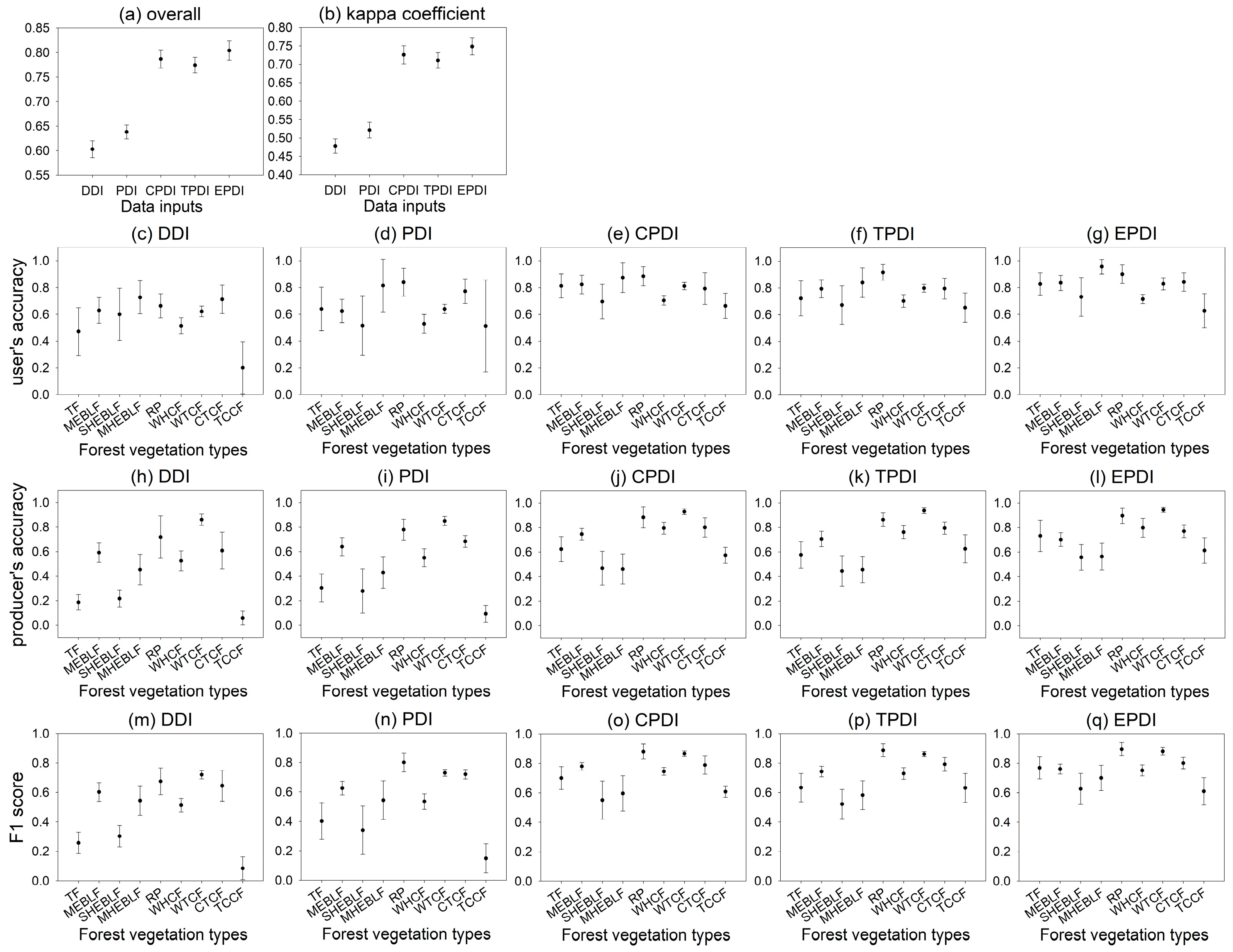
3.3. Mapping Accuracy Comparison

Phenological features significantly enhance the mapping accuracy of forest vegetation (

Table 2. Comparison of the average mapping accuracy using the F1 score, overall accuracy, and kappa coefficient across the five data inputs.

		DDI	PDI	PDI-DDI	CPDI-PDI	TPDI-PDI	EPDI-PDI
F1 score	TF	25.750%	40.163%	14.413%	29.862%	23.202%	36.723%
	MEBLF	60.312%	62.555%	2.244%	15.422%	11.741%	13.484%
	SHEBLF	30.327%	34.026%	3.699%	21.035%	18.159%	28.575%
	MHEBLF	54.492%	54.408%	−0.084%	5.160%	3.853%	15.613%
	RP	67.529%	80.127%	12.598%	7.923%	8.611%	9.446%
	WHCF	51.339%	53.502%	2.163%	21.041%	19.424%	21.645%
	WTCF	72.049%	72.935%	0.887%	13.660%	13.207%	15.221%
	CTCF	64.576%	71.989%	7.413%	6.857%	7.244%	8.139%
	TCCF	8.491%	14.893%	6.402%	45.899%	48.287%	46.050%
Overall accuracy (OA)		60.295%	63.825%	3.530%	14.845%	13.613%	16.583%
Kappa coefficient (KC)		47.800%	0.522%	4.341%	20.432%	18.902%	22.689%

, and Figure 5 and Figure 6). The DDI, which only considers spectral bands and vegetation indices during the defoliation period of RP, exhibited the lowest OA (0.603 ± 0.017) and KC (0.478 ± 0.019) compared to the other four data inputs. Incorporating spectral bands and vegetation indices from the refoliation period resulted in improvements of 3.530% in OA and 4.341% in KC for PDI. Specifically, the FS for TF, RP, CTCF, and TCCF in PDI improved by 14.413%, 12.598%, 7.413%, and 6.402%, respectively, compared to DDI (Table 2). Given that RP, CTCF, and TCCF exhibit significant temporal changes (Figure 3), the addition of phenological features enhances the mapping accuracy for these forest vegetation types.

Climatic and topographic variables also significantly improved the mapping accuracy of forest vegetation. The OA and KC for CPDI, TPDI, and EPDI improved by 14.845% and 20.432%, 13.613% and 18.902%, and 16.583% and 22.689%, respectively, compared to PDI. The FS for various forest vegetation types improved significantly with the inclusion of climatic or elevation variables to PDI. Notably, the FS for TF, MEBLF, SHEBLF, WHCF, WTCF, and TCCF in CPDI and TPDI improved by 29.862% and 23.202%, 15.422% and 11.741%, 21.035% and 18.159%, 21.041% and 19.424%, 13.660% and 13.207%, and 45.899% and 48.287%, respectively, compared to PDI. The FS of these forest vegetation types in CPDI and TPDI improved by more than 10% compared to PDI. Additionally, the FS for MHEBLF, RP, and CTCF of CPDI and TPDI also improved by approximately 5% compared to PDI. Furthermore, Table 2 and Figure 5 show that the FS for CTCF and TCCF in TPDI showed better separability than CPDI, with increases of 0.387% and 2.388%, respectively. The combination of climatic and topographic variables in EPDI resulted in the highest OA, KC, and FS values compared to PDI, CPDI, or TPDI. FS values for forest vegetation types in EPDI exceeded 0.6, with the FS of TF, MEBLF, SHEBLF, MHEBLF, RP, WHCF, WTCF, CTCF, and TCCF in EPDI improving by 36.723%, 13.484%, 28.575%, 15.613%, 9.446%, 21.645%, 15.221%, 8.139%, and 46.050%, respectively, compared to PDI.

The inclusion of phenological information and environmental variables led to better mapping accuracy and distribution in CPDI, TPDI, and EPDI compared to DDI and PDI (Figure 6). Forest vegetation distribution in DDI (Figure 6a) and PDI (Figure 6b) revealed misclassifications, with certain forest vegetation types (e.g., TF, MEBLF, WHTF, and RP) distributed at lower elevations being incorrectly classified into higher mountains or altitudes, such as the Hengduan Mountain Ranges in northwestern Yunnan (elevations greater than 2500 m). Conversely, some CTCF and TCCF at higher elevations were misclassified as lower elevation forests, particularly in southeastern Yunnan, while a portion of RP in TPDI was misclassified at higher altitudes in northeastern Yunnan compared with CPDI and EPDI (Figure 6d). Finally, CPDI and EPDI demonstrated better alignment with the actual vegetation distribution in Yunnan.

3.4. Characteristic of Historical Forest Vegetation Maps in Yunnan

We utilized the EPDI and MOD09A1.061 product to map the historical distribution of forest vegetation in Yunnan. The OA and KC of the forest historical maps in 2001, 2010, and 2020 were 77.021% and 0.704, 75.986% and 0.698, and 77.538% and 0.709, respectively.

Over the past 20 years, forest areas in Yunnan have shown an increasing trend (Figure 7). The forest area expanded from 19.957 × 10⁴ km² in 2001 to 20.736 × 10⁴ km² in 2011, and further to 22.026 × 10⁴ km² in 2020. However, various forest vegetation type groups exhibited varying changes in area during this period. TF decreased from 0.306 × 10⁴ km² in 2001 to 0.195 × 10⁴ km² in 2010, but increased to 0.313 × 10⁴ km² in 2020. Evergreen broad-leaved forests (including MEBLF, SHEBLF, and MHEBLF) rose from 4.264 × 10⁴ km² in 2001 to 5.672 × 10⁴ km² in 2020. RP increased from 0.292 × 10⁴ km² in 2001 to 0.731 × 10⁴ km² in 2010, and subsequently decreased to 0.691 × 10⁴ km² in 2020. Warm coniferous forests (including WHCF and WTCF) expanded from 12.523 × 10⁴ km² in 2001 to 12.840 × 10⁴ km² in 2020. In contrast, temperate coniferous forests (including CTCF and TCCF) at high elevations increased slightly from 2.572 × 10⁴ km² in 2001 to 2.577 × 10⁴ km² in 2010, and then decreased to 2.510 × 10⁴ km² in 2020.

4. Discussion

4.1. Spectral and Phenological Features in Differentiating Forest Vegetation Types

RP exhibits distinct phenological features that enable their differentiation through the inclusion of spectral bands and vegetation indices during defoliation and refoliation periods [20,21,51]. The significant reduction in canopy cover and leaf density of rubber during the defoliation period leads rubber to consume more stored water and carbohydrates [61,62]. This is consistent with our findings on phenological change in RP (Figure 3), where vegetation and water indices, such as NDVI, EVI, and LSWI, decrease with the decline in canopy cover and leaf density of rubber during the defoliation period, subsequently increasing during refoliation [21,62]. The difference in vegetation and water indices of rubber between defoliation and refoliation periods facilitates the spatial distribution of RP and its differentiation from evergreen broad-leaved forests and coniferous forests. Consistent with previous studies [20,62], we observed that LSWI, a moisture-related vegetation index, is particularly effective at distinguishing RP from other evergreen broad-leaved forests when compared to NDVI and EVI (Figure 4 and Table S1). Furthermore, snow cover affects LSWI values in CTCF and TCCF at high elevations from January to early March, resulting in higher LSWI readings during this period, compared to late March to May (Figure 3 and Figure 4). Water indices, such as LSWI, prove highly effective in distinguishing CTCF and TCCF from other forest vegetation types by detecting snow cover. Thus, we recommend incorporating water indices (e.g., LSWI) into vegetation mapping to detect differences in moisture among various vegetation types.

The disparities in leaf and canopy reflectance are crucial for distinguishing coniferous forests from broad-leaved forests. While most coniferous species lack pronounced phenological features (Figure 3) [63], their biochemistry traits of needle reflectance (e.g., needle water content and leaf chlorophyll), inner leaf structure, and canopy reflectance of coniferous species differ from those of broad-leaved forests [63]. Certain spectral and vegetation index differences are critical for distinguishing between coniferous and broad-leaved forests. Coniferous needles generally exhibit lower transmittance across all spectral bands and visible reflectance compared to broad leaves [63,64,65]. Our results support this, showing that visible bands are more effective at separating coniferous forests from broad-leaved forests (Figure 4 and Table S1). Additionally, we found EVI demonstrates superior separability compared to other vegetation indices (Figure 4k,o). Therefore, the strategic use of spectral bands and vegetation indices can effectively distinguish coniferous forests from broad-leaved forests.

4.2. The Role of Climatic and Topographic Information in Enhancing Forest Mapping Accuracy

Precipitation significantly influences the above-ground net primary production [66], species diversity, and community structure within forests [67]. Southern Yunnan, characterized by abundant precipitation, supports natural forest types such as TF and MEBLF, which exhibit higher above-ground net primary production and more complex community structures compared to SHEBLF, WTCF, CTCF, and TCCF distributed in northern Yunnan [68], where precipitation levels are relatively lower (Figure 4r). Secondary forest vegetation types of TF and MEBLF, such as RP and WHCF, can also be distinguished from SHEBLF and WTCF using precipitation data (Figure 4r and Table S2). While precipitation data enhance the separability between forest vegetation types with significant differences in above-ground net primary production, annual precipitation generally exhibits lower separability performance compared to annual mean temperature, particularly when distinguishing SHEBLF, MHEBLF, and WHCF from other types (Figure 4r and Table S2). This phenomenon may be attributed to the considerable annual precipitation in Yunnan, primarily influenced by the summer monsoon [42]. Several studies have indicated that in areas with low precipitation, precipitation variables play a more critical role in shaping vegetation structure and distribution [69,70].

Temperature distribution across forest vegetation types, influenced by latitude and altitude, also enhances forest mapping accuracy in Yunnan. As the primary factor affecting plant growth, distribution, and productivity [71], temperature varies across regions. For instance, tropical regions maintain higher mean temperatures, which optimize photosynthesis and metabolic rates [72], thereby forming tropical forests with greater biodiversity. In contrast, coniferous forests, primarily located in high-latitude and high-elevation areas, exhibit adaptations for cold resistance [73]. Each vegetation has its optimal temperature ranges [26], and these thermal zones delineate specific vegetation distributions [30]. In Yunnan, this results in natural and secondary forest vegetation types corresponding to different climatic zones: TF and RP in the tropics, MEBLF and WHCF in southern subtropical regions, SHEBLF and WTCF in northern subtropical zones, and CTCF and TCCF in temperate areas, leading to temperature variables’ enhanced separability of forest vegetation types (Figure 4q and Table S2).

Furthermore, temperature is negatively correlated with elevation [32], and distinct forest vegetation types occupy specific altitudinal ranges in montane regions (Table 1) [28]. Our findings aligned with previous studies demonstrate improved mapping accuracy in montane forests by combining elevation data with spectral images [33,34]. Notably, the inclusion of elevation information significantly improved the mapping accuracy of TPDI compared to PDI. However, topographic complexity can pose challenges to the mapping forest vegetation in Yunnan. For example, some RP were incorrectly mapped in lower elevations of northeastern Yunnan based on TPDI (Figure 6d), where the climate is unsuitable for RP growth. Although TPDI and CPDI exhibited similar OA and KC values, CPDI effectively reduced errors related to RP misclassification at lower elevations compared to TPDI (Figure 6c,d). The vertical distribution of forest vegetation presents significant potential for improving mapping accuracy in montane regions. Thus, we recommend leveraging climatic and topographic data to improve mapping accuracy in montane or large-scale areas.

4.3. Changes in Forest Area in Yunnan

The implementation of ecological policies has been a primary driver of improved forest cover in Yunnan, with our study revealing a 10.369% increase in forest area from 2001 to 2020. Since China launched the Grain for Green Program and the Natural Forest Protection Program in 1998 [60], significant enhancements in forest cover and ecosystem services have been observed across China [74,75]. Yunnan implemented these ecological policies starting in 2000 [43]. Predominantly coniferous species (e.g., Cunninghamia lanceolata, Pinus yunnanensis, and Pinus kesiya) and various broad-leaved species have been planted [43]. This aligns with our findings, which indicate the continuous growth in evergreen broad-leaved forests and warm coniferous forests (e.g., WHCF and WTCF) from 2001 to 2020. Furthermore, the Yunnan yearbooks from 2002 to 2021 document a total of 7.924 × 10⁴ km² afforested during 2001 to 2020, reinforcing our conclusion that forest area has exhibited an upward trend during this period. The increased forest cover may have improved ecosystem services in Yunnan over the past 20 years.

Conversely, human activities such as economic development and deforestation have affected the distribution of forest vegetation types in low-elevation areas of Yunnan. Previous studies have found that the expansion of RP was fueled by rising rubber prices from 2000 to 2010, followed by a subsequent decline in RP area due to falling rubber prices after 2010 [9,21,76]. Our findings corroborate this trend, showing an increase in RP from 2001 to 2010, followed by a decrease by 2020. Additionally, the area of TF in the low elevations of southern Yunnan decreased from 2001 to 2010, which might be related to forest losses associated with the RP expansion [9]. The interplay between the expansion of RP and the loss of TF in low elevations led to a degradation of ecosystem services in this region during this period [9]. In contrast, the subsequent reduction in RP area and the implementation of ecological programs contributed to a recovery in TF area in low elevations from 2010 to 2020 [9].

4.4. Applications and Limitations

This study demonstrates that integrating phenological information with multispectral bands effectively distinguishes various forest vegetation type groups. By incorporating climatic and topographic variables, and multispectral images, we achieved enhanced mapping accuracy for forest vegetation types compared to using multispectral images alone. In contrast to previous efforts, which involved extensive collaboration over more than a decade to produce a vegetation map of Yunnan at a scale of 1:2,000,000 in 1987 (Figure 1b) [28], our approach utilized only 948 POIs, alongside multispectral images, phenological features, and environmental variables, to generate similar spatial distribution patterns. This integration of multispectral images and environmental variables offers a more efficient and accurate method for vegetation mapping. Moreover, long-term land use maps facilitated the identification of unchanged POIs of forest vegetation types over the past two decades, allowing for the historical mapping of forest distribution in Yunnan. The reliance on long-term multispectral images, environmental variables, and POIs, enabled by Google Earth Engine [17], underscores the potential for this integrated approach in historical vegetation mapping.

Despite these strengths, this study has several limitations worth addressing. First, we focused solely on annual mean temperature, annual precipitation, and elevation to enhance mapping accuracy. Previous research has identified other critical environmental variables, such as minimum winter temperature, precipitation seasonality, and aridity index, as significant factors influencing vegetation structure and distribution [77,78,79]. Future vegetation mapping efforts should consider these limiting factors to further improve accuracy. Additionally, the limited number of ground reference data points resulted in the exclusion of five forest vegetation types and restricted our ability to assess mapping accuracy at the formation-type level. Future research should prioritize the collection of additional ground reference data to address these gaps.

5. Conclusions

Historical maps of forest vegetation are vital datasets for ecological assessment, protection, and management. In the current study, we employed the JMD method to compare the separability of nine major forest vegetation types in Yunnan. Our results revealed that RP can be distinguished from other forest vegetation types based on its phenological features, while coniferous and broad-leaved forests can be effectively distinguished through spectral differences. Additionally, climatic and elevation variables were found to effectively identify forest vegetation habitats with similar climate conditions. The inclusion of either climatic or elevation variables resulted in significant improvements in OA and KC for both CPDI and TPDI, compared to PDI. Notably, the EPDI achieved the highest mapping accuracy among the various data inputs. Therefore, we recommend incorporating phenological features alongside climatic and elevation variables for mapping forest vegetation distribution. Utilizing these variables, we successfully mapped historical forest vegetation in Yunnan for the years 2001, 2010, and 2020, revealing a 10.367% increase in forest area over this period, with evergreen broad-leaved forests contributing approximately two-thirds of this increase. The implementation of ecological policies is likely the primary reason for the improvement in the forest area in Yunnan. Our thematic maps can facilitate assessments of the ecological impacts of these policies and conservation efforts in Yunnan, aiding local ecological management decision-making in the future.

References

1. Bonan, G.B. Forests and Climate Change: Forcings, Feedbacks, and the Climate Benefits of Forests. Science 2008, 320, 1444–1449. [Google Scholar] [CrossRef]
2. Costanza, R.; d’Arge, R.; de Groot, R.; Farber, S.; Grasso, M.; Hannon, B.; Limburg, K.; Naeem, S.; O’Neill, R.V.; Paruelo, J.; et al. The value of the world’s ecosystem services and natural capital. Nature 1997, 387, 253–260. [Google Scholar] [CrossRef]
3. de Groot, R.; Brander, L.; van der Ploeg, S.; Costanza, R.; Bernard, F.; Braat, L.; Christie, M.; Crossman, N.; Ghermandi, A.; Hein, L.; et al. Global estimates of the value of ecosystems and their services in monetary units. Ecosyst. Serv. 2012, 1, 50–61. [Google Scholar] [CrossRef]
4. Yang, W.; Wang, Y.; Webb, A.A.; Li, Z.; Tian, X.; Han, Z.; Wang, S.; Yu, P. Influence of climatic and geographic factors on the spatial distribution of Qinghai spruce forests in the dryland Qilian Mountains of Northwest China. Sci. Total Environ. 2018, 612, 1007–1017. [Google Scholar] [CrossRef] [PubMed]
5. Zischg, A.P.; Frehner, M.; Gubelmann, P.; Augustin, S.; Brang, P.; Huber, B. Participatory modelling of upward shifts of altitudinal vegetation belts for assessing site type transformation in Swiss forests due to climate change. Appl. Veg. Sci. 2021, 24, e12621. [Google Scholar] [CrossRef]
6. Zhou, Y.; Yi, Y.-J.; Liu, H.-X.; Tang, C.-H.; Zhu, Y.-L.; Zhang, S.-H. Effect of geomorphologic features and climate change on vegetation distribution in the arid hot valleys of Jinsha River, Southwest China. J. Mt. Sci. 2022, 19, 2874–2885. [Google Scholar] [CrossRef]
7. Hua, F.; Xu, J.; Wilcove, D.S. A New Opportunity to Recover Native Forests in China. Conserv. Lett. 2018, 11, e12396. [Google Scholar] [CrossRef]
8. Hua, F.; Bruijnzeel, L.A.; Meli, P.; Martin, P.A.; Zhang, J.; Nakagawa, S.; Miao, X.; Wang, W.; McEvoy, C.; Peña-Arancibia, J.L.; et al. The biodiversity and ecosystem service contributions and trade-offs of forest restoration approaches. Science 2022, 376, 839–844. [Google Scholar] [CrossRef]
9. Yang, J.; Zhai, D.-L.; Fang, Z.; Alatalo, J.M.; Yao, Z.; Yang, W.; Su, Y.; Bai, Y.; Zhao, G.; Xu, J. Changes in and driving forces of ecosystem services in tropical southwestern China. Ecol. Indic. 2023, 149, 110180. [Google Scholar] [CrossRef]
10. Clark, M.L. Comparison of multi-seasonal Landsat 8, Sentinel-2 and hyperspectral images for mapping forest alliances in Northern California. ISPRS-J. Photogramm. Remote Sens. 2020, 159, 26–40. [Google Scholar] [CrossRef]
11. Zhang, Z.; Lu, L.; Zhao, Y.; Wang, Y.; Wei, D.; Wu, X.; Ma, X. Recent advances in using Chinese Earth observation satellites for remote sensing of vegetation. ISPRS-J. Photogramm. Remote Sens. 2023, 195, 393–407. [Google Scholar] [CrossRef]
12. Ghosh, A.; Fassnacht, F.E.; Joshi, P.K.; Koch, B. A framework for mapping tree species combining hyperspectral and LiDAR data: Role of selected classifiers and sensor across three spatial scales. Int. J. Appl. Earth Obs. Geoinf. 2014, 26, 49–63. [Google Scholar] [CrossRef]
13. Mäyrä, J.; Keski-Saari, S.; Kivinen, S.; Tanhuanpää, T.; Hurskainen, P.; Kullberg, P.; Poikolainen, L.; Viinikka, A.; Tuominen, S.; Kumpula, T.; et al. Tree species classification from airborne hyperspectral and LiDAR data using 3D convolutional neural networks. Remote Sens. Environ. 2021, 256, 112322. [Google Scholar] [CrossRef]
14. Iglseder, A.; Immitzer, M.; Dostálová, A.; Kasper, A.; Pfeifer, N.; Bauerhansl, C.; Schöttl, S.; Hollaus, M. The potential of combining satellite and airborne remote sensing data for habitat classification and monitoring in forest landscapes. Int. J. Appl. Earth Obs. Geoinf. 2023, 117, 103131. [Google Scholar] [CrossRef]
15. Hu, T.; Zhang, Y.; Su, Y.; Zheng, Y.; Lin, G.; Guo, Q. Mapping the Global Mangrove Forest Aboveground Biomass Using Multisource Remote Sensing Data. Remote Sens. 2020, 12, 1690. [Google Scholar] [CrossRef]
16. Wulder, M.A.; Masek, J.G.; Cohen, W.B.; Loveland, T.R.; Woodcock, C.E. Opening the archive: How free data has enabled the science and monitoring promise of Landsat. Remote Sens. Environ. 2012, 122, 2–10. [Google Scholar] [CrossRef]
17. Gorelick, N.; Hancher, M.; Dixon, M.; Ilyushchenko, S.; Thau, D.; Moore, R. Google Earth Engine: Planetary-scale geospatial analysis for everyone. Remote Sens. Environ. 2017, 202, 18–27. [Google Scholar] [CrossRef]
18. Zeng, L.; Wardlow, B.D.; Xiang, D.; Hu, S.; Li, D. A review of vegetation phenological metrics extraction using time-series, multispectral satellite data. Remote Sens. Environ. 2020, 237, 111511. [Google Scholar] [CrossRef]
19. Xue, Z.; Du, P.; Feng, L. Phenology-Driven Land Cover Classification and Trend Analysis Based on Long-term Remote Sensing Image Series. IEEE J. Sel. Top. Appl. Earth Observ. Remote Sens. 2014, 7, 1142–1156. [Google Scholar] [CrossRef]
20. Zhai, D.; Dong, J.; Cadisch, G.; Wang, M.; Kou, W.; Xu, J.; Xiao, X.; Abbas, S. Comparison of Pixel- and Object-Based Approaches in Phenology-Based Rubber Plantation Mapping in Fragmented Landscapes. Remote Sens. 2018, 10, 44. [Google Scholar] [CrossRef]
21. Yang, J.; Xu, J.; Zhai, D.-L. Integrating Phenological and Geographical Information with Artificial Intelligence Algorithm to Map Rubber Plantations in Xishuangbanna. Remote Sens. 2021, 13, 2793. [Google Scholar] [CrossRef]
22. Senf, C.; Laštovička, J.; Okujeni, A.; Heurich, M.; van der Linden, S. A generalized regression-based unmixing model for mapping forest cover fractions throughout three decades of Landsat data. Remote Sens. Environ. 2020, 240, 111691. [Google Scholar] [CrossRef]
23. Guo, J.; Du, S. A Multicenter Soft Supervised Classification Method for Modeling Spectral Diversity in Multispectral Remote Sensing Data. IEEE Trans. Geosci. Remote Sens. 2022, 60, 5605517. [Google Scholar] [CrossRef]
24. Woodward, F.I.; Lomas, M.R.; Kelly, C.K. Global Climate and the Distribution of Plant Biomes. Philos. Trans. R. Soc. B-Biol. Sci. 2004, 359, 1465–1476. [Google Scholar] [CrossRef] [PubMed]
25. Barga, S.C.; Dilts, T.E.; Leger, E.A. Contrasting climate niches among co-occurring subdominant forbs of the sagebrush steppe. Divers. Distrib. 2018, 24, 1291–1307. [Google Scholar] [CrossRef]
26. Sun, G.-Q.; Li, L.; Li, J.; Liu, C.; Wu, Y.-P.; Gao, S.; Wang, Z.; Feng, G.-L. Impacts of climate change on vegetation pattern: Mathematical modeling and data analysis. Phys. Life Rev. 2022, 43, 239–270. [Google Scholar] [CrossRef]
27. Li, F.-F.; Lu, H.-L.; Wang, G.-Q.; Yao, Z.-Y.; Li, Q.; Qiu, J. Zoning of precipitation regimes on the Qinghai–Tibet Plateau and its surrounding areas responded by the vegetation distribution. Sci. Total Environ. 2022, 838, 155844. [Google Scholar] [CrossRef]
28. Wu, Z. Vegetation of Yunnan; Science Press: Beijing, China, 1987; pp. 81–417. [Google Scholar]
29. Fang, J.; Song, Y.; Liu, H.; Piao, S. Vegetation-climate relationship and its application in the division of vegetation zone in China. Acta Bot. Sin. 2002, 44, 1105–1122. [Google Scholar]
30. Fang, J.-y.; Yoda, K. Climate and vegetation in China II. Distribution of main vegetation types and thermal climate. Ecol. Res. 1989, 4, 71–83. [Google Scholar] [CrossRef]
31. Lin, H.-Y.; Li, C.-F.; Chen, T.-Y.; Hsieh, C.-F.; Wang, G.; Wang, T.; Hu, J.-M. Climate-based approach for modeling the distribution of montane forest vegetation in Taiwan. Appl. Veg. Sci. 2020, 23, 239–253. [Google Scholar] [CrossRef]
32. Shao, J.a.; Li, Y.; Ni, J. The characteristics of temperature variability with terrain, latitude and longitude in Sichuan-Chongqing Region. J. Geogr. Sci. 2012, 22, 223–244. [Google Scholar] [CrossRef]
33. Zhu, X.; Liu, D. Accurate mapping of forest types using dense seasonal Landsat time-series. ISPRS-J. Photogramm. Remote Sens. 2014, 96, 1–11. [Google Scholar] [CrossRef]
34. Hościło, A.; Lewandowska, A. Mapping Forest Type and Tree Species on a Regional Scale Using Multi-Temporal Sentinel-2 Data. Remote Sens. 2019, 11, 929. [Google Scholar] [CrossRef]
35. Fick, S.E.; Hijmans, R.J. WorldClim 2: New 1-km spatial resolution climate surfaces for global land areas. Int. J. Climatol. 2017, 37, 4302–4315. [Google Scholar] [CrossRef]
36. Okolie, C.J.; Smit, J.L. A systematic review and meta-analysis of Digital elevation model (DEM) fusion: Pre-processing, methods and applications. ISPRS-J. Photogramm. Remote Sens. 2022, 188, 1–29. [Google Scholar] [CrossRef]
37. Riley, K.L.; Grenfell, I.C.; Finney, M.A. Mapping forest vegetation for the western United States using modified random forests imputation of FIA forest plots. Ecosphere 2016, 7, e01472. [Google Scholar] [CrossRef]
38. Zhou, G.; Ren, H.; Liu, T.; Zhou, L.; Ji, Y.; Song, X.; Lv, X. A new regional vegetation mapping method based on terrain-climate-remote sensing and its application on the Qinghai-Xizang Plateau. Sci. China-Earth Sci. 2023, 66, 237–246. [Google Scholar] [CrossRef]
39. Wu, F.; Ren, H.; Zhou, G. The 30 m vegetation maps from 1990 to 2020 in the Tibetan Plateau. Sci. Data 2024, 11, 804. [Google Scholar] [CrossRef]
40. Reddy, C.S.; Jha, C.S.; Diwakar, P.G.; Dadhwal, V.K. Nationwide classification of forest types of India using remote sensing and GIS. Environ. Monit. Assess. 2015, 187, 777. [Google Scholar] [CrossRef]
41. Su, Y.; Guo, Q.; Hu, T.; Guan, H.; Jin, S.; An, S.; Chen, X.; Guo, K.; Hao, Z.; Hu, Y.; et al. An updated Vegetation Map of China (1:1,000,000). Sci. Bull. 2020, 65, 1125–1136. [Google Scholar] [CrossRef]
42. Yang, Y.; Tian, K.; Hao, J.; Pei, S.; Yang, Y. Biodiversity and biodiversity conservation in Yunnan, China. Biodivers. Conserv. 2004, 13, 813–826. [Google Scholar] [CrossRef]
43. Chen, X.; Zhang, X.; Zhang, Y.; Wan, C. Carbon sequestration potential of the stands under the Grain for Green Program in Yunnan Province, China. For. Ecol. Manag. 2009, 258, 199–206. [Google Scholar] [CrossRef]
44. Zhou, R.; Li, W.; Zhang, Y.; Peng, M.; Wang, C.; Sha, L.; Liu, Y.; Song, Q.; Fei, X.; Jin, Y.; et al. Responses of the Carbon Storage and Sequestration Potential of Forest Vegetation to Temperature Increases in Yunnan Province, SW China. Forests 2018, 9, 227. [Google Scholar] [CrossRef]
45. Peng, J.; Yang, Y.; Liu, Y.; Hu, Y.n.; Du, Y.; Meersmans, J.; Qiu, S. Linking ecosystem services and circuit theory to identify ecological security patterns. Sci. Total Environ. 2018, 644, 781–790. [Google Scholar] [CrossRef]
46. Zhu, H.; Tan, Y. Flora and Vegetation of Yunnan, Southwestern China: Diversity, Origin and Evolution. Diversity 2022, 14, 340. [Google Scholar] [CrossRef]
47. Hua, Z. Biogeographical Divergence of the Flora of Yunnan, Southwestern China Initiated by the Uplift of Himalaya and Extrusion of Indochina Block. PLoS ONE 2012, 7, e45601. [Google Scholar] [CrossRef]
48. Hua, Z. Advances in Biogeography of the Tropical Rain Forest in Southern Yunnan, Southwestern China. Trop. Conserv. Sci. 2008, 1, 34–42. [Google Scholar] [CrossRef]
49. Zhang, M.-G.; Zhou, Z.-K.; Chen, W.-Y.; Slik, J.W.F.; Cannon, C.H.; Raes, N. Using species distribution modeling to improve conservation and land use planning of Yunnan, China. Biol. Conserv. 2012, 153, 257–264. [Google Scholar] [CrossRef]
50. Wu, Q. geemap: A Python package for interactive mapping with Google Earth Engine. J. Open Source Softw. 2020, 5, 2305. [Google Scholar] [CrossRef]
51. Wang, Y.; Hollingsworth, P.M.; Zhai, D.; West, C.D.; Green, J.M.H.; Chen, H.; Hurni, K.; Su, Y.; Warren-Thomas, E.; Xu, J.; et al. High-resolution maps show that rubber causes substantial deforestation. Nature 2023, 623, 340–346. [Google Scholar] [CrossRef]
52. Huete, A.; Didan, K.; Miura, T.; Rodriguez, E.P.; Gao, X.; Ferreira, L.G. Overview of the radiometric and biophysical performance of the MODIS vegetation indices. Remote Sens. Environ. 2002, 83, 195–213. [Google Scholar] [CrossRef]
53. Defries, R.S.; Townshend, J.R.G. NDVI-derived land cover classifications at a global scale. Int. J. Remote Sens. 1994, 15, 3567–3586. [Google Scholar] [CrossRef]
54. Xiao, X.; Boles, S.; Liu, J.; Zhuang, D.; Frolking, S.; Li, C.; Salas, W.; Moore, B. Mapping paddy rice agriculture in southern China using multi-temporal MODIS images. Remote Sens. Environ. 2005, 95, 480–492. [Google Scholar] [CrossRef]
55. Yang, R.-Q.; Fu, P.-L.; Fan, Z.-X.; Panthi, S.; Gao, J.; Niu, Y.; Li, Z.-S.; Bräuning, A. Growth-climate sensitivity of two pine species shows species-specific changes along temperature and moisture gradients in southwest China. Agric. For. Meteorol. 2022, 318, 108907. [Google Scholar] [CrossRef]
56. Farr, T.G.; Rosen, P.A.; Caro, E.; Crippen, R.; Duren, R.; Hensley, S.; Kobrick, M.; Paller, M.; Rodriguez, E.; Roth, L.; et al. The Shuttle Radar Topography Mission. Rev. Geophys. 2007, 45, RG2004. [Google Scholar] [CrossRef]
57. Yang, J.; Xu, J.; Zhou, Y.; Zhai, D.; Chen, H.; Li, Q.; Zhao, G. Paddy Rice Phenological Mapping throughout 30-Years Satellite Images in the Honghe Hani Rice Terraces. Remote Sens. 2023, 15, 2398. [Google Scholar] [CrossRef]
58. Jung, R.; Ehlers, M. Comparison of two feature selection methods for the separability analysis of intertidal sediments with spectrometric datasets in the German Wadden Sea. Int. J. Appl. Earth Obs. Geoinf. 2016, 52, 175–191. [Google Scholar] [CrossRef]
59. Belgiu, M.; Drăguţ, L. Random forest in remote sensing: A review of applications and future directions. ISPRS-J. Photogramm. Remote Sens. 2016, 114, 24–31. [Google Scholar] [CrossRef]
60. Liu, J.; Li, S.; Ouyang, Z.; Tam, C.; Chen, X. Ecological and socioeconomic effects of China’s policies for ecosystem services. Proc. Natl. Acad. Sci. USA 2008, 105, 9477–9482. [Google Scholar] [CrossRef]
61. Zhai, D.-L.; Xu, J.-C. The legacy effects of rubber defoliation period on the refoliation phenology, leaf disease, and latex yield. Plant Divers. 2023, 45, 98–103. [Google Scholar] [CrossRef]
62. Chen, B.; Li, X.; Xiao, X.; Zhao, B.; Dong, J.; Kou, W.; Qin, Y.; Yang, C.; Wu, Z.; Sun, R.; et al. Mapping tropical forests and deciduous rubber plantations in Hainan Island, China by integrating PALSAR 25-m and multi-temporal Landsat images. Int. J. Appl. Earth Obs. Geoinf. 2016, 50, 117–130. [Google Scholar] [CrossRef]
63. Rautiainen, M.; Lukeš, P.; Homolová, L.; Hovi, A.; Pisek, J.; Mõttus, M. Spectral Properties of Coniferous Forests: A Review of In Situ and Laboratory Measurements. Remote Sens. 2018, 10, 207. [Google Scholar] [CrossRef]
64. Lukeš, P.; Stenberg, P.; Rautiainen, M.; Mõttus, M.; Vanhatalo, K.M. Optical properties of leaves and needles for boreal tree species in Europe. Remote Sens. Lett. 2013, 4, 667–676. [Google Scholar] [CrossRef]
65. Roberts, D.A.; Ustin, S.L.; Ogunjemiyo, S.; Greenberg, J.; Dobrowski, S.Z.; Chen, J.; Hinckley, T.M. Spectral and Structural Measures of Northwest Forest Vegetation at Leaf to Landscape Scales. Ecosystems 2004, 7, 545–562. [Google Scholar] [CrossRef]
66. Robinson, T.M.P.; La Pierre, K.J.; Vadeboncoeur, M.A.; Byrne, K.M.; Thomey, M.L.; Colby, S.E. Seasonal, not annual precipitation drives community productivity across ecosystems. Oikos 2013, 122, 727–738. [Google Scholar] [CrossRef]
67. Hiltner, U.; Bräuning, A.; Gebrekirstos, A.; Huth, A.; Fischer, R. Impacts of precipitation variability on the dynamics of a dry tropical montane forest. Ecol. Model. 2016, 320, 92–101. [Google Scholar] [CrossRef]
68. Chen, X.; Zhang, Y. Impacts of climate, phenology, elevation and their interactions on the net primary productivity of vegetation in Yunnan, China under global warming. Ecol. Indic. 2023, 154, 110533. [Google Scholar] [CrossRef]
69. Otto, R.; Fernández-Palacios, J.M.; Krüsi, B.O. Variation in species composition and vegetation structure of succulent scrub on Tenerife in relation to environmental variation. J. Veg. Sci. 2001, 12, 237–248. [Google Scholar] [CrossRef]
70. Zheng, Y.; Xie, Z.; Jiang, L.; Shimizu, H.; Rimmington, G.M.; Zhou, G. Vegetation responses along environmental gradients on the Ordos plateau, China. Ecol. Res. 2006, 21, 396–404. [Google Scholar] [CrossRef]
71. Ding, Y.; Shi, Y.; Yang, S. Molecular Regulation of Plant Responses to Environmental Temperatures. Mol. Plant. 2020, 13, 544–564. [Google Scholar] [CrossRef]
72. Doughty, C.E.; Keany, J.M.; Wiebe, B.C.; Rey-Sanchez, C.; Carter, K.R.; Middleby, K.B.; Cheesman, A.W.; Goulden, M.L.; da Rocha, H.R.; Miller, S.D.; et al. Tropical forests are approaching critical temperature thresholds. Nature 2023, 621, 105–111. [Google Scholar] [CrossRef] [PubMed]
73. Zhao, C.; Li, X.; Zhou, X.; Zhao, K.; Yang, Q. Holocene Vegetation Succession and Response to Climate Change on the South Bank of the Heilongjiang-Amur River, Mohe County, Northeast China. Adv. Meteorol. 2016, 2016, 2450697. [Google Scholar] [CrossRef]
74. Ouyang, Z.; Zheng, H.; Xiao, Y.; Polasky, S.; Liu, J.; Xu, W.; Wang, Q.; Zhang, L.; Xiao, Y.; Rao, E.; et al. Improvements in ecosystem services from investments in natural capital. Science 2016, 352, 1455–1459. [Google Scholar] [CrossRef] [PubMed]
75. Chen, C.; Park, T.; Wang, X.; Piao, S.; Xu, B.; Chaturvedi, R.K.; Fuchs, R.; Brovkin, V.; Ciais, P.; Fensholt, R.; et al. China and India lead in greening of the world through land-use management. Nat. Sustain. 2019, 2, 122–129. [Google Scholar] [CrossRef] [PubMed]
76. Zhang, J.-Q.; Corlett, R.T.; Zhai, D. After the rubber boom: Good news and bad news for biodiversity in Xishuangbanna, Yunnan, China. Reg. Envir. Chang. 2019, 19, 1713–1724. [Google Scholar] [CrossRef]
77. Kavgacı, A.; Balpınar, N.; Öner, H.H.; Arslan, M.; Bonari, G.; Chytrý, M.; Čarni, A. Classification of forest and shrubland vegetation in Mediterranean Turkey. Appl. Veg. Sci. 2021, 24, e12589. [Google Scholar] [CrossRef]
78. Gao, N.; Guan, T.; Zhou, J.; Cai, W.; Zhang, X.; Li, H.; Jiang, L.; Zheng, Y. Vegetation patterns and causal factors in different reaches of an endorheic basin in arid China. Écoscience 2019, 26, 71–83. [Google Scholar] [CrossRef]
79. Bueno, M.L.; Rezende, V.L.; Pontara, V.; de Oliveira-Filho, A.T. Floristic distributional patterns in a diverse ecotonal area in South America. Plant Ecol. 2017, 218, 1171–1186. [Google Scholar] [CrossRef]
Figure 1. (a) Location of Yunnan within China; (b) major forest vegetation distribution in 1987 (mapped by Prof. Hua Zhu, Xishuangbanna Tropical Botanical Garden, CAS based on Vegetation of Yunnan (1987)); (c) elevation ranges of Yunnan and distribution of points of interest (POIs).
Remotesensing 16 03687 g001
Figure 2. Workflow for mapping forest vegetation in Yunnan.
Remotesensing 16 03687 g002
Figure 3. The time series of LSWI and EVI indices for nine forest vegetation types, calculated from the MOD09A1.061 product in 2015. The values represent the average from 25 POIs for each forest vegetation type. Abbreviations: DOY, day of the year.
Remotesensing 16 03687 g003
Figure 4. Box plots of spectral bands (blue, green, red, NIR, and SWIR1) and vegetation indices (NDVI, EVI, and LSWI) during defoliation and refoliation periods, and environmental variables (annual mean temperature, annual precipitation, and elevation) across nine forest vegetation types: (a) blue band during defoliation period; (b) green band during defoliation period; (c) red band during defoliation period; (d) NIR band during defoliation period; (e) blue band during refoliation period; (f) green band during refoliation period; (g) red band during refoliation period; (h) NIR band during refoliation period; (i) SWIR1 band during defoliation period; (j) NDVI during defoliation period; (k) EVI during defoliation period; (l) LSWI during defoliation period; (m) SWIR1 band during refoliation period; (n) NDVI during refoliation period; (o) EVI during refoliation period; (p) LSWI during refoliation period; (q) annual mean temperature; (r) annual precipitation; (s) elevation. Abbreviations: TF, tropical forest; MEBLF, monsoon evergreen broad-leaved forest; SHEBLF, semi-humid evergreen broad-leaved forest; MHEBLF, mountainous humid evergreen broad-leaved forest; RP, rubber plantation; WHCF, warm-hot coniferous forest; WTCF, warm-temperate coniferous forest; CTCF, cold-temperate coniferous forest; TCCF, temperate-cool coniferous forest.
Remotesensing 16 03687 g004
Figure 5. Mapping accuracy results: (a) overall accuracy, (b) kappa coefficient, (cg) user’s accuracy, (h,i) producer’s accuracy, and (mq) F1 score. DDI, PDI, CPDI, TPDI, and EPDI represent the five data inputs.
Remotesensing 16 03687 g005
Figure 6. Comparison of forest classifications in 2015 across five data inputs. Abbreviations: NF, non-forest lands; OA, overall accuracy; KC, kappa coefficient.
Remotesensing 16 03687 g006
Figure 7. The distributions of forest vegetation types: (a) 2001, (b) 2010, (c) 2020, and (d) the area changes of forest vegetation types in 2001, 2010, and 2020.
Remotesensing 16 03687 g007