Article

Improving Aboveground Biomass Estimation in Lowland Tropical Forests across Aspect and Age Stratification: A Case Study in Xishuangbanna

1
Key Laboratory of State Administration of Forestry and Grassland on Biodiversity Conservation in Southwest China, Southwest Forestry University, Kunming 650233, China
2
Key Laboratory for Forest Resources Conservation and Utilization in the Southwest Mountains of China, Ministry of Education, Southwest Forestry University, Kunming 650233, China
3
Yunnan Institute of Forest Inventory and Planning, Kunming 650051, China
4
Institute of Big Data and Artificial Intelligence, Southwest Forestry University, Kunming 650224, China
*
Author to whom correspondence should be addressed.
Remote Sens. 2024, 16(7), 1276; https://doi.org/10.3390/rs16071276
Submission received: 25 February 2024 / Revised: 31 March 2024 / Accepted: 3 April 2024 / Published: 4 April 2024

Abstract

:
Improving the precision of aboveground biomass (AGB) estimation in lowland tropical forests is crucial to enhancing our understanding of carbon dynamics and formulating climate change mitigation strategies. This study proposes an AGB estimation method for lowland tropical forests in Xishuangbanna, which include various vegetation types, such as Pinus kesiya var. langbianensis, oak, Hevea brasiliensis, and other broadleaf trees. In this study, 2016 forest management inventory data are integrated with remote sensing variables from Landsat 8 OLI (L8) and Sentinel 2A (S2) imagery to estimate forest AGB. The forest age and aspect were utilized as stratified variables to construct the random forest (RF) models, which may improve the AGB estimation accuracy. The key findings are as follows: (1) through variable screening, elevation was identified as the main factor correlated with the AGB, with texture measures derived from a pixel window size of 7 × 7 perform best for AGB sensitivity, followed by 5 × 5, with 3 × 3 being the least effective. (2) A comparative analysis of imagery groups for the AGB estimation revealed that combining L8 and S2 imagery achieved superior performance over S2 imagery alone, which, in turn, surpassed the accuracy of L8 imagery. (3) Stratified models, which integrated aspect and age variables, consistently outperformed the unstratified models, offering a more refined fit for lowland tropical forest AGB estimation. (4) Among the analyzed forest types, the AGB of P. kesiya var. langbianensis forests was estimated with the highest accuracy, followed by H. brasiliensis, oak, and other broadleaf forests within the RF models. These findings highlight the importance of selecting appropriate variables and sensor combinations in addition to the potential of stratified modeling approaches to improve the precision of forest biomass estimation. Overall, incorporating stratification theory and multi-source data can enhance the AGB estimation accuracy in lowland tropical forests, thus offering crucial insights for refining forest management strategies.

1. Introduction

Forests play a crucial role in regulating global carbon and water cycles [1]. In this context, accurately estimating aboveground biomass (AGB) is essential for understanding the ecological functions of forests and providing an informed basis for sustainable forest management practices [2]. Traditional field-based methods for AGB estimation are often time-consuming, costly, and limited in their spatial coverage. In recent years, remote sensing techniques, especially those using optical sensors, have been widely applied to forest AGB estimation due to the advantages of their wide spatial coverage, cost-effectiveness, and non-invasive nature [3,4]. However, significant challenges remain in terms of improving the accuracy of forest AGB estimation using remote sensing data [5,6].
Optical remote sensing data, especially Landsat 8 Operational Land Imager (L8) and Sentinel 2A (S2) imagery, have proven effective for forest AGB estimation due to the strong correlations between their spectral bands and AGB [3,6,7]. Imran and Ahmed [8] and Li et al. [9] demonstrated the effectiveness of L8 imagery in estimating forest biomass and carbon stocks. Tang et al. [5] found that using L8 imagery and sample data can better estimate the AGB of three common pine forests (Pinus yunnanensis forests, Pinus densata forests, and Pinus kesiya forests) in Yunnan Province. While the L8 provides freely available surface observation data, its applications in some scenarios are limited by its maximum resolution (30 m), which can be effectively addressed by using freely available S2 data [10]. For example, one study presented an effective AGB estimation method for buffer zone forests in Nepal using S2 data based on the random forest (RF) approach, highlighting the viability of S2 as a hyperspectral data alternative [11].
Despite the strengths of these data, there are some accuracy and generalizability limitations when using single-source remote sensing data to estimate forest AGB, which can be addressed by employing multi-source remote sensing data to enhance the precision and applicability of AGB estimation [12,13]. Multi-source remote sensing data have been widely used in previous studies to estimate forest AGB [3,14]. For example, Huang et al. [15] highlighted the impact of selecting appropriate variables and machine learning models on accurately estimating AGB using L8 and S2 imagery for mixed forests in Yunnan. Sa and Fan [16] proposed an approach to improve forest quality and carbon stock assessment by integrating L8 and S2 data, in which they used spectral indices and texture analysis to enhance vegetation parameter estimation. Overall, the use of multi-source remote sensing offers integrated, high-resolution, temporally rich, accurate, and consistent data, which can improve the AGB estimation accuracy [13,17]. In addition, various studies have also used band combinations, vegetation indices, image transformations, and texture characteristics to further enhance the forest AGB estimation accuracy [18,19].
In addition to classical approaches, machine learning models are also widely used in forest AGB estimation [20]. For example, Li et al. [21] enhanced forest biomass estimation in China by combining National Forest Inventory and L8 data with algorithms including linear regression, RF, and XGBoost. Their results highlighted the importance of variable selection and the performance of machine learning, especially the RF model, for accurately modeling AGB by forest type. Karlson et al. [22] showed that L8 data, combined with RF models and optimized variables, were able to accurately map AGB in Burkina Faso, offering a viable, data-accessible method for woodland analysis. Another study achieved superior accuracy in forest AGB estimation across diverse ecosystems using the RF model, with multispectral satellite data and advanced variable selection techniques used to effectively characterize the forest’s spatial distribution and complexity [23]. Some studies have also suggested that RF models are typically more resilient to outliers and noise, as well as more robust [24]. Therefore, given its robustness and precision, the RF model is the preferred bagging learner for forest AGB estimation [6].
Furthermore, vegetation age and aspect have important impacts on biomass allocation and distribution, as these parameters directly influence forest structure and productivity [25]. Ou et al. [26] incorporated stand age as a dummy variable in their study, which significantly enhanced the AGB estimation accuracy of Pinus densata forests. The accuracy of forest AGB estimation can be improved by considering the stratification of vegetation types and/or aspects [27]. In addition, Chen et al. [28] investigated AGB estimation for bamboo forests in Zhejiang with S2 data and identified spectral variations by growth stage; however, their analysis was affected by data saturation issues. This suggests that integrating diverse imagery and variable stratification are potentially suitable approaches to achieve improved accuracy when analyzing forest AGB. Additionally, lowland tropical forests, recognized for their biodiversity, play a crucial role in global carbon storage [29]. A key representative example of this ecosystem type is Xishuangbanna, China [30], which has important biodiversity, ecological roles, climate influence, and cultural significance.
Overall, there have been few studies to date on estimating forest AGB that consider aspect and age as stratified variables, the inclusion of which may improve AGB estimation accuracy in lowland forests. To address this research gap, in this study, the forest AGB was calculated from the forest management inventory (FMI) data from 2016, and contemporaneous L8 and S2 imagery were utilized to extract various types of remote sensing variables. The forest AGB and selected variables were then used to develop an RF model, with forest age and aspect chosen as stratification variables to improve estimation accuracy. The objectives of this study are as follows:
(1)
To explore the efficacy of L8, S2, and L8 + S2 classes in estimating lowland tropical forest AGB.
(2)
To explore improvements in AGB estimation through aspect and age stratification in RF models.

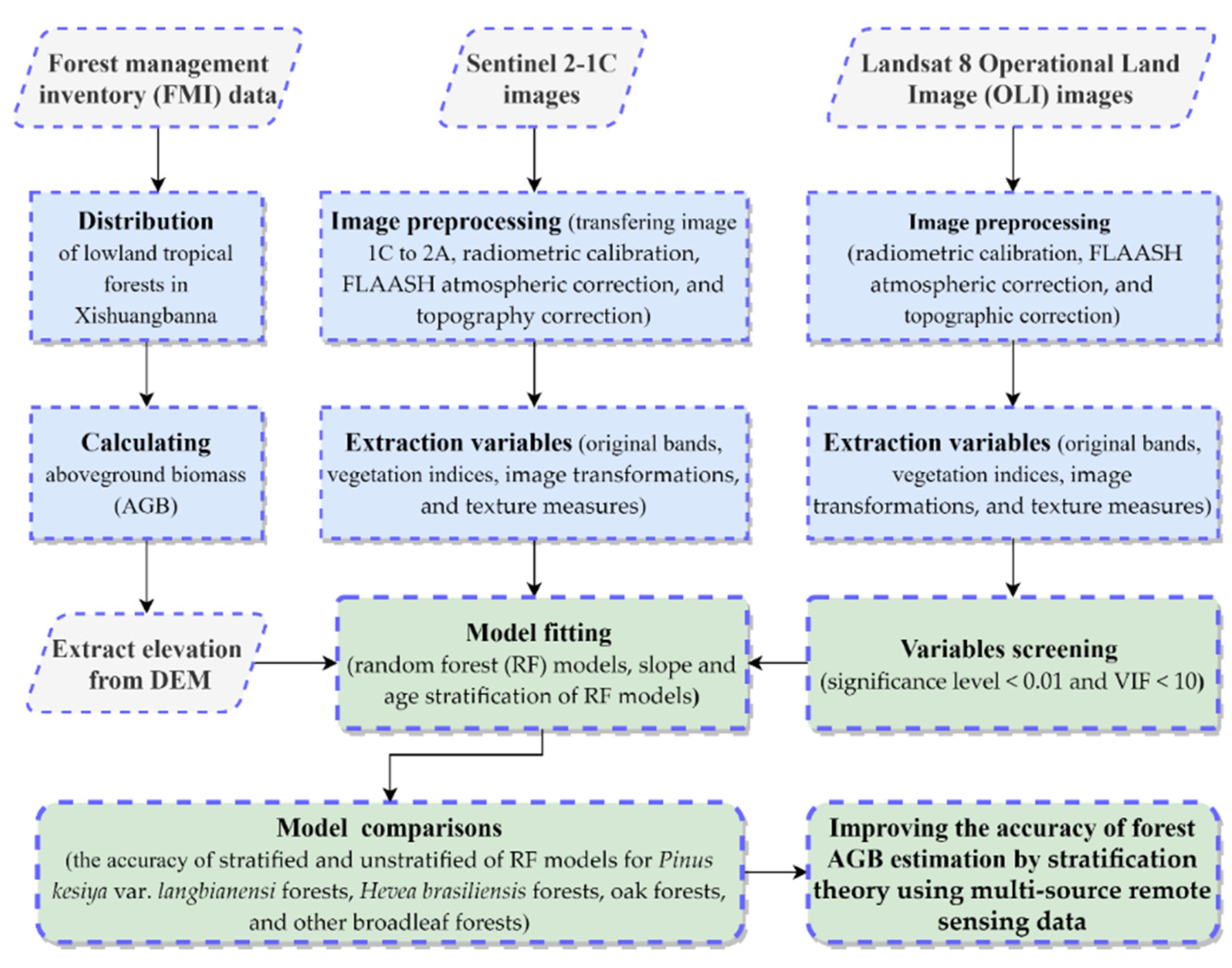
2. Materials and Methods
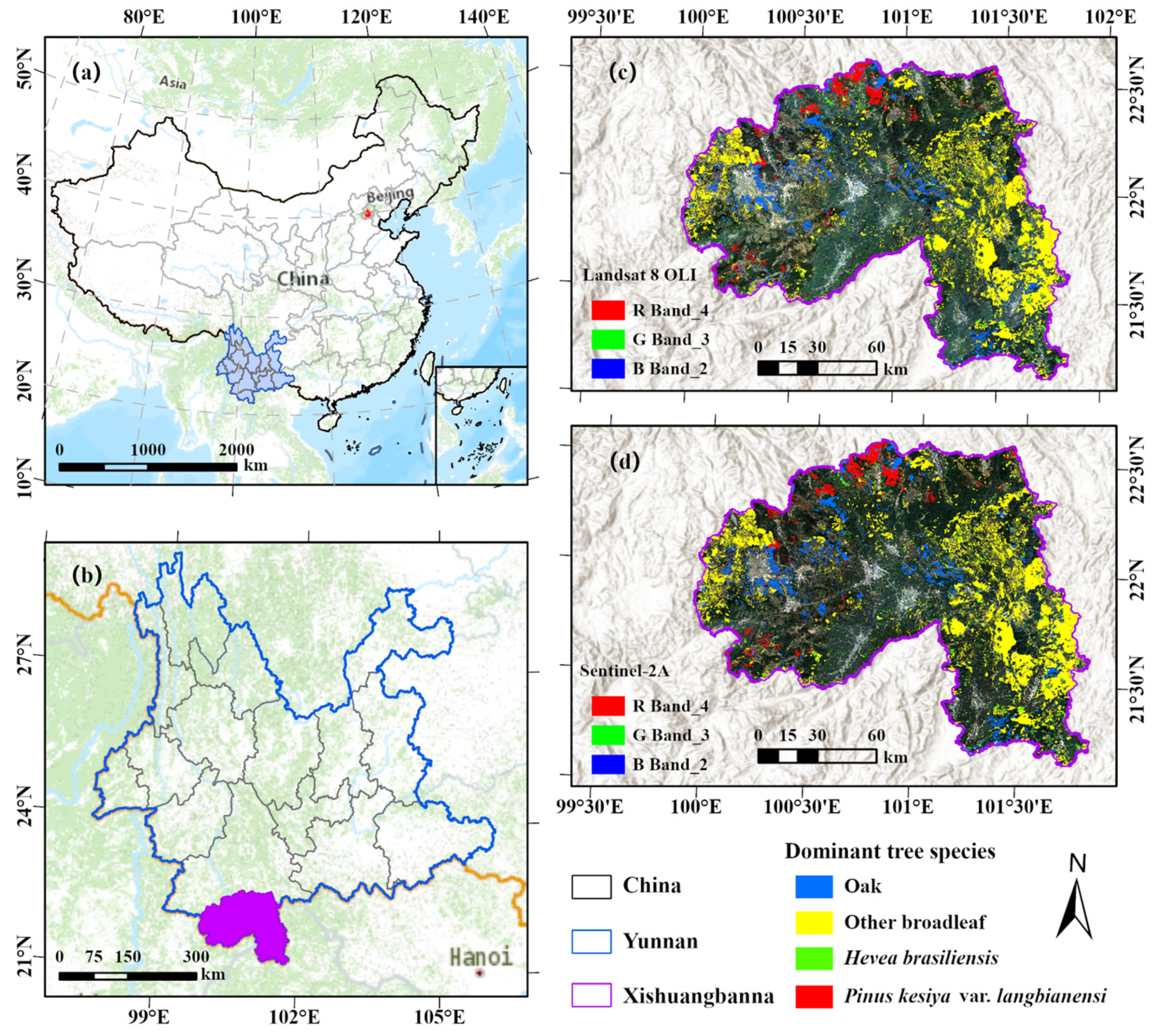
The methodological framework of this study is shown in Figure 1, the main steps of which are as follows: (1) obtaining the distribution of various forest types from FMI data; (2) calculating the forest AGB; (3) acquiring and processing L8 and S2 imagery; (4) extracting the original bands, vegetation indices, image transformations, and texture measures from L8 and S2 imagery; (5) screening variables for significance level <0.01 and variance inflation factor (VIF) <10 relative to forest AGB; (6) constructing RF models with aspect and age stratification; (7) comparing the accuracy of stratified and unstratified RF models; and (8) examining how stratification theory affects estimating forest AGB estimation.

2.1. Study Area

The Xishuangbanna prefecture (~21°08′–22°36′N, ~99°56′–101°50′E) is located in the south of Yunnan Province, China (Figure 2) and has an area of 19,582 km2. Most of the prefecture consists of mountainous terrain, with elevations ranging from 369 to 2404 m and annual precipitation ranging from 1136 to 1513 mm [31]. This region is characterized by a tropical monsoon climate, with yearly temperatures ranging from 15.1 °C to 21.7 °C, typical of areas south of China’s Tropic of Cancer, and is warm year-round with high levels of rainfall, supporting rich, dynamic ecosystems [30]. The abundant rainfall and ample sunshine contribute to the rich vegetation types in the region. Xishuangbanna is home to a diverse range of plant species, accounting for approximately 1/6th of the total plant species in China [32]. Lowland tropical forests were once widespread across tropical southern China; however, the coverage of this ecosystem type has substantially decreased. Currently, these forests are limited to an extent of approximately 633,800 hectares, which are primarily concentrated in Xishuangbanna [30]. The P. kesiya var. langbianensis, oak, H. brasiliensis, and other broadleaf forests were the main lowland tropical forests of Xishuangbanna according to the FMI data in 2016. Among these, P. kesiya var. langbianensis is an intolerant species that thrives in sunny environments with less fertile soils [33]. Oak forests are shade-tolerant, with significant adaptability and carbon sequestration capacity; thus, they play an important role in the afforestation of barren areas. They also have significant importance in ensuring timber security and sustaining ecological balance [34]. H. brasiliensis (or rubber plant) is an intolerant species that requires a tropical climate with high humidity and higher soil quality. This species is an important economic crop in many tropical regions, and it is the second-largest growing region in China [35]. In addition, other broadleaf forest species have substantial economic and practical value, contributing to forestry, landscaping, and the timber industry; in addition, these species also contribute significantly to carbon sequestration [36].

2.2. Stratification Data

The forest aspect and age are key factors in stratifying forest AGB [37]. Based on the vegetation of Yunnan [38], the ages of P. kesiya var. langbianensis forests, oak forests, and other broadleaf forests were divided into young forest (YOF), half-mature forest (HMF), near-mature forest (NEF), and mature forest (MAF) classes, while the H. brasiliensis forests were divided into the prenatal period (PRP), primipara period (PIP), and rich period (RIP) [39]. Aspect classification is generally based on the duration of sunlight exposure and the intensity of solar radiation. In this study, the aspects were categorized into sunny aspects (135–225°, SUS), semi-shaded aspects (45–135°, SSS), shaded aspects (0–45° and 315–360°, SHS), and semi-sunny aspects (225–315°, SES) [27,40]. All the stratification data for the four forest types are shown in Figure 3.

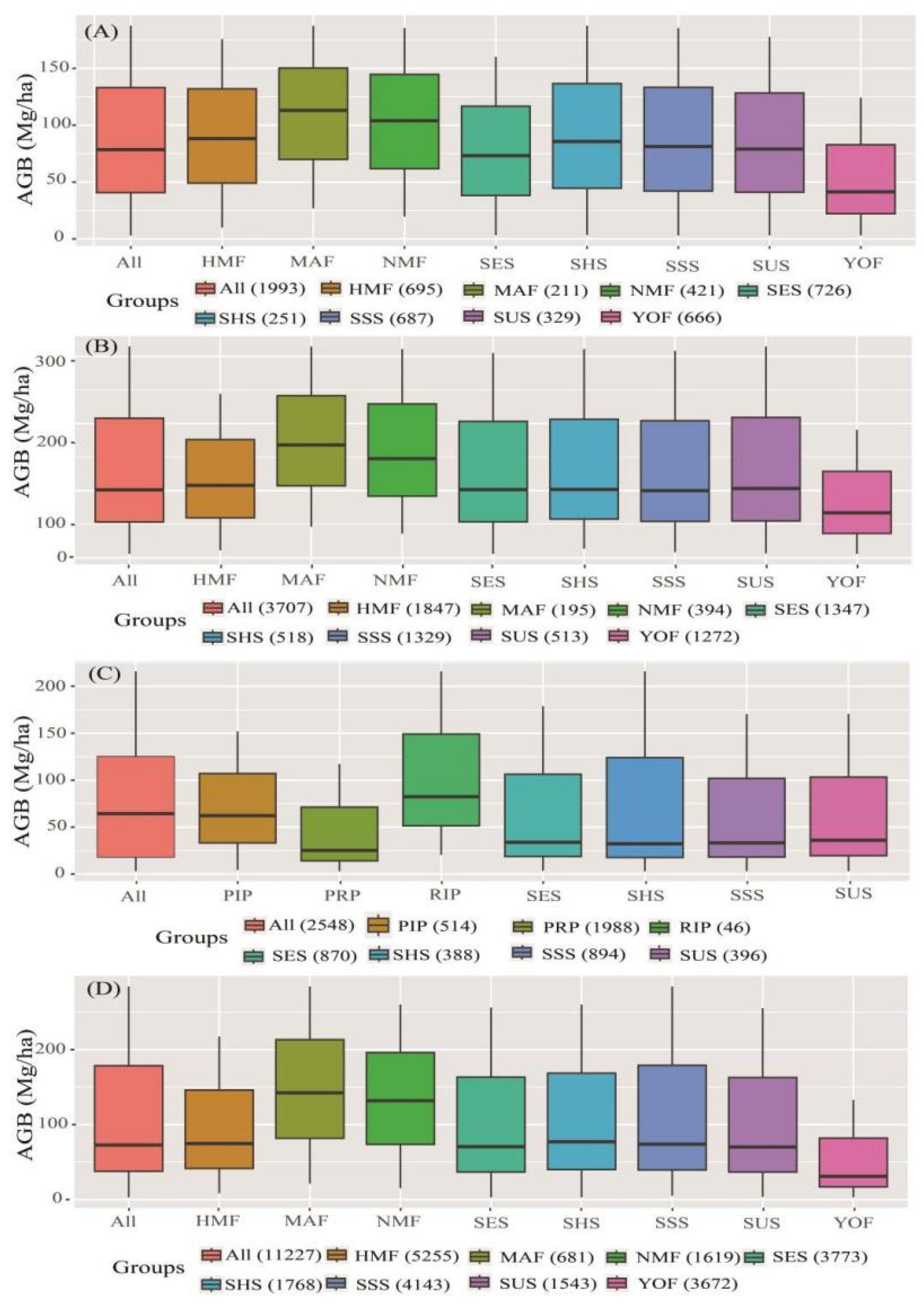
2.3. Forest AGB Data Collection and Processing

The FMI data provide important insights into the spatial distribution patterns of dominant species, notably P. kesiya var. langbianensis and H. brasiliensis, as well as collective species groups such as oak and other broadleaf trees. The AGB of the four forest types was then calculated using the biomass conversion variables method [41]. All the conversion parameters of four forest types are listed in Table 1 [41]. The calculation formula for this method is as follows:
B = V × S V D × B E F
where B is the per unit area of AGB in the sub-compartment (Mg/ha), V is the volume of storage per unit area in the sub-compartment (m3/ha), SVD is the basic wood density (Mg/m3), and BEF is the biomass conversion factor (dimensionless).
Before the estimation models were generated, the sub-compartments were screened, with the outliers identified and filtered based on a threshold of three standard deviations above and below the mean to enhance the reliability of the dataset. Finally, the sub-compartments of the P. kesiya var. langbianensis forests (1993), oak forests (3707), H. brasiliensis forests (2548), and other broadleaf forests (11,227) were utilized to estimate the forest AGB. The statistical parameters of the sub-compartment datasets for the four species or species groups are shown in Figure 3.

2.4. Remote Sensing Data and Variables

2.4.1. Data Accessing and Processing

The digital elevation model (DEM) data were downloaded from the Geospatial Data Cloud website (http://www.gscloud.cn/ (accessed on 1 November 2022)), and processed by georeferencing to match the distribution of the forests. The L8 imagery was also downloaded from the Geospatial Data Cloud website and then preprocessed with radiometric calibration, FLAASH atmospheric correction, and topography correction steps using ENVI 5.3 software [42,43]. Finally, both the DEM and L8 images were resampled to 10 m to ensure consistent image resolution between datasets (Figure 2).
Sentinel 2A is a multispectral instrument with 13 spectral bands spanning the visible to shortwave infrared range, providing imagery with high spatial resolutions of 10–20 m [44]. The S2 Level-1C imagery was downloaded from the Copernicus Open Access Hub (https://scihub.copernicus.eu/dhus/#/home (accessed on 15 November 2022)); this product was selected as there are no Level-2A data before May 2017 available in the study area. The Level-1C data are orthorectified products that represent the reflectance at the top of the atmosphere. These images can then be processed to yield equivalent data to Level-2A products by applying atmospheric correction techniques. The Sen2Cor (version 02.05) plugin in the SNAP toolbox (http://step.esa.int/main/download/snap-download/ (accessed on 15 November 2022)) was used to create L2A products. All the spectral bands were resampled to a 10 m resolution in SNAP. Subsequently, band fusion, radiometric correction, atmospheric correction, topographic correction, cropping, and image splicing [43] were performed in ENVI 5.3 (Figure 2).
To enhance image quality and thereby improve the AGB estimation accuracy, all the images used were chosen to coincide with the period represented by the FMI data. The images with the least cloud cover were chosen to minimize the impact of cloud interference. The details of the images that met these conditions are listed in Table 2.

2.4.2. Extracting Remote Sensing Variables

Original spectral bands, vegetation indices, and image transformations have been widely used to estimate forest AGB [45,46]. Texture measures are also considered one of the main factors that can improve AGB estimation accuracy and better reflect complex or heterogeneous forest structures [19,47]. Therefore, the original spectral bands, vegetation indices, image transformations, and texture measures were extracted from the L8 and S2 images, and the elevation was extracted from the DEM. As shown in Table 3, a comprehensive set of features was extracted from the L8 imagery, encompassing five original spectral bands, 20 vegetation indices, and three image transformations, in addition to 168 texture metrics. These texture metrics were derived from the grey-level co-occurrence matrix (GLCM), capturing various aspects of the texture including the mean (ME), variance (VA), homogeneity (HO), contrast (CN), dissimilarity (Di), entropy (EN), second moment (SM), and correlation (CO). The analysis was conducted using moving window sizes of 3 × 3, 5 × 5, and 7 × 7 pixels to provide a detailed understanding of the spatial characteristics of the imagery. A total of 298 variables, including 11 original bands, 20 vegetation indices, three image transformations, and 264 texture measure variables, were derived from the S2 imagery.

2.4.3. Variable Screening

Variable selection refers to selecting the smallest and most effective subset of variables from the original set to reduce the dimensionality of the variables [21]. Variable selection plays a key role in fitting forest AGB models as it directly affects the performance, interpretability, and applicability of the models [51]. In this study, the correlations between all the variables and the forest AGB were calculated, and only the variables with a significance level of 0.01 on the forest AGB were selected for further analysis. Subsequently, the VIF was employed to screen the chosen variables and examine issues including potential instability in model parameter estimates, reduced explanatory capacity, and poor statistical reliability [52]. Finally, the variables with a significance level of 0.01 and VIF < 10 were selected to estimate the forest AGB.

2.5. Model Fitting

The RF approach is a widely used ensemble machine learning technique that excels in addressing both classification and regression challenges. This technique achieves excellent precision in AGB estimation, has strong robustness against overfitting, and can effectively handle missing data and outliers [53]. The RF model generates new datasets by bootstrapping from the original sample datasets, selecting approximately two-thirds of the data for each bootstrap sample while treating the remaining one-third as out-of-bag (OOB) data [54]. In this study, the RF model was constructed using the randomForest package in R4.3.3 software. To optimize the model’s performance further, we employed a grid search technique, which is a robust method for hyperparameter tuning. This approach systematically searches for each optimal combination of ntree and mtry within a predefined grid according to the different datasets [55]. Specifically, we used a five-fold cross-validation strategy through the CARET package, which allowed the model’s best parameter combination to be adjusted and chosen based on different variables and datasets (https://topepo.github.io/caret/ (accessed on 30 March 2024)) [56]. Finally, 80% of the sub-compartments were used for modeling, while the remaining 20% were used for validation.

2.6. Assessment and Validation of the Models

Model evaluation and validation play a vital role in assessing the accuracy and credibility of the RF model. In this study, the coefficient of determination (R2) and relative root mean square error (rRMSE) were used to evaluate and validate the RF model. The rRMSE metric is a normalized measure of the differences between values predicted by a model and the true values, expressed as a percentage of the observed values. Generally, higher R2 and lower rRMSE values indicate better model performance. These metrics can be calculated as follows:
R 2 = 1 i = 1 n ( y i y ^ i ) 2 i = 1 n ( y i y ¯ i ) 2
r R M S E = i = 1 n y ^ i y i 2 n y ^ i × 100 %
where n is the number of sample observations, i is the ith sample observation, y i is the actual value, y ^ i is the estimated value, and y ¯ i is the mean of the observed samples.

3. Results

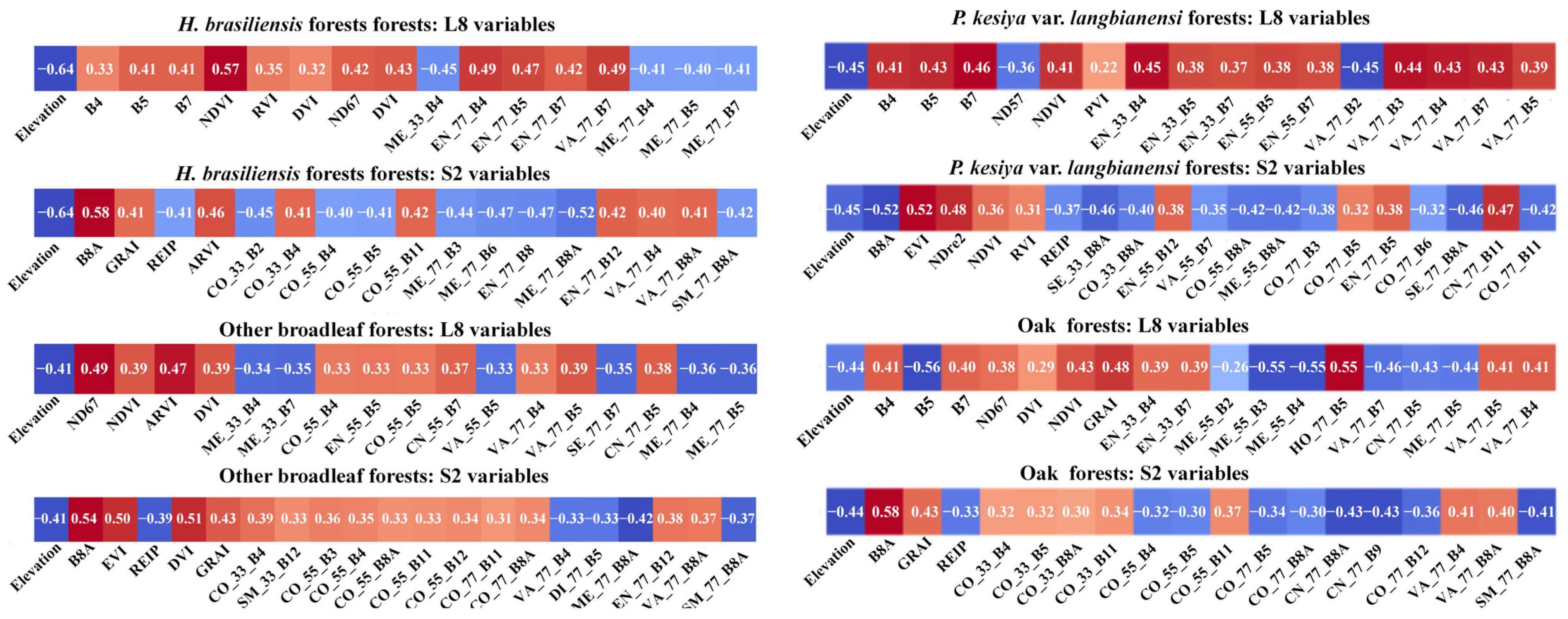
3.1. The Selected Variables for Forest AGB Estimation

As shown in Figure 4, the variables were selected with a significance level of 0.01. Then, the variables selected to estimate the forest AGB also had a VIF < 10 (Table 4). This selection process highlighted the main differences among the variables across the analyzed forest types. The results showed that elevation was sensitive to AGB in all four forest types. At the same time, the selected vegetation index or single bands—most of them are B5 (NIR) and B7 (SWIR2) of the L8 image, B8A (NIR) of the S2 image—that were calculated by the single bands above in both single images and combined images, indicated that in this study area, B5 (NIR), B7 (SWIR2) of L8 and B8A (NIR) of S2 images were more sensitive to forest AGB compared with the other bands. In addition, according to the selected texture measures, the window size of 7 × 7 pixels showed the strongest sensitivity to AGB for four forest types, followed by 5 × 5 pixels; 3 × 3 pixels are the weakest.

3.2. P. kesiya var. langbianensis Forest Models

The results shown in Figure 5 indicate that when using L8, the stratified RF models for P. kesiya var. langbianensis exhibited better model-fitting performance compared to the unstratified models. The unstratified RF model exhibited an R2 value of 0.7036 and an rRMSE of 14.5418 Mg/ha. Among the aspect stratification models, the SHS model achieved the highest R2 value of 0.8214, along with an rRMSE of 9.7722 Mg/ha. Within the age stratification models, the MAF model achieved the best performance, with an R2 value of 0.7928 and an rRMSE of 0.6443 Mg/ha.
Similarly, the stratified models for S2 achieved better performance than the unstratified models. The unstratified RF model achieved an R2 value of 0.7470 and an rRMSE of 14.0112 Mg/ha (Figure 6). In terms of aspect stratification, the SHS model was found to be the most effective, with an R2 value of 0.8305 and an rRMSE of 13.0740 Mg/ha. Within the age stratification models, the HMF model had the best accuracy, with the highest R2 value of 0.8229 and an rRMSE of 9.5232 Mg/ha.
Furthermore, the findings also highlighted that the stratified models integrating L8 and S2 imagery (Figure 7) outperform the unstratified models. The unstratified model registered an R2 of 0.8040 with an rRMSE of 17.2450 Mg/ha. Among the aspect stratification models based on combined L8 + S2 imagery, SHS achieved the best performance, achieving an R2 of value 0.8657 and an rRMSE of 12.0676 Mg/ha. Among the age stratification models, the NEF model recorded the highest R2 value of 0.8233, with an rRMSE of 6.0436 Mg/ha. These results demonstrate the enhanced forest AGB estimation accuracy achieved by the combination of L8 and S2 data. When used individually, the S2 images outperformed the L8 images; however, combining these two datasets achieved the best overall performance.

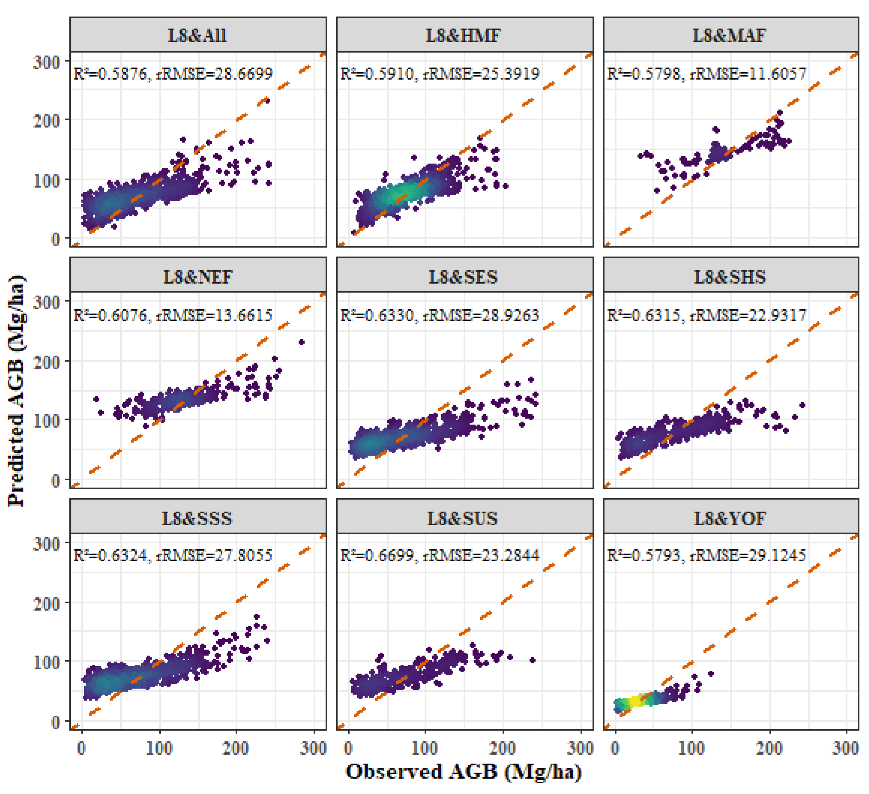
3.3. Oak Forest Models

The stratified models demonstrated superior fitting performance over unstratified models across all oak forest groups, as evidenced from Figure 8, Figure 9 and Figure 10. Among the aspect models using L8 imagery, the SUS model achieved the highest model accuracy with an R2 value of 0.8204 and an rRMSE of 14.7955 Mg/ha. When using S2 imagery, the accuracy of the SUS model further improved, with an R2 value of 0.8365 and an rRMSE of 10.9419 Mg/ha. Within the age stratification models using combined L8 + S2 imagery, the NEF model achieved the best performance in oak forest AGB estimation, with an R2 value of 0.8320 and an rRMSE of 7.8496 Mg/ha. Consequently, the integration of L8 and S2 imagery emerged as the most effective approach for forest AGB estimation in this study.

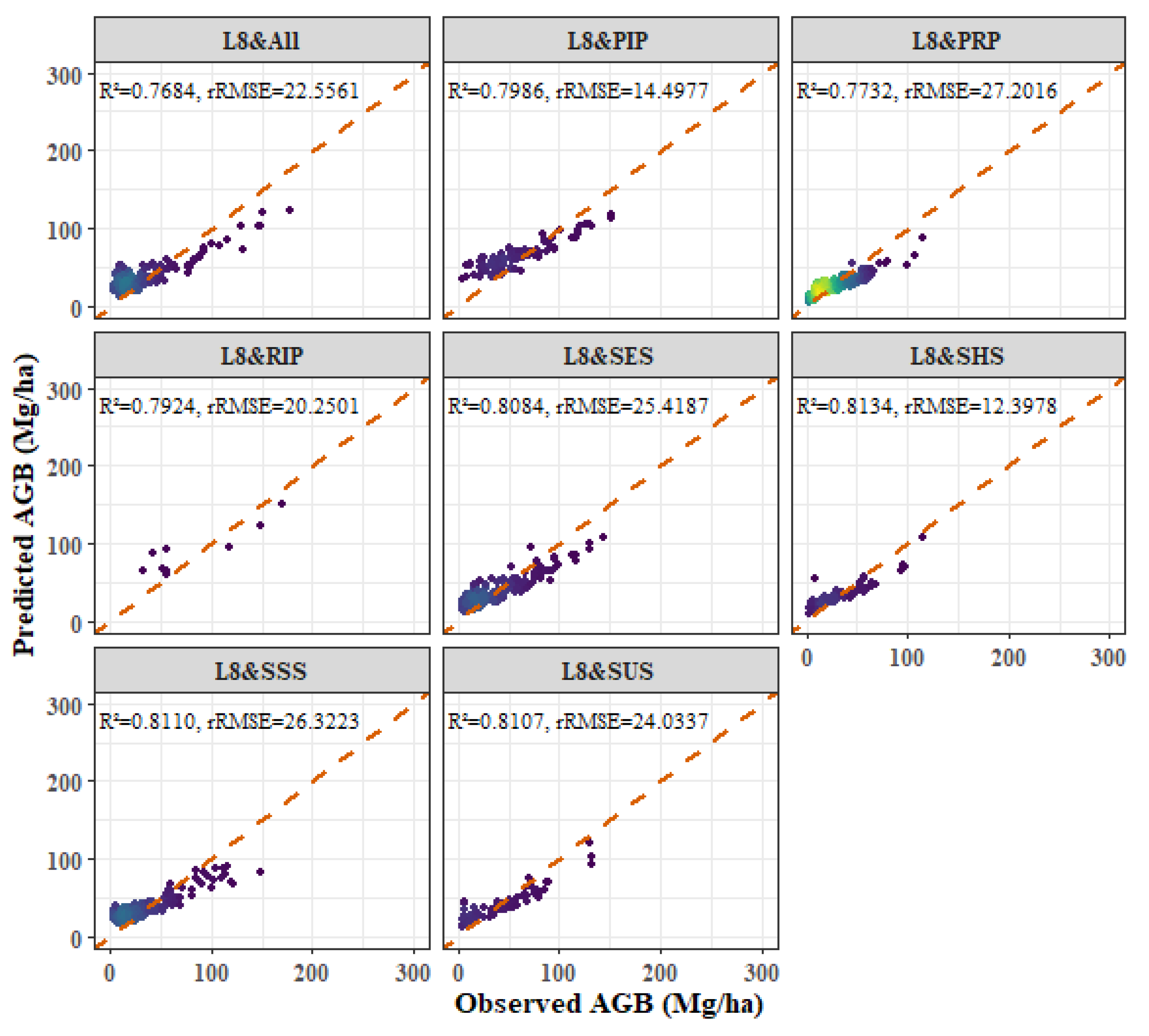
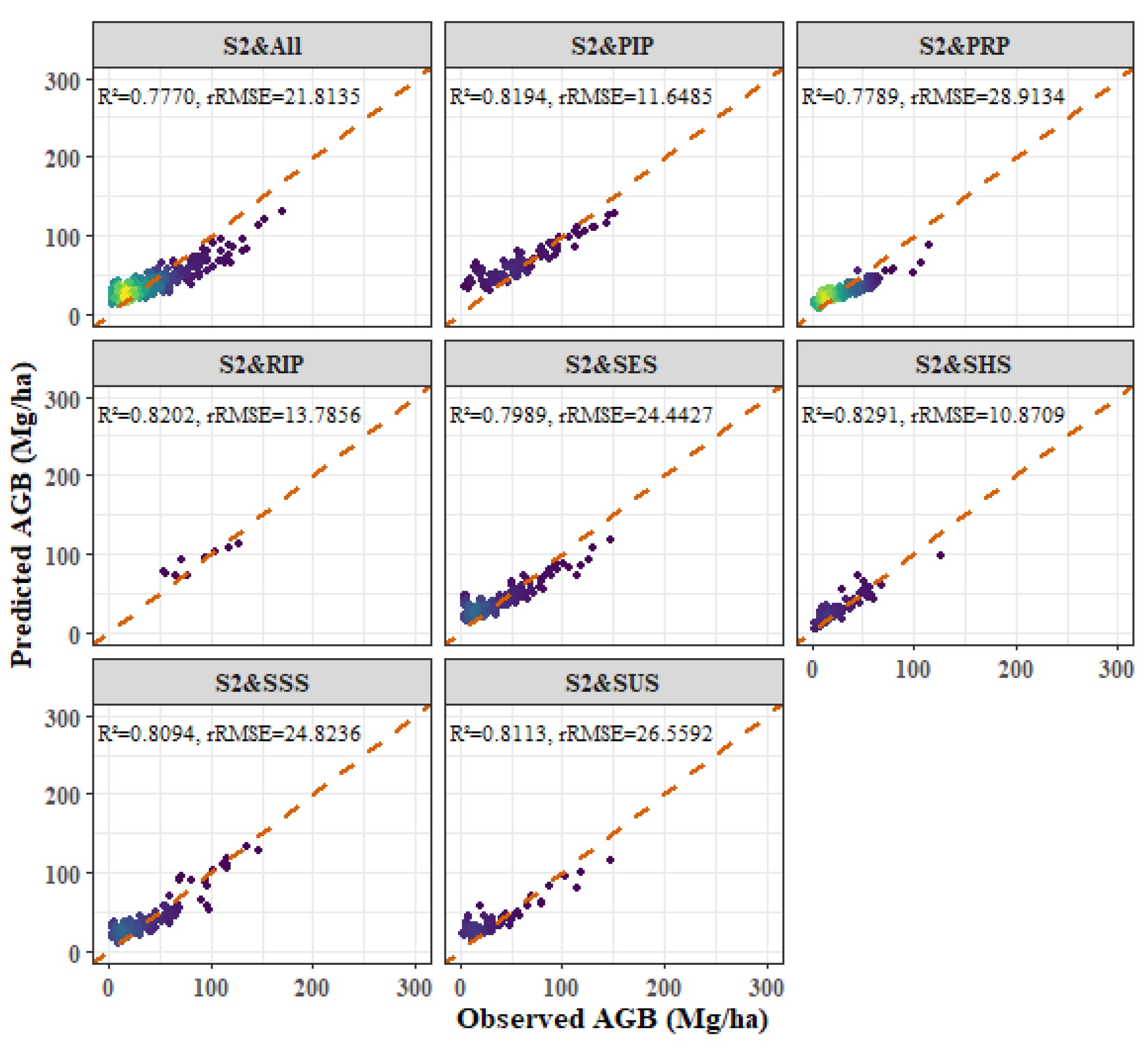
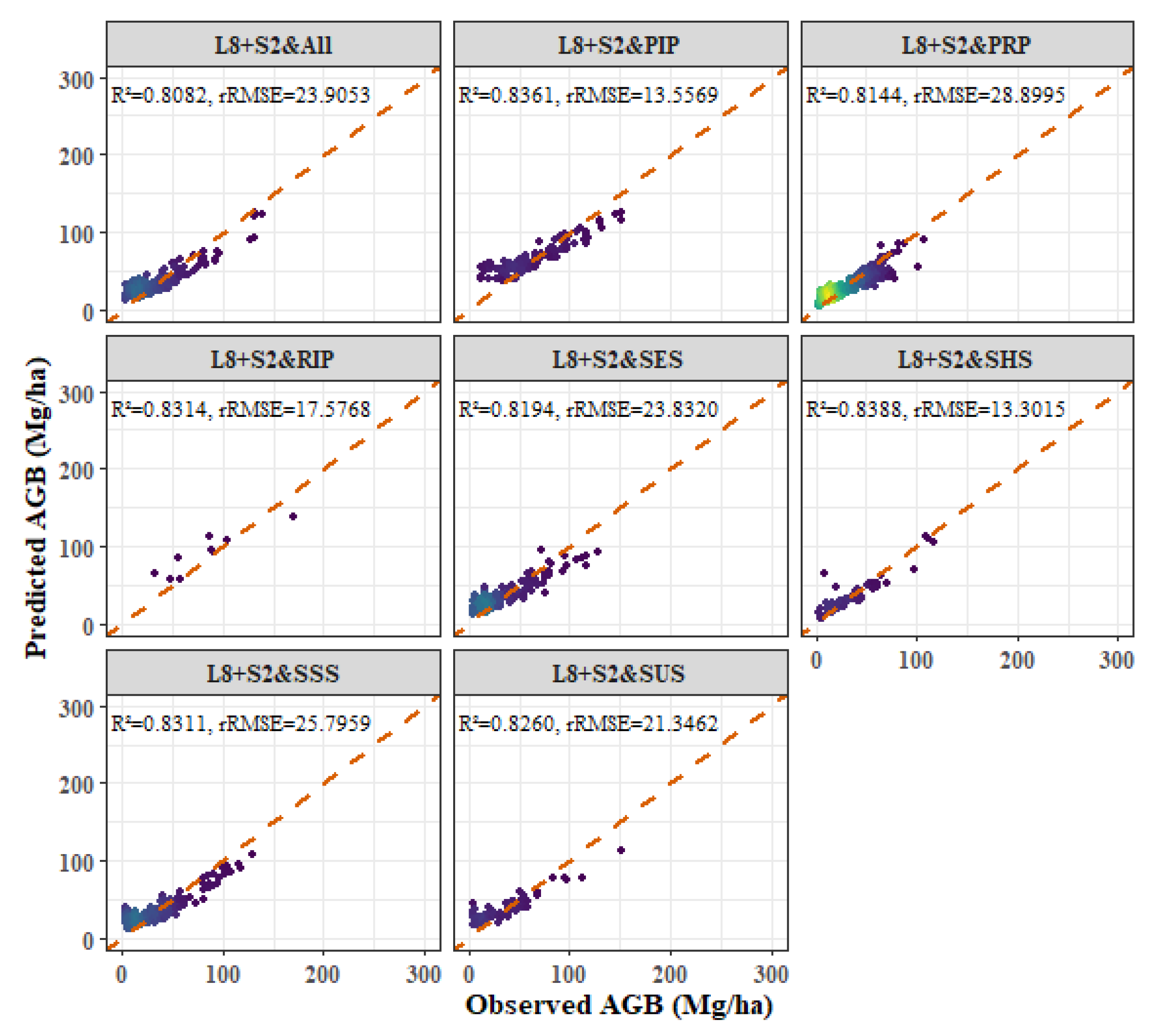
3.4. H. brasiliensis Forest Models

Figure 11, Figure 12 and Figure 13 reveal that stratified models outperform their unstratified counterparts, with the L8 + S2 combination achieving optimal model fitting for H. brasiliensis forest AGB estimation. Among the tested models, the SHS model achieves superior performance using L8 + S2 imagery and consistently outperforms the SUS models, while the SSS models demonstrated improved performance over the SES models.

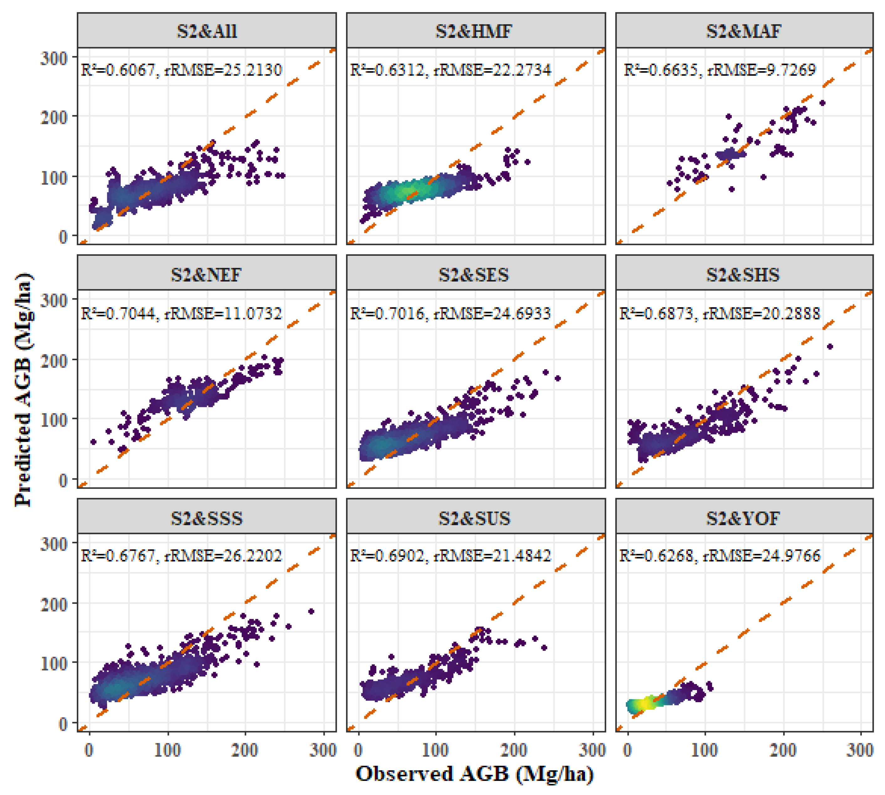
3.5. Other Broadleaf Forest Models

Figure 14, Figure 15 and Figure 16 demonstrate that, among the other broadleaf forest models, the stratified approaches generally outperformed the unstratified ones. The SUS model, utilizing L8 + S2 imagery, achieved the highest accuracy with an R2 value of 0.8240 and an rRMSE of 19.3026 Mg/ha. In contrast, the lowest accuracy was observed in unstratified models using L8 images, with an R2 value of 0.5876 and an rRMSE of 28.6699 Mg/ha. All the aspect stratification models yielded comparable accuracy in forest AGB estimation across similar image sets, while the NEF models achieved the best performance in the age stratification analysis.

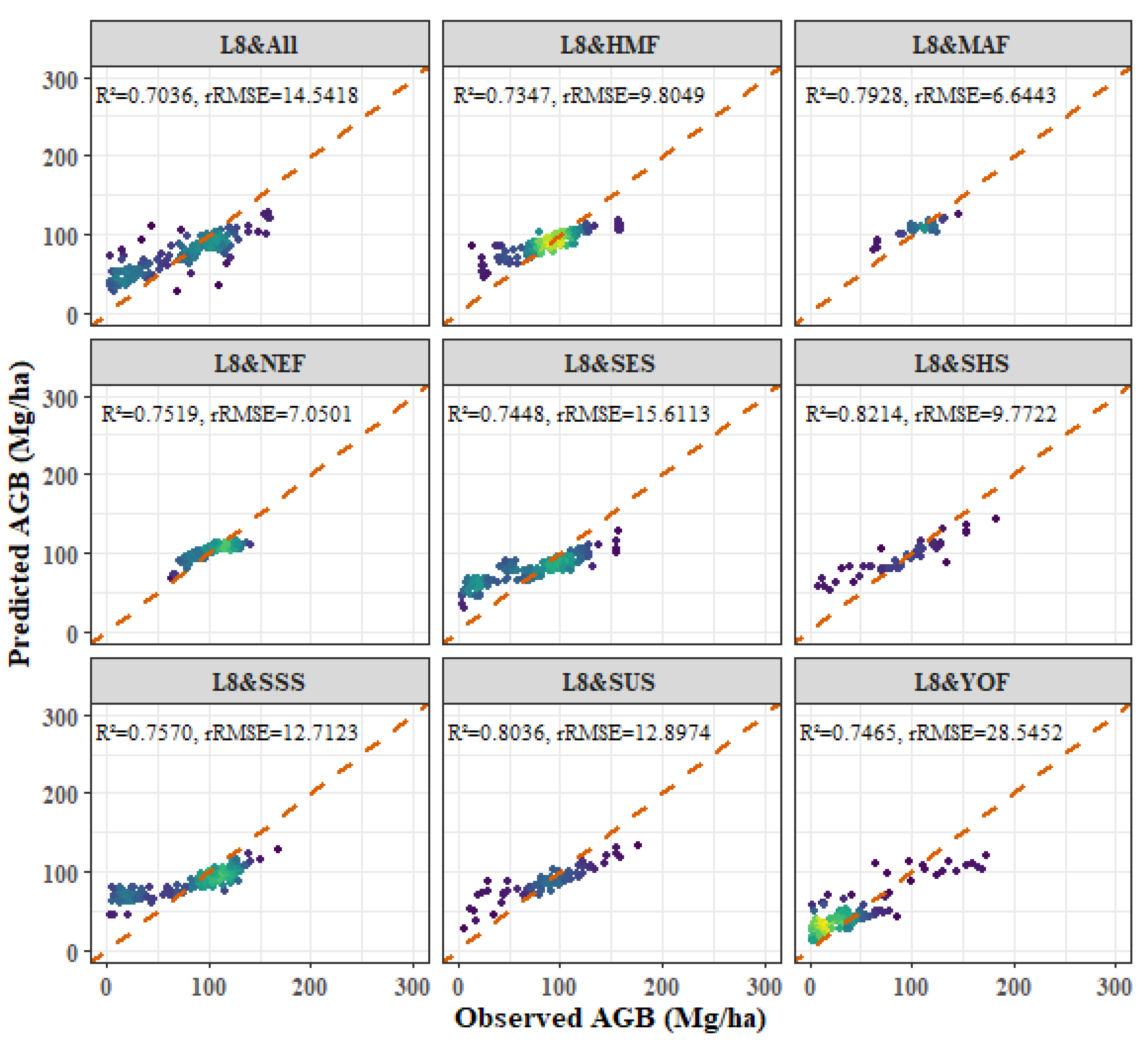
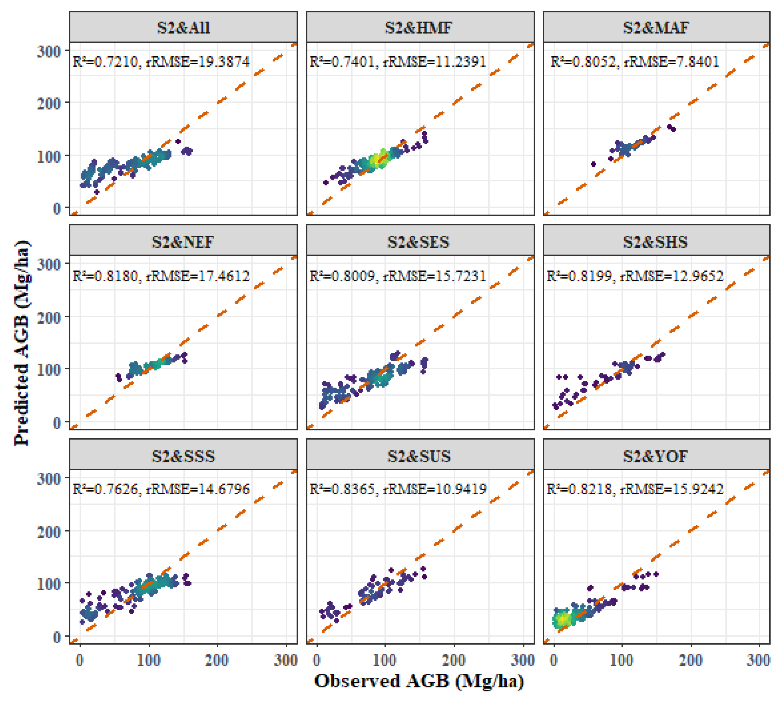
3.6. Models Comparison

The analysis across stratified and unstratified models in this investigation highlights the effectiveness of age and aspect stratifications in enhancing model precision beyond that achieved by the unstratified models. The age stratification analysis revealed that the NEF models achieved markedly improved accuracy across all forest types relative to the unstratified models, with other models within this stratification showing similar levels of accuracy. In aspect stratification, the accuracy in the P. kesiya var. langbianensis and H. brasiliensis forests was notably higher in the SHS models than in SUS models, whereas oak and other broadleaf forests demonstrated greater accuracy in SUS models compared to SHS models. In descending order of accuracy, the hierarchy of forest types was as follows: P. kesiya var. langbianensis forests > H. brasiliensis forests > oak forests > other broadleaf forests. Furthermore, an analysis of the scatter plots revealed consistent patterns of both overestimation and underestimation among the models, with each model exhibiting distinct biases that varied in magnitude across different data ranges.

4. Discussion

4.1. Variables Affecting Forest AGB

The analysis of the four forest types revealed marked differences in the impacts of variables on forest AGB, thus emphasizing the critical role played by variable selection in refining forest AGB estimation models for improved interpretability and optimal usage of remote sensing data utility [57]. The variables with a significance level below 0.01 and a VIF under 10 were selected to maximize their fit with forest AGB and improve estimation accuracy. Furthermore, the comparison between different imagery configurations—L8 + S2 outperforming S2, which in turn surpassed S8—demonstrates the benefit of integrating L8 and S2 datasets. This data integration not only improves AGB estimation accuracy but also emphasizes the additional insights gained from S2, particularly through its red-edge bands, which provide important constraints for vegetation monitoring insights [58].
The hierarchy of selected variables (in which texture measures outperform the vegetation indices and original bands) highlights the important role of texture measures in delineating complex surface features and spatial dynamics in AGB estimation [50,59]. Conversely, image transformation variables were consistently excluded across all forest types and sensors, likely due to their generalized variance focus and failure to constrain specific or non-linear biomass correlations, including those involving texture indices [60]. Elevation was found to be a key factor controlling forest AGB, as changes in elevation affect variations in temperature, precipitation, and soil properties. For instance, at higher elevations, there are typically lower temperatures, worse soil nutrition, and more uneven precipitation, which collectively shape the dynamics and distribution of vegetation in lowland tropical forests [61].
In addition, bands B5 (NIR) and B7 (SWIR2) of L8, along with B8A (NIR) of S2, were found to be more strongly correlated with forest AGB, indicating their greater sensitivity to vegetation health and biomass estimation [62]. These bands, especially NIR, are essential for gauging vegetation structure, chlorophyll content, soil moisture, and biomass, and thus form an important part of AGB estimation [63]. Furthermore, the superior performance of 7 × 7 pixel windows in AGB estimation over smaller sizes can be attributed to the ability of larger window sizes to capture more spatial information, mitigate noise, and offer improved contextual insights [64].

4.2. Stratified and Unstratified RF Models

This investigation found that stratified models significantly outperform unstratified models in the context of AGB estimation, with R2 values ranging from 0.5876 to 0.8675. For comparison, Phua et al. [65] applied airborne LiDAR to AGB estimation for a logged-over Malaysian lowland rainforest, highlighting a notable improvement in model accuracy, represented by an increase in R2 values from 0.2700 to 0.6700. A similar study reported a significant correlation in tropical forest AGB estimates using L- and C-band data, with R2 values ranging from 0.6900 to 0.7700 [66]. However, these studies achieved a lower forest AGB estimation accuracy than the present work, highlighting the benefits of the stratified model approach used in this study. The estimation accuracy of P. densata forest AGB in Yunnan of Southwestern China was improved by incorporating the stand age as a dummy variable in models [26]. The findings of the present study show that the integration of age and aspect stratification can enhance the AGB estimation accuracy in lowland tropical forests; these findings are consistent with previous findings that vegetation type and aspect stratification can be used to improve AGB estimation [27].
Furthermore, the NEF models achieved the best performance among the age stratification models. Higher forest heterogeneity may result in lower accuracy [3], and the NEF and MAF forests have notably higher forest heterogeneity and more complex vertical structures than the YOF and HMF forests. However, AGB underestimation may occur in MAF forests due to the generally higher AGB values in these areas [67], while lower forest heterogeneity can improve the estimation accuracy [26,68]. The higher accuracy of the NEF stratification model compared to the YOF and HMF stratification models may relate to the greater vertical structure variability, wider biomass range, greater diversity of growth stages, and increased availability of data in near-mature forests; overestimation also often occurs in areas with smaller AGB values [69]. Therefore, the NEF model showed the largest improvement among the AGB estimation models.
Furthermore, the differences in peak accuracy between the aspect stratification models across the four forest types can be attributed to the biological differences between species, with P. kesiya var. langbianensis and H. brasiliensis classified as intolerant plants, and the majority of oak and other broadleaf species identified as shade-tolerant plants [38]. This difference suggests that masculine species grow better in sunlit aspects, benefiting from and contributing to greater forest heterogeneity, in contrast to feminine species, which exhibit reduced heterogeneity in sunny aspects relative to shaded aspects [70]. Across the four forest types, the best AGB estimation accuracy was achieved in P. kesiya var. langbianensis forests, followed by H. brasiliensis, oak, and then other broadleaf forests. This pattern may relate to the inherent differences between coniferous and broad-leaved forests, with improved estimation accuracy achieved in the former type, as demonstrated by the estimates for P. kesiya var. langbianensis [27]. The H. brasiliensis forests, primarily cultivated in Xishuangbanna, contrast with the predominantly natural oak and other broadleaf forests; thus, higher accuracy was achieved for AGB estimation in planted forests, likely due to their reduced heterogeneity compared to natural forests [38]. Additionally, the other broadleaf forests showed differences in their spectral reflection characteristics due to the complex mixed species in these areas, leading to greater spectral heterogeneity and reduced AGB estimation accuracy. Although the inclusion of different stratification factors improved the estimation accuracy in other broadleaf forests, the estimates still showed lower accuracy than those in other forest types [38].
In addition, AGB overestimation or underestimation also commonly occurs due to the presence of a complex canopy structure, and high AGB values may cause the reflectance saturation phenomenon to occur, leading to value underestimation. Conversely, the low canopy density in young forests may cause the reflection values to be affected by understory vegetation such as shrubs, grasses, and bare land, thus resulting in an overestimation of the low biomass value of these forests [67,71]. These discrepancies in estimation were identified as some of the main sources of error in forest AGB assessment [72]. However, implementing stratified models has been shown to help mitigate these biases, thus improving the estimation accuracy beyond that achievable with unstratified models. Overall, this finding emphasizes the importance of using stratified variable approaches to achieve higher forest AGB estimation accuracy.

4.3. Limitations and Future Research

In this study, we used stratified and unstratified models to estimate the AGB of four types of tropical lowland forests in Xishuangbanna using L8 and S2 images. While both the L8 and S2 were optical sensors, other remote sensing data, such as SPOT, MODIS, Sentinel 1A, etc., are also commonly used in forest AGB estimation. Thus, it is important to explore the effects of stratified models in other remote sensing sources. Additionally, although the stratified models can reduce the effects of overestimation or underestimation, the uncertainty caused by these factors was still a challenge and increased the error in our models. We intend to explore other methods or models that could be used to reduce this uncertainty and further improve the estimation accuracy. In addition, we only adopted the dominant tree species of lowland tropical forests in Xishuangbanna as a case study: in the future, we intend to apply this approach to other lowland tropical forests globally to verify the applicability of the stratified models and compare inter-regional variations in the characteristics of lowland tropical forests.

5. Conclusions

To enhance the precision of AGB estimation in lowland tropical forests, this study focuses on refining the estimation capabilities of stratified models. We conducted a comprehensive evaluation of AGB in diverse lowland tropical forest types, including P. kesiya var. langbianensis, oak, H. brasiliensis, and other broadleaf forests. This assessment was performed with both stratified and unstratified RF models, using data from L8 and S2 imagery. The main results of this study are as follows:
(1)
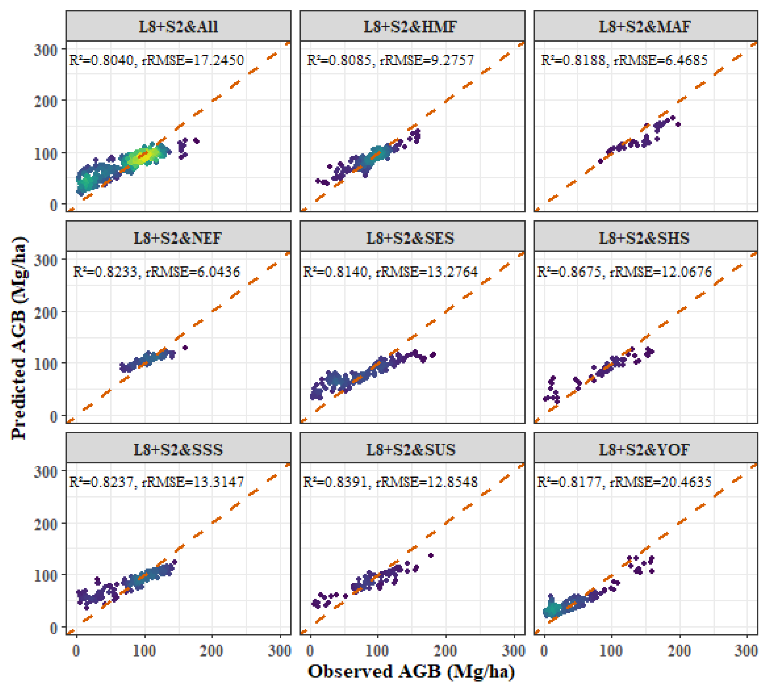
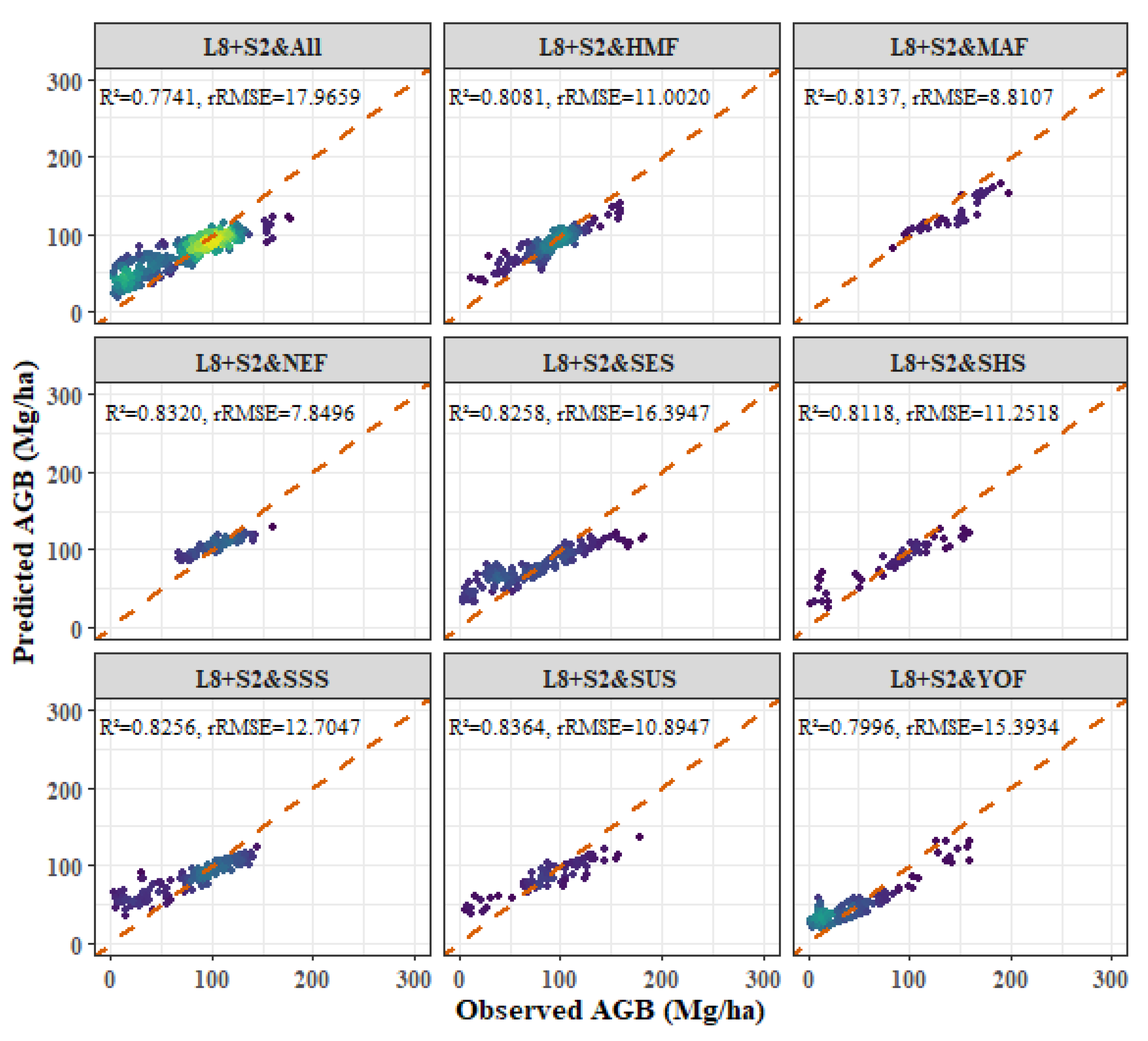
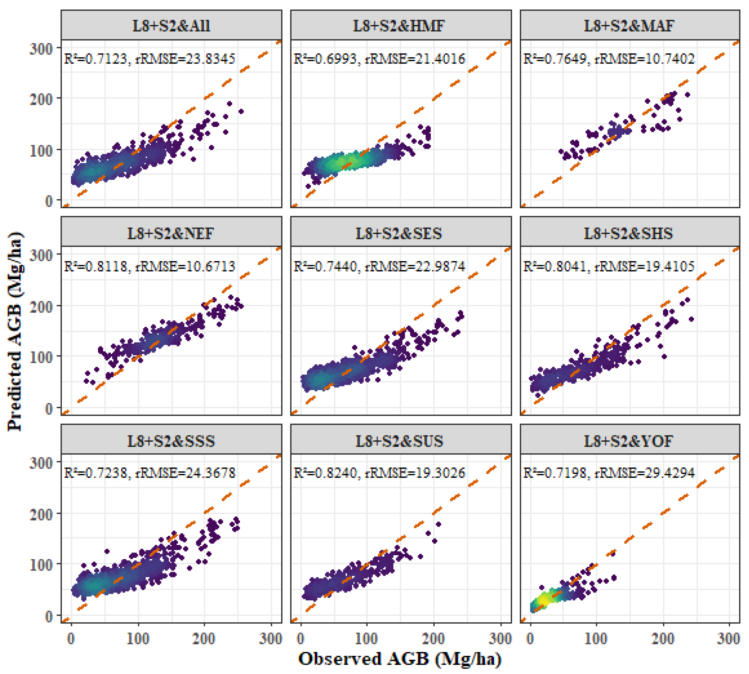
Among the four forest types, the fitting effect of L8 and S2 combined images is better than that of S2 or L8 alone. The R2 values for the combined L8 + S2 analysis for the four forest types were as follows: P. kesiya var. langbianensis (0.8040), oak (0.7741), H. brasiliensis (0.8082), and other broadleaf forests (0.7123).
(2)
Age and aspect stratification significantly improved the estimation accuracy of AGB, and the accuracy of the NEF age stratification model was significantly improved. The improvements in R2 values were as follows: P. kesiya var. langbianensis (0.02), oak (0.06), H. brasiliensis (0.03), and other broadleaf forests (0.10). In aspect stratification, the SHS model had the best fitting effect for P. kesiya var. langbianensis (0.8675) and H. brasiliensis (0.8388), while the SUS model achieved the best fitting effect on the AGB model of oak (0.8364) and other broad-leaved trees (0.8240).
Overall, our study highlights the validity of using multi-source remote sensing data for the accurate estimation of AGB in lowland tropical forests and the critical role played by stratification in such assessments. This approach has important applications in carbon accounting and forest management, both in Xishuangbanna and in similar ecosystems worldwide.

Author Contributions

Y.W. participated in the collection of the data, conducted the data analysis, and wrote the draft of the paper; T.L., T.H., X.Z., Z.L., Z.Y., B.G., E.W., Z.F., H.L. and C.L. helped with the data analysis, and part of the graphs; L.W. and W.X. gave some suggestions and guidance; G.O. supervised and coordinated the research project, designed the experiment, and revised the paper. All authors have read and agreed to the published version of the manuscript.

Funding

This research was jointly supported by the Scientific Research Fund Project of Yunnan Provincial Education Department (2023Y0732), and the Education Talent of Xingdian Talent Support Program of Yunnan Province, China.

Data Availability Statement

Data is contained within the article.

Acknowledgments

We would like to acknowledge all the people who have contributed to this paper.

Conflicts of Interest

The authors declare no conflicts of interest.

References

  1. Lulandala, L.; Bargués-Tobella, A.; Masao, C.A.; Nyberg, G.; Ilstedt, U. The size of clearings for charcoal production in miombo woodlands affects soil hydrological properties and soil organic carbon. For. Ecol. Manag. 2023, 529, 120701. [Google Scholar] [CrossRef]
  2. Poorter, L.; van der Sande, M.T.; Thompson, J.; Arets, E.J.; Alarcón, A.; Álvarez-Sánchez, J.; Ascarrunz, N.; Balvanera, P.; Barajas-Guzmán, G.; Boit, A. Diversity enhances carbon storage in tropical forests. Glob. Ecol. Biogeogr. 2015, 24, 1314–1328. [Google Scholar] [CrossRef]
  3. Lu, D.; Chen, Q.; Wang, G.; Liu, L.; Li, G.; Moran, E. A survey of remote sensing-based aboveground biomass estimation methods in forest ecosystems. Int. J. Digit. Earth 2016, 9, 63–105. [Google Scholar] [CrossRef]
  4. Ou, G.; Lv, Y.; Xu, H.; Wang, G. Improving forest aboveground biomass estimation of Pinus densata forest in Yunnan of Southwest China by spatial regression using Landsat 8 images. Remote Sens. 2019, 11, 2750. [Google Scholar] [CrossRef]
  5. Tang, J.; Liu, Y.; Li, L.; Liu, Y.; Wu, Y.; Xu, H.; Ou, G. Enhancing aboveground biomass estimation for three pinus forests in yunnan, SW China, using landsat 8. Remote Sens. 2022, 14, 4589. [Google Scholar] [CrossRef]
  6. Vafaei, S.; Soosani, J.; Adeli, K.; Fadaei, H.; Naghavi, H.; Pham, T.D.; Tien Bui, D. Improving accuracy estimation of Forest Aboveground Biomass based on incorporation of ALOS-2 PALSAR-2 and Sentinel-2A imagery and machine learning: A case study of the Hyrcanian forest area (Iran). Remote Sens. 2018, 10, 172. [Google Scholar] [CrossRef]
  7. Mansaray, L.R.; Wang, F.; Huang, J.; Yang, L.; Kanu, A.S. Accuracies of support vector machine and random forest in rice mapping with Sentinel-1A, Landsat-8 and Sentinel-2A datasets. Geocarto Int. 2020, 35, 1088–1108. [Google Scholar] [CrossRef]
  8. Imran, A.; Ahmed, S. Potential of Landsat-8 spectral indices to estimate forest biomass. Int. J. Hum. Cap. Urban Manag. 2018, 3, 303. [Google Scholar]
  9. Li, C.; Li, Y.; Li, M. Improving forest aboveground biomass (AGB) estimation by incorporating crown density and using landsat 8 OLI images of a subtropical forest in Western Hunan in Central China. Forests 2019, 10, 104. [Google Scholar] [CrossRef]
  10. Bousbaa, M.; Htitiou, A.; Boudhar, A.; Eljabiri, Y.; Elyoussfi, H.; Bouamri, H.; Ouatiki, H.; Chehbouni, A. High-resolution monitoring of the snow cover on the Moroccan Atlas through the spatio-temporal fusion of Landsat and Sentinel-2 images. Remote Sens. 2022, 14, 5814. [Google Scholar] [CrossRef]
  11. Pandit, S.; Tsuyuki, S.; Dube, T. Estimating above-ground biomass in sub-tropical buffer zone community forests, Nepal, using Sentinel 2 data. Remote Sens. 2018, 10, 601. [Google Scholar] [CrossRef]
  12. Coops, N.C.; Tompalski, P.; Goodbody, T.R.; Achim, A.; Mulverhill, C. Framework for near real-time forest inventory using multi source remote sensing data. Forestry 2023, 96, 1–19. [Google Scholar] [CrossRef]
  13. Zhao, X.; Yu, B.; Liu, Y.; Chen, Z.; Li, Q.; Wang, C.; Wu, J. Estimation of poverty using random forest regression with multi-source data: A case study in Bangladesh. Remote Sens. 2019, 11, 375. [Google Scholar] [CrossRef]
  14. Huang, H.; Liu, C.; Wang, X.; Zhou, X.; Gong, P. Integration of multi-resource remotely sensed data and allometric models for forest aboveground biomass estimation in China. Remote Sens. Environ. 2019, 221, 225–234. [Google Scholar] [CrossRef]
  15. Huang, T.; Ou, G.; Wu, Y.; Zhang, X.; Liu, Z.; Xu, H.; Xu, X.; Wang, Z.; Xu, C. Estimating the Aboveground Biomass of Various Forest Types with High Heterogeneity at the Provincial Scale Based on Multi-Source Data. Remote Sens. 2023, 15, 3550. [Google Scholar] [CrossRef]
  16. Sa, R.; Fan, W. Estimation of Forest Parameters in Boreal Artificial Coniferous Forests Using Landsat 8 and Sentinel-2A. Remote Sens. 2023, 15, 3605. [Google Scholar] [CrossRef]
  17. Tian, L.; Wu, X.; Tao, Y.; Li, M.; Qian, C.; Liao, L.; Fu, W. Review of Remote Sensing-Based Methods for Forest Aboveground Biomass Estimation: Progress, Challenges, and Prospects. Forests 2023, 14, 1086. [Google Scholar] [CrossRef]
  18. Chatziantoniou, A.; Petropoulos, G.P.; Psomiadis, E. Co-Orbital Sentinel 1 and 2 for LULC mapping with emphasis on wetlands in a mediterranean setting based on machine learning. Remote Sens. 2017, 9, 1259. [Google Scholar] [CrossRef]
  19. Kuplich, T.; Curran, P.J.; Atkinson, P.M. Relating SAR image texture to the biomass of regenerating tropical forests. Int. J. Remote Sens. 2005, 26, 4829–4854. [Google Scholar] [CrossRef]
  20. Zhang, L.; Shao, Z.; Liu, J.; Cheng, Q. Deep learning based retrieval of forest aboveground biomass from combined LiDAR and landsat 8 data. Remote Sens. 2019, 11, 1459. [Google Scholar] [CrossRef]
  21. Li, Y.; Li, C.; Li, M.; Liu, Z. Influence of variable selection and forest type on forest aboveground biomass estimation using machine learning algorithms. Forests 2019, 10, 1073. [Google Scholar] [CrossRef]
  22. Karlson, M.; Ostwald, M.; Reese, H.; Sanou, J.; Tankoano, B.; Mattsson, E. Mapping tree canopy cover and aboveground biomass in Sudano-Sahelian woodlands using Landsat 8 and random forest. Remote Sens. 2015, 7, 10017–10041. [Google Scholar] [CrossRef]
  23. Purohit, S.; Aggarwal, S.; Patel, N. Estimation of forest aboveground biomass using combination of Landsat 8 and Sentinel-1A data with random forest regression algorithm in Himalayan Foothills. Trop. Ecol. 2021, 62, 288–300. [Google Scholar] [CrossRef]
  24. Zeng, N.; Ren, X.; He, H.; Zhang, L.; Zhao, D.; Ge, R.; Li, P.; Niu, Z. Estimating grassland aboveground biomass on the Tibetan Plateau using a random forest algorithm. Ecol. Indic. 2019, 102, 479–487. [Google Scholar] [CrossRef]
  25. Pan, Y.; Birdsey, R.A.; Phillips, O.L.; Jackson, R.B. The structure, distribution, and biomass of the world’s forests. Annu. Rev. Ecol. Evol. Syst. 2013, 44, 593–622. [Google Scholar] [CrossRef]
  26. Ou, G.; Li, C.; Lv, Y.; Wei, A.; Xiong, H.; Xu, H.; Wang, G. Improving Aboveground Biomass Estimation of Pinus densata Forests in Yunnan Using Landsat 8 Imagery by Incorporating Age Dummy Variable and Method Comparison. Remote Sens. 2019, 11, 738. [Google Scholar] [CrossRef]
  27. Zhao, P.; Lu, D.; Wang, G.; Wu, C.; Huang, Y.; Yu, S. Examining spectral reflectance saturation in Landsat imagery and corresponding solutions to improve forest aboveground biomass estimation. Remote Sens. 2016, 8, 469. [Google Scholar] [CrossRef]
  28. Chen, Y.; Li, L.; Lu, D.; Li, D. Exploring bamboo forest aboveground biomass estimation using Sentinel-2 data. Remote Sens. 2018, 11, 7. [Google Scholar] [CrossRef]
  29. Gentry, A.H. Tropical forest biodiversity: Distributional patterns and their conservational significance. Oikos 1992, 63, 19–28. [Google Scholar] [CrossRef]
  30. Cao, M.; Zou, X.; Warren, M.; Zhu, H. Tropical forests of xishuangbanna, China. Biotropica J. Biol. Conserv. 2006, 38, 306–309. [Google Scholar]
  31. Chen, Y.; Marino, J.; Chen, Y.; Tao, Q.; Sullivan, C.D.; Shi, K.; Macdonald, D.W. Predicting hotspots of human-elephant conflict to inform mitigation strategies in Xishuangbanna, Southwest China. PLoS ONE 2016, 11, e0162035. [Google Scholar] [CrossRef]
  32. Zhu, H.; Cao, M.; Hu, H. Geological history, flora, and vegetation of Xishuangbanna, Southern Yunnan, China. Biotropica J. Biol. Conserv. 2006, 38, 310–317. [Google Scholar]
  33. Mammides, C.; Goodale, E.; Dayananda, S.K.; Kang, L.; Chen, J. Do acoustic indices correlate with bird diversity? Insights from two biodiverse regions in Yunnan Province, south China. Ecol. Indic. 2017, 82, 470–477. [Google Scholar] [CrossRef]
  34. Singh, J.; Rawat, Y.; Chaturvedi, O. Replacement of oak forest with pine in the Himalaya affects the nitrogen cycle. Nature 1984, 311, 54–56. [Google Scholar] [CrossRef]
  35. Liu, W.; Li, J.; Lu, H.; Wang, P.; Luo, Q.; Liu, W.; Li, H. Vertical patterns of soil water acquisition by non-native rubber trees (Hevea brasiliensis) in Xishuangbanna, southwest China. Ecohydrology 2014, 7, 1234–1244. [Google Scholar] [CrossRef]
  36. Li, H.; Ma, Y.; Aide, T.M.; Liu, W. Past, present and future land-use in Xishuangbanna, China and the implications for carbon dynamics. For. Ecol. Manag. 2008, 255, 16–24. [Google Scholar] [CrossRef]
  37. Pregitzer, K.S.; Euskirchen, E.S. Carbon cycling and storage in world forests: Biome patterns related to forest age. Glob. Chang. Biol. 2004, 10, 2052–2077. [Google Scholar] [CrossRef]
  38. Wu, Z.; Zhu, Y. The Vegetation of Yunnan; Science Press: Beijing, China, 1987. [Google Scholar]
  39. Suratman, M.; Bull, G.; Leckie, D.; Lemay, V.; Marshall, P.; Mispan, M. Prediction models for estimating the area, volume, and age of rubber (Hevea brasiliensis) plantations in Malaysia using Landsat TM data. Int. For. Rev. 2004, 6, 1–12. [Google Scholar] [CrossRef]
  40. Jianhui, X. Forest Ecology (Revised Edition); China Forestry Publishing House: Beijing, China, 2006; Volume 92, pp. 61–62. [Google Scholar]
  41. Xu, H.; Zhang, Z.; Ou, G.; Shi, H. A Study on Estimation and Distribution for Forest Biomass and Carbon Storage in Yunnan Province; Yunnan Science and Technology Press: Kunming, China, 2019. [Google Scholar]
  42. Kaufman, Y.J.; Tanre, D. Strategy for direct and indirect methods for correcting the aerosol effect on remote sensing: From AVHRR to EOS-MODIS. Remote Sens. Environ. 1996, 55, 65–79. [Google Scholar] [CrossRef]
  43. Li, L.; Zhou, B.; Liu, Y.; Wu, Y.; Tang, J.; Xu, W.; Wang, L.; Ou, G. Reduction in Uncertainty in Forest Aboveground Biomass Estimation Using Sentinel-2 Images: A Case Study of Pinus densata Forests in Shangri-La City, China. Remote Sens. 2023, 15, 559. [Google Scholar] [CrossRef]
  44. Gascon, F.; Bouzinac, C.; Thépaut, O.; Jung, M.; Francesconi, B.; Louis, J.; Lonjou, V.; Lafrance, B.; Massera, S.; Gaudel-Vacaresse, A. Copernicus Sentinel-2A calibration and products validation status. Remote Sens. 2017, 9, 584. [Google Scholar] [CrossRef]
  45. Huete, A.; Liu, H.; Batchily, K.; Van Leeuwen, W. A comparison of vegetation indices over a global set of TM images for EOS-MODIS. Remote Sens. Environ. 1997, 59, 440–451. [Google Scholar] [CrossRef]
  46. Venancio, L.P.; Mantovani, E.C.; do Amaral, C.H.; Neale, C.M.U.; Gonçalves, I.Z.; Filgueiras, R.; Eugenio, F.C. Potential of using spectral vegetation indices for corn green biomass estimation based on their relationship with the photosynthetic vegetation sub-pixel fraction. Agric. Water Manag. 2020, 236, 106155. [Google Scholar] [CrossRef]
  47. Haralick, R.M.; Shanmugam, K.; Dinstein, I.H. Textural features for image classification. IEEE Trans. Syst. Man Cybern. 1973, SMC-3, 610–621. [Google Scholar] [CrossRef]
  48. Dube, T.; Mutanga, O. Investigating the robustness of the new Landsat-8 Operational Land Imager derived texture metrics in estimating plantation forest aboveground biomass in resource constrained areas. ISPRS J. Photogramm. Remote Sens. 2015, 108, 12–32. [Google Scholar] [CrossRef]
  49. Li, C.; Zhou, L.; Xu, W. Estimating aboveground biomass using Sentinel-2 MSI data and ensemble algorithms for grassland in the Shengjin Lake Wetland, China. Remote Sens. 2021, 13, 1595. [Google Scholar] [CrossRef]
  50. Toutin, T. Elevation modelling from satellite visible and infrared (VIR) data. Int. J. Remote Sens. 2010, 22, 1097–1125. [Google Scholar] [CrossRef]
  51. Li, X.; Liu, Z.; Lin, H.; Wang, G.; Sun, H.; Long, J.; Zhang, M. Estimating the growing stem volume of Chinese pine and larch plantations based on fused optical data using an improved variable screening method and stacking algorithm. Remote Sens. 2020, 12, 871. [Google Scholar] [CrossRef]
  52. Miles, J. Tolerance and variance inflation factor. In Wiley Statsref: Statistics Reference Online; John Wiley & Sons: Hoboken, NJ, USA, 2014. [Google Scholar]
  53. Qi, Y. Random forest for bioinformatics. In Ensemble Machine Learning: Methods and Applications; Springer: Berlin/Heidelberg, Germany, 2012; pp. 307–323. [Google Scholar]
  54. Rigatti, S.J. Random forest. J. Insur. Med. 2017, 47, 31–39. [Google Scholar] [CrossRef]
  55. Shekar, B.; Dagnew, G. Grid search-based hyperparameter tuning and classification of microarray cancer data. In Proceedings of the 2019 Second International Conference on Advanced Computational and Communication Paradigms (ICACCP), Sikkim, India, 25–28 February 2019; pp. 1–8. [Google Scholar]
  56. Huang, T.; Ou, G.; Xu, H.; Zhang, X.; Wu, Y.; Liu, Z.; Zou, F.; Zhang, C.; Xu, C. Comparing Algorithms for Estimation of Aboveground Biomass in Pinus yunnanensis. Forests 2023, 14, 1742. [Google Scholar] [CrossRef]
  57. Genuer, R.; Poggi, J.-M.; Tuleau-Malot, C. Variable selection using random forests. Pattern Recog. Lett. 2010, 31, 2225–2236. [Google Scholar] [CrossRef]
  58. Ronoud, G.; Fatehi, P.; Darvishsefat, A.A.; Tomppo, E.; Praks, J.; Schaepman, M.E. Multi-Sensor Aboveground Biomass Estimation in the Broadleaved Hyrcanian Forest of Iran. Can. J. Remote Sens. 2021, 47, 818–834. [Google Scholar] [CrossRef]
  59. Ghasemi, N.; Sahebi, M.R.; Mohammadzadeh, A. Biomass Estimation of a Temperate Deciduous Forest Using Wavelet Analysis. IEEE Trans. Geosci. Remote Sens. 2013, 51, 765–776. [Google Scholar] [CrossRef]
  60. Malhi, R.K.M.; Anand, A.; Srivastava, P.K.; Chaudhary, S.K.; Pandey, M.K.; Behera, M.D.; Kumar, A.; Singh, P.; Sandhya Kiran, G. Synergistic evaluation of Sentinel 1 and 2 for biomass estimation in a tropical forest of India. Adv. Space Res. 2022, 69, 1752–1767. [Google Scholar] [CrossRef]
  61. Muscarella, R.; Kolyaie, S.; Morton, D.C.; Zimmerman, J.K.; Uriarte, M.; Jucker, T. Effects of topography on tropical forest structure depend on climate context. J. Ecol. 2019, 108, 145–159. [Google Scholar] [CrossRef]
  62. Adam, E.; Mutanga, O.; Abdel-Rahman, E.M.; Ismail, R. Estimating standing biomass in papyrus (Cyperus papyrus L.) swamp: Exploratory of in situ hyperspectral indices and random forest regression. Int. J. Remote Sens. 2014, 35, 693–714. [Google Scholar] [CrossRef]
  63. Shen, M.; Tang, Y.; Klein, J.; Zhang, P.; Gu, S.; Shimono, A.; Chen, J. Estimation of aboveground biomass using in situ hyperspectral measurements in five major grassland ecosystems on the Tibetan Plateau. J. Plant Ecol. 2008, 1, 247–257. [Google Scholar] [CrossRef]
  64. Walton, E.; Casey, C.; Mitsch, J.; Vázquez-Diosdado, J.A.; Yan, J.; Dottorini, T.; Ellis, K.A.; Winterlich, A.; Kaler, J. Evaluation of sampling frequency, window size and sensor position for classification of sheep behaviour. R. Soc. Open Sci. 2018, 5, 171442. [Google Scholar] [CrossRef]
  65. Phua, M.-H.; Hue, S.W.; Ioki, K.; Hashim, M.; Bidin, K.; Musta, B.; Suleiman, M.; Yap, S.W.; Maycock, C.R. Estimating logged-over lowland rainforest aboveground biomass in Sabah, Malaysia using airborne LiDAR data. TAO Terr. Atmos. Ocean. Sci. 2016, 27, 481. [Google Scholar] [CrossRef]
  66. Berninger, A.; Lohberger, S.; Stängel, M.; Siegert, F. SAR-based estimation of above-ground biomass and its changes in tropical forests of Kalimantan using L-and C-band. Remote Sens. 2018, 10, 831. [Google Scholar] [CrossRef]
  67. Mutanga, O.; Masenyama, A.; Sibanda, M. Spectral saturation in the remote sensing of high-density vegetation traits: A systematic review of progress, challenges, and prospects. ISPRS J. Photogramm. Remote Sens. 2023, 198, 297–309. [Google Scholar] [CrossRef]
  68. Lu, D.; Chen, Q.; Wang, G.; Moran, E.; Batistella, M.; Zhang, M.; Vaglio Laurin, G.; Saah, D. Aboveground Forest Biomass Estimation with Landsat and LiDAR Data and Uncertainty Analysis of the Estimates. Int. J. For. Res. 2012, 2012, 436537. [Google Scholar] [CrossRef]
  69. Haeussler, S.; Bergeron, Y. Range of variability in boreal aspen plant communities after wildfire and clear-cutting. Can. J. For. Res. 2004, 34, 274–288. [Google Scholar] [CrossRef]
  70. Alvarez-Buylla, E.R.; Martinez-Ramos, M. Demography and allometry of Cecropia obtusifolia, a neotropical pioneer tree-an evaluation of the climax-pioneer paradigm for tropical rain forests. J. Ecol. 1992, 80, 275–290. [Google Scholar] [CrossRef]
  71. Li, Y.; Li, M.; Li, C.; Liu, Z. Forest aboveground biomass estimation using Landsat 8 and Sentinel-1A data with machine learning algorithms. Sci. Rep. 2020, 10, 9952. [Google Scholar] [CrossRef]
  72. Gonzalez, T.J.; Lau, A.; Bartholomeus, H.; Herold, M.; Avitabile, V.; Raumonen, P.; Martius, C.; Goodman, R.C.; Disney, M.; Manuri, S.; et al. Estimation of above-ground biomass of large tropical trees with terrestrial LiDAR. Methods Ecol. Evol. 2017, 9, 223–234. [Google Scholar] [CrossRef]
Figure 1. Methodological flowchart for forest AGB estimation.
Remotesensing 16 01276 g001
Figure 2. The overview distribution of four forest types and study area; (a) is the location of Yunnan province in China; (b) is the location of Xishuangbanna in Yunnan; (c,d) depict L8 and S2 imagery from 2016 in study area.
Remotesensing 16 01276 g002
Figure 3. The basic parameters of the sub-compartments for four forest types; (A) is P. kesiya var. Langbianensi forest, (B) is oak forest, (C) is H. brasiliensis forest, and (D) is other broadleaf forest.
Remotesensing 16 01276 g003
Figure 4. The correlation between the variables and forest AGB, and all the significance levels of selected variables were at 0.01 with forest AGB.
Remotesensing 16 01276 g004
Figure 5. The RF models of P. kesiya var. langbianensi forests using L8 imagery.
Remotesensing 16 01276 g005
Figure 6. The RF models of P. Kesiya var. langbianensi forests using S2 imagery.
Remotesensing 16 01276 g006
Figure 7. The RF models of P. Kesiya var. langbianensi forests using L8 + S2 imagery.
Remotesensing 16 01276 g007
Figure 8. The RF models of oak forests using L8 imagery.
Remotesensing 16 01276 g008
Figure 9. The RF models of oak forests using S2 imagery.
Remotesensing 16 01276 g009
Figure 10. The RF models of oak forests using L8 + S2 imagery.
Remotesensing 16 01276 g010
Figure 11. The RF models of H. brasiliensis forests using L8 imagery.
Remotesensing 16 01276 g011
Figure 12. The RF models of H. brasiliensis forests using S2 imagery.
Remotesensing 16 01276 g012
Figure 13. The RF models of H. brasiliensis forests using L8 and S2 imagery.
Remotesensing 16 01276 g013
Figure 14. The RF models of other broadleaf forests using L8 imagery.
Remotesensing 16 01276 g014
Figure 15. The RF models of other broadleaf forests using S2 imagery.
Remotesensing 16 01276 g015
Figure 16. The RF models of other broadleaf forests using L8 + S2 imagery.
Remotesensing 16 01276 g016
Table 1. The parameters using the biomass conversion factor method.
Forest TypesAgeBEFSVD (Mg/ha)
P. kesiya
var. langbianensi
All ages1.30400.4540
OakYoung forest (YOF)1.37980.6760
Half-mature forest (HMF)1.39470.6760
Near-mature forest (NMF)1.25170.6760
Mature forest (MAF)1.10870.6760
H.
brasiliensis
Prenatal period (PRP)1.82100.4410
Primipara period (PIP)1.44090.4410
Rich period (RIP)1.39370.4410
Other broadleafAll ages1.51360.4820
Table 2. The parameters of L8 and S2 imagery.
SensorImage IDAcquisition DateSolar Elevation (°)Solar Azimuth (°)Mean Cloud Cover (%)
Landsat 8 OLI (L8)LC81300452016046LGN0115 February 201646.3395139.82940.01
LC81300442016046LGN0015 February 201645.3711141.04480.01
LC81310452016053LGN0022 February 201648.3488137.70221.85
LC81290452016119LGN0028 April 201666.7992104.72071.22
Sentinel 2AS2A_MSIL1C_20160412T012 April 201666.59118.80.84
(S2)33552_N0201_R061_T47Q
QD_20160412T034713
S2A_MSIL1C_20160505T05 February 201672.25102.70.61
34542_N0202_R104_T47Q
PD_20160505T035143
S2A_MSIL1C_20160505T05 February 201673.12103.70.26
34542_N0202_R104_T47Q
QD_20160505T035143
S2A_MSIL1C_20160505T05 February 201671.98105.43.6
34542_N0202_R104_T47
QPE_20160505T035143
S2A_MSIL1C_20160505T05 February 201672.84106.57.99
34542_N0202_R104_T47Q
QE_20160505T035143
S2A_MSIL1C_20160326T05 February 201661.37130.70.97
34552_N0201_R104_T47Q
NE_20160326T035729
Table 3. The remote sensing variables derived from L8 and S2 imagery.
Features SetNumber of Variables Variable TypesDefinitionReferences
L85Original bandsBlue, Red, Green, NIR, SWIR2[23]
20Vegetation indicesNDVI (Normalized difference vegetation index), ND43 (NDVI with band3 and band4), ND67 (NDVI with band6 and band7), ND563 (NDVI with band3 and band5 with band6), DVI (Difference vegetation index), SAVI (Soil adjusted vegetation index), RVI (Ratio vegetation index), BVI (Brightness vegetation index), GVI (Greenness vegetation index), TVI (Temperature vegetation index), ARVI (Atmospherically resistant vegetation index), MV17 (Mid-infrared temperature vegetation index), MSAVI (Modified soil adjusted vegetation index), BVI (Bare soil vegetation index), ALBEDO (Multiband linear combination), SR (Simple ratio index), GARI (Green atmosphere response index), SAV12 (Improved vegetation index), MSR (Optimized simple ratio vegetation index), EVI (Enhanced vegetation index)[23]
3Image transformationsKT-1, KT-2, KT-3[46]
144Texture measuresThe 6 original bands of grey-level co-occurrence matrix-based texture measures including the Mean (ME), Variance (VA), Homogeneity (HO), Contrast (CN), Dissimilarity (DI), Entropy (EN), Second Moment (SM), Correlation (CO) using moving window sizes of 3 × 3, 5 × 5, and 7 × 7 pixels[48]
S211Original bandBlue, Green, Red, Vegetation red edge (B5, B6, B7), NIR, Water vapor, SWIR-cirrus, SWIR (B11, B12)[45]
20Vegetation indicesRVI (Ratio vegetation index), DVI (Difference vegetation index), WDVI (Weighted difference vegetation index), IPVI (Infrared vegetation index), PVI (Perpendicular vegetation index), NDVI (Normalized difference vegetation index), NDVI45 (NDVI with band4 and band5), GNDVI (NDVI of the green band), IRECI (Inverted red edge chlorophyll index), SAVI (Soil adjusted vegetation index), TSAVI (Transformed soil adjusted vegetation index), MSAVI (Modified soil adjusted vegetation index), REP (Red edge position index), REIP (Red edge infection point index), GARI (Green atmosphere response index), ARVI (Atmospherically resistant vegetation index), PSSRa (Pigment specific simple ratio chlorophyll index), MTCI (Meris terrestrial chlorophyll index), MCARI (Modified chlorophyll absorption ratio index), EVI (Enhanced vegetation index)[45,49]
3Image transformationsKT-1, KT-2, KT-3[46]
264Texture measuresGrey-level co-occurrence matrix-based texture measures including the mean (ME), variance (VA), homogeneity (HO), contrast (CN), dissimilarity (DI), entropy (EN), second moment (SM), correlation (CO) using moving window sizes of 3 × 3, 5 × 5, and 7 × 7 pixels [19,49]
L8 + S2470All aboveAll aboveAll above
DEM1-Elevation[50]
Table 4. The selected variables to construct RF model for four forest types in different imagery groups.
Forest TypesImagery GroupsSelected Variables
P. var. langbianensi forestsL8Elevation, B7, ND57, EN_33_B5, EN_33_B7, EN_55_B5, EN_55_B7, VA_77_B2, VA_77_B3
S2Elevation, B8A, EVI, REIP, EN_55_B12, CO_77_B3, CO_77_B5, EN_77_B5, CO_77_B6, SM_77_B8A, CN_77_B11
L8 + S2Elevation, S2&B8A, S2&EVI, S2&NDre2, S2&REIP, S2&EN_55_B12, S2&CO_77_B3, S2&CO_77_B5, S2&EN_77_B5, S2&CO_77_B6, S2&SM_77_B8A, S2&CO_77_B11, L8&EN_33_B4, L8&EN_33_B5, L8&EN_33_B7, L8&VA_77_B4, L8&VA_77_B7
Oak forestsL8Elevation, B5, ND67, GARI, ME_55_B2, ME_55_B3, ME_55_B4, HO_77_B5, VA_77_B7
S2Elevation, B8A, GARI, REIP, CO_33_B5, CO_33_B8A, CO_55_B4, CO_55_B5, CO_77_B5, CO_77_B8A, CN_77_B9, CO_77_B12
L8 + S2Elevation, S2&B8A, S2&GARI, S2&CO_33_B4, S2&CO_33_B8A, S2&CO_33_B11, S2&CO_55_B6, S2&CO_55_B11, S2&CO_77_B8A, S2&CO_77_B2, S2&CO_77_B12, L8&ND67, L8&GARI, L8&ME_55_B4, L8&CN_77_B5, L8&ME_77_B5, L8&VA_77_B7
H. brasiliensis forestsL8Elevation, NDVI, ND67, DVI, ME_33_B4, EN_77_B4, EN_77_B7, VA_77_B7
S2Elevation, B8A, ARVI, CO_33_B2, ME_77_B3, EN_77_B6, EN_77_B8, ME_77_B8A, EN_77_B12
L8 + S2Elevation, S2&B8A, S2&ARVI, S2&CO_33_B2, S2&ME_77_B3, S2&EN_77_B6, S2&EN_77_B8, S2&ME_77_B8A, S2&EN_77_B12, L8&NDVI, L8&ND67, L8&DVI, L8&ME_33_B4, L8&EN_77_B4, L8&EN_77_B7, L8&VA_77_B7
Other broadleaf forestsL8Elevation, ND67, GARI, CO_55_B4, CO_55_B5, VA_55_B7, VA_77_B4, VA_77_B5, SE_77_B7
S2Elevation, B8A, EVI, DVI, GARI, SE_33_B12, CO_55_B3, CO_55_B4, CO_55_B8A, CO_55_B11, CO_55_B12, VA_77_B4, DI_77_B5
L8 + S2Elevation, S2&B8A, S2&EVI, S2&GARI, S2&SM_33_B12, S2&CO_55_B12, S2&CO_77_B8A, L8&ND67, L8&GARI, L8&CO_55_B4, L8&EN_55_B5, L8&CN_55_B7, L8&VA_77_B4, L8&CN_77_B5, L8&VA_77_B5
Disclaimer/Publisher’s Note: The statements, opinions and data contained in all publications are solely those of the individual author(s) and contributor(s) and not of MDPI and/or the editor(s). MDPI and/or the editor(s) disclaim responsibility for any injury to people or property resulting from any ideas, methods, instructions or products referred to in the content.

