A New Method for Top-Down Inversion Estimation of Carbon Dioxide Flux Based on Deep Learning

Abstract

Estimation of anthropogenic carbon dioxide (CO₂) emission sources and natural sinks (i.e., CO₂ fluxes) is essential for the development of climate policies. Satellite observations provide an opportunity for top-down inversion of CO₂ fluxes, which can be used to improve the results of bottom-up estimation. This study proposes to develop a new top-down CO₂ flux estimation method based on deep learning, as well as satellite observations, and an atmospheric chemical transport model. This method utilizes two deep learning models: the concentration correction model and the concentration–flux inversion model. The former optimizes the GEOS-Chem-simulated CO₂ concentration using Orbiting Carbon Observatory-2 (OCO-2) satellite observations, while the latter establishes the complicated relationship between CO₂ concentration and CO₂ flux. Results showed that both deep learning models demonstrated excellent prediction performance, with a mean bias of 0.461 ppm for the concentration correction model and an annual mean correlation coefficient of 0.920 for the concentration–flux inversion model. A posterior CO₂ flux was obtained through a two-step optimization process using these well-trained models. Our findings indicate that the posterior estimations of CO₂ flux sources in eastern China and northern Europe have been significantly reduced compared to the prior estimations. This study provides a new perspective on top-down CO₂ flux inversion using satellite observation. With advancements in deep learning algorithms and increased satellite observations, this method may become an effective approach for CO₂ flux inversion in the future.

1. Introduction

Climate change is one of the most severe challenges facing humanity in the 21st century [1]. To confront its negative effects, over 190 countries joined the 2016 Paris Agreement and proposed their own carbon abatement targets [2]. For example, China committed to achieving the peak of carbon emissions by 2030 and carbon neutrality by 2060. Carbon neutrality means that the anthropogenic carbon dioxide (CO₂) released into the atmosphere is offset by ecosystem uptake and other measures over a specified period [3]. Therefore, the prerequisite for drafting carbon abatement policies is the estimation of the annual amount of human-induced CO₂ emissions and natural ecosystem sinks [4], i.e., the amount of CO₂ fluxes.

However, current methods for estimating CO₂ emissions and sinks suffer from significant inaccuracies. Due to uncertain emission factors and conflicting activity data, annual anthropogenic CO₂ emissions use bottom-up inventory assessed by different sources vary considerably [5,6]. Estimation methods for terrestrial ecosystem carbon sinks include inventory, eddy covariance methods, ecosystem process modeling, and atmospheric CO₂ flux inversion. However, these bottom-up estimation methods have several shortcomings. For example, inventory methods often rely on incomplete or infrequent data collection; eddy covariance techniques are limited by spatial coverage and cannot capture fluxes at larger regional scales; and ecosystem process models are often sensitive to parameterizations and assumptions about ecosystem functioning [7]. The shortcomings of these estimation methods have led to even greater discrepancies in the estimation of terrestrial carbon sinks. For instance, the estimation of China’s land biosphere sink by Wang et al. [8] is −1.11 ± 0.38 Pg C yr⁻¹ over 2010–2016, which is approximately three to four times higher than the previous assessments. These existing gaps in scientific knowledge regarding the estimating of carbon emissions and sinks would block the effective formulation of national climate policies [4].

To improve the accuracy of carbon flux estimation, it is essential to enhance the quality of CO₂ monitoring data and develop carbon flux estimation techniques based on these observations to reduce the uncertainty. One effective method, known as the “top-down” approach, estimates carbon fluxes based on CO₂ concentration. Current “top-down” carbon flux inversion methods primarily rely on atmospheric chemistry transport models (CTM) and data assimilation (DA) algorithms to construct carbon flux assimilation inversion systems. Examples of these systems include the Global Carbon Assimilation System (GCAS) [9] and its new version (GCASv2) [10], the Chinese carbon cycle data-assimilation system (Tan-Tracker) [11], the Carbon Cycle Data Assimilation System (CCDAS) [12], etc. Specifically, this method uses atmospheric chemical transport models, such as the Model for Ozone and Related Chemical Tracers (MOZART), the global 3-D model of atmospheric chemistry (GEOS-Chem), and the Global chemical transport model (TM5), as forward models. It then compares the differences between the simulated CO₂ concentrations and satellite remote sensing data such as OCO-2, GOSAT, and TanSat, as well as ground-based CO₂ observational data. The prior carbon fluxes are continuously adjusted and optimized using data assimilation methods, such as ensemble Kalman filtering. Finally, the spatial and temporal distributions of carbon fluxes at different scales are obtained. The CarbonTracker system, developed by National Oceanic and Atmospheric Administration (NOAA), is the most widely used carbon flux assimilation inversion system. It has been updated to version 2022 (CT2022) and successfully applied to different regions, including CarbonTracker-Europe, CarbonTracker-Asia, and CarbonTracker-China [13,14,15]. CarbonTracker accounts for the delay between CO₂ fluxes and concentrations and proposes a lagged ensemble Kalman filtering method, which effectively improves the accuracy of carbon flux inversion [16,17].

However, carbon flux inversion based on the traditional ensemble Kalman filter assimilation algorithm presents certain challenges. Firstly, while setting a lag window in methods like CarbonTracker allows for the use of more data to optimize the state in a specific time window, the length of the lag window must be carefully adjusted, as a longer window may amplify model errors and increase uncertainty [10,18]. Secondly, the traditional method typically requires a large number of ensemble members (e.g., 200 in CarbonTracker and 24 in Kong et al. [19]) and long lag times (e.g., 5 weeks in CarbonTracker and 1 week in GCAS), which, while advantageous for constraining CO₂ fluxes, can result in higher computational demands. Thirdly, traditional methods involve several complex steps, including the geographical regions division, the construction of state vector perturbation ensembles, repeat runs of the atmospheric transport model, and covariance localization, making the process cumbersome. Given these challenges, it may be worth exploring new methods to complement traditional approaches.

Recently, machine learning algorithms have begun to be applied to meteorology, addressing the computational cost issues of numerical models. Some studies have integrated machine learning and deep learning for carbon emissions estimation [20,21], CO₂ concentration reconstruction [22,23,24], and pollutant emission inversion [25,26]. Chen et al. [27] proposed a comprehensive framework for adjusting NOx emissions, which integrates atmospheric chemical transport simulations, surface measurements, 3D variational data assimilation, and an ensemble backpropagation neural network. However, machine learning has not yet been applied to carbon flux inversion studies due to the relatively small amount of CO₂ observation data. The advancement of satellite remote sensing technology has led to numerous CO₂ concentration monitoring projects and the accumulation of vast amounts of data in recent years. This has made it feasible to employ machine learning techniques for carbon flux inversion. Consequently, this paper presents a new “top-down” CO₂ flux inversion estimation method based on deep learning to optimize the global carbon flux through satellite observations.

In this paper, the atmospheric chemistry transport model, observation dataset, and deep learning model are described in Section 2. Section 3 estimates the performances of two deep learning models and analyzes the posterior CO₂ flux at the global and regional scales. We discuss our findings in Section 4 and conclusions are summarized in Section 5.

2. Materials and Methods

2.1. Data and Processing

2.1.1. Chemical Transport Model Simulation Data

GEOS-Chem is a global 3D chemical transport model driven by meteorological fields from the Goddard Earth Observing System (GEOS) of the National Aeronautics and Space Administration (NASA) Global Modeling and Assimilation Office [28]. This model has been widely used by several research groups worldwide to develop global carbon inversion systems [11,19,29]. In this study, we used GEOS-Chem v12.3.2 as a forward model to simulate instantaneous CO₂ concentrations with a resolution of 2° latitude × 2.5° longitude across 47 vertical layers, and the temporal resolution is 3 h. GEOS-Chem is driven by initial CO₂ concentration, meteorological data, and prior carbon fluxes. The initial CO₂ concentration was obtained from CT2022. The meteorological data were from the Modern-Era Retrospective Analysis for Research and Applications 2 (MERRA-2) meteorological dataset.

The prior CO₂ fluxes in this study include terrestrial biospheric flux, ocean flux, fossil fuel flux, and biomass burning flux, as listed in

Table 1. Summary of prior CO₂ fluxes data used in this study.

Prior CO2 Fluxes	Sources	References
terrestrial biospheric flux	CASA-GFED version 3	Ott et al. [36]
ocean flux	JMA Ocean CO2 Map	Iida et al. [35]
fossil fuel flux	ODIAC version 2022	Oda et al. [30]
biomass burning flux	GFED4.1s	van der Werf et al. [33]

. The fossil fuel flux was obtained from the Open-Data Inventory for Anthropogenic Carbon dioxide (ODIAC, version 2022) dataset, with a spatial resolution of 1° × 1° from 2000 to 2021 [30]. The ODIAC dataset has been validated against other emission datasets and is widely used by the international research community for various applications [31]. This monthly fossil fuel flux was downscaled to an hourly scale using the Temporal Improvements for Modeling Emissions by Scaling (TIMES) temporal scaling factors [32]. The 3-hourly biomass burning emission was obtained from the Global Fire Emissions version 4.1s (GFED4.1s) dataset, with a spatial resolution of 0.25° latitude by 0.25° longitude, available from 1997 to 2022 [33]. GFED has been widely used by modeling communities, including in the Coupled Model Intercomparison Project Phase 6 (CMIP6) [34]. The ocean CO₂ flux was sourced from the JMA Ocean CO₂ Map dataset, with a 1° × 1° grid resolution, covering the period from 1990 to 2021. This dataset has been validated using ship-based CO₂ measurements, ensuring its accuracy for oceanic CO₂ flux estimation [35]. The 3-hourly terrestrial biospheric flux was derived from the Carnegie–Ames–Stanford Approach—Global Fire Emissions Database (CASA-GFED) version 3 dataset, with a resolution of 0.5° latitude × 0.625° longitude, spanning from 2003 to 2017 [36]. The CASA-GFED dataset has been used in many previous studies for modeling terrestrial biospheric carbon fluxes [37,38]. However, some uncertainty remains in these prior fluxes, which is why a top-down approach is necessary to further refine and correct them.

In this study, the sum of these four fluxes is considered the total surface CO₂ flux, which was estimated in this study. This issue should be distinguished from traditional methods. Atmospheric CO₂ concentrations are influenced by multiple sources, but current technology has limited ability to separate them. Given the complexity and higher uncertainty of natural carbon fluxes, and the relatively low uncertainty of anthropogenic emissions, traditional methods typically focus on optimizing only land and ocean carbon fluxes. Nonetheless, this approach has certain limitations. In our model, we are also unable to clearly separate the contributions of different fluxes on CO₂ concentration. Therefore, instead of distinguishing between flux types, we optimize the total surface carbon flux by using observational data, as an exploration of our new method.

It should be noted that the GEOS-Chem simulates the CO₂ concentration profile, whereas the observed data represent the column-averaged dry-air mole fraction of CO₂ (XCO₂). Therefore, is necessary to convert the simulated CO₂ concentration profile into the corresponding XCO₂. Following the definition of Conner et al. [39], the pressure weighting function was first calculated using the following equation:

$$h_i=\left|\left(-p_i+{\displaystyle \frac{p_{i+1}-p_i}{ln(p_{i+1}/p_i)}}\right)+\left(p_i-{\displaystyle \frac{p_i-p_{i-1}}{ln(p_i/p_{i-1})}}\right)\right|{\displaystyle \frac{1}{p_{surf}}},$$

(1)

where $i$ denotes the pressure level, $h_i$ denotes the pressure weight of level $i$, $p_i$ denotes air pressure of level $i$, and $p_{surf}$ denotes the surface air pressure. When calculating the pressure weight function for the bottom level ($i$ = 1), only the first term in the formula is used, while only the second term is used when calculating the pressure weight function for the top level ($i$ = 47). The GEOS-Chem model simulated CO₂ concentration corresponding to XCO₂ can then be expressed using the following equation:

$${XCO}_2={\mathit{h}}^T\mathit{X}={\left[\begin{array}{c}{h}_1\\ h_2\\ ·\\ ·\\ ·\\ h_{47}\end{array}\right]}^T\left[\begin{array}{c}{x}_1\\ x_2\\ ·\\ ·\\ ·\\ x_{47}\end{array}\right]$$

(2)

where $\mathit{h}$ denotes the pressure weights calculated by Equation (1) and $\mathit{X}$ denotes the atmospheric CO₂ concentration profile simulated by GEOS-Chem. Figure 1a shows the spatial distribution of simulated XCO₂ on 1 January 2015. For ease of understanding, all subsequent references to CO₂ concentration will refer to XCO₂.

2.1.2. Satellite Data

The OCO-2 satellite launched by NASA in July 2014 is a CO₂ monitoring satellite that measures the column-averaged dry-air mole fraction of CO₂ (XCO₂) [40,41]. It has a spatial footprint of 2.25 km × 1.29 km and a repeat cycle of 16 days. In this study, the OCO-2 Level 2 bias-corrected XCO₂ product version 11r (OCO₂_L2_Lite_FP_11r) was obtained from NASA’s Earth Science Data Systems program. Figure 1b shows the spatial distribution of valid OCO-2 XCO₂ retrievals on 1 January 2015.

Only high-quality OCO-2 observation data with a good quality flag (xCO₂_quality_flag = 0) were used after data screening and quality control [41]. The OCO-2 satellite data were then interpolated to a temporal resolution of 3 h and averaged to a spatial resolution of 2° × 2.5° to match the resolution of the GEOS-Chem simulation.

2.1.3. Ground-Based CO₂ Measurements

The Total Carbon Column Observing Network (TCCON) retrieves XCO₂ based on near-infrared spectral records from ground-based Fourier Transform Spectrometers. The TCCON consists of 30 ground-based CO₂ measurement stations located across various continents (Figure 1c). Due to the high precision of atmospheric CO₂ monitoring, TCCON data are widely used to validate satellite-derived and reconstructed CO₂ products [22,42,43].

2.1.4. Carbon Inversion Productions

Posterior carbon fluxes from two advanced carbon assimilation inversion systems, namely the Copernicus Atmosphere Monitoring Service (CAMS) [44] and CT2022 [45], are used in this study. CAMS is operated by the European Centre for Medium-Range Weather Forecasts (ECMWF). The carbon flux data in the latest version of CAMS are used, which are optimized by assimilating the OCO-2 concentration data in an inversion using a 4D variational assimilation method. The CT2022 flux product is derived from a data assimilation system developed by NOAA that assimilates in-situ CO₂ concentration data.

2.2. Deep Learning Model

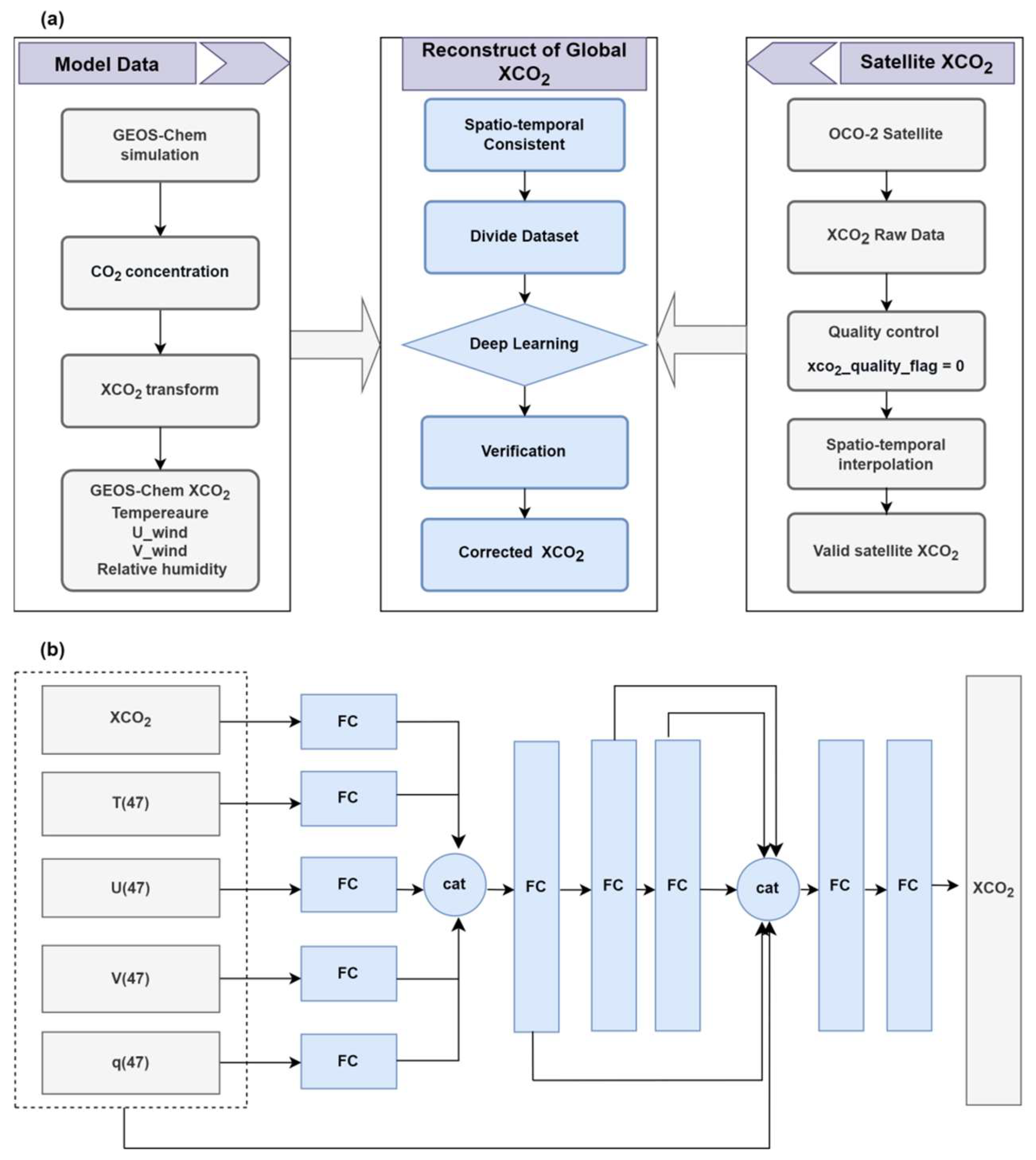
2.2.1. Main Framework

The total surface CO₂ flux will be corrected by a deep learning method, which consists of two neural network models. Figure 2 illustrates the proposed framework for correcting CO₂ flux. The process involves the following steps:

Step 1: Training a concentration correction model. The fully connected model was trained using 3-hour-averaged GEOS-Chem model outputs, which included meteorological data, CO₂ concentration, and satellite observation data. In the training process, the satellite observations served as the training target, while the meteorological data and CO₂ concentration acted as the auxiliary data. The purpose of this training is to refine the results of the GEOS-Chem simulation by integrating satellite observations to enhance the precision of global CO₂ concentration data. Consequently, this model is referred to as the CO₂ concentration correction model.

Step 2: Training a concentration–flux inversion model. The U-net model was trained using 3-hour-averaged GEOS-Chem model outputs, including meteorological data, CO₂ flux data, and CO₂ concentration. The purpose of this training was to enable the U-net model to learn and establish the relationship between CO₂ concentration and CO₂ flux. This model is referred to as the concentration–flux inversion model. In the training process, the CO₂ flux served as the training target, while the meteorological data and CO₂ concentration were used as auxiliary data.

Step 3: Updating the CO₂ flux. Once the well-trained CO₂ concentration correction model and concentration–flux inversion model were obtained, the 3-hour-averaged CO₂ concentration and meteorological data were input into the well-trained CO₂ concentration correction model to generate the optimized global CO₂ concentration. These optimized global CO₂ concentrations, along with the meteorological data, were then input into the well-trained concentration–flux inversion model to generate the posterior CO₂ flux.

2.2.2. Concentration Correction Model

Figure 3 shows the structure for establishing the CO₂ concentration correction model, which is based on simulated data from GEOS-Chem and observed CO₂ concentrations from OCO-2 (Figure 3a). For satellite observations, quality control and spatio-temporal interpolation are performed as described in Section 2.1.2. For GEOS-Chem data, the XCO₂ is obtained as described in Section 2.1.1, and all simulation data are resampled to match the locations of satellite observations. This ensures a consistent dataset in both space and time for observed and simulated data. It should be noted that the calculation of GEOS-Chem XCO₂ and OCO-2 XCO₂ is somewhat different because XCO₂ retrieved from OCO-2 requires both the satellite column averaging kernel and the a priori profile [39]. However, this algorithmic bias will also be corrected in this CO₂ correction model. The dataset from 2015 to 2017 was used for model training, the 2018 dataset was used for model validation, and the 2019 dataset was used for testing. Consequently, the training dataset consists of 438,458 grid points, while the validation and test datasets consist of 167,316, and 162,530 grid points, respectively.

The CO₂ concentration correction model is based on a fully connected neural network (Figure 3b). We constructed a multi-input deep learning architecture. This model first receives data from multiple features, processes each feature through locally fully connected (FC) layers, and then concatenates them. The concatenated feature vector passes through three FC layers and is combined with the initial single-level input features, further enriching the model’s representational capacity. Subsequently, all feature vectors are processed through two additional FC layers, with the final output used to predict CO₂ concentration.

The input layer comprises 47 levels each for temperature profile, humidity profile, and meridional and zonal wind profile, as well as one layer for simulated XCO₂, resulting in a total of 189 neurons. The output layer represents the OCO-2 CO₂ concentration. The Adam optimizer was used, and mean squared error (MSE) was chosen as the loss function, with an initial learning rate of 0.001. The batch size was set to 128, and the number of epochs was set to 100.

2.2.3. Concentration–Flux Inversion Model

The concentration–flux inversion model is based on a U-Net neural network. U-Net is an advanced form of convolutional neural network (CNN) model that was originally proposed to solve medical image segmentation problems. Its main feature is a “U”-shaped network structure that can effectively utilize neighbor information to achieve pixel-level prediction [46]. The U-Net structure (5 layers), illustrated in Figure 4, comprises two parts: the left half represents the encoding path and the right half represents the decoding path. The encoding path consists of five convolutional layers and pooling layers, which are used to extract features from the image. The decoding path consists of five upsampling layers and convolutional layers, which are used to upsample and merge feature maps. Furthermore, skip connections in the network preserve the high-resolution information extracted during the encoding path and transmit it to the corresponding upsampling layers to retain features of different scale spatial fields.

In our concentration–flux inversion model based on the U-Net neural network, the output layer represents the CO₂ flux with dimensions of 91 by 144. The size of the input image is (91, 144, 64); thus, the input layer consists of 64 features. These features consist of 15 levels each of temperature profiles, humidity profiles, and meridional and zonal wind profiles, one level of boundary layer height, one level of shortwave radiation, and two time steps (current and next time steps) of CO₂ concentration. Note that the change in CO₂ concentration is determined by fluxes and other meteorological fields, so the current and next time steps of CO₂ concentration are a good indication of the value of CO₂ fluxes. Meanwhile, we selected 15 out of the 47 layers of meteorological profile features for model training to increase the efficiency and reduce the computational resources. The difference in current and next time steps of CO₂ concentration and all layers of meteorological profile features were used to train the model, and the model showed similar performance. The U-Net model was trained on data from 2015 to 2017, with 2018 data serving as the validation set. Data from 2019 were used as the test dataset to validate the performance of the concentration–flux inversion model. Thus, the length of the training, validation, and test sets is 8768, 2920, and 2920, respectively.

The Rectified Linear Unit (ReLU) function is used as the activation function, and Root Mean Square prop (RMSprop) is selected as the optimizer. The convolution and pooling kernel sizes are set to 3 × 3 and 2 × 2, respectively. Mean absolute error (MAE) is used as the loss function, with an initial learning rate of 0.001. The batch size is set to 64, and the number of epochs is set to 500.

3. Results

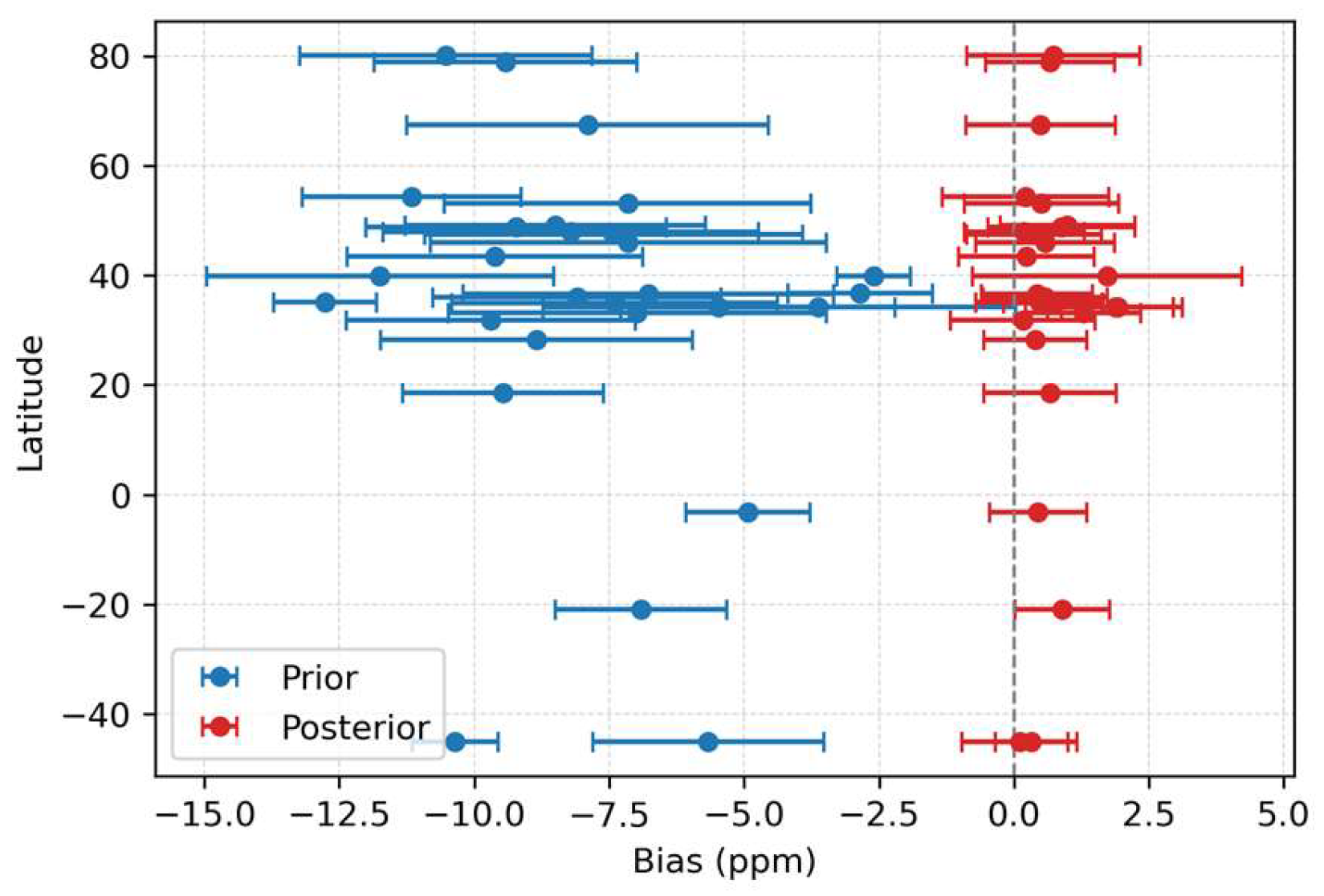
3.1. Performance of Concentration Correction Model

Due to inaccuracies in the prior CO₂ fluxes, the prior CO₂ concentrations simulated by the GEOS-Chem model are also inaccurate and deviate significantly from the observed satellite observations. As shown in Figure 5a, the mean bias of CO₂ concentrations between satellite observations and the GEOS-Chem simulation is −11.406 ppm and the standard deviation is 1.808 ppm. Traditional methods use data assimilation techniques to continuously improve model-estimated CO₂ concentrations, reducing the bias between simulated and observed CO₂ concentrations by integrating satellite and ground-based observations [10,17,19]. In contrast, our approach directly uses OCO-2 CO₂ concentrations to reduce model biases with a data-driven correction model. Our approach demonstrates that the discrepancy between satellite observations and predicted CO₂ concentrations by the concentration correction model is significantly reduced, with a mean bias of 0.461 ppm and a standard deviation of 1.673 ppm (Figure 5b). The RMSE and MAE after our correction are 1.735 ppm and 1.195 ppm, respectively, representing a reduction compared to values before correction. To verify the model’s performance across different seasons, Figure 6 shows the seasonal mean bias. As can be seen, the concentration correction model significantly reduces the mean bias to zero in each season. These results suggest that the prior CO₂ concentrations simulated by the GEOS-Chem model can be effectively corrected by the CO₂ concentration correction model.

3.2. Performance of the Concentration–Flux Inversion Model

The performance of the U-Net model was evaluated to determine whether it had learned the relationship between concentration and flux. Figure 7 displays the prior and predicted distributions of the annual mean CO₂ flux for the validated period. All indicators demonstrate excellent performance, with a correlation coefficient (COR) of 0.966, MAE of 0.038 kg·m⁻² yr⁻¹, and root mean square error (RMSE) of 0.087 kg·m⁻² yr⁻¹. Additionally, annual and seasonal mean statistics were calculated to assess whether the model performance was time- and sample-dependent.

Table 2. Performance of the U-Net model for annual data and data from each season (COR: correlation coefficient; MAE: mean absolute error, unit: kg·m⁻² yr⁻¹; RMSE: root mean squared error, unit: kg·m⁻² yr⁻¹).

	Annual	Spring	Summer	Autumn	Winter
COR	0.920	0.920	0.906	0.921	0.931
MAE	0.226	0.209	0.331	0.194	0.167
RMSE	0.899	0.842	1.235	0.796	0.719

presents the validation performance for annual data and data for different seasons. Overall, the results show impressive performance in all indicators, with an annual average COR of 0.920, MAE of 0.226 kg·m⁻² yr⁻¹, and RMSE of 0.899 kg·m⁻² yr⁻¹. The concentration–flux inversion model performed most favorably in winter, with a COR of 0.931 and MAE and RMSE of only 0.167 kg·m⁻² yr⁻¹ and 0.719 kg·m⁻² yr⁻¹, respectively. And the performance in summer is slightly worse than in other seasons. Nonetheless, the overall performance of the concentration–flux inversion model is satisfactory. This indicates that the U-Net is capable of accurately capturing the relationship within an acceptable bias, making it suitable for flux adjustment.

3.3. Surface CO₂ Flux Updating and Analysis

By combining the well-trained concentration correction model and the concentration–flux inversion model, optimized CO₂ flux can be obtained through a two-step correction process. In the first step, the well-trained concentration correction model is used to correct the prior CO₂ concentration simulated by the GEOS-Chem model, resulting in accurate global high-temporal-resolution posterior CO₂ concentration data. In the second step, the corrected posterior CO₂ concentration, along with the atmospheric profiles, is used to construct a dataset to drive the well-trained concentration–flux inversion model, yielding the globally corrected posterior CO₂ flux. The optimized CO₂ flux is compared with the results of other two advanced atmospheric inversion systems, namely, CAMS [44] and CT2022 [45], which use different atmospheric transport models and data assimilation techniques and assimilate different types of CO₂ observations.

3.3.1. CO₂ Concentration Updating

Figure 8 shows the correction of CO₂ concentration. The Lamont, Garmisch, and Hefei stations from TCCON were chosen as examples because they have sufficient observational data and are located in the Americas, Europe, and Asia, respectively. Due to the inaccuracies in the prior CO₂ flux driving the GEOS-Chem model, the simulated prior CO₂ concentration growth rate is significantly higher than the rate observed by TCCON. For instance, the observed growth rates of annual mean CO₂ concentration from 2015 to 2019 at the Lamont, Garmisch, and Hefei stations are 2.17 ppm yr⁻¹, 1.97 ppm yr⁻¹, and 1.83 ppm yr⁻¹, respectively (Figure 8a–c). However, the simulated growth rates of annual mean CO₂ for GEOS-Chem in these stations are approximately 1.5 times higher than those observed by the ground-based measurements, at 3.17 ppm yr⁻¹, 3.14 ppm yr⁻¹, and 3.22 ppm yr⁻¹, respectively. As a result, the difference between the prior CO₂ concentration simulated by GEOS-Chem and the observations continues to grow. Using the concentration correction model, CO₂ concentration is optimized to a normal range, with a bias between −5 and 5 ppm from ground-based observations (Figure 8d–f).

Additionally, Figure 9 presents a comparison of CO₂ concentrations for each TCCON site across different latitudes. The bias values of the prior CO₂ concentration are quite large, with a global mean of −7.87 ppm. In contrast, the bias values of the posterior CO₂ concentration at most sites are reduced to within 1 ppm, with a global mean of 0.68 ppm. These results confirmed the reliability of the corrected posterior CO₂ concentration data.

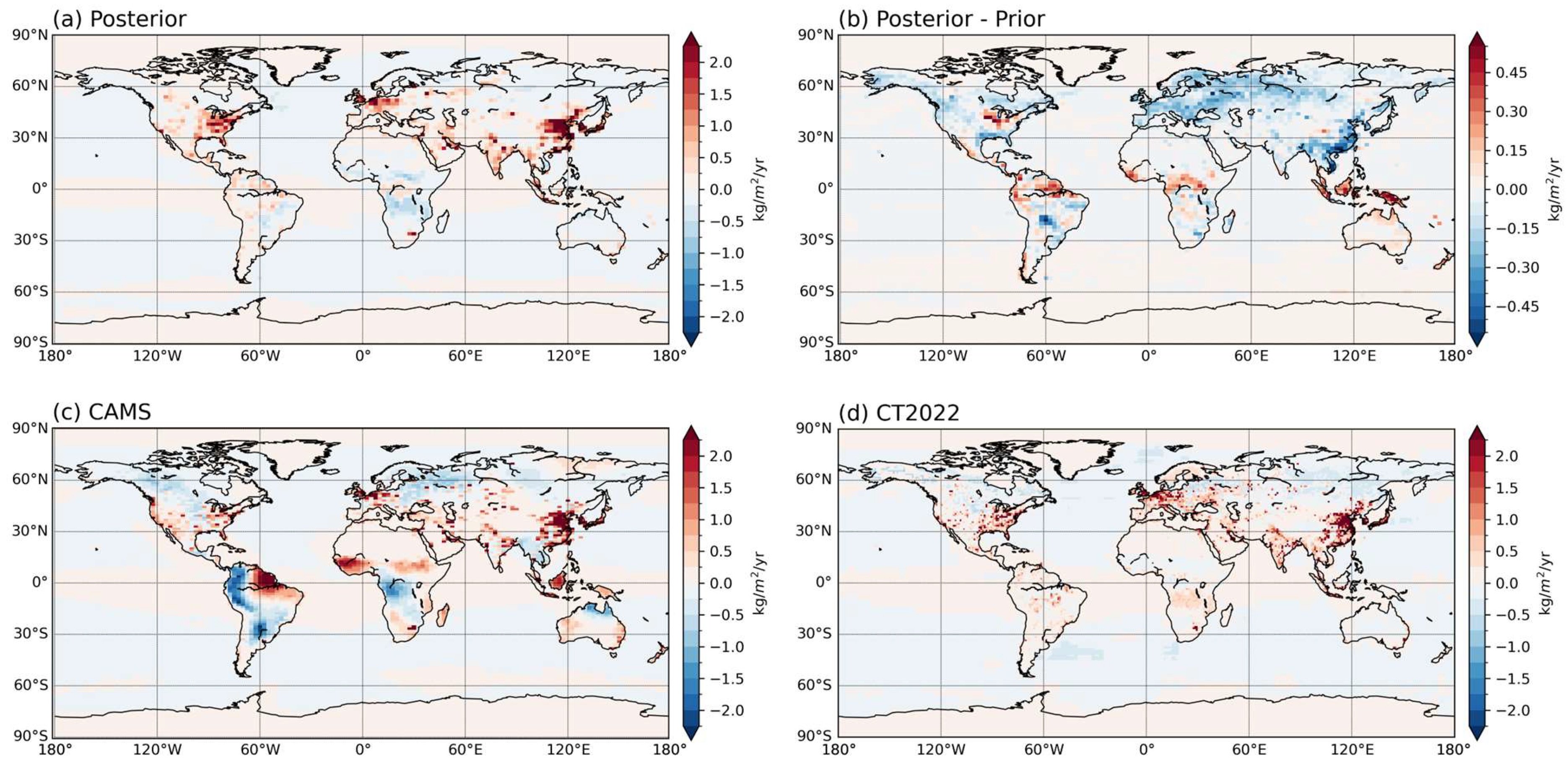
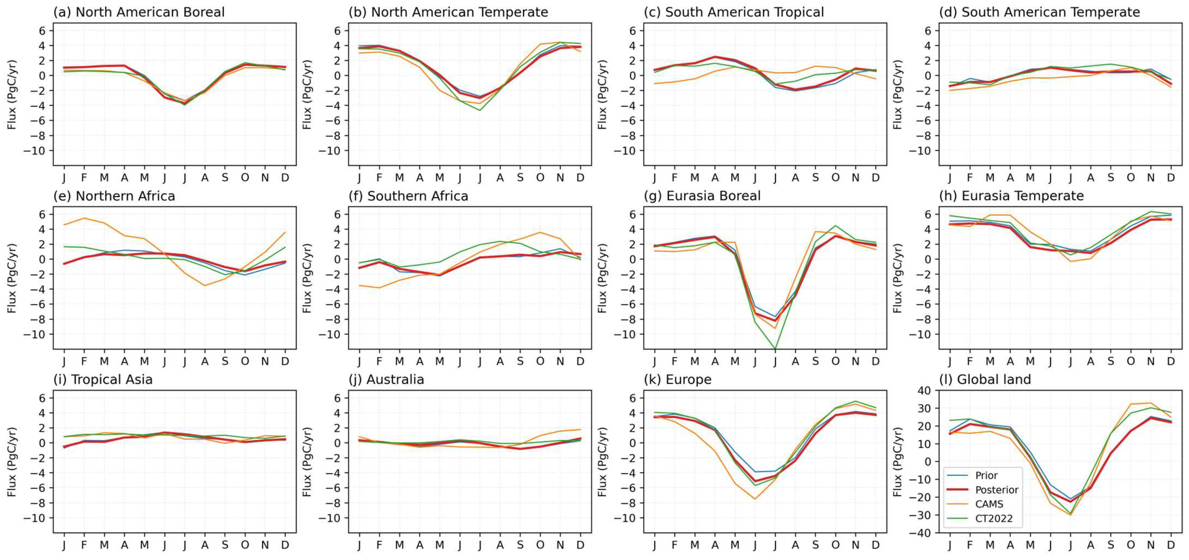
3.3.2. Surface Total CO₂ Flux Analysis

Based on the corrected posterior CO₂ concentration and well-trained concentration–flux inversion model, the corrected posterior CO₂ flux can be obtained. Figure 10 presents the spatial distribution of the annual average posterior CO₂ flux for the period from 2015 to 2019 derived from our inversion model, as well as the difference between prior and posterior fluxes. Compared to the prior CO₂ flux, the posterior CO₂ flux has been optimized mainly in land regions, with little adjustment in oceanic regions (Figure 10b). Notably, the posterior land flux decreases significantly in most parts of the Eurasia boreal region and the eastern part of China, while it increases in equatorial Africa, equatorial South America, and maritime continental.

In addition, our posterior CO₂ flux was compared with the estimations from CAMS and CT2022. It is important to note that there are systematic differences in the CO₂ flux obtained from different inversions between CAMS and CT2022 (Figure 10c,d), which may be due to the different observations and prior fluxes used. Previous studies found that the different choices of terrestrial CO₂ fluxes [37], emission inventories [47], and whether ground-based or satellite observations are assimilated [48], can all lead to varying flux distributions in the inversion.

Overall, the distribution of our posterior CO₂ flux was broadly consistent with that of CT2022 (Figure 10a,d). Furthermore, we estimated the carbon flux over the 11 TransCom land regions (Figure 11). The results indicate that large carbon sources are located in the Eurasia Temperate, North American Temperate, and Tropical Asia regions due to anthropogenic carbon emissions. Compared to prior flux, these large carbon sources have been reduced in our posterior estimation. There is minimal difference between the prior and posterior estimations of CO₂ flux in Tropical Asia. However, it is important to highlight that the carbon source is augmented in the maritime continental region, while there is a significant decrease in China (Figure 10b). CAMS shows a large carbon source in Northern Africa and a large sink in South American Temperate, which is not displayed in our inversion and CT2022.

Figure 12 shows the seasonal cycle of CO₂ fluxes over the 11 TransCom regions. Predominant sinks were identified during the growing season, with maximum monthly sinks occurring in June and July in the Northern Hemisphere regions, including the North American Boreal (Figure 12a), North American Temperate (Figure 12b), Eurasian Boreal (Figure 12g), and Europe (Figure 12k) regions. Our results exhibited seasonal cycle amplitudes similar to those of the other two inversion models.

4. Discussion

Traditional carbon assimilation methods often demand substantial computational resources, while machine learning and deep learning techniques have been increasingly applied to enhance efficiency. In this context, we propose a novel “top-down” global carbon flux correction method based on deep learning, comprising two neural network models. The first model is a CO₂ concentration correction model, designed to refine the results of GEOS-Chem simulations using satellite observations. It is important to note that discrepancies exist between the GEOS-Chem XCO₂ and OCO-2 XCO₂ calculations; however, these differences are implicitly addressed in the bias calibration of the correction model. The second model is a concentration–flux inversion model, which establishes a complex mapping relationship between flux and concentration.

This work is a new attempt at utilizing satellite data for carbon flux correction based on deep learning technology, and there may be some issues that should be addressed and need to be improved in future research. Firstly, the current availability and accuracy of satellite data may limit the CO₂ concentration correction model’s precision. With the development of carbon satellites in the future, the correction model is likely to see significant improvements. Secondly, results indicate that the performance of our concentration–flux inversion model varies across different seasons, demonstrating superior performance in winter and lower performance in summer. Further development of advanced deep learning algorithms is necessary to enhance model performance. For instance, our current U-Net model primarily considers spatial connection while ignoring the temporal linkage. In future work, combining CNNs with recurrent neural networks (RNNs) could better capture the relationship between CO₂ fluxes and concentrations. Additionally, other advanced methods like Transformers are also being considered, which could further enhance the model’s capabilities. Thirdly, the uncertainty in the final CO₂ flux has not been thoroughly analyzed, particularly regarding the impact of observational errors, since satellite data usually have large uncertainties. Although evaluating the accuracy and uncertainty of gridded emissions is challenging due to the lack of direct physical measurements at grid scales, future efforts should focus on this issue. Experiments using different observational error covariance settings are planned to assess the sensitivity of flux results to various configurations, thereby indirectly estimating the associated uncertainties. Finally, the total surface CO₂ flux was optimized in our deep learning model, because the influence of different fluxes on concentration is difficult to separate. However, the distinction between anthropogenic CO₂ emissions and natural sinks remains a key concern. Therefore, a multi-task model is planned for future development, to achieve the simultaneous optimization of different carbon fluxes.

Currently, data assimilation remains the mainstream approach for solving carbon inversions, but this work provides a new perspective for “top-down” carbon estimation studies, despite the current limitations of our deep learning models. This deep learning method can serve as a valuable complement to traditional approaches and has potential applications in a broader range of fields, including the correction of pollutant inventories. As research progresses, this approach is expected to evolve into a more effective tool for estimating CO₂ and other fluxes in the future.

5. Conclusions

Top-down methods for constraining surface carbon fluxes from satellite CO₂ observations have great potential for estimating surface carbon fluxes, particularly in areas with limited coverage by existing ground-based CO₂ observation networks. However, existing top-down assimilation inversion methods based on data assimilation have some limitations, especially in terms of computational resources. Therefore, this study aims to develop a new method for carbon flux revision based on deep learning and satellite observations. This approach relies on two deep learning models trained using satellite observations and atmospheric chemistry transport model data: a CO₂ concentration correction model and a concentration–flux inversion model. First, the optimized global CO₂ concentration is obtained by correcting the prior CO₂ concentration simulated by the atmospheric chemistry transport model using the well-trained concentration correction model. Then, the optimized posterior CO₂ flux is derived through the well-trained concentration–flux inversion model. Our posterior estimation of the total surface CO₂ flux is reduced in the Eurasian boreal region and eastern China. The general distribution of our posterior CO₂ flux is relatively similar to that of CT2022 and CMAS, although some discrepancies remain. Previous studies have highlighted that the choice of observations, atmospheric chemical transport models, and prior fluxes can contribute to discrepancies among different methods. Further investigation such as OSSEs (observation system simulation experiments) is necessary to determine whether these factors impact our model’s results and lead to deviations from other methods.

References

1. IPCC. Climate Change 2014: Synthesis Report; Cambridge University Press: Cambridge, UK; New York, NY, USA, 2014. [Google Scholar]
2. UNFCCC. Adoption of the Paris Agreement; United Nations Framework Convention on Climate Change; UN: Paris, France, 2015; Available online: https://unfccc.int/resource/docs/2015/cop21/eng/l09r01.pdf (accessed on 11 September 2023).
3. IPCC. Climate Change 2021: The Physical Science Basis; Cambridge University Press: Cambridge, UK, 2021. [Google Scholar]
4. Feng, R.; Hu, L.; Hu, X.; Fang, X. Knowledge gaps are making it harder to formulate national climate policies. Proc. Natl. Acad. Sci. USA 2023, 120, e2218563120. [Google Scholar] [CrossRef] [PubMed]
5. Liu, Z.; Guan, D.; Wei, W.; Davis, S.; Ciais, P.; Bai, J.; Peng, S.; Zhang, Q.; Klaus, H.; Marland, G.; et al. Reduced carbon emission estimates from fossil fuel combustion and cement production in China. Nature 2015, 524, 335–338. [Google Scholar] [CrossRef] [PubMed]
6. Korsbakken, J.I.; Peters, G.P.; Andrew, R.M. Uncertainties around reductions in China’s coal use and CO2 emissions. Nat. Clim. Chang. 2016, 6, 687–690. [Google Scholar] [CrossRef]
7. Piao, S.; He, Y.; Wang, X.; Chen, F. Estimation of China’s terrestrial ecosystem carbon sink: Methods, progress and prospects. Sci. China Earth Sci. 2022, 65, 641–651. [Google Scholar] [CrossRef]
8. Wang, J.; Feng, L.; Palmer, P.I.; Liu, Y.; Fang, S.; Tang, X.; Yang, D.; Liu, L.; Xia, C. Large Chinese land carbon sink estimated from atmospheric carbon dioxide data. Nature 2020, 586, 720–723. [Google Scholar] [CrossRef]
9. Zhang, S.; Zheng, X.; Chen, J.M.; Chen, Z.; Dan, B.; Yi, X.; Wang, L.; Wu, G. A global carbon assimilation system using a modified ensemble Kalman filter. Geosci. Model Dev. 2015, 8, 805–816. [Google Scholar] [CrossRef]
10. Jiang, F.; Wang, H.; Chen, J.M.; Ju, W.; Tian, X.; Feng, S.; Li, G.; Chen, Z.; Zhang, S.; Lu, X.; et al. Regional CO2 fluxes from 2010 to 2015 inferred from GOSAT XCO2 retrievals using a new version of the Global Carbon Assimilation System. Atmos. Chem. Phys. 2021, 21, 1963–1985. [Google Scholar] [CrossRef]
11. Tian, X.; Xie, Z.; Cai, Z.; Liu, Y.; Fu, Y.; Zhang, H. The Chinese carbon cycle data-assimilation system (Tan-Tracker). Chin. Sci. Bull. 2014, 59, 1541–1546. [Google Scholar] [CrossRef]
12. Schürmann, G.J.; Kaminski, T.; Köstler, C.; Carvalhais, N.; Voßbeck, M.; Kattge, J.; Giering, R.; Rödenbeck, C.; Heimann, M.; Zaehle, S. Constraining a land-surface model with multiple observations by application of the MPI-Carbon Cycle Data Assimilation System V1.0. Geosci. Model Dev. 2016, 9, 2999–3026. [Google Scholar] [CrossRef]
13. Zhang, H.F.; Chen, B.Z.; van der Laan-Luijkx, I.T.; Chen, J.; Xu, G.; Yan, J.W.; Zhou, L.X.; Fukuyama, Y.; Tans, P.P.; Peters, W. Net terrestrial CO2 exchange over China during 2001–2010 estimated with an ensemble data assimilation system for atmospheric CO2. J. Geophys. Res. Atmos. 2014, 119, 3500–3515. [Google Scholar] [CrossRef]
14. Luijkx, I.; Velde, I.; Veen, E.; Tsuruta, A.; Stanisławska, K.; Babenhauserheide, A.; Zhang, H.; Liu, Y.; He, W.; Chen, H.; et al. The CarbonTracker Data Assimilation Shell (CTDAS) v1.0: Implementation and global carbon balance 2001–2015. Geosci. Model Dev. 2017, 10, 2785–2800. [Google Scholar] [CrossRef]
15. Peters, W.; Krol, M.; Werf, G.; Houweling, S.; Jones, C.; Hughes, J.; Schaefer, K.; Masarie, K.; Jacobson, A.; Miller, J.; et al. Seven years of recent European net terrestrial carbon dioxide exchange constrained by atmospheric observations. Glob. Chang. Biol. 2010, 16, 1317–1337. [Google Scholar] [CrossRef]
16. Peters, W.; Jacobson, A.; Sweeney, C.; Andrews, A.; Conway, T.; Masarie, K.; Miller, J.; Bruhwiler, L.; Petron, G.; Hirsch, A.; et al. An atmospheric perspective on North American carbon dioxide exchange: CarbonTracker. Proc. Natl. Acad. Sci. USA 2007, 104, 18925–18930. [Google Scholar] [CrossRef]
17. Peters, W.; Miller, J.B.; Whitaker, J.; Denning, A.S.; Hirsch, A.; Krol, M.C.; Zupanski, D.; Bruhwiler, L.; Tans, P.P. An ensemble data assimilation system to estimate CO2 surface fluxes from atmospheric trace gas observations. J. Geophys. Res. Atmos. 2005, 110, D24304. [Google Scholar] [CrossRef]
18. Miyazaki, K.; Maki, T.; Patra, P.; Nakazawa, T. Assessing the impact of satellite, aircraft, and surface observations on CO2 flux estimation using an ensemble-based 4-D data assimilation system. J. Geophys. Res. 2011, 116, D16306. [Google Scholar] [CrossRef]
19. Kong, Y.; Zheng, B.; Zhang, Q.; He, K. Global and regional carbon budget for 2015–2020 inferred from OCO-2 based on an ensemble Kalman filter coupled with GEOS-Chem. Atmos. Chem. Phys. 2022, 22, 10769–10788. [Google Scholar] [CrossRef]
20. Lin, X.; Ma, J.; Chen, H.; Shen, F.; Ahmad, S.; Li, Z. Carbon Emissions Estimation and Spatiotemporal Analysis of China at City Level Based on Multi-Dimensional Data and Machine Learning. Remote Sens. 2022, 14, 3014. [Google Scholar] [CrossRef]
21. Li, Y.; Chen, Y.; Cai, Q.; Zhu, L. Calculation of CO2 Emissions from China at Regional Scales Using Remote Sensing Data. Remote Sens. 2024, 16, 544. [Google Scholar] [CrossRef]
22. Zhang, M.; Liu, G. Mapping contiguous XCO2 by machine learning and analyzing the spatio-temporal variation in China from 2003 to 2019. Sci. Total Environ. 2023, 858, 159588. [Google Scholar] [CrossRef]
23. Zhang, L.; Li, T.; Wu, J. Deriving gapless CO2 concentrations using a geographically weighted neural network: China, 2014–2020. Int. J. Appl. Earth Obs. Geoinf. 2022, 114, 103063. [Google Scholar] [CrossRef]
24. Hua, Y.; Zhao, X.; Sun, W.; Sun, Q. Satellite-Based Reconstruction of Atmospheric CO2 Concentration over China Using a Hybrid CNN and Spatiotemporal Kriging Model. Remote Sensing 2024, 16, 2433. [Google Scholar] [CrossRef]
25. Huang, L.; Liu, S.; Yang, Z.; Xing, J.; Zhang, J.; Bian, J.; Li, S.; Sahu, S.K.; Wang, S.; Liu, T.Y. Exploring deep learning for air pollutant emission estimation. Geosci. Model Dev. 2021, 14, 4641–4654. [Google Scholar] [CrossRef]
26. Feng, X.; Fu, T.-M.; Cao, H.; Tian, H.; Fan, Q.; Chen, X. Neural network predictions of pollutant emissions from open burning of crop residues: Application to air quality forecasts in southern China. Atmos. Environ. 2019, 204, 22–31. [Google Scholar] [CrossRef]
27. Chen, Y.; Fung, J.C.H.; Yuan, D.; Chen, W.; Fung, T.; Lu, X. Development of an integrated machine-learning and data assimilation framework for NOx emission inversion. Sci. Total Environ. 2023, 871, 161951. [Google Scholar] [CrossRef]
28. Bey, I.; Jacob, D.; Yantosca, R.; Logan, J.; Field, B.; Fiore, A.; Li, Q.-B.; Liu, H.; Mickley, L.; Schultz, M. Global Modeling of Tropospheric Chemistry with Assimilated Meteorology: Model Description and Evaluation. J. Geophys. Res. Atmos. 2001, 106, 23073–23095. [Google Scholar] [CrossRef]
29. Nassar, R.; Jones, D.; Kulawik, S.; Worden, J.; Bowman, K.; Andres, R.; Suntharalingam, P.; Chen, J.; Brenninkmeijer, C.; Schuck, T.; et al. Inverse modeling of CO2 sources and sinks using satellite observations of CO2 from TES and surface flask measurements. Atmos. Chem. Phys. 2011, 11, 6029–6047. [Google Scholar] [CrossRef]
30. Oda, T.; Maksyutov, S. A very high-resolution (1 km×1 km) global fossil fuel CO2 emission inventory derived using a point source database and satellite observations of nighttime lights. Atmos. Chem. Phys. 2011, 11, 543–556. [Google Scholar] [CrossRef]
31. Oda, T.; Maksyutov, S.; Andres, R.J. The Open-source Data Inventory for Anthropogenic CO2, version 2016 (ODIAC2016): A global monthly fossil fuel CO2 gridded emissions data product for tracer transport simulations and surface flux inversions. Earth Syst. Sci. Data 2018, 10, 87–107. [Google Scholar] [CrossRef]
32. Nassar, R.; Napier-Linton, L.; Gurney, K.R.; Andres, R.J.; Oda, T.; Vogel, F.R.; Deng, F. Improving the temporal and spatial distribution of CO2 emissions from global fossil fuel emission data sets. J. Geophys. Res. Atmos. 2013, 118, 917–933. [Google Scholar] [CrossRef]
33. van der Werf, G.R.; Randerson, J.T.; Giglio, L.; van Leeuwen, T.T.; Chen, Y.; Rogers, B.M.; Mu, M.; van Marle, M.J.E.; Morton, D.C.; Collatz, G.J.; et al. Global fire emissions estimates during 1997–2016. Earth Syst. Sci. Data 2017, 9, 697–720. [Google Scholar] [CrossRef]
34. Pan, X.; Ichoku, C.; Chin, M.; Bian, H.; Darmenov, A.; Colarco, P.; Ellison, L.; Kucsera, T.; da Silva, A.; Wang, J.; et al. Six global biomass burning emission datasets: Intercomparison and application in one global aerosol model. Atmos. Chem. Phys. 2020, 20, 969–994. [Google Scholar] [CrossRef]
35. Iida, Y.; Takatani, Y.; Kojima, A.; Ishii, M. Global trends of ocean CO2 sink and ocean acidification: An observation-based reconstruction of surface ocean inorganic carbon variables. J. Oceanogr. 2021, 77, 323–358. [Google Scholar] [CrossRef]
36. Ott, L. GEOS-Carb CASA-GFED 3-Hourly Ecosystem Exchange Fluxes 0.5 Degree x 0.625 Degree V3; Goddard Earth Sciences Data and Information Services Center (GES DISC): Greenbelt, MD, USA, 2022.
37. Philip, S.; Johnson, M.S.; Potter, C.; Genovesse, V.; Baker, D.F.; Haynes, K.D.; Henze, D.K.; Liu, J.; Poulter, B. Prior biosphere model impact on global terrestrial CO2 fluxes estimated from OCO-2 retrievals. Atmos. Chem. Phys. 2019, 19, 13267–13287. [Google Scholar] [CrossRef]
38. Peiro, H.; Crowell, S.; Moore Iii, B. Optimizing 4 years of CO2 biospheric fluxes from OCO-2 and in situ data in TM5: Fire emissions from GFED and inferred from MOPITT CO data. Atmos. Chem. Phys. 2022, 22, 15817–15849. [Google Scholar] [CrossRef]
39. Connor, B.J.; Boesch, H.; Toon, G.; Sen, B.; Miller, C.; Crisp, D. Orbiting Carbon Observatory: Inverse method and prospective error analysis. J. Geophys. Res. Atmos. 2008, 113, D05305. [Google Scholar] [CrossRef]
40. Crisp, D.; Atlas, R.M.; Breon, F.M.; Brown, L.R.; Burrows, J.P.; Ciais, P.; Connor, B.J.; Doney, S.C.; Fung, I.Y.; Jacob, D.J.; et al. The Orbiting Carbon Observatory (OCO) mission. Adv. Space Res. 2004, 34, 700–709. [Google Scholar] [CrossRef]
41. Hakkarainen, J.; Ialongo, I.; Tamminen, J. Direct space-based observations of anthropogenic CO2 emission areas from OCO-2. Geophys. Res. Lett. 2016, 43, 11400–11406. [Google Scholar] [CrossRef]
42. Zhang, S.; Bai, Y.; He, X.; Huang, H.; Zhu, Q.; Gong, F. Comparisons of OCO-2 satellite derived XCO2 with in situ and modeled data over global ocean. Acta Oceanol. Sin. 2021, 40, 136–142. [Google Scholar] [CrossRef]
43. Hong, X.; Zhang, P.; Bi, Y.; Liu, C.; Sun, Y.; Wang, W.; Chen, Z.; Hao, Y.; Zhang, C.; Yuan, T.; et al. Retrieval of Global Carbon Dioxide From TanSat Satellite and Comprehensive Validation With TCCON Measurements and Satellite Observations. IEEE Trans. Geosci. Remote Sens. 2021, 60, 1–16. [Google Scholar] [CrossRef]
44. Chevallier, F.; Fisher, M.; Peylin, P.; Serrar, S.; Bousquet, P.; Breon, F.-M.; Chedin, A.; Ciais, P. Inferring CO2 sources and sinks from satellite observations: Method and application to TOVS data. J. Geophys. Res. 2005, 110, D24309. [Google Scholar] [CrossRef]
45. Jacobson, A.R.; Schuldt, K.N.; Tans, P.; Arlyn, A.; Miller, J.B.; Oda, T.; Mund, J.; Weir, B.; Ott, L.; Aalto, T.; et al. CarbonTracker CT2022; NOAA Global Monitoring Laboratory: Boulder, CO, USA, 2023. [Google Scholar]
46. Ronneberger, O.; Fischer, P.; Brox, T. U-Net: Convolutional Networks for Biomedical Image Segmentation. In Medical Image Computing and Computer-Assisted Intervention—MICCAI 2015; Springer: Cham, Switzerland, 2015. [Google Scholar]
47. Jin, Z.; Wang, T.; Zhang, H.; Wang, Y.; Ding, J.; Tian, X. Constraint of satellite CO2 retrieval on the global carbon cycle from a Chinese atmospheric inversion system. Sci. China Earth Sci. 2023, 66, 609–618. [Google Scholar] [CrossRef]
48. Chevallier, F.; Remaud, M.; O’Dell, C.W.; Baker, D.; Peylin, P.; Cozic, A. Objective evaluation of surface- and satellite-driven carbon dioxide atmospheric inversions. Atmos. Chem. Phys. 2019, 19, 14233–14251. [Google Scholar] [CrossRef]
Figure 1. Distribution of GEOS-Chem simulated XCO2, OCO-2 observed XCO2, and ground-based observation sites. Displayed are the distribution of (a) GEOS-Chem simulated XCO2 and (b) original OCO-2-observed XCO2 retrievals on 1 January 2015. The “N” in the upper right corner of (b) indicates the number of valid grids. Red stars in (c) represent the 30 TCCON sites used for evaluation, and the shading indicates the 11 TransCom land regions.
Remotesensing 16 03694 g001
Figure 2. The framework for correcting CO2 flux based on deep learning.
Remotesensing 16 03694 g002
Figure 3. The (a) data preprocessing and (b) fully connected neural network structure for CO2 concentration correction model.
Remotesensing 16 03694 g003
Figure 4. The structure of concentration–flux inversion model based on U-Net neural network.
Remotesensing 16 03694 g004
Figure 5. The validation performance of the concentration correction model. The distribution of (a) differences between satellite-observed and GEOS-Chem-simulated CO2 concentration, and (b) differences between satellite-observed and model-predicted CO2 concentration are shown.
Remotesensing 16 03694 g005
Figure 6. Performance of the concentration correction model for each season. Boxplots show the mean bias of the valid grid in annual, spring, summer, autumn, and winter (a) before correction and (b) after correction.
Remotesensing 16 03694 g006
Figure 7. The validation performance of the concentration–flux inversion model. Shown are the annual mean of (a) prior CO2 flux and (b) predicted CO2 flux by concentration-flux inversion model.
Remotesensing 16 03694 g007
Figure 8. Comparisons between corrected posterior CO2 concentration and three TCCON retrievals. Left panels show the time series of prior (blue), posterior (red), and observed XCO2 (black) for (a) Lamont station in the Americas, (b) Garmisch station in Europe, and (c) Hefei station in Asia. The right panels show the corresponding probability distribution of the bias between observation and prior XCO2 (blue), and the bias between observation and posterior XCO2 (red) for (d) Lamont, (e) Garmisch, and (f) Hefei, respectively.
Remotesensing 16 03694 g008
Figure 9. Comparison of CO2 concentration with all TCCON retrievals. The error bar displays the bias distribution between ground-based observation and prior XCO2 (blue), and the bias between observation and posterior XCO2 (red) for all TCCON stations at different latitudes.
Remotesensing 16 03694 g009
Figure 10. Global distributions of annual mean CO2 flux from 2015 to 2019 for (a) the posterior, (b) the difference of posterior and prior, (c) the CAMS, and (d) CT2022, respectively.
Remotesensing 16 03694 g010
Figure 11. Surface CO2 fluxes derived over the 11 TransCom land regions. Bars with different colors represent the surface CO2 fluxes averaged from 2015 to 2019 for each TransCom land region. Blue, orange, green, and red bars represent our prior and posterior surface CO2 fluxes, and estimations of CT2022 and CAMS, respectively.
Remotesensing 16 03694 g011
Figure 12. Seasonal cycle of the surface CO2 fluxes over TransCom regions. The solid curves represent the surface CO2 fluxes averaged from 2015 to 2019 over 11 TransCom land regions from different sources, with colors matching those shown in Figure 10. The x-axis represents the months from January to December.
Remotesensing 16 03694 g012