Analysis of the Grid Quantization for the Microwave Radar Coincidence Imaging Based on Basic Correlation Algorithm

Abstract

In Microwave Radar Coincidence Imaging (MRCI), the imaging region is typically discretized into a fine grid. In other words, it assumes that the equivalent scatterers of the target are precisely located at the centers of these pre-discretized grids. However, this approach usually encounters the off-grid problem, which can significantly degrade the imaging performance. In this paper, to establish a criterion for grid quantization, the performance of the MRCI system related to the grid size and the distribution of imaging points is investigated. First, the discretization of the imaging scene is regarded as a random sampling problem, and the off-grid imaging model for MRCI is established. Then, the probability distribution function (PDF) of the imaging amplitude for a single point target is analyzed, and the mean first-order imaging error (MFE) for multiple point targets is derived based on the Basic Correlation Algorithm (BCA). Finally, the relationship between the grid quantization of the imaging area and the performance of the MRCI system is analyzed, providing a theoretical guidance for enhancing the performance of MRCI. The validity of the analyses is verified through simulation experiments.

1. Introduction

In the past decade, radar imaging has been significantly developed and had various applications [1]. Synthetic Aperture Radar (SAR) and Inverse Synthetic Aperture Radar (ISAR) imaging techniques utilize the Range-Doppler (RD) principle to achieve range-azimuth imaging. High azimuth resolution depends on the temporal accumulation of relative motions [2,3]. However, SAR and ISAR imaging face significant challenges with complex geometric observation scenarios, compounded by the substantial time costs associated with data acquisition and processing. Another conventional radar imaging technique, Phased Array Radar (PAR), can significantly enhance imaging efficiency and quality. Nevertheless, these improvements come at a cost of increased system complexity and limited resolution due to the constrained aperture size. In recent years, there has been a gradual development of new radar technologies, including the Movable-Antenna Multiple Input Multiple Output (MIMO) system [4], Time-Modulated Arrays (TMA) radar system and the Microwave Radar Coincidence Imaging (MRCI) [5]. The MRCI inspired by the optical ghost imaging [6,7], and it demonstrates a promising alternative that has seen rapid development in recent years [8,9,10,11,12,13,14]. Unlike RD-based imaging techniques, MRCI achieves high-resolution imaging through random modulation of radar transmitting signals to construct temporal–spatial random reference signals.

In MRCI, the imaging region is usually discretized into a fine grid, with target scattering centers typically assumed to be precisely located at the centers of these pre-discretized grids. Therefore, the random radiated fields, referred to as reference fields, can be pre-calculated with prior knowledge of the transmitting signal and the grid center positions. The image could be reconstructed mainly by two kinds of reconstruction algorithms, namely the First-Order Correlation Method and Parametric Method [8]. As a typical representative, the First-Order Correlation Method that directly extracts the correlation between the echoes and the reference fields has been widely used in optical ghost imaging [6]. The other type of the reconstructed algorithm is the parametric method, which could reconstruct the image by solving the measurement equation group using various algorithms, such as the pseudo-inverse algorithm, the genetic algorithm, and the convex optimization algorithm [9]. In the above imaging methods, echoes and reference fields should be matched in order to reconstruct the target image accurately. Unfortunately, in general, the scattering centers of the target are off the centers of pre-discretized grids since they are usually distributed randomly in a continuous region. According to [12], the performance of MRCI is influenced by factors such as the grid size, the distribution of scattering centers, and the positioning of radiation sources. In an MRCI system, as the positioning of radiation sources is fixed, the grid size and discretization play a crucial role in determining its performance. Hence, the grid quantization criterion is a key issue in the MRCI system.

Several approaches have been proposed to improve the performance of the MRCI system when the off-grid phenomenon exists. The measurement equation with the off-grid problem, i.e., the unified parametric joint sparse reconstruction model of the MRCI, was firstly established in [15]. Taylor expansion is utilized to adjust the reference matrix to reduce the error caused by the grid mismatch. The compressive sensing (CS)-based methods, such as off-grid Sparse Bayesian inference (OGSBI), sparse adaptive calibration recovery via iterative maximum a posteriori (SACR-IMAP), and block SBL (BSBL), are used to make the reference matrix close the actual over the past few years [16,17,18,19]. These methods improve the performance of the MRCI system. In [20], parameterized algorithms are proposed to reduce the off-grid errors for the multi-scattering coefficients of the target by regarding the target reconstruction as a joint sparse recovery problem. Based on the proposed novel model, the Variation Sparse Bayesian Learning (VSBL) framework is used to obtain better imaging results. Then, the unfixed-grids-based MRCI methods are proposed. In [21], a non-uniform grid is used in MRCI, i.e., the grid is quantified from coarse to dense during the imaging process. A preferable imaging result can be obtained since the off-grid errors are reduced iteratively. A new projecting-residual-based selection criterion combined with the signal subspace matching (SSM) method is proposed to suppress the off-grid errors in [22]. In [23], the off-grid sparse Bayesian learning (SBL) method based on sinc interpolation (OGSISBL) is proposed. The off-grid error is represented as a set of parameters to be estimated in the measurement model based on the 2D sinc interpolation function. The explicit mathematical function of the sensing matrix with grid mismatch can be achieved for specific cases. Although many methods have been proposed to address the off-grid problem, there remains a significant knowledge gap in establishing a general criterion for determining the grid size. Specifically, the relationship between the performance of MRCI and grid quantization has not been thoroughly analyzed.

In this paper, a criterion of the optimal grid size in a fixed MRCI system is given based on the Basic Correlation Algorithm (BCA) [8]. First, by regarding the discretization of the imaging scene as a random sampling problem, the off-grid imaging model for MRCI is established. Then, the statistical imaging result using the BCM is derived, and the target expression result is defined, which is only related to the grid size. Finally, the probability distribution function (PDF) of the imaging amplitude for one single point target is analyzed. The statistical imaging result (SIR) and the mean first-order imaging error (MFE) for multiple point targets are derived. Hence, the relationship between the MFE and the grid quantization size is analyzed quantitatively, which could be regarded as a criterion of how long the grid size should be under the BCA.

The rest of this paper is organized as follows. The detailed analyses of the criterion for determining the optimal grid quantization size are introduced in Section 2. The experimental results are presented in Section 3. Finally, the conclusions are drawn in Section 4.

2. Methodology

2.1. Imaging Model

In MRCI, the reference field is calculated with prior knowledge of the transmitting signal and the grid center positions [24]. Echoes reflected from targets could be received by the radar receiver. Hence, target images can be reconstructed by BCA using the reference signals [9] and the received echoes. Nevertheless, as the location of the target is distributed in a continuous region, the scattering center is randomly located in a grid and generally located off the grid center. Therefore, in this section, the off-grid MRCI model is firstly established. Based on this model, the SIR is derived using BCA.

For simplicity, a phase-modulated 1-D MRCI scene is depicted in Figure 1. Considering a linear radar array with $N$ transmitters and one receiver, imaging points are distributed in a line parallel to the radar array. The imaging region length is $L$ and the grid size is $l$. Assuming there exists $K$ point targets in the imaging region, the scattering coefficients are $\left\{{\sigma }_i\right\},i=1,2\cdots ,K$, and the corresponding point positions are $\left\{{\overrightarrow{r}}_{{\sigma }_i}=(x_{{\sigma }_i},R)\right\},i=1,2,\cdots ,K$, where $x_{{\sigma }_i}$ refers to the azimuth position of the $i$th point targets, and $R$ represents the imaging distance. Hence, the entirety target in the imaging region can be represented as follows:

$$\sigma (x)={\displaystyle \sum _{i=1}^K{\sigma }_i{\delta }_{x_{{\sigma }_i}}(x)}$$

(1)

The phase-modulated transmitting signal for each array element is as follows:

$$S_{T_n}(t)=A_0\mathrm{rect}({\displaystyle \frac{t}{T_p}})e^{j\left[2\pi f_{c}t+{\phi }_{T_n}(t)\right]}$$

(2)

where $A_0$ refers to the amplitude of the transmitting signal, $f_c$ represents the carrier frequency, ${\phi }_{T_n}(t)$ represents an identical random phase assigned to the transmitting signal of the $n$th transmitter, and $T_p$ is the pulse width.

The reference signals are described as follows:

$$S({\overrightarrow{r}}_{{\Theta }_q},t)={\displaystyle \sum _{n=1}^N{S}_{T_n}(t-{\tau }_{n,q})}={\displaystyle \sum _{n=1}^N{A}_0{e}^{j\left[2\pi f_c(t-{\tau }_{n,q})+{\phi }_{T_n}(t)\right]}}={\displaystyle \sum _{n=1}^N{A}_0{e}^{j\left[{\phi }_{T_n}(t)+2\pi f_{c}t\right]}{e}^{-jk\left|{\overrightarrow{r}}_{T_n}-{\overrightarrow{r}}_{{\Theta }_q}\right|}}$$

(3)

where $N$ denotes the total number of elements in the transmitter array, ${\tau }_{n,q}$ is the time delay between the $n$th transmitter and the $q$th grid cell, ${\overrightarrow{r}}_{T_n}=(x_{T_n},0)$ represents the position of the $n$th transmitter and ${\overrightarrow{r}}_{{\Theta }_q}=(x_{{\Theta }_q},R)$ represents the position of the $q$th grid, $x_{T_n}$ refers to the azimuth position of the $n$th transmitter and $x_{{\Theta }_q}$ refers to the azimuth position of the $q$th grid. $k=2\pi /\lambda$ denotes the wavenumber and $\lambda$ is the wavelength of the carrier frequency.

Assuming no noise in echoes, the received signal can be represented as in Equation (4) after revising the time delay between the echoes and the target.

$$S_r(t)={\displaystyle \sum _{{\overrightarrow{r}}_{{\sigma }_i}\in \Theta }S({\overrightarrow{r}}_{{\sigma }_i},t)\cdot {\sigma }_i}$$

(4)

where $\Theta$ represents the imaging region.

From Equations (3) and (4), the target image can be reconstructed by the BCA as shown in Equation (5) when ${\sigma }_i=1$.

$$\widehat{I}(q)=〈S_r(t),S({\overrightarrow{r}}_{{\Theta }_q},t)〉={\displaystyle \sum _{{\overrightarrow{r}}_{{\sigma }_i}\in \Theta }〈S({\overrightarrow{r}}_{{\sigma }_i},t),S({\overrightarrow{r}}_{{\Theta }_q},t)〉}$$

(5)

where $〈•〉$ denotes the correlation operation. The correlation between the echo and the reference signal can be calculated using the spatial correlation function [9] (i.e., ambiguity function), which can be expressed as follows:

$$\mathrm{CF}(\Delta x)=〈S({\overrightarrow{r}}_{{\Theta }_q},t),S({\overrightarrow{r}}_{{\Theta }_q}+\overrightarrow{\Delta }x,t)〉={\displaystyle \frac{\sin (kN{d}_x\Delta x/2R)}{N\sin (k{d}_x\Delta x/2R)}}$$

(6)

where $\overrightarrow{\Delta }x=(\Delta x,0)$, and $d_x$ refers to the array spacing of transmitter elements [9]. Therefore, the reconstructed target image can be expressed as follows:

$$\widehat{I}(q)={\displaystyle \sum _{i=1}^K{\sigma }_i\cdot \frac{\sin \left[kN{d}_x(x_{{\Theta }_q}-x_{{\sigma }_i})/2R\right]}{N\sin \left[k{d}_x(x_{{\Theta }_q}-x_{{\sigma }_i})/2R\right]}}$$

(7)

As depicted in Figure 2, the reconstructed image using the BCM is the summation of the correlation functions centered at different point targets, thereby facilitating the target probing. The center of each grid is the sampling position and the grid size is the image’s pixel size.

2.2. Criterion of the Grid Quantization

The spatial correlation property of the reference fields of the MRCI system is determined by the positioning and the excitation signals of the transmitting array [8]. When the grid quantization is fixed, the imaging points can be considered as uniformly distributed across the imaging region with equal probability. Hence, the evaluation of imaging quality needs to be expressed by statistical results. In this section, the PDF of the imaging amplitude for one single point target is firstly analyzed. Subsequently, the SIR and the MFE for multiple point targets are derived. Ultimately, the relationship between the MFE and the grid quantization size is analyzed, providing a theoretical guidance for enhancing the performance of MRCI.

2.2.1. Derivation of the PDF and the MFE

As mentioned above, the scattering centers of the target are often not positioned at the center of the grid cells. Considering a single point target positioned in a corresponding grid, the grid offset ratio is defined as follows:

$$\beta =(x_{{\sigma }_i}-x_{{\Theta }_q})/l$$

(8)

where l is the grid size. Owing to the fact that the sampling position of the imaging region (i.e., center of each grid) is randomly adopted and the scattering point is fixed in the imaging region, β is a random variable that follows a uniform distribution. The grid offset is constrained within a grid; hence, $\beta ~\mathrm{U}(-{\displaystyle \frac{1}{2}},{\displaystyle \frac{1}{2}}]$. For a single point target, the imaging amplitude of the $q$th grid using the BCM can be rewritten as follows:

$$y={\widehat{I}}_0(q)={\sigma }_0\mathrm{CF}(\beta l)$$

(9)

where ${\sigma }_0$ is the scattering coefficient of the point target. Since $\mathrm{CF}(\beta l)$ is symmetric with respect to $\beta =0$, $\beta$ can be expressed as follows:

$$\beta ={\displaystyle \frac{1}{l}}C{F}^{-1}({\displaystyle \frac{y}{{\sigma }_0}}),\beta \in [0,0.5]$$

(10)

Owing to $\mathrm{CF}(\beta l)$ being symmetric with respect to $\beta =0$, the function domain of Equation (10) is constrained within $[0,0.5]$. It is assumed that the single point target is uniformly distributed on the corresponding grid. Hence, $\beta$ is a random variable that follows a uniform distribution. The PDF is the probability of imaging amplitude, which is lower than one arbitrary value, which can be expressed as follows:

$$F(y)=\mathrm{p}({\widehat{I}}_0(q)\le y)$$

(11)

As shown in Figure 3, the image amplitude is of less than $y_0$ when the target is positioned along the red line segment. The length of each red line segment can be expressed as follows:

$$l_0={\displaystyle \frac{1}{2}}-{\displaystyle \frac{1}{l}}{\mathrm{CF}}^{-1}({\displaystyle \frac{y}{{\sigma }_0}})$$

(12)

The probability of the imaging amplitude being lower than $y_0$ is the summation of the lengths of two red line segments. Hence, the PDF of the imaging amplitude ${\widehat{I}}_0(q)$ can be expressed as follows:

$$F(y)=1-{\displaystyle \frac{2}{l}}{\mathrm{CF}}^{-1}({\displaystyle \frac{y}{{\sigma }_0}})$$

(13)

According to Equations (7) and (8), the reconstructed image can be rewritten as follows:

$$\widehat{I}(q)={\displaystyle \sum _{i=1}^K{\sigma }_i\cdot \frac{\sin [kNd\beta l/2R]}{N\sin [kd\beta l/2R]}},\beta \in (-0.5,0.5]$$

(14)

The quality of the reconstructed image is related to β and l when the radar positioning and imaging distance are determined. During each imaging process in MRCI, β is uncertain. Then, the SIR can be defined as follows:

$$\overline{\widehat{I}(q)}={\displaystyle \underset{-0.5}{\overset{0.5}{\int }}{\displaystyle \sum _{i=1}^K{\sigma }_i}\frac{\sin [kNd\beta l/2R]}{N\sin [kd\beta l/2R]}d\beta }$$

(15)

In MRCI, the location of the target is distributed in a continuous region and the reconstructed image is discretized corresponding to the imaging region. The grid size determines the image pixel size. The target expression result (TER), which serves as the real image of target, can be expressed in the discrete imaging region as follows:

$$I(q)={\displaystyle \sum _{{\overrightarrow{r}}_{{\sigma }_i}\in {\Theta }_q}{\sigma }_i}$$

(16)

where ${\Theta }_q=(x_q-l/2,x_q+l/2]$ represents the region of the $q$th grid cell. The comparison between the TER and the reconstructed image is shown in Figure 4. The TER represents the distribution of targets in the imaging region after grid discretization, which is independent of the off-grid and reconstruction algorithm. The reconstructed image represents the reconstruction result of the target based on the BCA, which depends on the spatial correlation characteristics of the random radiation field and the distribution position of each target in the corresponding grid. From Figure 4, it is evident that the target image is not concentrated at its grid determined by the spatial correlation characteristics based on BCA. Furthermore, due to the target not being positioned at the center of the grid, there exists a reduction in its pixel value. For multiple point targets, the imaging results would be influenced by the grid offset and the distance between the targets, as shown in Figure 5.

For a single point target, the SIR represented as $\overline{\widehat{I}(q)}$ and the TER represented as $I(q)$ are only related to the grid size l. In order to evaluate the performance of the imaging result, the MFE is defined as below according to the gap between the SIR and the TER:

$$\mathrm{MFE}={\displaystyle \frac{1}{Q}}{\displaystyle \sum _{q=1}^Q\overline{\widehat{I}(q)}-I(q)}$$

(17)

2.2.2. Analysis of the PDF

The 3 dB main lobe of the correlation pattern regarded as the resolution of the MRCI system based on BCA is related to the wavelength, the radar aperture size, and the imaging distance, which could be expressed as follows [12]:

$$\rho =\lambda R/N{d}_x$$

(18)

Assuming the grid size is $l$, let $\alpha =l/\rho$; $\alpha$ is the Grid-size-to-one-Resolution-cell Ratio (GRR). Then, Equation (6) could be approximately expressed as follows [9]:

$$\mathrm{CF}(\beta )={\displaystyle \frac{\sin (\pi \alpha \beta )}{\pi \alpha \beta }}$$

(19)

From Equations (13) and (19), the PDF of the imaging amplitude $\widehat{I}(q)$ for a single point target can be calculated as depicted in Figure 6.

From Figure 6, with the same GRR, the PDF of a single point target increases with the imaging amplitude. On the other hand, under the same imaging amplitude, the PDF of a single point target increases with the GRR, namely, the probability of the imaging amplitude falling below one certain value increases with the GRR. The Detection Probability (DP) of a single point target in MRCI is defined as follows:

$$p(y\ge \epsilon )={\displaystyle \frac{2}{l}}{\mathrm{CF}}^{-1}({\displaystyle \frac{\epsilon }{{\sigma }_0}})$$

(20)

where $\epsilon$ is the detection threshold, set according to the practical imaging scenario.

The detection probability related to GRR under different thresholds is shown in Figure 7. It is evident that the DP would decrease when the GRR increases. In addition, we can conclude that when the GRR exceeds 1.5, a higher DP would result in a lower DP. The flowchart for the derivation of PDF and DP is depicted in Figure 8.

2.2.3. The Relationship between MFE and Grid Size

From Equation (17), the MFE could be expressed as follows:

$$\mathrm{MFE}={\displaystyle \frac{1}{Q}}{\displaystyle \sum _{q=1}^Q\left\{{\displaystyle \underset{-0.5}{\overset{0.5}{\int }}{\displaystyle \sum _{i=1}^K{\sigma }_i\cdot \frac{\sin \left[\pi \alpha \beta \right]}{\pi \alpha \beta }}d\beta }-{\displaystyle \sum _{{\overrightarrow{r}}_{{\sigma }_i}\in {\Theta }_q}{\sigma }_i}\right\}}$$

(21)

From Equation (21), we can see that the MFE is a statistical result, which is related to the GRR, the distribution of the imaging points and the length of imaging region. Therefore, for an MRCI system with fixed positioning of radiation sources and imaging distance, the relationship between the MFE and the GRR can be obtained.

The MFE with respect to the GRR is calculated for a single point target, which is shown in Figure 9. The imaging region is 20 times the resolution cell. For one target, the MFE reaches its lowest when $\alpha =1$ (i.e., the grid size is one resolution cell).

The MFE for multiple point targets is also investigated. Supposing that multiple point targets are distributed equally across the imaging region, the number and spacing of scattering points are $K$ and $d$, respectively. The scattering coefficients ${\sigma }_i=1,i=1,2\cdots ,P$.

The comparison of MFE between different spacing of scattering points for two point targets (i.e., $K=2$) is given in Figure 10. As shown in Figure 10, the coupling between different point targets is also a significant factor for the MFE. The GRR of the lowest MFE remains 1 when the spacing of scattering points $d\ge \rho$. When $d<\rho$, the suitable GRR is greater than 1.

As shown in Figure 11, a comparison of MFE between different number of point targets is drawn. The spacing of scattering points is $d=1.0\rho$. The variation tendency of MFE with respect to the GRR is similar for different number of point targets. The GRR of the lowest MFE remains unchanged when $d$ is unchanged.

As above, for different type of targets, the relationship between the MFE and the grid quantization size is analyzed. Hence, the criterion of the grid size is given, which could provide guidance about the grid quantization for different types of targets in an MRCI system.

3. Simulations and Discussions

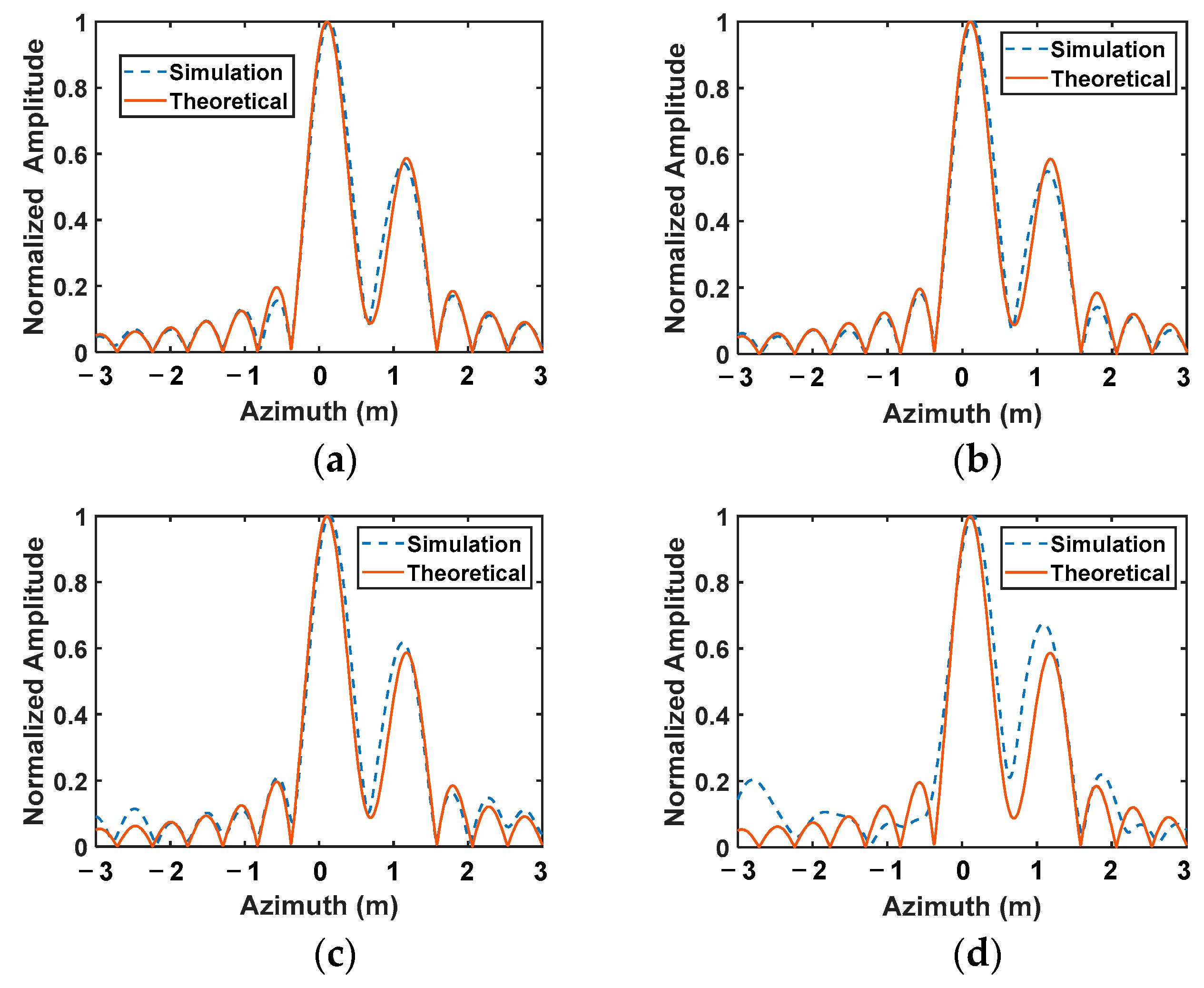
3.1. Verification of the BCA

As analyzed in Section 2.1, the BCA is utilized to capture the spatial correlation characteristics, serving as a fundamental approach for establishing the grid quantization criterion. The reconstructed image is the summation of correlation functions for multiple point targets based on the BCA. Remarkably, in radar systems, the noise from the radar receiver and clutter from the scene are primary sources of noise that have a significant impact on the imaging performance. Therefore, simulations of imaging under different SNRS are first carried out to verify the effectiveness of the BCA. In the simulation experiments, noise is equivalent to Gaussian White noise. The imaging scene of simulations is formed as depicted in Figure 1. Considering an MRCI system with a uniform linear array containing 21 transmitters and 1 receiver, the spacing of each transmitting element is 0.3 m. The other parameter settings of the system are listed in

Table 1. System simulation parameter settings.

Parameter (Variable Name)	Value
Imaging distance ($R$)	100 m
Carrier frequency ($f_c$)	10 GHz
Bandwidth	500 MHz
Pulse width ($T_p$)	100 μs
Sampling rate	1.5 GHz

. The imaging region contains three point targets, the azimuth positions of which are 0 m, 0.3 m, 1.1 m.

As depicted in Figure 12, when the SNR is 10 dB, 0 dB, and −10 dB, the simulation results are generally consistent with the theoretical results calculated in Equation (7); a slight deviation between them is observed when the SNR reaches −20 dB. Figure 13 illustrates the Root Mean Square Error (RMSE) with respect to the SNR, revealing that the RMSE remains below 0.1 when the SNR exceeds −25 dB. In summary, the BCA demonstrates superior robustness with respect to noise due to the low correlation property between noise and random radiation fields generated by the MRCI system.

In the MRCI system, the random radiation field generated by the random modulation of the transmitting signal is a critical factor impacting imaging performance. Adequate modulation can produce sufficient test modes with low correlation coefficients (CCs) [25]. However, achieving sufficient modulation is not always possible, resulting in higher CCs, especially when the radiation source is a random modulation metasurface aperture. As depicted in Figure 14, the normalized correlation function (NCF) weakens as the mean correlation coefficient (MCC) improves, particularly when the MCC exceeds 0.25.

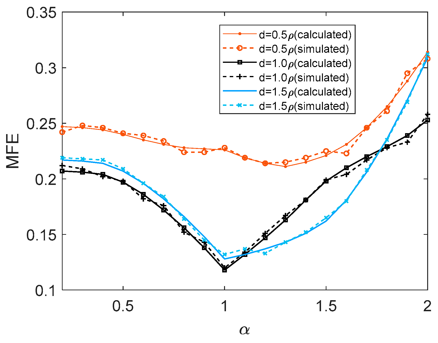
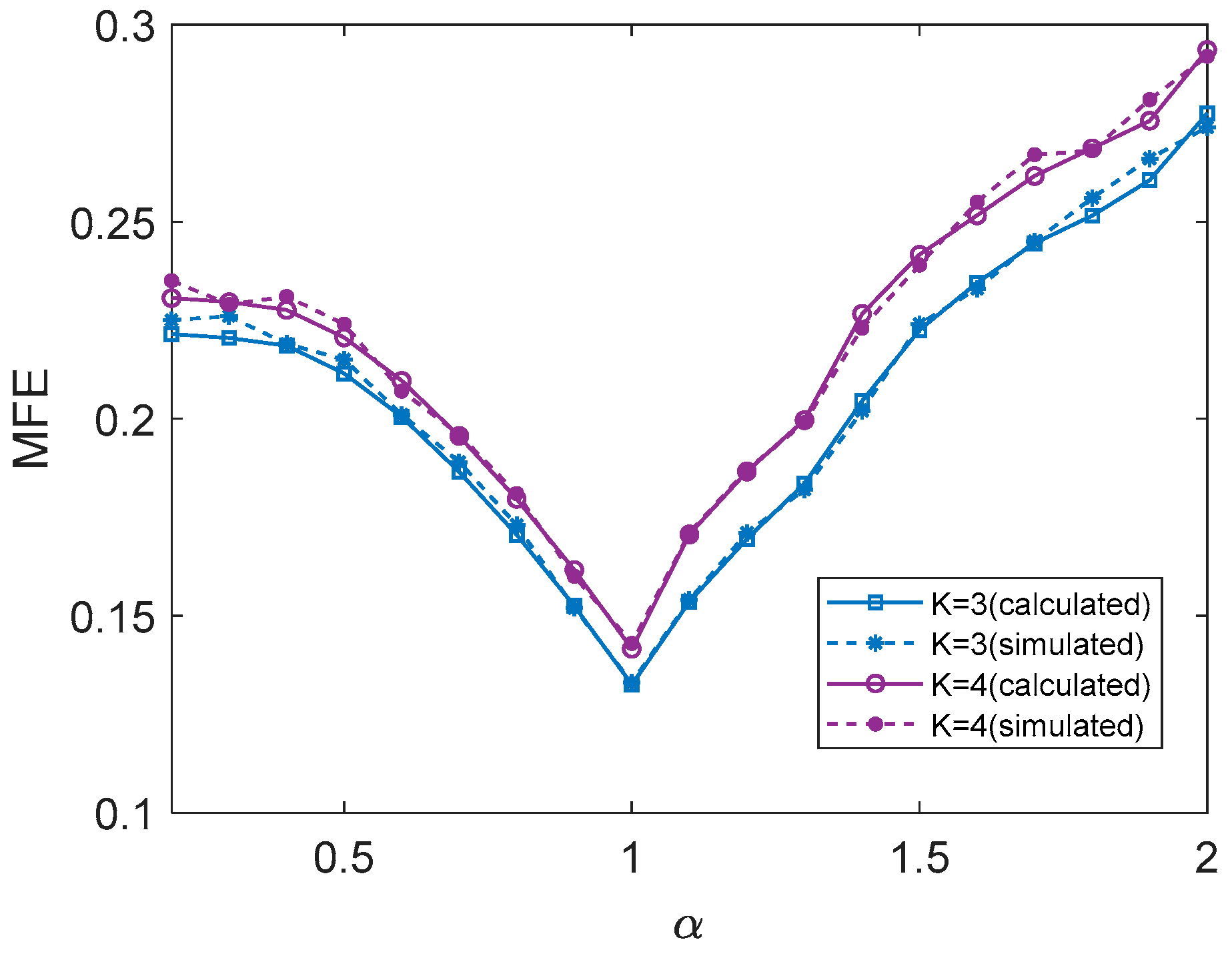
3.2. Verification of the Grid Quantization Criterion

In Section 2.2.2 and Section 2.2.3, the PDF of the imaging amplitude for a single point target and the MFE for multiple point targets are calculated. In this section, the results are analyzed through simulation.

The 3 dB main lobe of the correlation pattern regarded as one coherence length is about $\rho =0.5 \mathrm{m}$ for the MRCI system. The simulation results are the average performance of 10⁵ Monte Carlo experiments. The other parameters are consistent with the parameters in Section 3.1.

As shown in Figure 15, the MFE with respect to the GRR is simulated for one point target. The imaging region is 10 m (i.e., 20 times the coherence length), which remains constant. The number of the grid cell varies with the grid size. For one target, the simulation results are consistent with the calculation results in general. The MFE reaches its lowest when $\alpha =1$.

As shown in Figure 16, the distribution of imaging points is consistent with the targets analyzed in Section 2.2.3, and the simulated results are consistent with the calculated results in general. For two imaging points, the GRR of the lowest MFE remains 1 when the spacing of scattering points $d\ge \rho$. When $d<\rho$, the suitable GRR is greater than 1. As shown in Figure 17, Figure 18 and Figure 19, for multiple imaging points, the variation tendency of MFE with respect to the GRR is similar for different number of point targets. The GRR of the lowest MFE remains unchanged when $d$ is unchanged. The simulated results verify the analysis of the relationship between imaging performance and grid quantization, and the criterion of the grid quantization is valid.

4. Conclusions

To obtain a criterion of the grid quantization in the MRCI system, the performance of the MRCI system related to the grid size and the distribution of point targets was investigated in this paper. To evaluate the imaging performance with the off-grid problem in the MRCI, the imaging quality was expressed by statistical results as the point targets were considered to have an equal-probability distribution in the imaging area. Subsequently, we proposed the effective quantitative evaluations (the DP and the MFE) for the imaging performance with a single point target and multiple point targets. Therefore, the relationship between the grid quantization of the imaging area and the performance of the MRCI system was obtained under the BCM, which could provide the theoretical guidance for the grid quantization in the MRCI. The superior robustness of the BCM with respect to noise was investigated, ensuring the suitability of the grid quantization criterion for application. The validity of the analyses was verified through simulation experiments.

References

1. Ausherman, D.A.; Kozma, A.; Walker, J.L.; Jones, H.M.; Poggio, E.C. Developments in Radar Imaging. IEEE Trans. Aerosp. Electron. Syst. 1984, 20, 363–400. [Google Scholar] [CrossRef]
2. Wiley, C.A. Synthetic Aperture Radars. IEEE Trans. Aerosp. Electron. Syst. 1985, 21, 440–443. [Google Scholar] [CrossRef]
3. Xi, L.; Guosui, L.; Ni, J. Autofocusing of ISAR images based on entropy minimization. IEEE Trans. Aerosp. Electron. Syst. 1999, 35, 1240–1252. [Google Scholar] [CrossRef]
4. Zhang, R.; Cheng, L.; Zhang, W.; Guan, X.; Cai, Y.; Wu, W.; Zhang, R. Channel Estimation for Movable-Antenna MIMO Systems via Tensor Decomposition. IEEE Wirel. Commun. Lett. 2024. early access. [Google Scholar] [CrossRef]
5. Ma, Y.; Miao, C.; Long, W.; Zhang, R.; Chen, Q.; Zhang, J.; Wu, W. Time-Modulated Arrays in Scanning Mode Using Wideband Signals for Range-Doppler Estimation with Time-Frequency Filtering and Fusion. IEEE Trans. Aerosp. Electron. Syst. 2024, 60, 980–990. [Google Scholar] [CrossRef]
6. Hardy, N.D.; Shapiro, J.H. Ghost imaging in reflection: Resolution, contrast, and signal-to-noise ratio. Quantum Communications and Quantum Imaging VIII. Proc. SPIE 2010, 7815, 78150L. [Google Scholar]
7. Sun, B.; Welsh, S.; Edgar, M.P.; Shapiro, J.H.; Padgett, M. Normalized ghost imaging. Opt. Express 2012, 20, 16892–16901. [Google Scholar] [CrossRef]
8. Li, D.; Li, X.; Qin, Y.; Cheng, Y.; Wang, H. Radar Coincidence Imaging: An Instantaneous Imaging Technique with Stochastic Signals. IEEE Trans. Geosci. Remote Sens. 2014, 52, 2261–2277. [Google Scholar]
9. Zhu, S.; Zhang, A.; Xu, Z.; Dong, X. Radar Coincidence Imaging with Random Microwave Source. IEEE Antennas Wirel. Propag. Lett. 2015, 14, 1239–1242. [Google Scholar] [CrossRef]
10. Zhu, S.; He, Y.; Shi, H.; Zhang, A.; Xu, Z.; Dong, X. Mixed Mode Radar Coincidence Imaging with Hybrid Excitation Radar Array. IEEE Trans. Aerosp. Electron. Syst. 2018, 54, 1589–1604. [Google Scholar] [CrossRef]
11. Zhou, X.; Fan, B.; Wang, H.; Cheng, Y.; Qin, Y. Sparse Bayesian Perspective for Radar Coincidence Imaging with Array Position Error. IEEE Sens. J. 2017, 17, 5209–5219. [Google Scholar] [CrossRef]
12. Zhu, S.; He, Y.; Chen, X.; Guo, C.; Shi, H.; Li, J.; Dong, X.; Zhang, A. Resolution Threshold Analysis of the Microwave Radar Coincidence Imaging. IEEE Trans. Geosci. Remote Sens. 2020, 58, 2232–2243. [Google Scholar] [CrossRef]
13. Yuan, B.; Guo, Y.; Chen, W.; Wang, D. A Novel Microwave Staring Correlated Radar Imaging Method Based on Bi-Static Radar System. Sensors 2019, 19, 879. [Google Scholar] [CrossRef] [PubMed]
14. Li, R.; Luo, Y.; Zhang, Q.; Chen, Y.-J.; Wang, D. Radar Coincidence Imaging with a Uniform Circular Array. IEEE Access 2020, 8, 105226–105236. [Google Scholar] [CrossRef]
15. Li, D.; Li, X.; Cheng, Y.; Qin, Y.; Wang, H. Radar coincidence imaging in the presence of target-motion-induced error. J. Electron. Imag. 2014, 23, 023014. [Google Scholar] [CrossRef]
16. Zhou, X.; Wang, H.; Cheng, Y.; Qin, Y. Radar coincidence imaging with phase error using Bayesian hierarchical prior modeling. J. Electron. Imag. 2016, 25, 013018. [Google Scholar] [CrossRef]
17. Quan, Y.; Zhang, R.; Li, Y.; Xu, R.; Zhu, S.; Xing, M. Microwave Correlation Forward-Looking Super-Resolution Imaging Based on Compressed Sensing. IEEE Trans. Geosci. Remote Sens. 2021, 59, 8326–8337. [Google Scholar] [CrossRef]
18. Bai, X.; Wang, G.; Liu, S.; Zhou, F. High-Resolution Radar Imaging in Low SNR Environments Based on Expectation Propagation. IEEE Trans. Geosci. Remote Sens. 2021, 59, 1275–1284. [Google Scholar] [CrossRef]
19. Dai, F.; Zhang, S.; Li, L.; Liu, H. Enhancement of Metasurface Aperture Microwave Imaging via Information-Theoretic Waveform Optimization. IEEE Trans.Geosci. Remote Sens. 2022, 60, 1–12. [Google Scholar] [CrossRef]
20. Cao, K.; Cheng, Y.; Liu, K.; Wang, J.; Liu, H.; Wang, H. Reweighted-Dynamic-Grid-Based Microwave Coincidence Imaging with Grid Mismatch. IEEE Trans. Geosci. Remote Sens. 2021, 60, 1–10. [Google Scholar] [CrossRef]
21. Cao, K.; Cheng, Y.; Liu, K.; Wang, H.; Wang, J.; Liu, H. Off-Grid Microwave Coincidence Imaging Based on Directional Grid Fission. IEEE Antennas Wireless Propag. Lett. 2020, 19, 2497–2501. [Google Scholar] [CrossRef]
22. Cao, K.; Cheng, Y.; Liu, K.; Wang, J.; Wang, H. Coherent-Detecting and Incoherent-Modulating Microwave Coincidence Imaging with Off-Grid Errors. IEEE Geosci. Remote Sens. Lett. 2022, 19, 1–5. [Google Scholar] [CrossRef]
23. Dai, F.; Fu, H.; Hong, L.; Li, L.; Liu, H. Off-Grid Error and Amplitude–Phase Drift Calibration for Computational Microwave Imaging with Metasurface Aperture Based on Sparse Bayesian Learning. IEEE Trans. Geosci. Remote Sens. 2022, 60, 1–14. [Google Scholar] [CrossRef]
24. Zhao, M.; Zhang, J.; Li, A.; García-Fernández, M.; Álvarez-Narciandi, G.; Zhu, S.; Yurduseven, O. Microwave Computational Imaging-Based Near-Field Measurement Method. IEEE Antennas Wireless Propag. Lett. 2024; early access. [Google Scholar] [CrossRef]
25. Zhao, M.; Zhu, S.; Lynch, D.P.; Nian, Y.; Fromenteze, T.; Khalily, M.; Chen, X.; Fusco, V.; Yurduseven, O. Frequency-Diverse Metacavity Cassegrain Antenna for Differential Coincidence Imaging. IEEE Trans. Antennas Propag. 2023, 71, 9054–9059. [Google Scholar] [CrossRef]
Figure 1. Typical scene of MRCI.
Remotesensing 16 03726 g001
Figure 2. Imaging process using BCA.
Remotesensing 16 03726 g002
Figure 3. Schematic diagram of PDF of the imaging amplitude for one point target.
Remotesensing 16 03726 g003
Figure 4. Single point target. (a) Target expression result. (b) Imaging result; the grid offset ratio is −0.25.
Remotesensing 16 03726 g004
Figure 5. Two point targets. (a) Target expression result. (b) Imaging result; the grid offset ratio is −0.25 and −0.5.
Remotesensing 16 03726 g005
Figure 6. PDF of the imaging amplitude of one grid cell for one point target.
Remotesensing 16 03726 g006
Figure 7. The DP of a single point target.
Remotesensing 16 03726 g007
Figure 8. Flowchart for the derivation of PDF and DP.
Remotesensing 16 03726 g008
Figure 9. The MFE for one point target.
Remotesensing 16 03726 g009
Figure 10. MFE for two point targets with different spacing.
Remotesensing 16 03726 g010
Figure 11. MFE for different number of point targets, d = 1.0 ρ .
Remotesensing 16 03726 g011
Figure 12. The reconstructed image of simulation and theoretical under different SNRs (a) SNR = 10 dB (b) SNR = 0 dB (c) SNR = −10 dB (d) SNR = −20 dB.
Remotesensing 16 03726 g012
Figure 13. RMSE with respect to SNR.
Remotesensing 16 03726 g013
Figure 14. NCF with respect to MCC.
Remotesensing 16 03726 g014
Figure 15. MFE for a single point target (calculated and simulated results).
Remotesensing 16 03726 g015
Figure 16. MFE for two point targets with different spacing (calculated and simulated results).
Remotesensing 16 03726 g016
Figure 17. MFE for different number of point targets, d = 0.5 ρ (calculated and simulated results).
Remotesensing 16 03726 g017
Figure 18. MFE for different number of point targets, d = 1.0 ρ (calculated and simulated results).
Remotesensing 16 03726 g018
Figure 19. MFE for different number of point targets, d = 1.5 ρ (calculated and simulated results).
Remotesensing 16 03726 g019