

Semi-Supervised Subcategory Centroid Alignment-Based Scene Classification for High-Resolution Remote Sensing Images †


Abstract
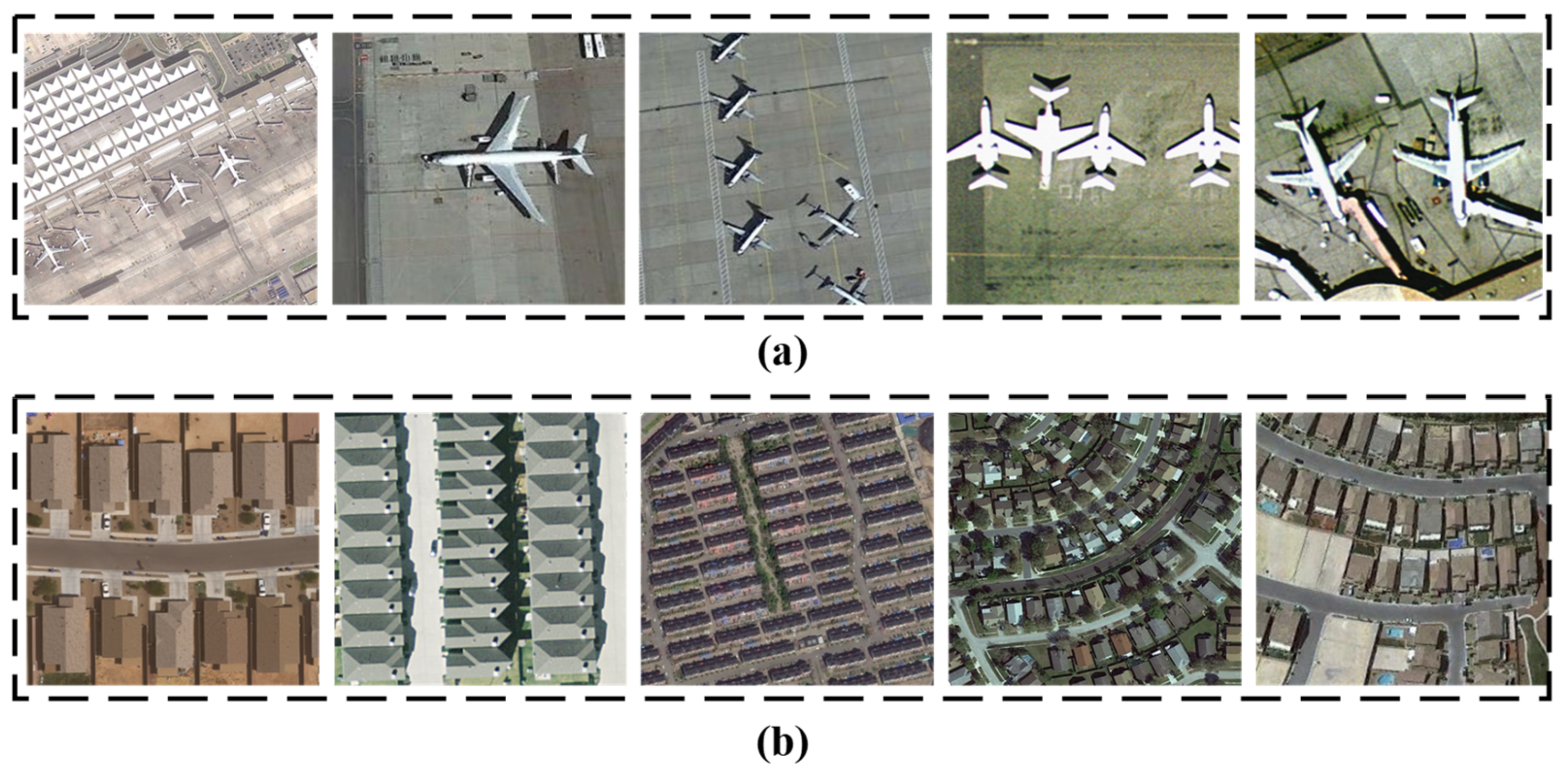
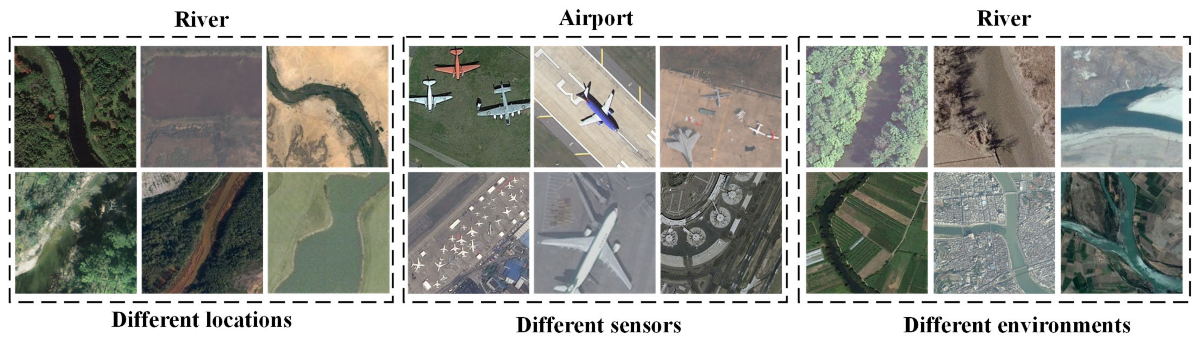
:1. Introduction
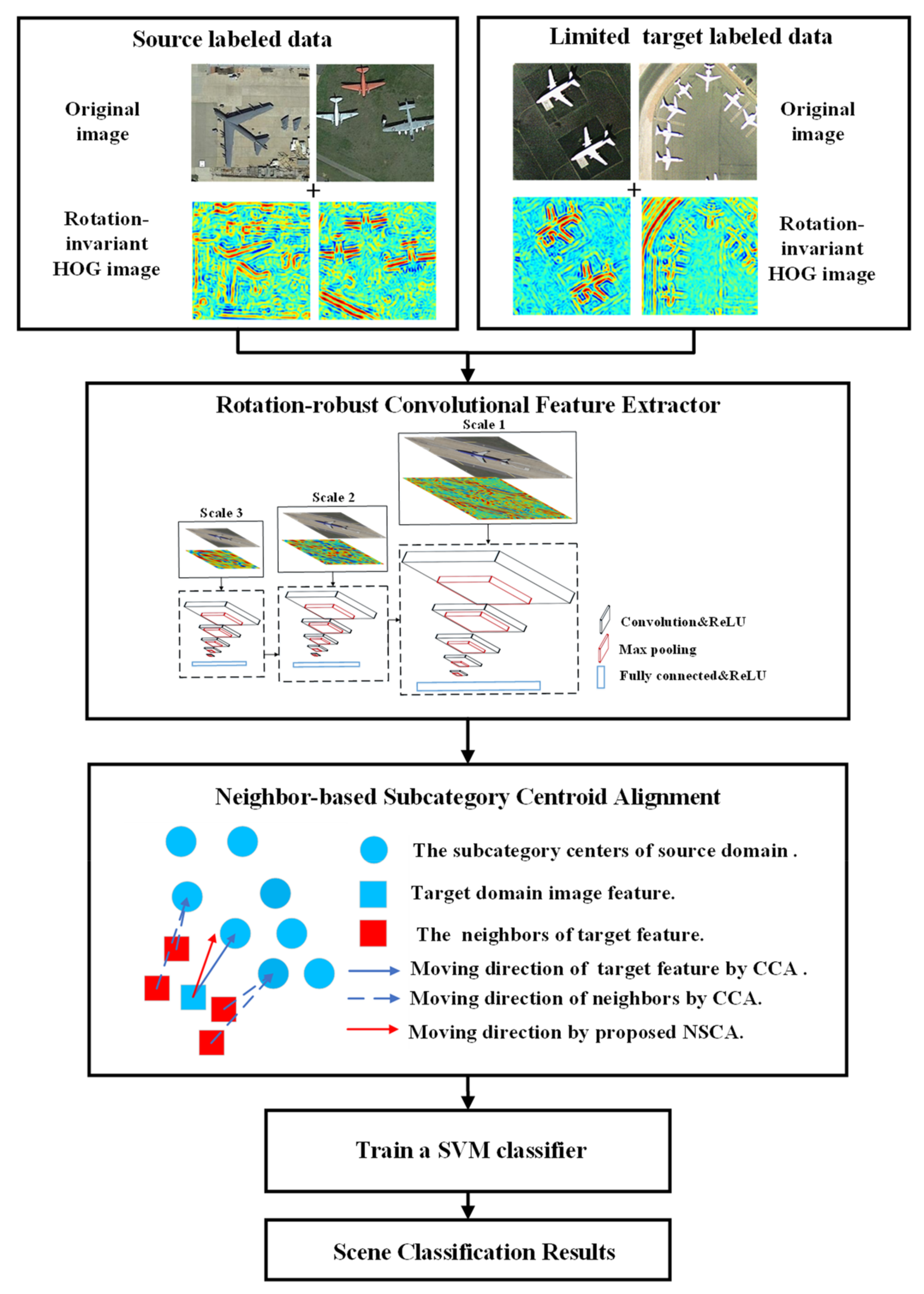
- The proposed RCFE incorporates rotation robustness into convolution feature extractor where both rotation-invariant HOG images and original images are considered as the input, which can reduce the impact of spectral shift and rotation variance on feature extraction.
- We proposed the NSCA method by moving the target features toward the relevant subcategories of their source domain features in order to reduce the deviation between feature distributions across domains.
- The proposed SSCA framework with RCFE and NSCA achieves a classification accuracy that is better than that of most of existing methods on two testing datasets.
2. Materials and Methods
2.1. Generating Rotation-Invariant HOG Images
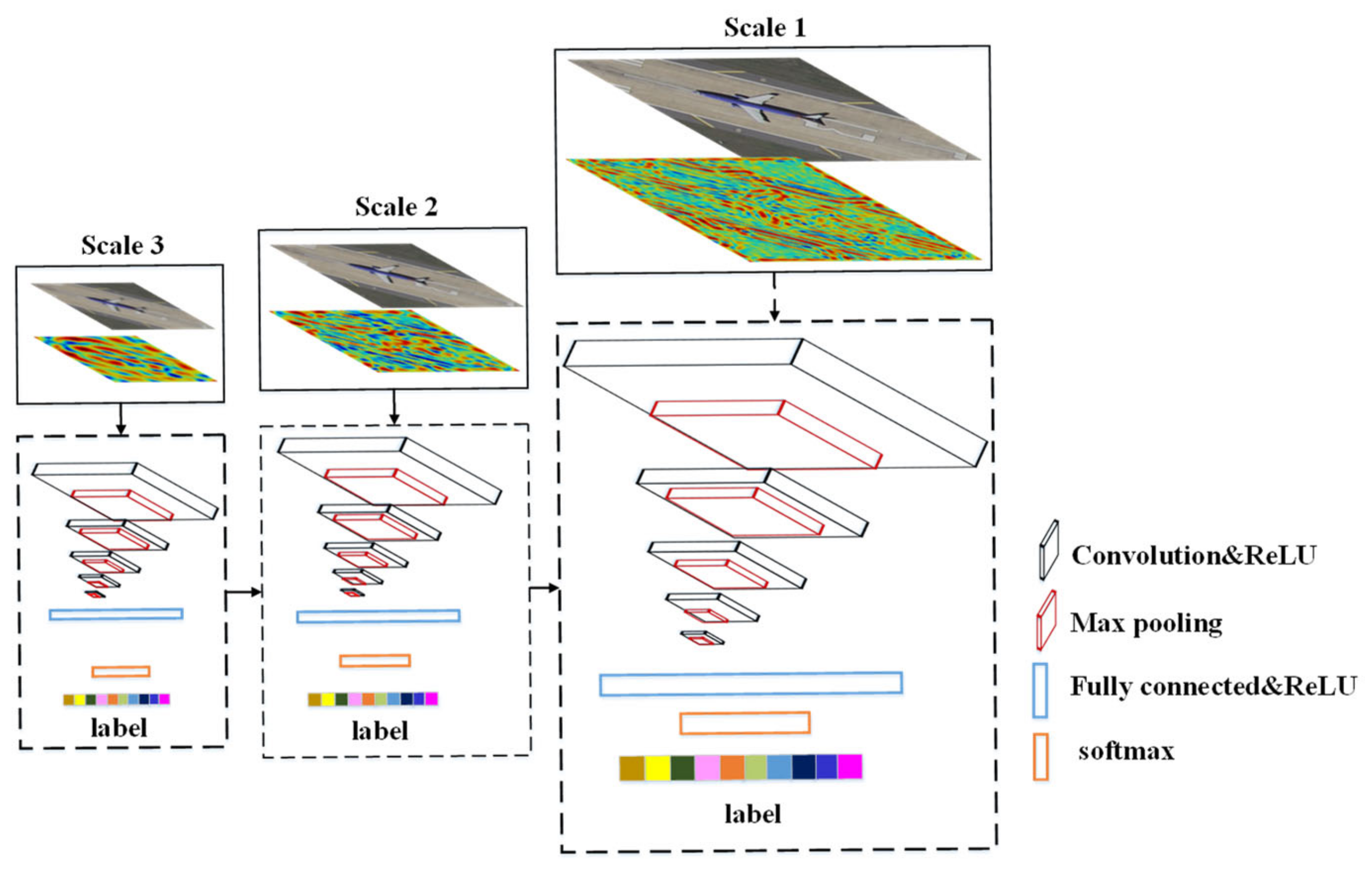
2.2. Rotation-Robust Convolutional Feature Extractor
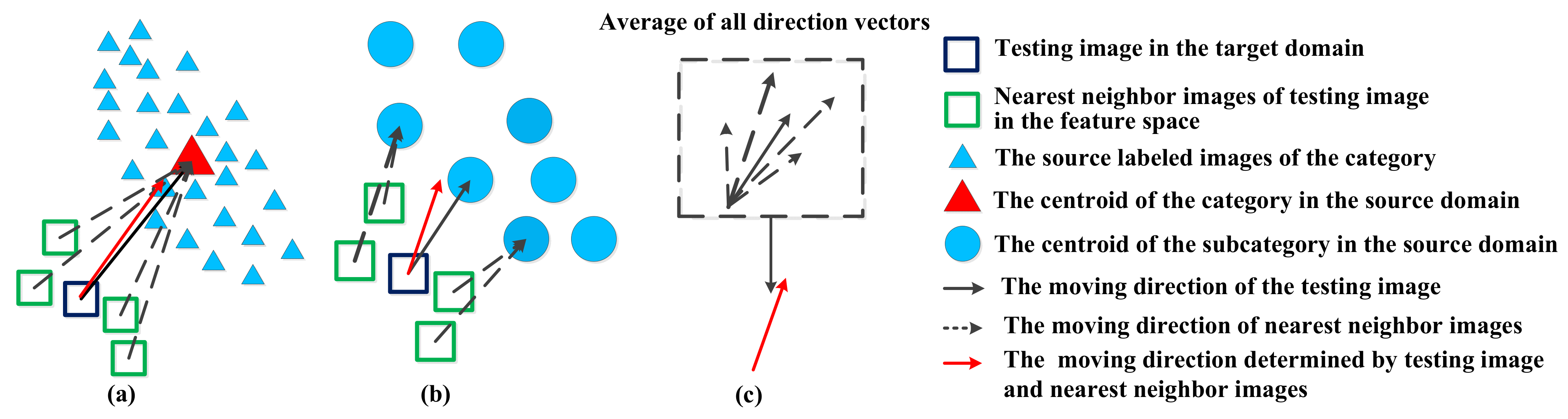
2.3. Neighbor-Based Subcategory Centroid Alignment
| Algorithm 1 NSCA approach description |
| 1: Input: target features , target labels , source features , source labels , category number C, nearest neighbor number M, subcategory number k. |
| 2: Output: target features after moving . |
| 3: Source features of all categories are divided into k × C subcategories with k-means. There exist k subcategories in each category, represent all subcategories. The source and target images belong to are considered as label . |
| 4: While predictions is not convergent do |
| 5: A classifier of k × C subcategories is trained based on , and . |
| 6: When the iteration l is set to 1, the predicted label for is predicted by the trained classifier. |
| 7: and is estimated based on and . |
| 8: is calculated for each subcategory based on Equations (6)–(8). |
| 9: Find M nearest neighbors for each target feature, whose direction is calculated by Equation (9). |
| 10: Each target feature is moved based on |
| 11: The moved target feature is predicted by the classifier in step 5. |
| 12. The predicted label is updated in the iteration l + 1 |
| 13: End while |
| 14: Return |
3. Results
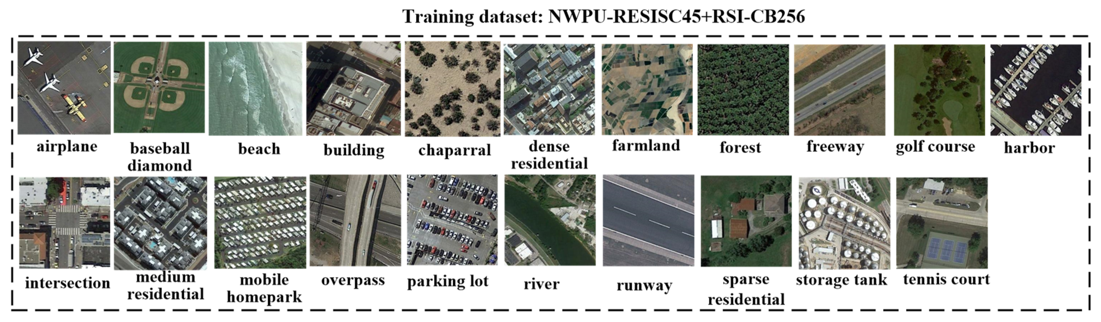
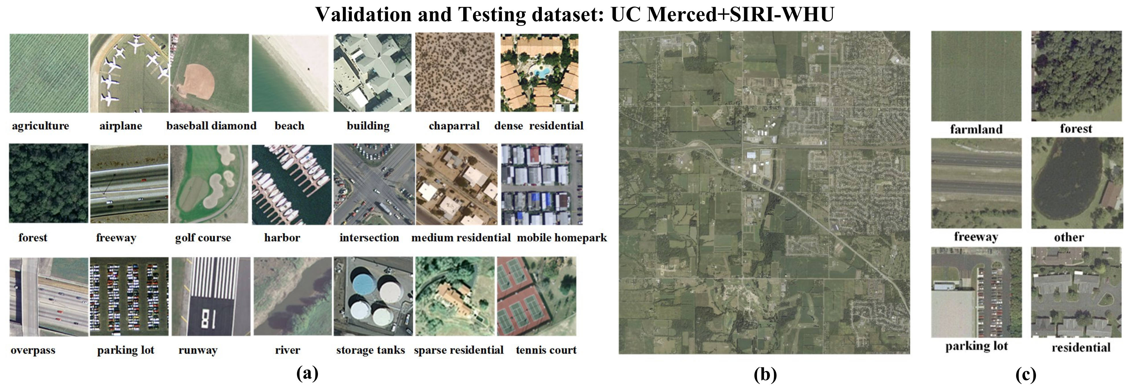
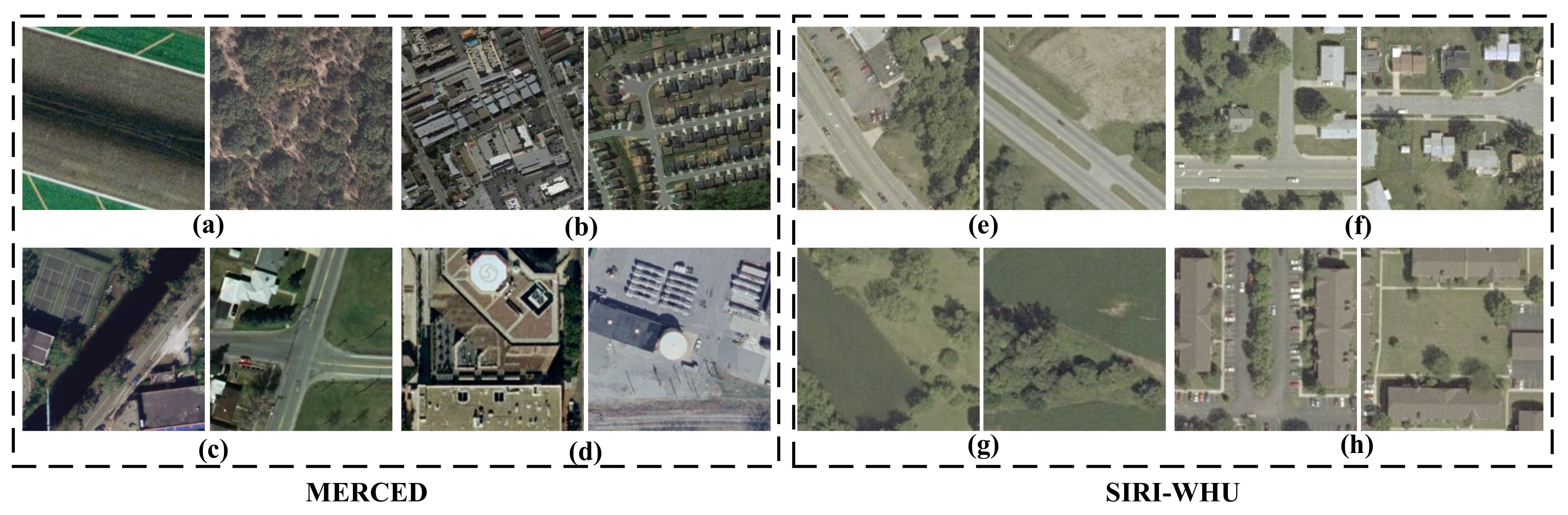
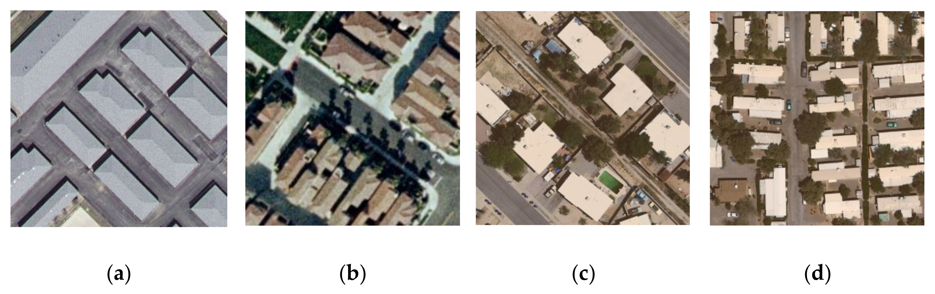
3.1. Dataset Partition and Description
3.2. Experimental Setup
3.3. Comparison Experiment
3.4. Ablation Experiment
4. Discussion
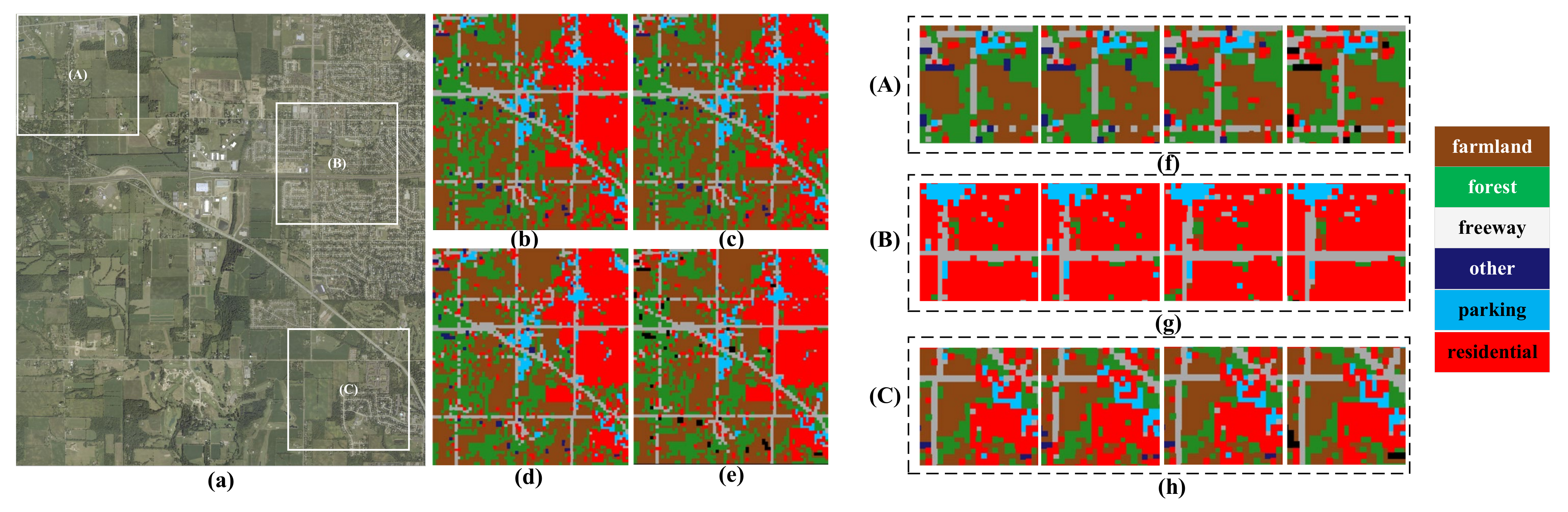
4.1. Confusion Analysis
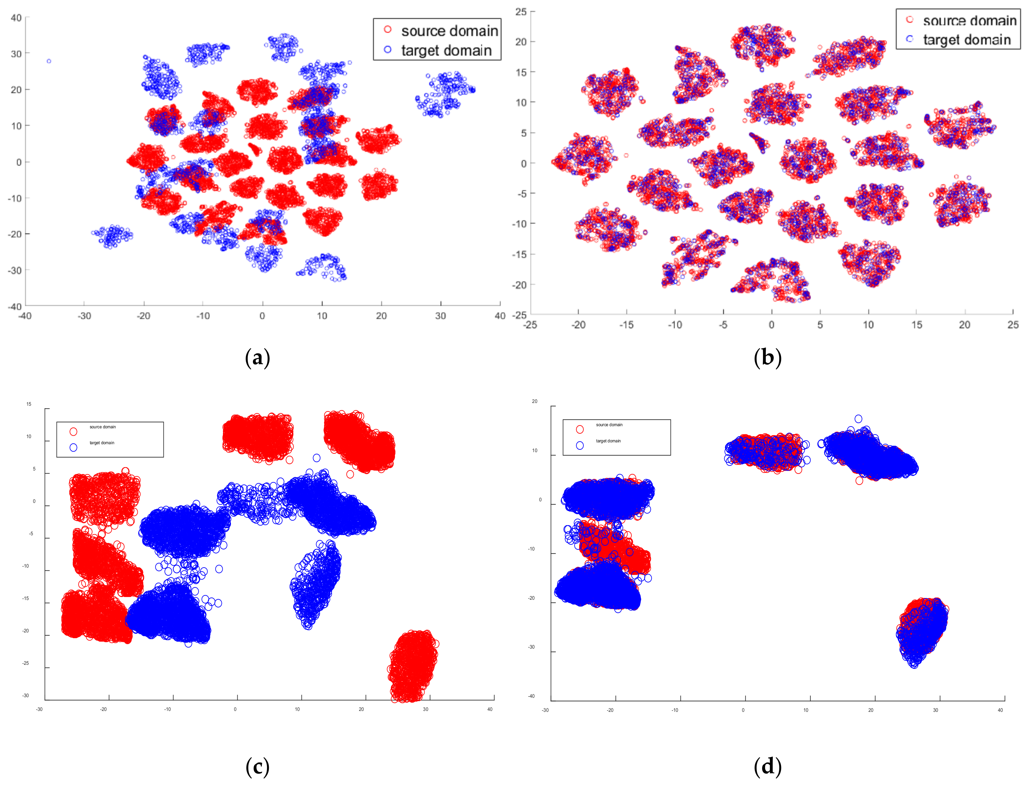
4.2. Feature Visualization
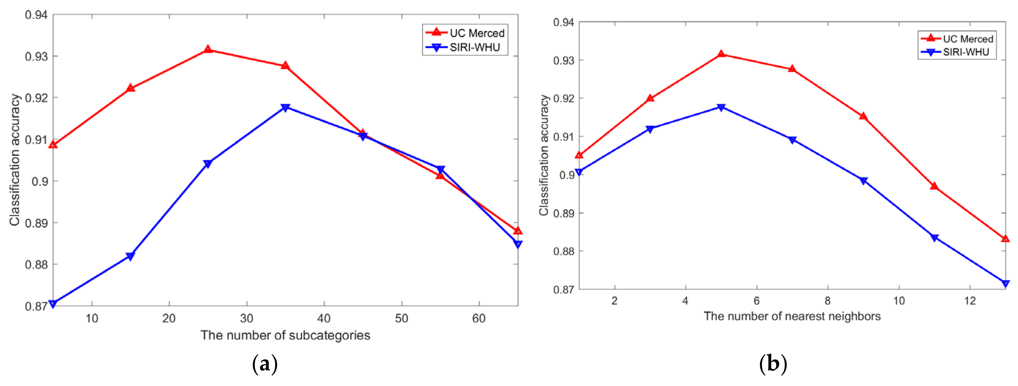
4.3. Sensitivity Analysis
5. Conclusions
Author Contributions
Funding
Data Availability Statement
Conflicts of Interest
References
- Cheng, G.; Xie, X.; Han, J.; Guo, L.; Xia, G.S. Remote sensing image scene classification meets deep learning: Challenges, methods, benchmarks, and opportunities. IEEE J. Sel. Top. Appl. Earth Obs. Remote Sens. 2020, 13, 3735–3756. [Google Scholar] [CrossRef]
- Adegun, A.A.; Viriri, S.; Tapamo, J.R. Review of deep learning methods for remote sensing satellite images classification: Experimental survey and comparative analysis. J. Big Data 2023, 10, 93. [Google Scholar] [CrossRef]
- Zhang, Q.; Yuan, Q.; Song, M.; Yu, H.; Zhang, L. Cooperated spectral low-rankness prior and deep spatial prior for HSI unsupervised denoising. IEEE Trans. Image Process. 2022, 31, 6356–6368. [Google Scholar] [CrossRef] [PubMed]
- Zhang, Q.; Zheng, Y.; Yuan, Q.; Song, M.; Yu, H.; Xiao, Y. Hyperspectral image denoising: From model-driven, data-driven, to model-data-driven. IEEE Trans. Neural Netw. Learn. Syst. 2023, 6, 1–21. [Google Scholar] [CrossRef] [PubMed]
- Thapa, A.; Horanont, T.; Neupane, B.; Aryal, J. Deep learning for remote sensing image scene classification: A review and meta-analysis. Remote Sens. 2023, 15, 4804. [Google Scholar] [CrossRef]
- Qiao, H.; Qian, W.; Hu, H.; Huang, X.; Li, J. Semi-Supervised Building Extraction with Optical Flow Correction Based on Satellite Video Data in a Tsunami-Induced Disaster Scene. Sensors 2024, 24, 5205. [Google Scholar] [CrossRef]
- Liu, K.; Yang, J.; Li, S. Remote-Sensing Cross-Domain Scene Classification: A Dataset and Benchmark. Remote Sens. 2022, 14, 4635. [Google Scholar] [CrossRef]
- Tuia, D.; Persello, C.; Bruzzone, L. Domain Adaptation for the Classification of Remote Sensing Data: An Overview of Recent Advances. IEEE Geosci. Remote Sens. Mag. 2016, 4, 41–57. [Google Scholar] [CrossRef]
- Yan, L.; Zhu, R.; Mo, N.; Liu, Y. Cross-Domain Distance Metric Learning Framework with Limited Target Samples for Scene Classification of Aerial Images. IEEE Trans. Geosci. Remote Sens. 2019, 57, 3840–3857. [Google Scholar] [CrossRef]
- Yang, C.; Dong, Y.; Du, B.; Zhang, L. Attention-Based Dynamic Alignment and Dynamic Distribution Adaptation for Remote Sensing Cross-Domain Scene Classification. IEEE Trans. Geosci. Remote Sens. 2022, 60, 5634713. [Google Scholar] [CrossRef]
- Li, Y.; Li, Z.; Su, A.; Wang, K.; Wang, Z.; Yu, Q. Semi supervised Cross-Domain Remote Sensing Scene Classification via Category-Level Feature Alignment Network. IEEE Trans. Geosci. Remote Sens. 2024, 62, 5621614. [Google Scholar]
- Bahirat, K.; Bovolo, F.; Bruzzone, L.; Chaudhuri, S. A Novel Domain Adaptation Bayesian Classifier for Updating Land-Cover Maps with Class Differences in Source and Target Domains. IEEE Trans. Geosci. Remote Sens. 2012, 50, 2810–2826. [Google Scholar] [CrossRef]
- Wei, H.; Ma, L.; Liu, Y.; Du, Q. Combining Multiple Classifiers for Domain Adaptation of Remote Sensing Image Classification. IEEE J. Sel. Top. Appl. Earth Obs. Remote Sens. 2021, 14, 1832–1847. [Google Scholar] [CrossRef]
- Zheng, Z.; Zhong, Y.; Su, Y.; Ma, A. Domain Adaptation via a Task-Specific Classifier Framework for Remote Sensing Cross-Scene Classification. IEEE Trans. Geosci. Remote Sens. 2022, 60, 5620513. [Google Scholar] [CrossRef]
- Zhu, R.; Yan, L.; Mo, N.; Liu, Y. Semi-supervised center-based discriminative adversarial learning for cross-domain scene-level land-cover classification of aerial images. ISPRS J. Photogramm. Remote Sens. 2019, 155, 72–89. [Google Scholar] [CrossRef]
- Zhao, X.; Zhang, M.; Tao, R.; Li, W.; Liao, W.; Philips, W. Cross-Domain Classification of Multisource Remote Sensing Data Using Fractional Fusion and Spatial-Spectral Domain Adaptation. IEEE J. Sel. Top. Appl. Earth Obs. Remote Sens. 2022, 15, 5721–5733. [Google Scholar] [CrossRef]
- Zhu, S.; Wu, C.; Du, B.; Zhang, L. Style and content separation network for remote sensing image cross-scene generalization. ISPRS J. Photogramm. Remote Sens. 2023, 201, 1–11. [Google Scholar] [CrossRef]
- Ye, M.; Qian, Y.; Zhou, J.; Yuan, Y. Dictionary Learning-Based Feature-Level Domain Adaptation for Cross-Scene Hyperspectral Image Classification. IEEE Trans. Geosci. Remote Sens. 2017, 55, 1544–1562. [Google Scholar] [CrossRef]
- Patel, V.M.; Gopalan, R.; Li, R. Visual Domain Adaptation: An Overview of Recent Advances. IEEE Signal Process. Mag. 2015, 32, 53–69. [Google Scholar] [CrossRef]
- Tuia, D.; Volpi, M.; Trolliet, M.; Camps-Valls, G. Semi-supervised Manifold Alignment of Multimodal Remote Sensing Images. IEEE Trans. Geosci. Remote Sens. 2014, 52, 7708–7720. [Google Scholar] [CrossRef]
- Matasci, G.; Volpi, M.; Kanevski, M.; Bruzzone, L.; Tuia, D. Semisupervised Transfer Component Analysis for Domain Adaptation in Remote Sensing Image Classification. IEEE Trans. Geosci. Remote Sens. 2015, 53, 3550–3564. [Google Scholar] [CrossRef]
- Zhu, L.; Ma, L. Class centroid alignment based domain adaptation for classification of remote sensing images. Pattern Recognit. Lett. 2016, 83, 124–132. [Google Scholar] [CrossRef]
- Ojala, T.; Pietikäinen, M.; Mäenpää, T. Gray Scale and Rotation Invariant Texture Classification with Local Binary Patterns. IEEE Trans. Pattern Anal. Mach. Intell. 2002, 24, 971–987. [Google Scholar] [CrossRef]
- Skibbe, H.; Reisert, M. Circular Fourier-HOG features for rotation invariant object detection in biomedical images. In Proceedings of the IEEE International Symposium on Biomedical Imaging, Barcelona, Spain, 2–5 May 2012; pp. 450–453. [Google Scholar]
- Liu, K.; Skibbe, H.; Schmidt, T.; Blein, T.; Palme, K.; Brox, T.; Ronneberger, O. Rotation-Invariant HOG Descriptors Using Fourier Analysis in Polar and Spherical Coordinates. Int. J. Comput. Vis. 2014, 106, 342–364. [Google Scholar] [CrossRef]
- Gong, C.; Yang, C.; Yao, X.; Lei, G.; Han, J. When Deep Learning Meets Metric Learning: Remote Sensing Image Scene Classification via Learning Discriminative CNNs. IEEE Trans. Geosci. Remote Sens. 2018, 56, 2811–2821. [Google Scholar] [CrossRef]
- Jaderberg, M.; Simonyan, K.; Zisserman, A. Spatial transformer networks. In Proceedings of the Advances in Neural Information Processing Systems, Montreal, QC, Canada, 7–12 December 2015; pp. 2017–2025. [Google Scholar]
- Laptev, D.; Savinov, N.; Buhmann, J.M.; Pollefeys, M. TI-Pooling: Transformation-invariant pooling for feature learning in Convolutional Neural Networks. In Proceedings of the Computer Vision and Pattern Recognition, Las Vegas, NV, USA, 27–30 June 2016; pp. 289–297. [Google Scholar]
- Zhou, Y.; Ye, Q.; Qiang, Q.; Jiao, J. Oriented Response Networks. In Proceedings of the IEEE Conference on Computer Vision and Pattern Recognition, Honolulu, HI, USA, 21–26 July 2017; pp. 4961–4970. [Google Scholar]
- Cohen, T.S.; Welling, M. Group Equivariant Convolutional Networks. In Proceedings of the International Conference on Machine Learning, New York City, NY, USA, 19–24 June 2016; pp. 2990–2999. [Google Scholar]
- Marcos, D.; Volpi, M.; Kellenberger, B.; Tuia, D. Land cover mapping at very high resolution with rotation equivariant CNNs: Towards small yet accurate models. ISPRS J. Photogramm. Remote Sens. 2018, 145, 96–107. [Google Scholar] [CrossRef]
- Volpi, M.; Camps-Valls, G.; Tuia, D. Spectral alignment of multi-temporal cross-sensor images with automated kernel canonical correlation analysis. J. Photogram. Remote Sens. 2015, 107, 50–63. [Google Scholar] [CrossRef]
- Li, X.; Zhang, L.; Du, B.; Zhang, L.; Shi, Q. Iterative reweighting heterogeneous transfer learning framework for supervised remote sensing image classification. IEEE J. Sel. Topics Appl. Earth Observ. Remote Sens. 2017, 10, 2022–2035. [Google Scholar] [CrossRef]
- Sun, H.; Liu, S.; Zhou, S.; Zou, H. Transfer sparse subspace analysis for unsupervised cross-view scene model adaptation. IEEE J. Sel. Topics Appl. Earth Observ. Remote Sens. 2016, 9, 2901–2909. [Google Scholar] [CrossRef]
- He, K.; Zhang, X.; Ren, S.; Sun, J. Deep Residual Learning for Image Recognition. In Proceedings of the IEEE Conference on Computer Vision and Pattern Recognition, Las Vegas, NV, USA, 27–30 June 2016; pp. 770–778. [Google Scholar]
- Gong, C.; Han, J.; Lu, X. Remote Sensing Image Scene Classification: Benchmark and State of the Art. Proc. IEEE 2017, 105, 1865–1883. [Google Scholar]
- Li, H.; Dou, X.; Tao, C.; Wu, Z.; Chen, J.; Peng, J.; Deng, M.; Zhao, L. RSI-CB: A Large-Scale Remote Sensing Image Classification Benchmark Using Crowdsourced Data. Sensors 2020, 20, 1594. [Google Scholar] [CrossRef] [PubMed]
- Yi, Y.; Newsam, S. Bag-of-visual-words and spatial extensions for land-use classification. In Proceedings of the Sigspatial International Conference on Advances in Geographic Information Systems, San Jose, CA, USA, 2–5 November 2010; pp. 270–279. [Google Scholar]
- Zhong, Y.; Zhu, Q.; Zhang, L. Scene Classification Based on the Multifeature Fusion Probabilistic Topic Model for High Spatial Resolution Remote Sensing Imagery. IEEE Trans. Geosci. Remote Sens. 2015, 53, 6207–6222. [Google Scholar] [CrossRef]
- Qiang, Q.; Patel, V.M.; Turaga, P.; Chellappa, R. Domain Adaptive Dictionary Learning. In Proceedings of the European Conference on Computer Vision, Florence, Italy, 7–13 October 2012; pp. 631–645. [Google Scholar]
- Lu, B.; Chellappa, R.; Nasrabadi, N.M. Incremental Dictionary Learning for Unsupervised Domain Adaptation. In Proceedings of the British Machine Vision Conference, Swansea, UK, 7–10 September 2015; pp. 108.1–108.12. [Google Scholar]
- Ammour, N.; Bashmal, L.; Bazi, Y.; Rahhal, M.A.; Zuair, M. Asymmetric Adaptation of Deep Features for Cross-Domain Classification in Remote Sensing Imagery. IEEE Geosci. Remote Sens. Lett. 2018, 15, 597–601. [Google Scholar] [CrossRef]
- Tzeng, E.; Hoffman, J.; Saenko, K.; Darrell, T. Adversarial discriminative domain adaptation. In Proceedings of the IEEE Conference on Computer Vision and Pattern Recognition, Honolulu, HI, USA, 21–26 July 2017; pp. 7167–7176. [Google Scholar]
- Long, M.; Cao, Z.; Wang, J.; Jordan, M.I. Conditional adversarial domain adaptation. In Proceedings of the Advances in Neural Information Processing Systems, Montréal, QC, Canada, 3–8 December 2018; pp. 1640–1650. [Google Scholar]
- Zhang, W.; Ouyang, W.; Li, W.; Xu, D. Collaborative and adversarial network for unsupervised domain adaptation. In Proceedings of the IEEE Conference on Computer Vision and Pattern Recognition, Salt Lake City, UT, USA, 18–22 June 2018; pp. 3801–3809. [Google Scholar]
- AlRahhal, M.; Bazi, Y.; AlHichri, H.; Alajlan, N.; Melgani, F.; Yager, R.R. Deep learning approach for active classification of electrocardiogram signals. Inf. Sci. 2016, 345, 340–354. [Google Scholar]
- Ganin, Y.; Ustinova, E.; Ajakan, H.; Germain, P.; Larochelle, H.; Laviolette, F.; Marchand, M.; Lempitsky, V. Domain-adversarial training of neural networks. J. Mach. Learn. Res. 2016, 17, 1–35. [Google Scholar]


| Class | Training Dataset | Validation Dataset | Testing Dataset | |||
|---|---|---|---|---|---|---|
| NWPU-RESISC45 | RSI-CB256 | UC Merced | SIRI-WHU | UC Merced | SIRI-WHU | |
| airport | 700 | 351 | 20 | ✕ | 80 | ✕ |
| baseball | 700 | ✕ | 20 | ✕ | 80 | ✕ |
| beach | 700 | ✕ | 20 | ✕ | 80 | ✕ |
| buildings | ✕ | 1014 | 20 | ✕ | 80 | ✕ |
| chaparral | 700 | ✕ | 20 | ✕ | 80 | ✕ |
| dense residential | 700 | ✕ | 20 | ✕ | 80 | ✕ |
| farmland | 700 | 644 | 20 | 512 | 80 | 1549 |
| forest | 700 | 1082 | 20 | 286 | 80 | 1148 |
| freeway | 700 | 223 | 20 | 105 | 80 | 420 |
| golf course | 700 | ✕ | 20 | ✕ | 80 | ✕ |
| harbor | 700 | ✕ | 20 | ✕ | 80 | ✕ |
| intersection | 700 | ✕ | 20 | ✕ | 80 | ✕ |
| medium residential | 700 | ✕ | 20 | 271 | 80 | 1084 |
| mobile homepark | 700 | ✕ | 20 | ✕ | 80 | ✕ |
| overpass | 700 | ✕ | 20 | ✕ | 80 | ✕ |
| parking lot | 700 | 467 | 20 | 45 | 80 | 182 |
| river | 700 | 539 | 20 | 13 | 80 | 52 |
| runway | 700 | ✕ | 20 | ✕ | 80 | ✕ |
| sparse | 700 | ✕ | 20 | ✕ | 80 | ✕ |
| storage tank | 700 | 1307 | 20 | ✕ | 80 | ✕ |
| tennis court | 700 | ✕ | 20 | ✕ | 80 | ✕ |
| Types of Methods | Methods | Experimental Parameter Settings |
|---|---|---|
| Data distribution adaptation methods | SSCA | for UC Merced dataset; for SIRI-WHU dataset. |
| DADL | Sparsity level T = 0.4, tradeoff parameter , the codebook size s = 1300, the stopping threshold 0.9. | |
| IDL | The tradeoff parameter and normalization parameter , the codebook size s = 1300, and the number of supportive samples Q = 50. | |
| CCA | Number of the nearest neighbors , the parameters of SVM are the same as those in SSCA. | |
| AADF | 256-dimension features by DAE network in [46], dropout value is 0.5, learning rate is 0.1, momentum is 0.5, regularization parameter is 0.5, batch sizes are [100, 80, 60, 40, 20, 10]. | |
| Adversarial domain adaptation methods | SCDAL | . |
| CADA | Batch size 128; learning rate and momentum are the same as in the domain adversarial neural network (DANN) [47]. | |
| CAN | The initial learning rate is 0.0015, which is decreased gradually after each iteration, as in DANN. The weight decay, momentum, and batch size were 3 × 10⁻⁴, 0.9, and 128. | |
| ADDA | Batch size is 128, maximum iterations are 20,000, and learning rate is 1 × 10⁻⁴. |
| Method | UC Merced | SIRI-WHU |
|---|---|---|
| The proposed SSCA | 0.9314 | 0.9177 |
| SCDAL | 0.9118 | 0.8958 |
| ADDA | 0.8723 | 0.8617 |
| CADA | 0.8938 | 0.8850 |
| CAN | 0.8972 | 0.8756 |
| DADL | 0.8670 | 0.8425 |
| IDL | 0.8625 | 0.8541 |
| CCA | 0.8528 | 0.8478 |
| AADF | 0.8981 | 0.8730 |
| Method | UC Merced | SIRI-WHU |
|---|---|---|
| The proposed SSCA framework | 0.9314 | 0.9177 |
| Without rotation-invariant HOG | 0.9119 | 0.9043 |
| Without the NSCA method | 0.8933 | 0.8748 |
Disclaimer/Publisher’s Note: The statements, opinions and data contained in all publications are solely those of the individual author(s) and contributor(s) and not of MDPI and/or the editor(s). MDPI and/or the editor(s) disclaim responsibility for any injury to people or property resulting from any ideas, methods, instructions or products referred to in the content. |
© 2024 by the authors. Licensee MDPI, Basel, Switzerland. This article is an open access article distributed under the terms and conditions of the Creative Commons Attribution (CC BY) license (https://creativecommons.org/licenses/by/4.0/).
Share and Cite
Mo, N.; Zhu, R. Semi-Supervised Subcategory Centroid Alignment-Based Scene Classification for High-Resolution Remote Sensing Images. Remote Sens. 2024, 16, 3728. https://doi.org/10.3390/rs16193728
Mo N, Zhu R. Semi-Supervised Subcategory Centroid Alignment-Based Scene Classification for High-Resolution Remote Sensing Images. Remote Sensing. 2024; 16(19):3728. https://doi.org/10.3390/rs16193728
Chicago/Turabian StyleMo, Nan, and Ruixi Zhu. 2024. "Semi-Supervised Subcategory Centroid Alignment-Based Scene Classification for High-Resolution Remote Sensing Images" Remote Sensing 16, no. 19: 3728. https://doi.org/10.3390/rs16193728