A New NDSA (Normalized Differential Spectral Attenuation) Measurement Campaign for Estimating Water Vapor along a Radio Link

 , , , , , and
Abstract
:1. Introduction
2. Materials and Methods
2.1. The NDSA Approach: Spectral Sensitivity and IWV
2.2. The SWAMM-2 Instrument for Spectral Sensitivity Measurements
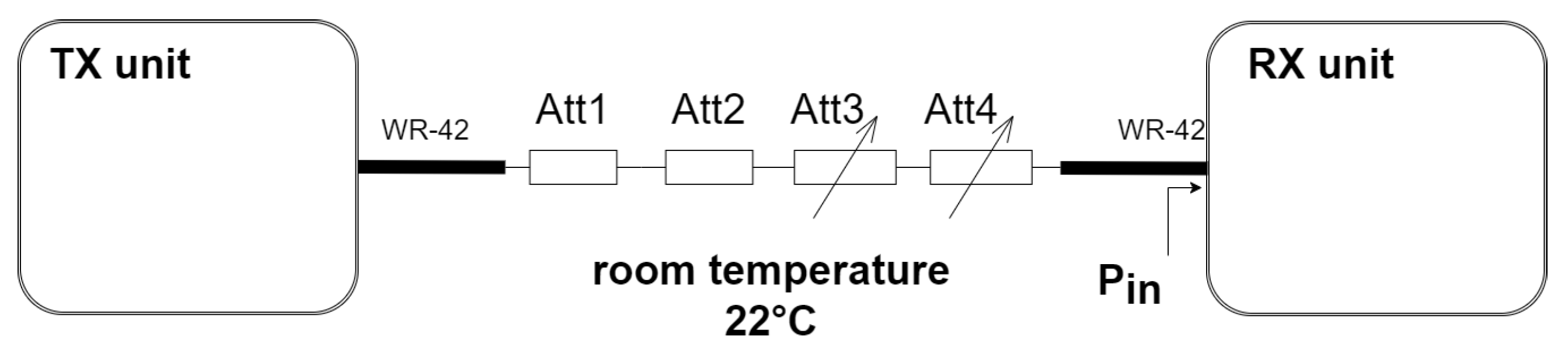
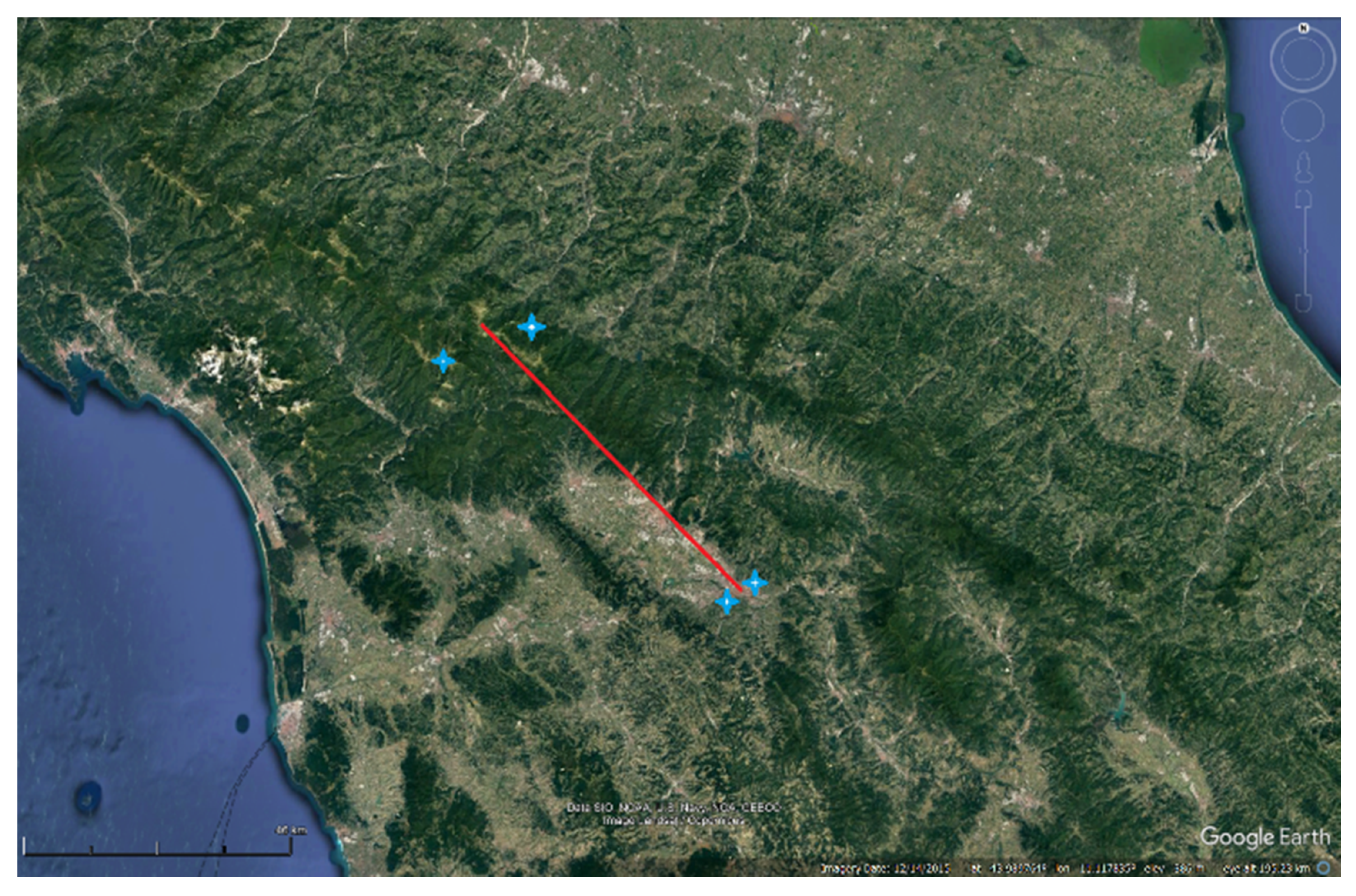
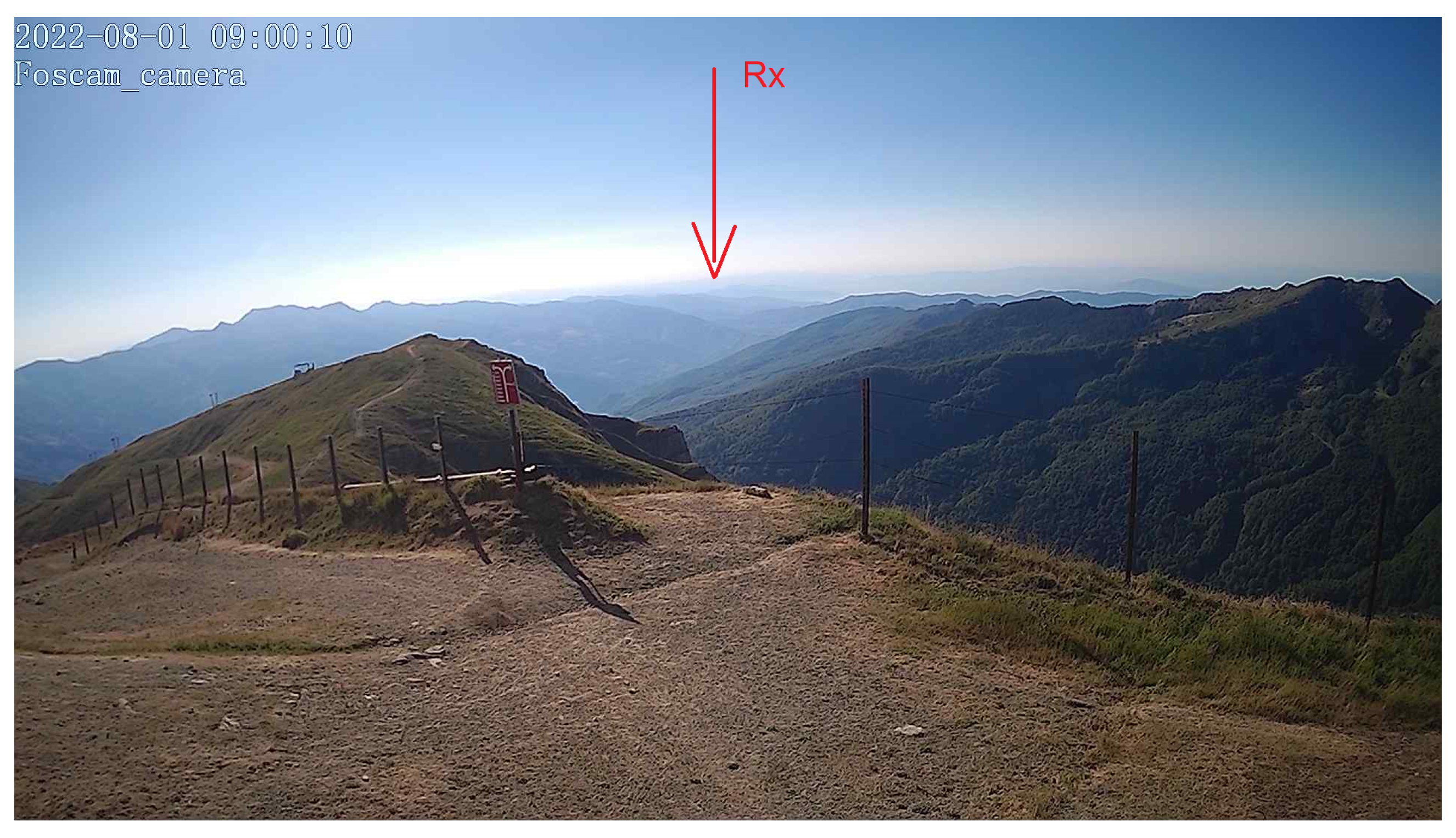
2.3. Measurement Setup and Campaign
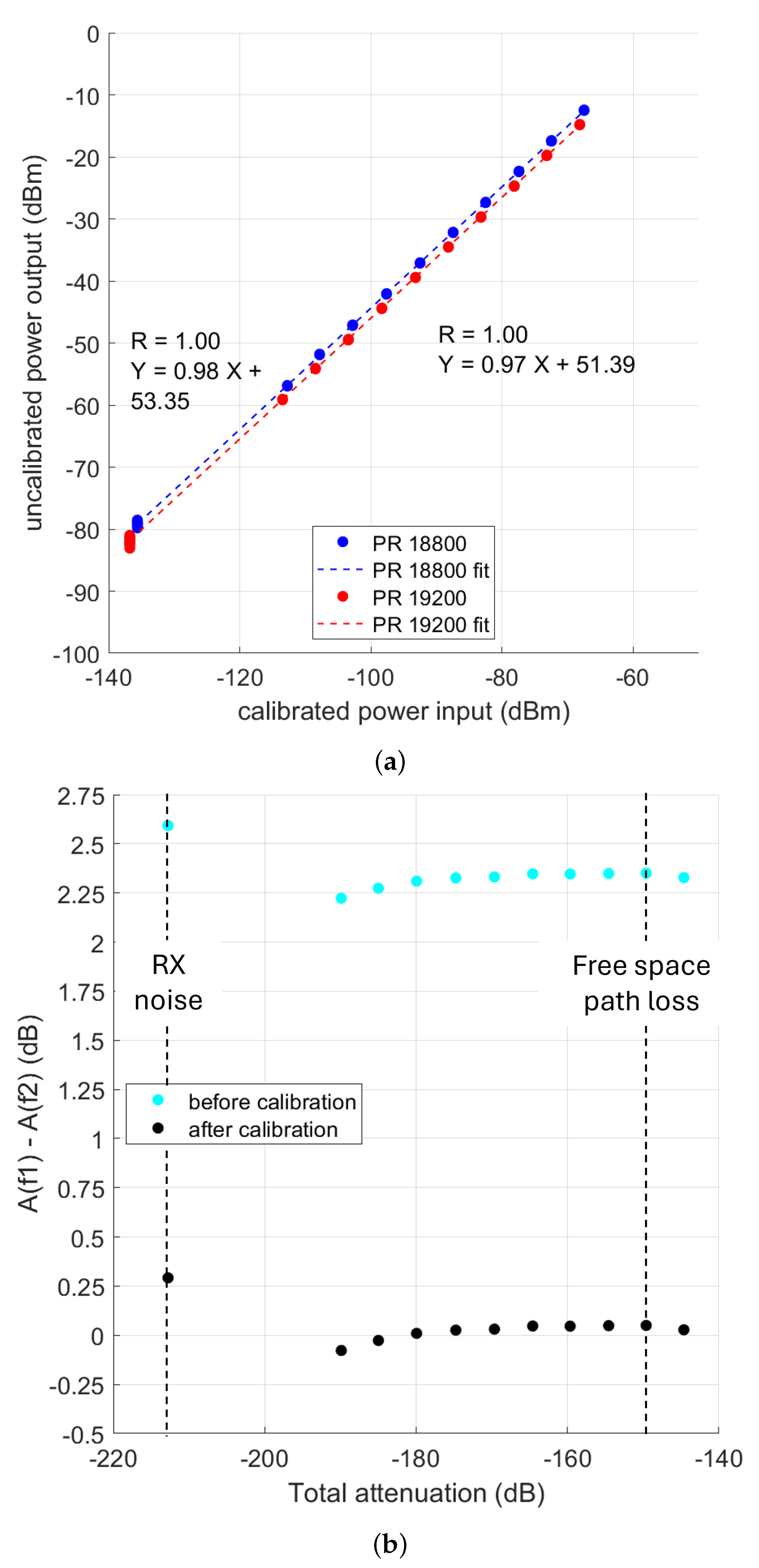
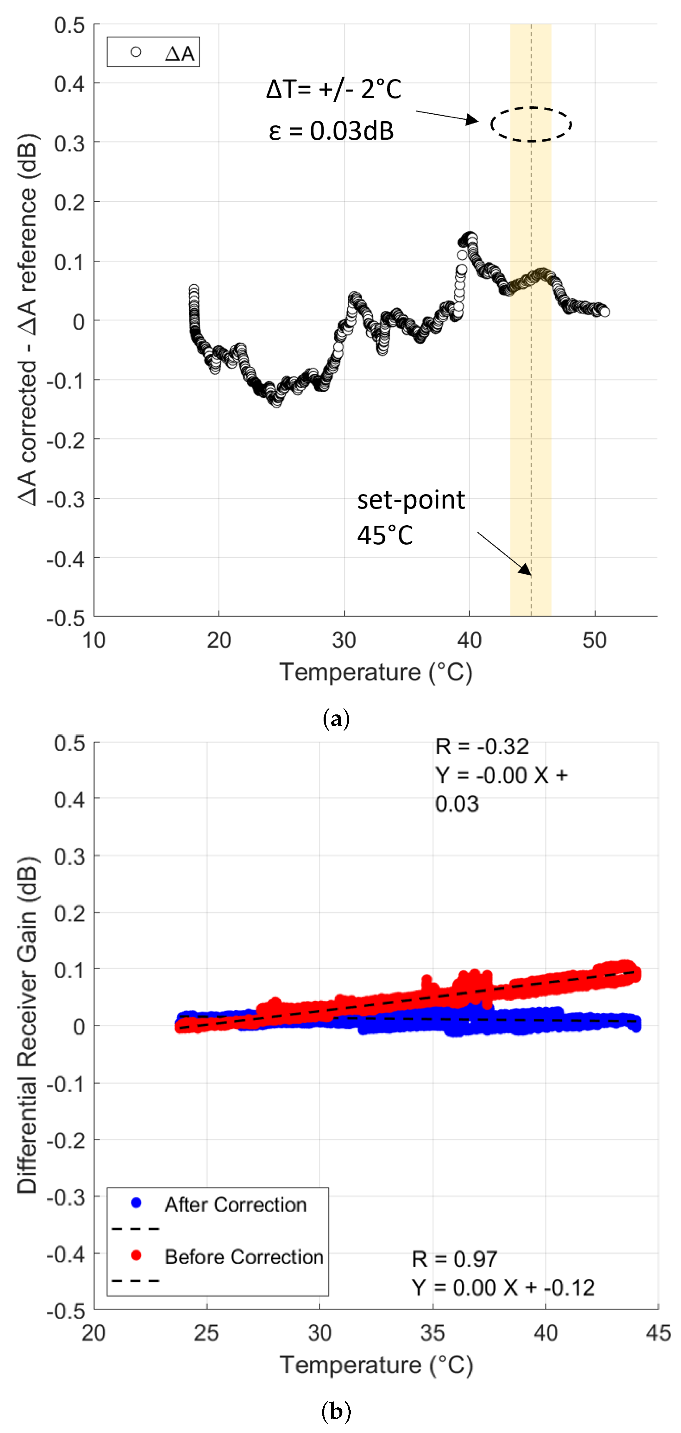
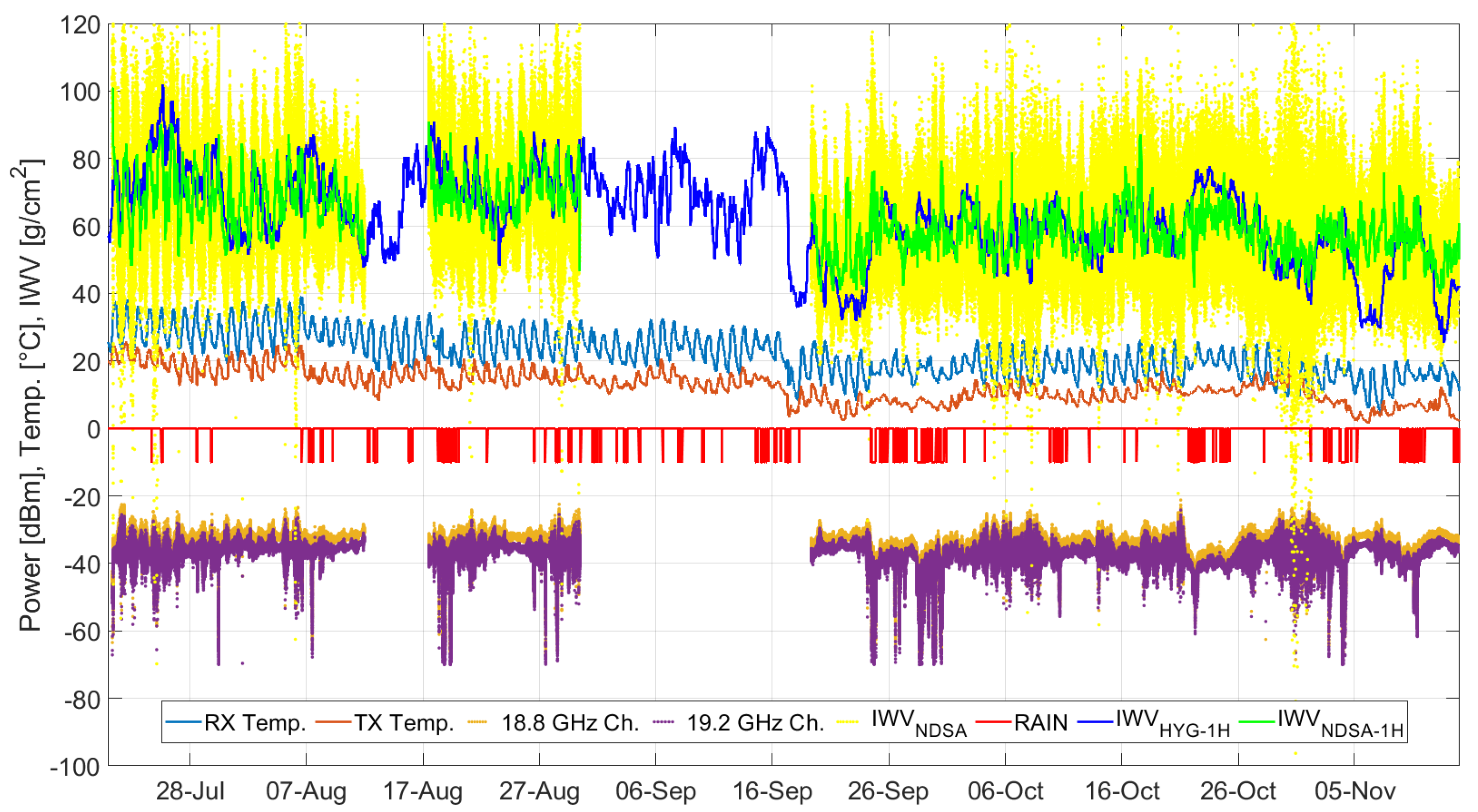
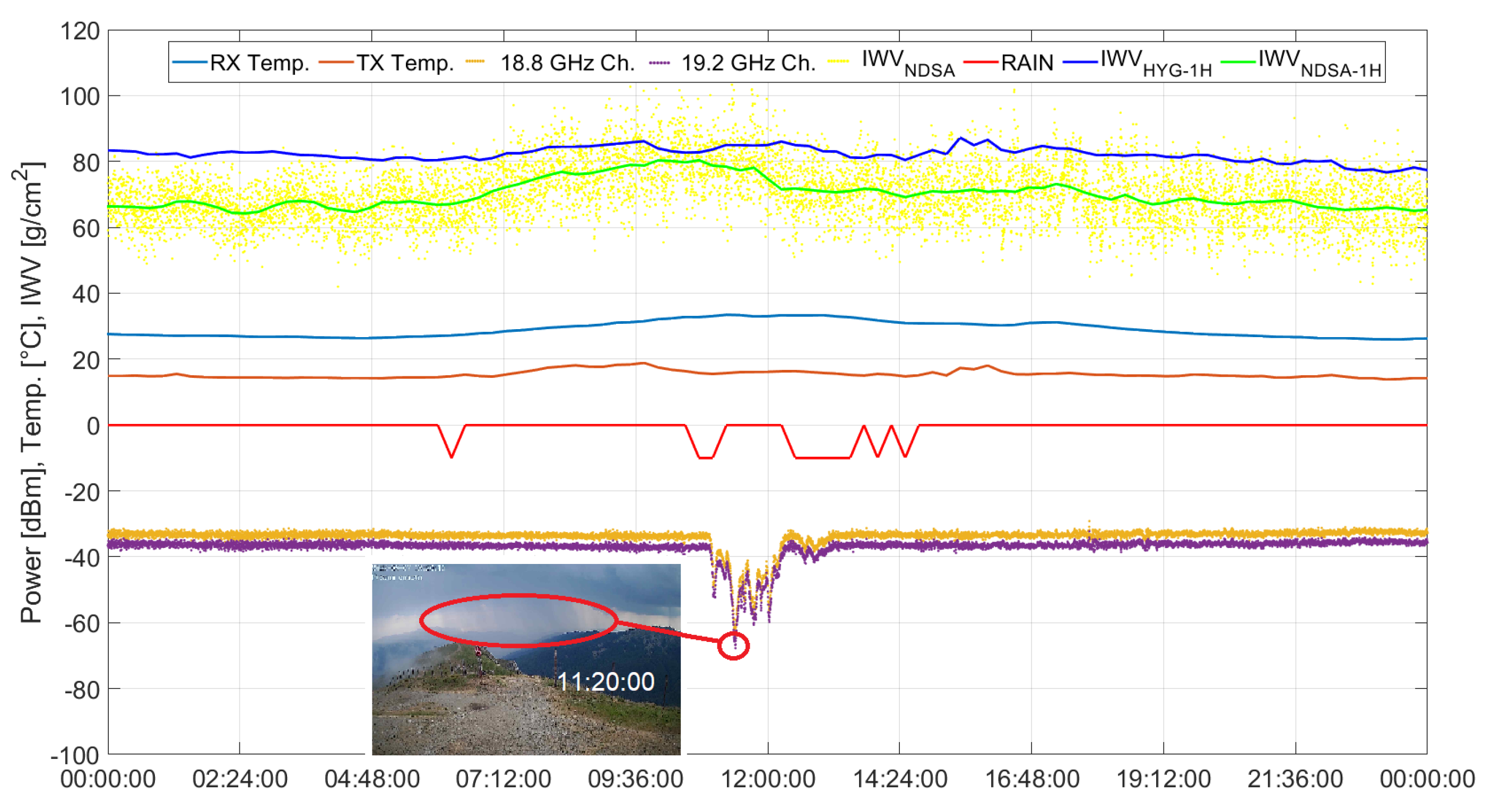
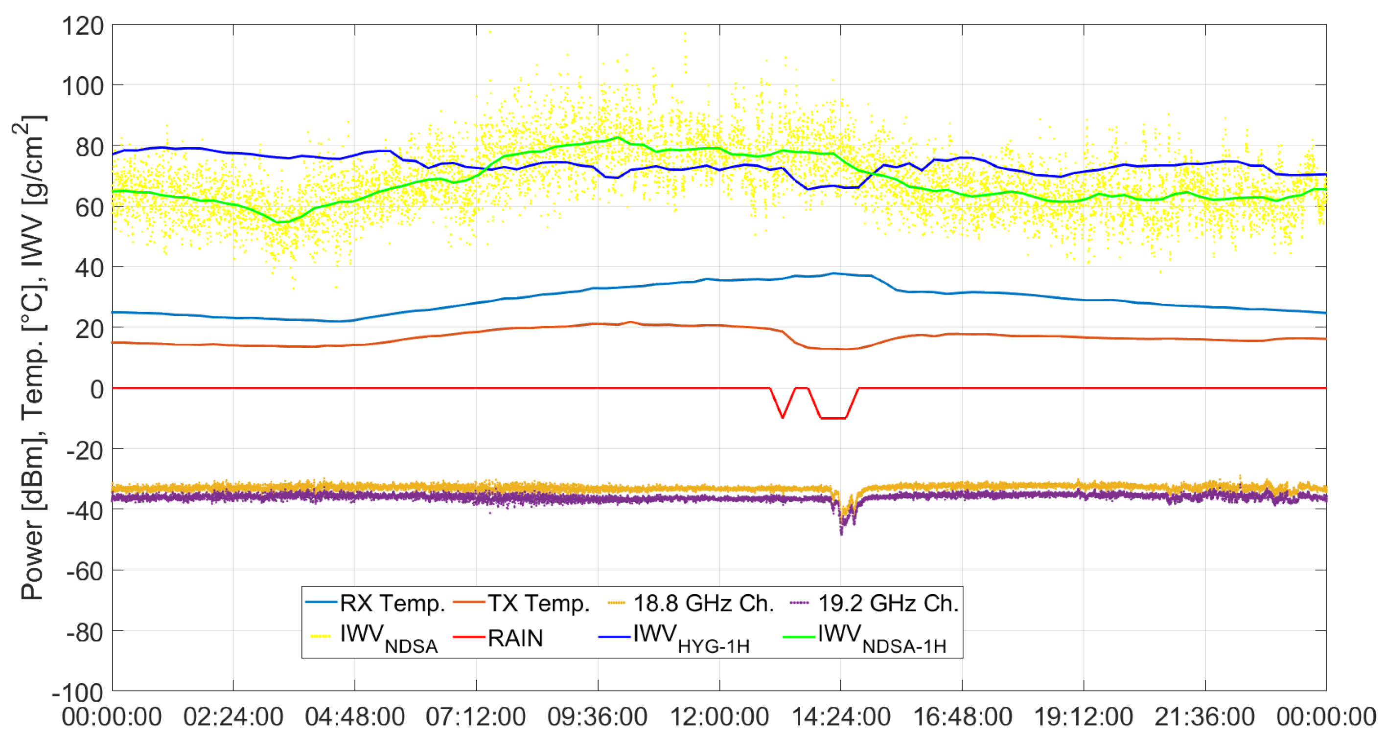
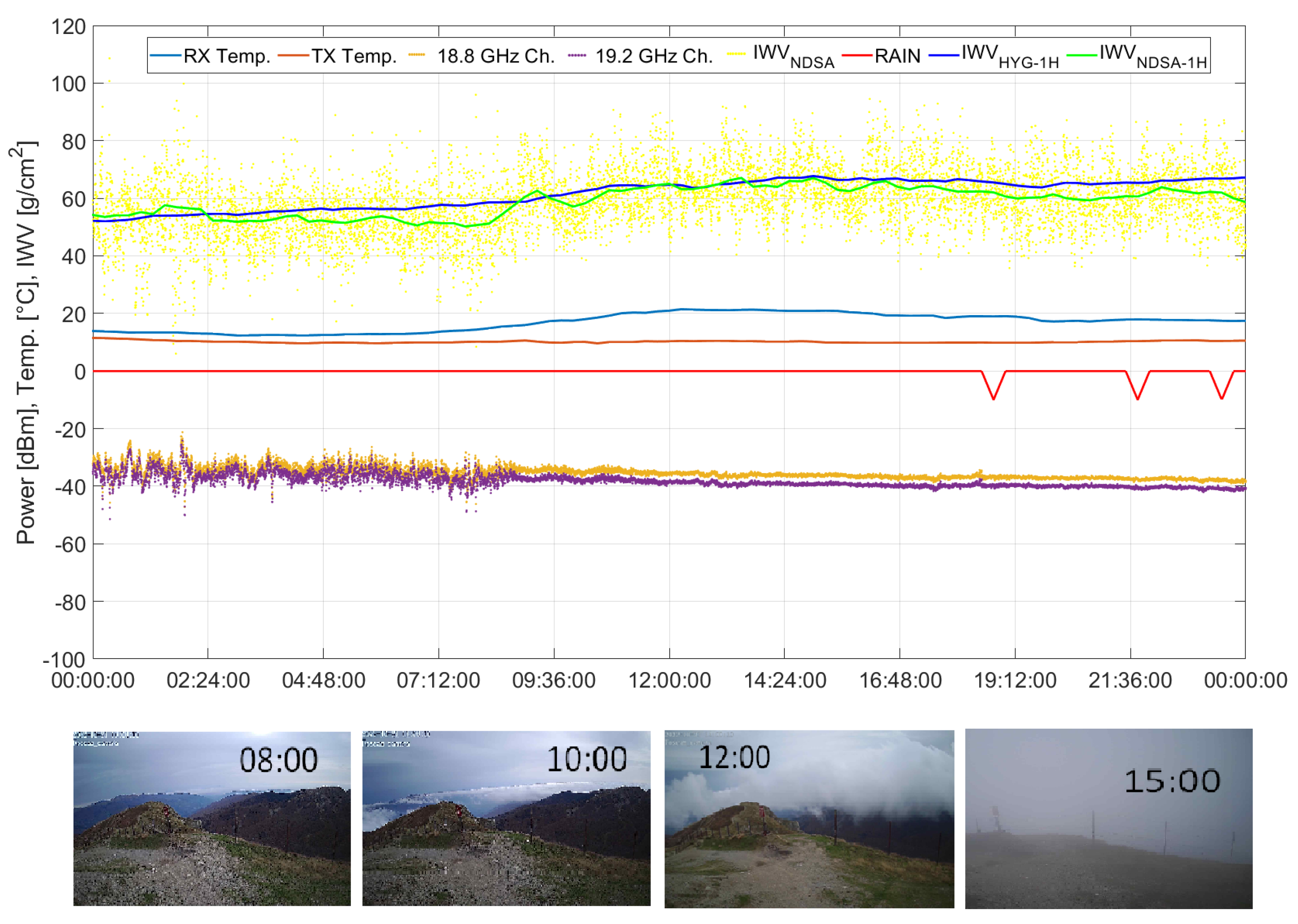
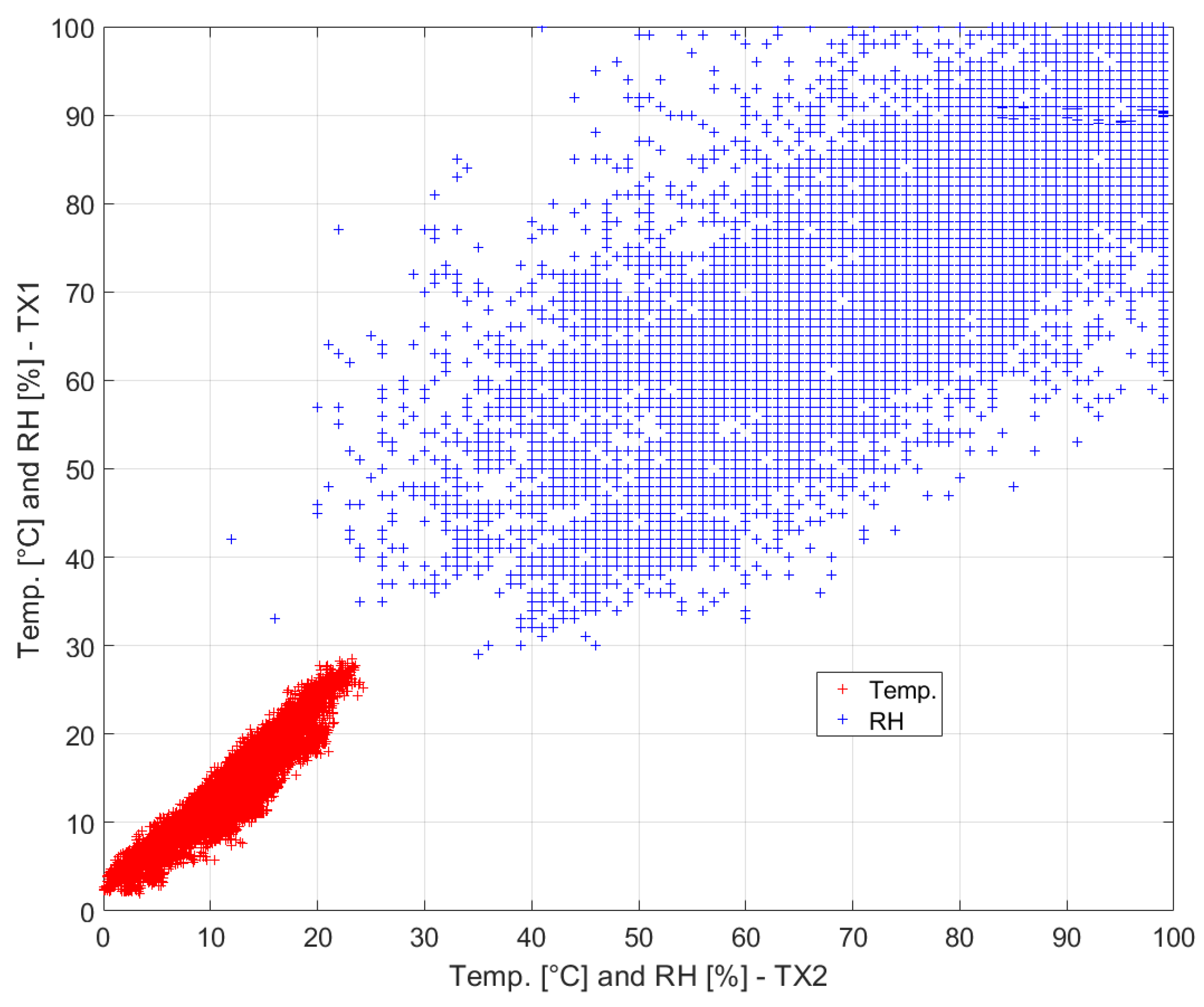
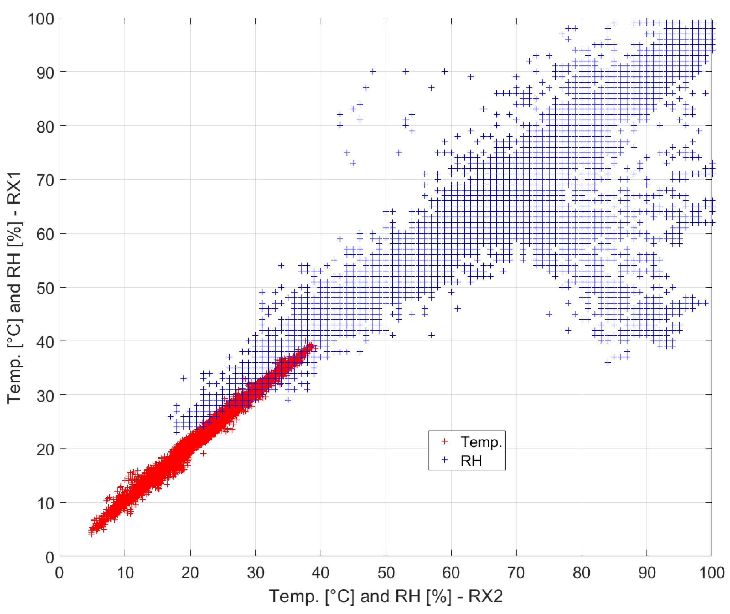
3. Results
4. Discussion
5. Conclusions
Author Contributions
Funding
Data Availability Statement
Conflicts of Interest
Abbreviations
| ADC | Analog to Digital Converter |
| ESA | European Space Agency |
| FIR | Finite Impulse Response |
| FFT | Fast Fourier Transform |
| FPGA | Field-Programmable Gate Array |
| LNB | Low Noise Block |
| IF | Intermediate Frequency |
| LEO | Low Earth Orbiting |
| MPM | Millimeter Wave Propagation Model |
| NDSA | Normalized Differential Spectral Attenuation |
| NWP | Numerical Weather Prediction |
| OCXO | Oven-Controlled Crystal Oscillator |
| PC | Personal Computer |
| PLL | Phase-Locked Loop |
| PM | Power Meter |
| RX | Receiver (or receiving) |
| RF | Radio Frequency |
| RMS | Root Mean Square |
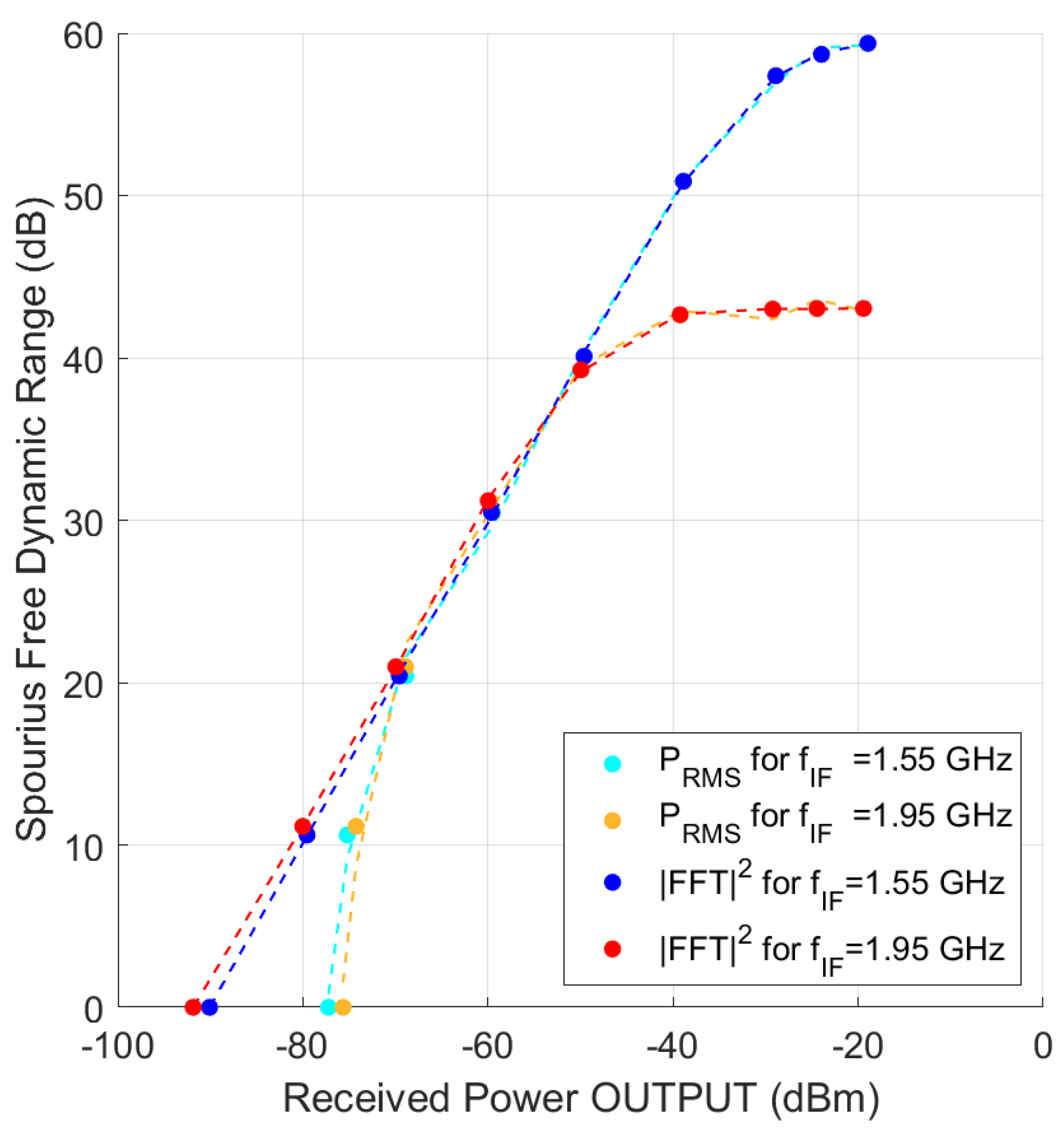
| SFDR | Spurious Free Dynamic Range |
| TX | Transmitter (or transmitting) |
| SDR | Software Defined Radio |
| SWAMM | Sounding Water Vapor by Attenuation Microwave Measurements |
| WV | Water Vapor |
| IWV | Integrated Water Vapor |
References
- Cuccoli, F.; Facheris, L. Normalized differential spectral attenuation (NDSA): A novel approach to estimate atmospheric water vapor along a LEO-LEO satellite link in the Ku/K bands. IEEE Trans. Geosci. Remote Sens. 2006, 44, 1493–1503. [Google Scholar] [CrossRef]
- Facheris, L.; Cuccoli, F.; Argenti, F. Normalized differential spectral attenuation (NDSA) measurements between two LEO satellites: Performance and analysis in the Ku/K bands. IEEE Trans. Geosci. Remote Sens. 2008, 46, 2345–2356. [Google Scholar] [CrossRef]
- Liebe, H.; Hufford, G.; Cotton, M. Propagation Modeling of Moist Air And Suspended Water/Ice Particles at Frequencies below 1000 GHz. In AGARD 52nd Specialists Meeting of the Electromagnetic Wave Propagation Panel on “Atmospheric Propagation Effects through Natural and Man-Made Obscurants for Visible to MM-Wave Radiation”; North Atlantic Treaty Organization: Palma de Mallorca, Spain, 1993. [Google Scholar]
- Facheris, L.; Cuccoli, F. Global ECMWF analysis data for estimating the water vapor content between two LEO satellites through NDSA measurements. IEEE Trans. Geosci. Remote Sens. 2018, 56, 1546–1554. [Google Scholar] [CrossRef]
- Kaufmann, Y.; Gao, B. Remote sensing of water vapor in the near IR from EOS/MODIS. IEEE Trans. Geosci. Remote Sens. 1992, 30, 871–884. [Google Scholar] [CrossRef]
- Li, X.; Dick, G.; Lu, C.; Ge, M.; Nilsson, T.; Ning, T.; Wickert, J.; Schuh, H. Multi-GNSS meteorology: Real-time retrieving of atmospheric water Vapor from BeiDou, Galileo, GLONASS, and GPS observations. IEEE Trans. Geosci. Remote Sens. 2015, 53, 6385–6393. [Google Scholar] [CrossRef]
- Negusini, M.; Petkov, B.H.; Sarti, P.; Tomasi, C. Ground-based water vapor retrieval in Antarctica: An assessment. IEEE Trans. Geosci. Remote Sens. 2016, 54, 2935–2948. [Google Scholar] [CrossRef]
- Tang, A.; Kim, Y.; Xu, Y.; Virbila, G.; Reck, T.; Chang, M.C.F. Evaluation of 28 nm CMOS receivers at 183 GHz for space-borne atmospheric remote sensing. IEEE Microw. Wirel. Components Lett. 2017, 27, 100–102. [Google Scholar] [CrossRef]
- Weaver, D.; Strong, K.; Schneider, M.; Rowe, P.; Sioris, C.; Walker, K.A.; Mariani, Z.; Uttal, T.; McElroy, C.T.; Vömel, H.; et al. Intercomparison of atmospheric water vapour measurements at a Canadian High Arctic site. Atmos. Meas. Tech. 2017, 10, 2851–2880. [Google Scholar] [CrossRef]
- Borger, C.; Schneider, M.; Ertl, B.; Hase, F.; García, O.E.; Sommer, M.; Höpfner, M.; Tjemkes, S.A.; Calbet, X. Evaluation of MUSICA MetOp/IASI tropospheric water vapour profiles by theoretical error assessments and comparisons to GRUAN Vaisala RS92 measurements. Atmos. Meas. Tech. Discuss. 2017, 11, 4981–5006. [Google Scholar] [CrossRef]
- Stevens, B.; Bony, S. What Are Climate Models Missing? Science 2013, 340, 1053–1054. [Google Scholar] [CrossRef]
- Facheris, L.; Cuccoli, F.; Argenti, F.; Martini, E.; Freni, A.; Mori, A.; Mucchi, L. Alternative Measurement Techniques for LEO-LEO Radio Occultation; Final Report ESA-ESTEC Study Contract No. 17831/03/NL/FF; Available at ESA-ESTEC Premises; ESA-ESTEC: Noordwijk, The Netherlands, 2004. [Google Scholar]
- Kirchengast, G.; Schweitzer, S.; Ladstaedter, F.; Gorbunov, M.; Horwath, J.; Facheris, L.; Cuccoli, F.; Martini, E.; Larsen, G.B.; Emde, C.; et al. Study of the Performance Envelope of Active Limb Sounding of Planetary Atmospheres; Final Report ESA-ESTEC Study Contract 21507/08/NL/HE; Available at ESA-ESTEC Premises; ESA-ESTEC: Noordwijk, The Netherlands, 2010. [Google Scholar]
- Facheris, L.; Cuccoli, F.; Martini, E.; Freni, A.; Mazzinghi, A.; Cortesi, U.; del Bianco, S.; Liberti, G.L.; Argenti, F.; Lapini, A.; et al. Analysis of Normalised Differential Spectral Attenuation (NDSA) Technique for Inter-Satellite Atmospheric Profiling; Final Report of the ESA–ESTEC Study Contract No. 4000104831; Available at ESA-ESTEC Premises; ESA-ESTEC: Noordwijk, The Netherlands, 2013. [Google Scholar]
- Facheris, L.; Cuccoli, F.; Martini, E. Tropospheric IWV profiles estimation through multifrequency signal attenuation measurements between two counter-rotating LEO satellites: Performance analysis. In Proceedings of the SPIE 8890, Remote Sensing of Clouds and the Atmosphere XVIII, and Optics in Atmospheric Propagation and Adaptive Systems XVI, Dresden, Germany, 23–26 September 2013; p. 889003. [Google Scholar] [CrossRef]
- Lapini, A.; Cuccoli, F.; Argenti, F.; Facheris, L. The Normalized Differential Spectral Sensitivity Approach Applied to the Retrieval of Tropospheric Water Vapor Fields Using a Constellation of Corotating LEO Satellites. IEEE Trans. Geosci. Remote Sens. 2016, 54, 135–152. [Google Scholar] [CrossRef]
- Mazzinghi, A.; Cuccoli, F.; Argenti, F.; Feta, A.; Facheris, L. Tomographic Inversion Methods for Retrieving the Tropospheric Water Vapor Content Based on the NDSA Measurement Approach. Remote Sens. 2022, 14, 414. [Google Scholar] [CrossRef]
- Di Natale, G.; Del Bianco, S.; Cortesi, U.; Gai, M.; Macelloni, G.; Montomoli, F.; Rovai, L.; Melani, S.; Ortolani, A.; Antonini, A.; et al. Implementation and Validation of a Retrieval Algorithm for Profiling of Water Vapor From Differential Attenuation Measurements at Microwaves. IEEE Trans. Geosci. Remote Sens. 2019, 57, 5939–5948. [Google Scholar] [CrossRef]
- Montomoli, F.; Macelloni, G.; Facheris, L.; Cuccoli, F.; Del Bianco, S.; Gai, M.; Cortesi, U.; Di Natale, G.; Toccafondi, A.; Puggelli, F.; et al. Integrated Water Vapor Estimation Through Microwave Propagation Measurements: First Experiment on a Ground-to-Ground Radio Link. IEEE Trans. Geosci. Remote Sens. 2022, 60, 4101613. [Google Scholar] [CrossRef]
- Cuccoli, F.; Facheris, L.; Cortesi, U.; Del Bianco, S.; Gai, M.; Macelloni, G.; Barbara, F.; Baldi, M.; Montomoli, F.; Antonini, A.; et al. Integrated Water Vapor Estimation Through Microwave Propagation Measurements: Second Experiment on A Ground-to-Ground Radio Link. In Proceedings of the IGARSS 2023—2023 IEEE International Geoscience and Remote Sensing Symposium, Pasadena, CA, USA, 16–21 July 2023; pp. 3788–3791. [Google Scholar] [CrossRef]
- Olsen, R.; Rogers, D.; Hodge, D. The aRbrelation in the calculation of rain attenuation. IEEE Trans. Antennas Propag. 1978, 26, 318–329. [Google Scholar] [CrossRef]
- Doviak, R.J.; Zrnic, D. Doppler Radar and Weather Observations; Academic Press: Cambridge, MA, USA, 1993. [Google Scholar]
- Christofilakis, V.; Tatsis, G.; Chronopoulos, S.K.; Sakkas, A.; Skrivanos, A.G.; Peppas, K.P.; Nistazakis, H.E.; Baldoumas, G.; Kostarakis, P. Earth-to-Earth Microwave Rain Attenuation Measurements: A Survey On the Recent Literature. Symmetry 2020, 12, 1440. [Google Scholar] [CrossRef]
- Martini, E.; Freni, A.; Cuccoli, F.; Facheris, L. Derivation of clear-air turbulence parameters from high-resolution radiosonde data. J. Atmos. Ocean. Technol. 2017, 34, 277–293. [Google Scholar] [CrossRef]
- Martini, E.; Freni, A.; Facheris, L.; Cuccoli, F. Impact of tropospheric scintillation in the Ku/K bands on the communications between two LEO satellites in a radio occultation geometry. IEEE Trans. Geosci. Remote Sens. 2006, 44, 2063–2071. [Google Scholar] [CrossRef]


| Type | |
|---|---|
| vs. T | 0.03 |
| vs. T | 0.04 |
| RX gain linearity (full range) | 0.12 |
| RX gain linearity (Hi SNR) | 0.05 |
| Total (full range) | 0.19 |
| Total (Hi SNR) | 0.12 |
| Station ID | Latitude [°] | Longitude [°] | Altitude a.s.l. [m] |
|---|---|---|---|
| RX1 | 43.8193028 | 11.1680350 | 33 |
| RX2 | 43.7987883 | 11.2511400 | 84 |
| TX1 | 44.1390944 | 10.6735397 | 1345 |
| TX2 | 44.1182556 | 10.6092639 | 1674 |
Disclaimer/Publisher’s Note: The statements, opinions and data contained in all publications are solely those of the individual author(s) and contributor(s) and not of MDPI and/or the editor(s). MDPI and/or the editor(s) disclaim responsibility for any injury to people or property resulting from any ideas, methods, instructions or products referred to in the content. |
© 2024 by the authors. Licensee MDPI, Basel, Switzerland. This article is an open access article distributed under the terms and conditions of the Creative Commons Attribution (CC BY) license (https://creativecommons.org/licenses/by/4.0/).
Share and Cite
Facheris, L.; Cuccoli, F.; Cortesi, U.; del Bianco, S.; Gai, M.; Macelloni, G.; Montomoli, F. A New NDSA (Normalized Differential Spectral Attenuation) Measurement Campaign for Estimating Water Vapor along a Radio Link. Remote Sens. 2024, 16, 3735. https://doi.org/10.3390/rs16193735
Facheris L, Cuccoli F, Cortesi U, del Bianco S, Gai M, Macelloni G, Montomoli F. A New NDSA (Normalized Differential Spectral Attenuation) Measurement Campaign for Estimating Water Vapor along a Radio Link. Remote Sensing. 2024; 16(19):3735. https://doi.org/10.3390/rs16193735
Chicago/Turabian StyleFacheris, Luca, Fabrizio Cuccoli, Ugo Cortesi, Samuele del Bianco, Marco Gai, Giovanni Macelloni, and Francesco Montomoli. 2024. "A New NDSA (Normalized Differential Spectral Attenuation) Measurement Campaign for Estimating Water Vapor along a Radio Link" Remote Sensing 16, no. 19: 3735. https://doi.org/10.3390/rs16193735