A Study of the Mixed Layer Warming Induced by the Barrier Layer in the Northern Bay of Bengal in 2013

Abstract

Strong salinity stratification induced by large freshwater fluxes in the northern Bay of Bengal (BOB) results in the formation of a quasi-permanent barrier layer (BL) that covers almost the entire BOB and leads to a unique temperature inversion within the thick BL in winter. In the presence of temperature inversions, the entrainment process at the bottom of the mixed layer (ML) induces warming effects in the ML, but little is known about this. In this paper, we quantify the contribution of the entrainment process to the ML temperature (MLT) in the northern BOB during the winter of 2013 using monthly and daily data from the Ocean General Circulation Model for the Earth Simulator version 2 (OFES2). It is found that the warming effect of the daily entrainment heat flux (EHF), which resolved the high-frequency variations, is 4 orders of magnitude larger than the monthly EHF for most of the wintertime. This significantly enhanced warming effect in daily data offsets up to 87% of the surface cooling induced by net heat flux during wintertime. A further analysis reveals that the larger daily EHF warming effect compared to its monthly counterpart is closely related to the deepened ML, the larger temperature difference within the ML and vertical velocity at the bottom of the ML.

1. Introduction

In the upper ocean, the formation of a layer with uniform temperature and density, known as the oceanic mixed layer (ML), is influenced by factors such as wind mixing or thermal convection. In most parts of the global ocean, the depth of the ML (MLD) is dominated by the stratification of temperature. Consequently, the MLD usually corresponds to the isothermal layer (IL; Figure 1). However, in the tropical oceans and major estuaries, the strong near-surface salinity stratification, induced by a large amount of freshwater input from precipitation and river discharge, can lead to a shallower ML above the base of the IL. The layer between the base of the IL and the base of the ML is known as the barrier layer (BL) [1]. The BL impedes heat exchange between the ML and the deep ocean and plays an important role in modulating the surface heat budget, sea surface temperature (SST), and thus the coupled air–sea interactions [2,3,4]. With the presence of the BL, the solar shortwave radiation can penetrate through the ML and accumulate within the BL, leading to an increase in the temperature within the BL [5]. Moreover, as the sea surface cools in winter, the ML temperature (MLT) decreases significantly, which results in warmer water in the BL than at the surface, which is known as temperature inversion (Figure 1) [6]. Then, the entrainment process may bring warmer water from the BL into the ML and lead to a warming effect on the ML [7]. This warming effect can have a significant impact on the regional climate. For example, it can exert a vital influence on the intensity of tropical cyclones [8] and the onset of the South Asian monsoon [9].

The Bay of Bengal (BOB), a tropical semi-enclosed basin strongly influenced by the Indian monsoons, is characterized by large freshwater influx from rivers as well as excess monsoonal precipitation over evaporation [10]. The abundant freshwater flux makes the upper layers in the BOB the freshest in the Indian Ocean, and has a substantial influence on the vertical stratification of the upper ocean [11,12,13]. Consequently, quasi-permanent BLs are found in the BOB throughout the year [14,15], and have remarkable seasonal variabilities with notably pronounced BLs in the northern bay during summer and winter [16]. Many studies have been conducted to understand the dynamics of such seasonal variabilities of BLs in the bay. The redistribution of low-salinity waters induced by the surface seasonal circulation has a dominant influence on the extent and BL thickness (BLT) during summer and winter [17]. Other processes such as Ekman pumping and propagating Rossby waves forced by Kelvin waves along the eastern boundary also modulate the variations in the BLs [18,19].

Corresponding with the spatiotemporal variations in the BLs mentioned above, temperature inversion is confined to the northern BOB, specifically to north of 15°N, where the BL is relatively thick during the winter months with sea surface cooling (i.e., November to the following February) [20]. Correspondingly, the entrainment process occurring within the warm BL that leads to ML warming is predominantly observed during the winter months, as expected, and contributes to the seasonal and interannual variability of the SST in the northern bay [21,22,23,24,25,26,27]. However, based on the monthly observational data or model output, the results show that the contribution of the entrainment heat flux (EHF) to ML warming is rather small, at approximately one order of magnitude smaller than that of atmosphere heating [24,26,27]. In contrast, the Southern Ocean is also characterized by the warm BL underlying the cool ML in austral winter, and thus provides a unique heating effect on the ML through the entrainment processes at the base of the ML, similar to the BOB [28]; however, in the Southern Ocean, the comparison between the daily and monthly EHF warming indicates that the high-frequency variations in the ML resolved in the daily data can contribute to mixed layer warming nearly twice as much as the monthly data in the BL period, which is enough to compensate for or even surpass the surface heat loss. They argue that this larger degree of warming in the daily results is due to the stronger relative rate of the MLD deepening and larger temperature differences between the ML and the layer immediately below. Similar results were reported by Foltz et al. (2009) [29]. They found that in the central Tropical North Atlantic, a daily time series observed by a buoy at 15°N 38°W clearly detected a 1–2-month intermittent warming of the ML induced by the EHF under temperature inversion conditions during December–February, while the warming disappeared when the EHF is averaged to the monthly climatological means.

Compared to the results in the Southern Ocean and the North Atlantic [28,29], the relatively small contribution from the EHF to the MLT with large residuals has been shown in the aforementioned studies [24,26,27] in the BOB. Due to a lack of observations, these studies on the seasonal and interannual variations in the heat budget of the ML in the BOB merely relied on monthly data, and resulted in a relatively small EHF and large residuals. By using monthly data, high-frequency variations and their contributions to mixing and entrainment are not included in the EHF [28] and consequently result in large residuals. Till now, the contribution of the EHF to the variations in the MLT in the BOB by considering high-frequency processes has not been properly assessed. Such studies could expand our understanding of the role of salinity and the BL on the regional climate and related dynamic mechanisms, which may contribute to the prediction of South Asian monsoons and tropical cyclones with a reasonable consideration of the influence of salinity and the BL in the model.

Therefore, in this study, we employ a comparative analysis using daily and monthly model outputs to investigate the differences in the EHF calculated from these two temporal resolutions during the winter temperature inversion period and discuss the related mechanisms. The rest of this paper is organized as follows: Section 2 introduces the data and methods, Section 3 analyzes the impacts of winter BLs on the MLT by comparing the daily and monthly results, and Section 4 presents the conclusion and discussion.

2. Data and Methods

2.1. Data

The temperature, salinity, current, and surface net heat flux data employed in this study are from the Ocean General Circulation Model for the Earth Simulator version 2 (OFES2) provided by the Japan Agency for Marine-Earth Science and Technology (JAMSTEC) [30]. The OFES2 is based on the Modular Ocean Model version 3 (MOM 3) and utilizes a latitude and longitude grid system. Previous studies have suggested that this dataset has successfully simulated the upper layer thermohaline structure and ocean circulation in the BOB [25,31,32]. It provides both monthly and daily resolved data, and thus facilitates an evaluation of the contribution of the entrainment processes associated with high-frequency processes. Both the daily and monthly datasets cover the period from January 1958 to December 2022, with a spatial resolution of 0.1° × 0.1° and 105 vertical layers. There are 44 layers above 300 m. The wind data driving the OFES2 model is from the Japanese 55-year atmospheric reanalysis-based surface dataset for driving ocean–sea ice models (JRA55-do) [33], and it is used to explore the relationship of the high-frequency variations between surface wind and the EHF.

In the BOB, the Indian Ocean Dipole (IOD) and El Niño–Southern Oscillation (ENSO) can greatly induce interannual variability in the BLT [18,34]. To isolate such interannual signals in the BLT associated with the IOD and ENSO, we selected a normal year of 2013 during the Argo period (i.e., after 2003), and compare the effects of the EHF on the MLT between monthly and daily data under the normal conditions of the BLT during that year. Thus, the OFES2 dataset from September 2013 to April 2014 is used in this study. OFES2 temperature and salinity data are used to calculate the MLD, IL depth (ILD) and BLT. In addition, these two types of data, together with surface heat flux and ocean current data, are used in the analysis for the ML heat budget.

Monthly Argo temperature and salinity data from the Asia-Pacific Data-Research Center (http://apdrc.soest.hawaii.edu, format: accessed on 8 March 2024.), covering the same period as the OFES2 dataset (September 2013 to April 2014), with a horizontal resolution of 1° × 1°, are used to validate the BLT results of the OFES2 dataset.

2.2. Methods

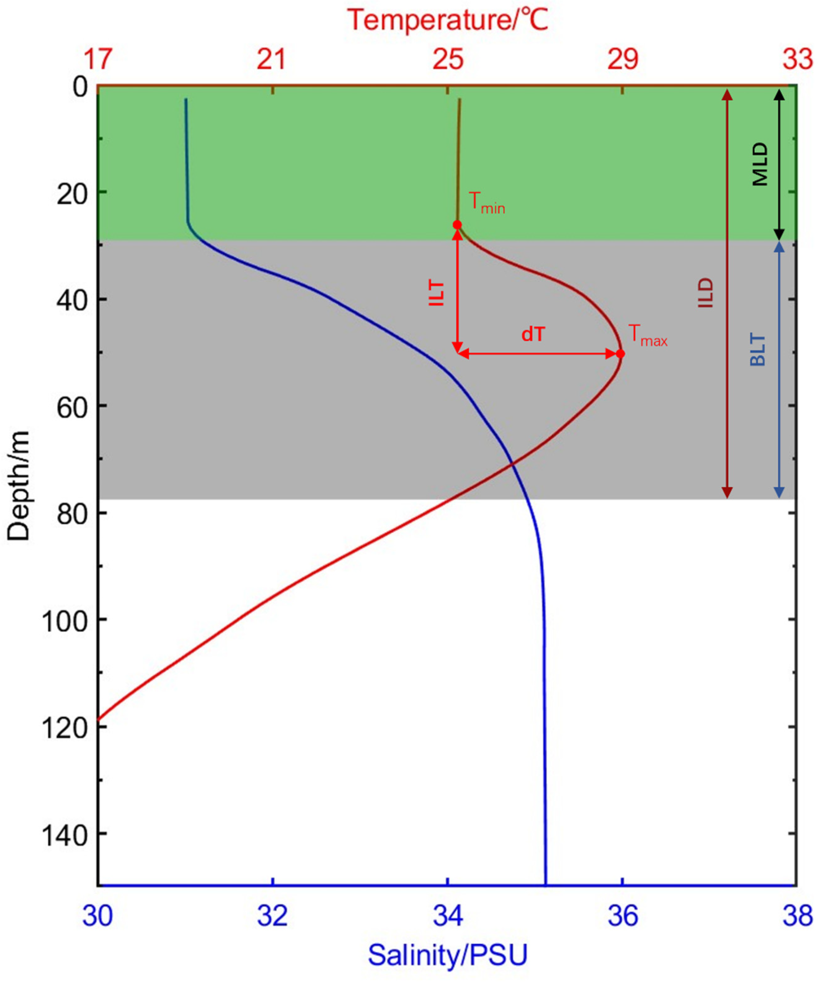
2.2.1. Calculation of ILD, MLD and BLT

The calculation of ILD, MLD, and BLT follow the definitions proposed by De Boyer Montégut et al. [15]. ILD is defined as the depth where temperature decreases by 0.2 °C relative to the 10 m layer. Similarly, the MLD is defined as the depth where potential density ${\sigma }_{\theta }={\sigma }_s+{\sigma }_{\Delta }$, with ${\sigma }_s$ being the potential density at 10 m, and ${\sigma }_{\Delta }$ representing the increase in potential density due to a constant salinity relative to the 10 m layer and a temperature decrease of 0.2 °C. BLT is defined as the difference between IL depth and MLD when IL is deeper than ML.

2.2.2. Calculation of Temperature Inversion

The calculation of temperature inversion follows the definition proposed by Li et al. [20]. The temperature inversion layer thickness (ILT) is defined as the depth below 10 m where the temperature increases with depth, and its amplitude (dT) is characterized by the difference between the maximum (T_max) and the minimum (T_min) within the ILT (Figure 1).

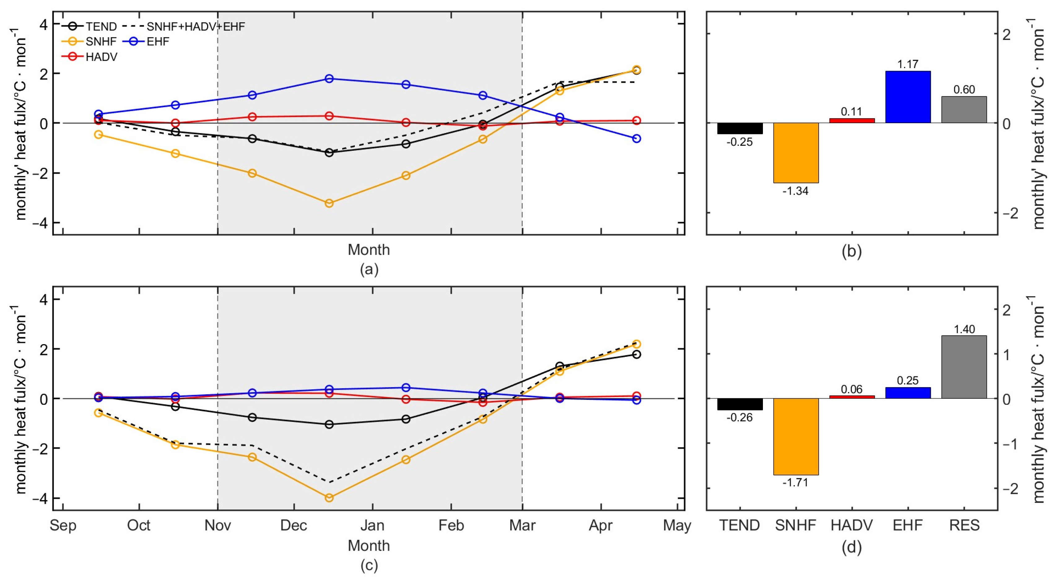
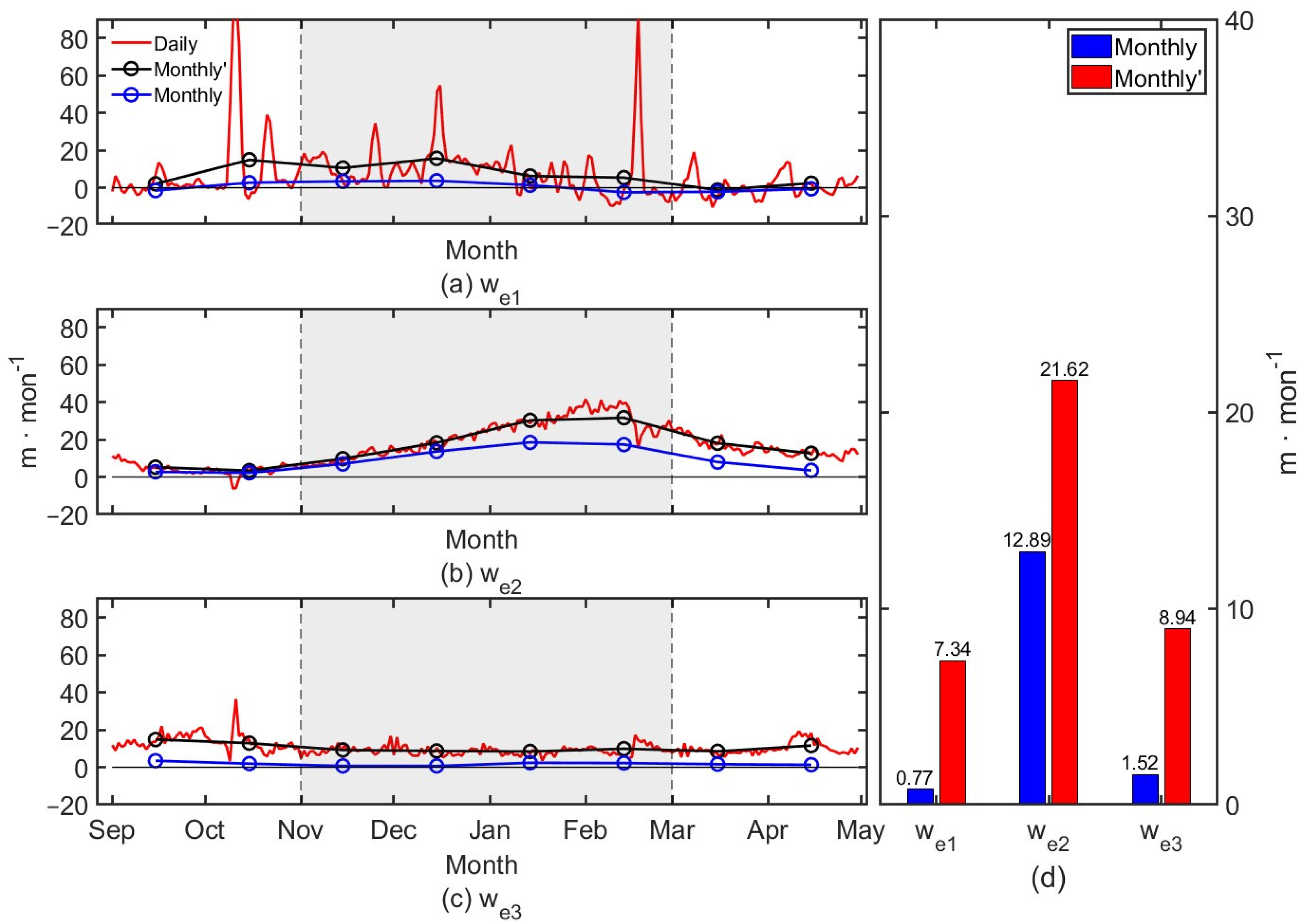
2.2.3. ML Heat Budget

The ML heat budget formula used in this study is based on that from Wang et al. [28]:

$${\displaystyle \frac{\partial T_{ml}}{\partial t}}={\displaystyle \frac{Q_{ml}}{\rho C_{p}h}}-\left(u_{ml}{\displaystyle \frac{\partial T_{ml}}{\partial x}}+v_{ml}{\displaystyle \frac{\partial T_{ml}}{\partial y}}\right)-{\displaystyle \frac{\Delta T}{h}}{w}_e+RES$$

(1)

From left to right, the terms represent the temperature tend (TEND), surface net heat flux (SNHF), horizontal advection heat flux (HADV), entrainment heat flux (EHF) and residual (RES). Here, h is the MLD, $T_{ml}$ is the MLT, $\rho$ is seawater density, $C_p$ is the specific heat capacity, $u_{ml}$ and $v_{ml}$ are the zonal and meridional components of the mean flow in the ML, $Q_{ml}=Q_{net}-Q_{pen}$ is the net heat flux for air–sea exchange within the ML, $Q_{net}$ is the net heat flux at the sea surface, $Q_{pen}=0.47\times Q_{SW}{·e}^{-0.04·\mathrm{h}}$ accounts for shortwave flux penetration through the ML [23], where $Q_{SW}$ is the shortwave radiation, $\Delta T$ is the difference between the average MLT and the temperature below the ML bottom. The formula for entrainment velocity $w_e$ is based on that from Wang et al. [28]:

$$w_e={\displaystyle \frac{\partial h}{\partial t}}+\left(u_{-h}{\displaystyle \frac{\partial h}{\partial x}}+v_{-h}{\displaystyle \frac{\partial h}{\partial y}}\right)+w_{-h}$$

(2)

Here, $-h$ represents the bottom of the ML. The entrainment velocity $w_e$ is decomposed into three terms from left to right: local variations in the ML ($w_{e1}$), lateral induction ($w_{e2}$), and vertical velocity at the bottom of the ML ($w_{e3}$). This study only considers the entrainment processes. When $w_e>0$, entrainment processes are considered while it is set to be zero otherwise ($w_e\le 0$).

Therefore, the EHF consists of the three terms. The local term (Ent1), $-{\displaystyle \frac{\Delta T}{h}}{\displaystyle \frac{\partial h}{\partial t}}$, represents the effect of local MLD variability. The advection term (Ent2), $-{\displaystyle \frac{\Delta T}{h}}\left(u_{-h}{\displaystyle \frac{\partial h}{\partial x}}+v_{-h}{\displaystyle \frac{\partial h}{\partial y}}\right)$, represents horizontal advection across the bottom of the ML. The vertical velocity (Ent3), $-{\displaystyle \frac{\Delta T}{h}}{w}_{-h}$, represents vertical advection across the bottom of the ML.

The $\Delta T$ is the temperature difference between the ML average and the ML base which is hard to determine with the real data. Therefore, the common practice is to use the temperature difference between a fixed depth difference beneath the ML base. Various thresholds of depth beneath the ML base were selected in previous studies, such as 5 m [22,35], 10 m [36,37] and 20 m [38,39]. In the present study, we select 5 m below the ML base and ΔT is calculated as the difference between the average MLT and the temperature 5 m below the ML base. To examine the sensitivity of EHF to the different thresholds of depth, we compare the result of 5 m depth difference (EHF₀₅) with a moderate threshold of 10 m depth difference (EHF₁₀). The difference between the values of EHF₁₀ and EHF₀₅ is small, with its mean value 27.4% higher than that of EHF₀₅ during the winter months (i.e., November–following February) of 2013. This small difference between them underpins the fact that the values of EHF are not very sensitive to the depth if moderate thresholds are selected, such as 5 m or 10 m. Thus, in previous studies, EHF is estimated by using the temperature difference between a fixed depth beneath the mixed layer base, as mentioned above. However, it should be noted that the method we used may overestimate the values of EHF to a certain degree, due to the possible impact of other mixing processes below the mixed layer, such as shear-induced mixing and convective mixing.

3. Results

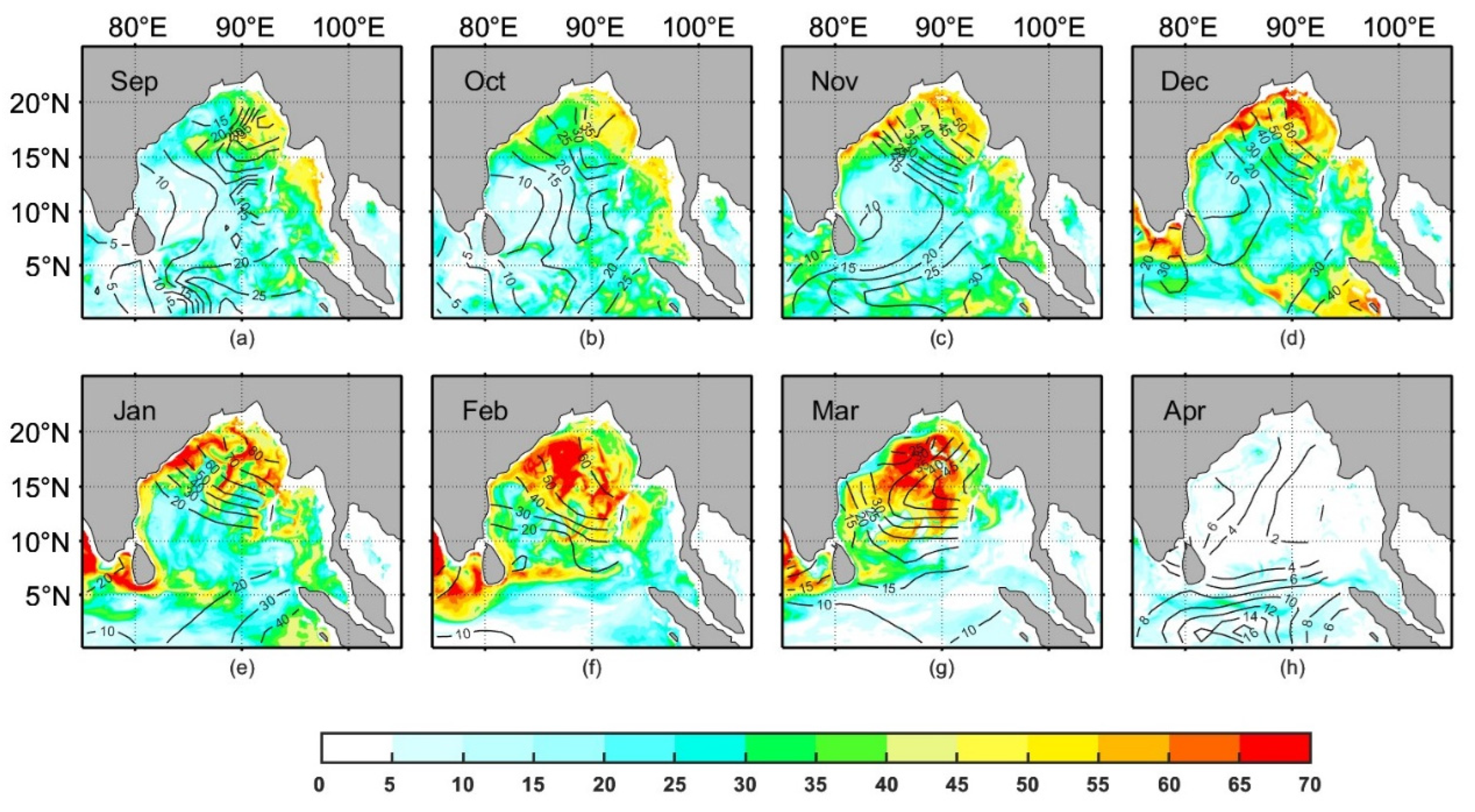
3.1. Distribution of the BL and Temperature Inversion in Winter 2013

Firstly, we conducted a comparative analysis between the BLT calculated from the OFES2 reanalysis data and the results from the Argo observation to validate the reliability of the OFES2 reanalysis dataset (Figure 2). Both of the two datasets show a similar distribution of the BLT. According to the OFES2 data, during autumn (September–October), the BL is relatively thin in most areas of the bay (25 m to 35 m), with thicker layers (45 m to 55 m) observed near the Sunda Strait, the Andaman Sea, and the Myanmar coast. During the winter (November to the following February), the BOB displays a much thicker BL compared to that in the other seasons [18], which persists into early spring (March). Particularly, from December to next March, the BLT in the northern bay (north 15°N) can exceed 60 m, while the southern bay exhibits thinner layers. The thicker BL in the wintertime in the northern bay is partly contributed by the shallower ML associated with the southward transport of the freshwater input from the northern tip of the bay [17]. Additionally, a region near the Sunda Strait also presents thick BLs during December and January. In April, the BLT throughout the bay is generally less than 5 m. In general, these OFES2 results agree well with the Argo observations in terms of the spatial distribution patterns and seasonal variations in the BL, except for those from the Andaman Sea, which is blanked in the Argo results due to the few Argo observations there. In addition, the OFES2 results indicate that the thickest BL is located in the central bay between 14° and 19°N, and the BL in the northern bay (>19°N) is much thinner than that in the central bay (Figure 2f). However, the Argo results show that the BLT decreases southward. Thus, the noticeable difference in the BL distribution between these two types of data is located in the northern bay, and this is due to the sparse Argo data in that region. Despite these differences, the general consistency between the two datasets, although the slightly smoother appearance of Argo data due to its lower spatial resolution, underscores the ability of OFES2 to reliably depict the distribution and variations in the BL in the study region.

Figure 3 displays the monthly distribution of the dT. Temperature inversions mainly occur in the northern BOB (north 15°N) during winter, which is generally consistent with the spatial extent of the thick BL. The temperature inversion begins in November at the northern tip of the bay and gradually extends southward. Both the spatial coverage and the amplitude reach peaks in January, with a maximal dT up to 3.0 °C. From February, the distribution of the temperature inversion recedes northward, accompanied by a corresponding decrease in the amplitude. By April, the temperature inversion completely disappears due to the rise in the SST. This phase-locking of the temperature inversion in the northern bay during the winter months is predominantly attributed to the unique wintertime ocean–atmosphere forcings. Previous studies [22] suggest that this is attributed to the intense latent heat release from the dry and cold winter monsoon winds, leading to a substantial cooling of the ML. In addition, the advection of fresh water input from the rivers around the northern boundary of the bay also plays a role in maintaining the thicker BL and the temperature inversion in it. In the presence of winter temperature inversion, the ocean dynamic processes such as advection and entrainment at the bottom of the ML result in the transfer of warmer water from the BL to the ML and consequently warm the ML from the subsurface [24]. In the following sections, we will analyze the impact of entrainment processes in the BL on the MLT in the winter of 2013, based on the heat budget equation of the ML mentioned in Section 2.2.

3.2. Impact of Winter BLs on the Temperature of the ML: Comparative Analysis between Daily and Monthly Data

The entrainment process is a small-scale vertical transport process that persists over a long time scale. Therefore, the cumulative effects of high-frequency eddy advection variations are expected to differ significantly from monthly averaged data. To clarify the impact of high-frequency processes, we chose Region A (87°E–94°E, 15°N–21°N, as shown in Figure 3e) to calculate the ML heat budget. Region A is characterized by a thick BL and significant dT in the northern bay (Figure 2 and Figure 3e). Figure 4 displays the time series of the EHF in the ML over Region A calculated using daily and monthly OFES2 data. The differences between the daily and monthly EHF are mainly observed from November to the following February. Both the results from the daily and monthly data are positive, but the daily EHF is larger than that from the monthly results most of the time. This difference increases with the temperature inversion, and decreases after reaching a maximum in December. The maximum daily EHF can be up to 3.49 °C/month, which is nearly an order of magnitude higher than the monthly values. The accumulating daily EHF in each month (monthly’ EHF) is 1.12–1.79 °C/month during November to the following February (Figure 4a), with an average value of 1.17 °C/month, which is 4 times larger than the monthly result (Figure 4b). The difference arises because the daily results not only include the low-frequency entrainment processes resolved by the monthly data, but also incorporate the EHF induced by high-frequency variations, which is almost absent in the monthly data.

Merely relying on the monthly data, the previous studies have reported that the SNHF is the dominant factor affecting the heat budget of the ML in the BOB during winter, while the contributions of HADV and EHF are one order smaller than that of SNHF [24,27]. As the monthly data cannot properly detect the high-frequency processes, it may underestimate the role of EHF, and results in the large residual term partly associated with the high-frequency variations [24,27]. Using the same monthly resolution data as in the previous studies, we can see that the monthly EHF tends to warm the ML and offsets the surface cooling induced by the SNHF, but its contribution is very small, as expected (Figure 5b), which is consistent with previous studies [24,27]. The absolute ratio of it to the value of the SNHF is around 10% in most of the winter months. In contrast, when accounting for the impact of high-frequency variations, the EHF obtained from the daily data exhibits a more significant warming effect on the MLT (Figure 4 and Figure 5a). This warming effect greatly weakens the surface cooling associated with the SNHF. The absolute daily ratio of the warming effect of the EHF to the value of the SFHF cooling effect is approximately 50% in November and December, and surpasses 90% in January and February (Figure 5a). Similarly, the absolute ratio of the monthly’ EHF warming effect to the cooling value of the monthly’ SFHF cooling effect exceeds 50% during these winter months, and is much larger than the monthly EHF results (Figure 5b; black line vs. blue line).

Figure 6 compares each heat budget term in the ML between the daily and monthly data. For the monthly data, the surface cooling trend of −0.26 °C/month is dominated by the SNHF (−1.71 °C/month). The warming effect from HADV and EHF is very weak (0.06 °C/month and 0.25 °C/month, respectively), which only offsets 18% of the overcooling caused by the SNHF. Consequently, the RES is very large (Figure 6c; the solid black curves vs. the dash black curves), with the averaged value reaching up to 1.40 °C/month, close to the dominant term of the SNHF (Figure 6d). The large RES may be due to the contributions from the high-frequency EHF and the other mixing processes which are absent in the monthly data. For the daily data, the surface cooling trend of −0.25 °C/month is also primarily caused by the SNHF (−1.34 °C/month), which is consistent with the monthly results. However, the significantly enhanced monthly’ EHF makes the RES rather small (Figure 6a; the solid black curves vs. the dash black curves). It has an averaged value of 1.17 °C/month during wintertime and offsets 87% of the SNHF cooling, resulting in a relatively small RES value (0.60 °C/month; Figure 6b). These differences in the daily and monthly results underpin the fact that the analysis of the heat budget of the ML using daily data can give a more reliable estimation of the heat balance due to the more accurate EHF term in the daily results.

The aforementioned daily EHF is greatly enhanced compared to the monthly EHF in the winter months. Considering that the entrainment term consists of the local term (Ent 1), the advection term (Ent 2), and the vertical velocity term (Ent3), we further analyzed the contributions of these three terms to the winter EHF. Figure 7 shows their contributions during the period from September to April. Large difference in Ent1 between the daily and monthly results primarily appears in the winter months, peaking in December or January (Figure 7a). On average, for the winter months (i.e., November to the following February), the daily Ent1 is 0.30 °C/month, 0.25 °C/month larger than the monthly Ent1 (Figure 7d). Similarly, the daily Ent2 and Ent3 have larger values compared to the monthly results, with a difference of 0.34 °C/month and 0.39 °C/month, respectively. Therefore, the analysis above reveals that these three terms have a comparable contribution to the larger degree of warming of the ML in the daily EHF compared to the monthly results in winter.

As shown in Equations (1) and (2), Ent1, Ent2 and Ent3 are all directly controlled by the T_h term: the ratio of the temperature difference within the ML to the MLD ($-{\displaystyle \frac{\Delta T}{h}}$). In addition, they are also affected by local variations in the ML ($w_{e1}$), lateral induction ($w_{e2}$), and vertical velocity at the bottom of the ML ($w_{e3}$), respectively. As shown in Figure 8a, the difference in the T_h term is large between the daily and monthly results, and it is primarily caused by $\Delta T$ (Figure 8b,c). In general, the averaged value of the daily T_h term is twice as large as that of the monthly T_h term (0.02 °C/m vs. 0.01 °C/m; Figure 8d), which is dominated by the difference between the daily $\Delta T$ and monthly $\Delta T$ (0.63 °C vs. 0.30 °C), partly contributed by the difference from the MLD (17.15 m vs. 14.08 m; Figure 8e,f).

Besides the aforementioned effect from the T_h term, $w_{e1}$, $w_{e2}$ and $w_{e3}$ also contribute to Ent1, Ent2 and Ent3, respectively (Figure 9). We can see that both the daily $w_{e1}$ and $w_{e3}$ are approximately 5 times larger than the monthly results (Figure 9a–c). In contrast, the average value of the daily $w_{e2}$ is 68% larger (21.62 m/month vs. 12.89 m/month) than that of the monthly $w_{e2}$ (Figure 9b,c). Therefore, the enhanced Ent1 and Ent3 are mainly caused by $w_{e1}$ and $w_{e3}$, and $\Delta T$ plays a secondary role. In contrast, the difference between the daily and monthly Ent2 result primarily comes from $\Delta T$, and $w_{e2}$ also makes an important contribution.

4. Discussion

In the BOB, as the daily data include high-frequency processes, the EHF warming calculated from the daily data can give a more reliable estimation of the role of the BL on the MLT. Both the daily EHF and the monthly values averaged from it are much larger than those calculated directly from the monthly data (e.g., Figure 4). Thus, the EHF estimated using the monthly numerical model output of the turbulent heat flux is expected to be more accurate than the results estimated directly from the monthly model outputs.

According to previous studies, the enhanced EHF in the daily data compared to that in the monthly data is probably related to high-frequency fluctuations in surface wind fields [40]. Therefore, we discussed the short-timescale fluctuations in the MLD and $\Delta T$ in relation to winds. Considering that, in JRA55-do, wind is used as the surface forcing of the OFES2 model [6], we therefore construct the daily JRA55-do wind from the original 3 h wind forcing of OFES2 to explore its possible impact on the high-frequency variations in the MLD and ΔT. Figure 10a shows the power spectrum of the MLD, ΔT and surface wind speed during the 2013 winter months (i.e., November to the following February). One can see that there are several significant peaks of energetic oscillation of the surface wind found within the time bands 10–30 and 5–10 days, corresponding to the sub-monthly and weekly oscillations, respectively. Similarly, the MLD time series shows high variabilities at these two time bands, and ΔT indicates strong oscillations in the sub-monthly band. Furthermore, the correlation coefficients of the MLD and ΔT with the surface wind speed are significant at the 95% confident level at these frequencies (Figure 10b). The consistencies between them implies that surface wind is likely the major forcing factor for the high-frequency variations in the MLD and ΔT on the sub-monthly time scales. That is to say, the high-frequency fluctuations in the EHF were likely driven by sea surface wind during winter 2013.

5. Conclusions

In this study, we utilize OFES2 reanalysis together with Argo observations to explore the ML warming induced by the BL over the BOB during the winter of 2013. Firstly, a comparison with the Argo results indicates that OFES2 data accurately captures the spatial distribution and seasonal variation characteristics of the BL and temperature inversion in the winter of 2013, validating the reliability of OFES2 data.

Based on the mixed-layer heat budget formula, we investigated the impacts of the winter entrainment process in the BL to the variations in the MLT. The analysis reveals that the presence of temperature inversion within the BL results in a warming of the ML in both the daily and monthly EHF data. However, the daily EHF values are 4 orders of magnitude higher than the monthly EHF values for most of the winter months. This suggests that the monthly data, due to its inability to resolve the high-frequency process which is present in the daily data, consequently underestimates the contribution of EHF. Therefore, the warming effect of the monthly EHF can inevitably underestimate the contribution of the BL to the temperature of the ML. Consistent with previous studies [24,27], our analysis indicates that the absolute ratio of its contribution to the SNHF is approximately 10% in most of the winter months. In contrast, the ratio of the monthly EHF warming effect calculated from the daily data to the SNHF is larger than 50%. This significantly enhanced EHF (i.e., monthly’ EHF) offsets up to 87% of the SNHF cooling effect during wintertime, resulting in a relatively small RES value. This result underlines that the analysis of the heat budget in the ML using daily data may give a more reliable estimation of the heat balance due to the more accurate EHF term in the daily results.

A further analysis reveals that the significantly enhanced daily EHF in winter is caused by the three vertical terms, including the local term (Ent1), the advection term (Ent2) and vertical velocity term (Ent3), which have a comparable contribution to the warming of the ML in the daily EHF values. Moreover, the strengthened Ent1 and Ent3 were mainly induced by the enhanced local variations in the ML and vertical velocity at the bottom of the ML, respectively, while Ent2 is dominated by $\Delta T$. Hence, we explore the relationship between the high-frequency variations in the surface wind and the MLD and $\Delta T$, both of which contribute to the enhanced daily EHF values. This reveals that the high-frequency variations in the MLD and $\Delta T$ are likely induced by surface wind, and consequently lead to the enhanced daily EHF associated with high-frequency processes.

The high-frequency BL entrainment process plays a vital role in modulating the SST, and its cumulative effects over a long time scale are expected to have important impacts on the seasonal or even interannual variability in the SST in the northern BOB. By considering the EHF induced by the high-frequency processes in the ML, how and to what extent the BL affects the low-frequency variability in the SST and the associated air–sea interaction processes can be studied further.

References

1. Godfrey, J.S.; Lindstrom, E.J. The Heat Budget of the Equatorial Western Pacific Surface Mixed Layer. J. Geophys. Res. 1989, 94, 8007–8017. [Google Scholar] [CrossRef]
2. Li, Y.; Han, W.; Wang, W.; Ravichandran, M.; Lee, T.; Shinoda, T. Bay of Bengal Salinity Stratification and Indian Summer Monsoon Intraseasonal Oscillation: 2. Impact on SST and Convection. J. Geophys. Res. 2017, 122, 4312–4328. [Google Scholar] [CrossRef]
3. Foltz, G.R.; Schmid, C.; Lumpkin, R. Seasonal Cycle of the Mixed Layer Heat Budget in the Northeastern Tropical Atlantic Ocean. J. Clim. 2013, 26, 8169–8188. [Google Scholar] [CrossRef]
4. Maes, C.; Picaut, J.; Belamari, S. Salinity Barrier Layer and Onset of El Niño in a Pacific Coupled Model. Geophys. Res. Lett. 2002, 29, 2206. [Google Scholar] [CrossRef]
5. Mignot, J.; Lazar, A.; Lacarra, M. On the Formation of Barrier Layers and Associated Vertical Temperature Inversions: A Focus on the Northwestern Tropical Atlantic. J. Geophys. Res. 2012, 117, C02010. [Google Scholar] [CrossRef]
6. Thadathil, P.; Suresh, I.; Gautham, S.; Prasanna Kumar, S.; Lengaigne, M.; Rao, R.R.; Neetu, S.; Hegde, A. Surface Layer Temperature Inversion in the Bay of Bengal: Main Characteristics and Related Mechanisms. J. Geophys. Res. 2016, 121, 5682–5696. [Google Scholar] [CrossRef]
7. Durand, F.; Shetye, S.R.; Vialard, J.; Shankar, D.; Shenoi, S.S.C.; Ethe, C.; Madec, G. Impact of Temperature Inversions on SST Evolution in the South-Eastern Arabian Sea during the Pre-summer Monsoon Season. Geophys. Res. Lett. 2004, 31, 2003GL018906. [Google Scholar] [CrossRef]
8. Balaguru, K.; Chang, P.; Saravanan, R.; Leung, L.R.; Xu, Z.; Li, M.; Hsieh, J.-S. Ocean Barrier Layers’ Effect on Tropical Cyclone Intensification. Proc. Natl. Acad. Sci. USA 2012, 109, 14343–14347. [Google Scholar] [CrossRef]
9. Vinayachandran, P.N.; Matthews, A.J.; Kumar, K.V.; Sanchez-Franks, A.; Thushara, V.; George, J.; Vijith, V.; Webber, B.G.M.; Queste, B.Y.; Roy, R.; et al. BoBBLE: Ocean–Atmosphere Interaction and Its Impact on the South Asian Monsoon. Bull. Am. Meteorol. Soc. 2018, 99, 1569–1587. [Google Scholar] [CrossRef]
10. Shenoi, S.S.C.; Shankar, D.; Shetye, S.R. Differences in Heat Budgets of the Near-surface Arabian Sea and Bay of Bengal: Implications for the Summer Monsoon. J. Geophys. Res. 2002, 107, 3052. [Google Scholar] [CrossRef]
11. Pant, V.; Girishkumar, M.S.; Udaya Bhaskar, T.V.S.; Ravichandran, M.; Papa, F.; Thangaprakash, V.P. Observed Interannual Variability of Near-surface Salinity in the Bay of Bengal. J. Geophys. Res. 2015, 120, 3315–3329. [Google Scholar] [CrossRef]
12. Bhat, G.S.; Gadgil, S.; Kumar, P.V.H.; Kalsi, S.R.; Madhusoodanan, P.; Murty, V.S.N.; Prasada Rao, C.V.K.; Babu, V.R.; Rao, L.V.G.; Rao, R.R.; et al. BOBMEX: The Bay of Bengal Monsoon Experiment. Bull. Am. Meteorol. Soc. 2001, 82, 2217–2243. [Google Scholar] [CrossRef]
13. Rao, R.R.; Sivakumar, R. Seasonal Variability of Sea Surface Salinity and Salt Budget of the Mixed Layer of the North Indian Ocean. J. Geophys. Res. 2003, 108, 3009. [Google Scholar] [CrossRef]
14. Sato, K.; Suga, T.; Hanawa, K. Barrier Layers in the Subtropical Gyres of the World’s Oceans. Geophys. Res. Lett. 2006, 33, L08603. [Google Scholar] [CrossRef]
15. De Boyer Montégut, C.; Mignot, J.; Lazar, A.; Cravatte, S. Control of Salinity on the Mixed Layer Depth in the World Ocean: 1. General Description. J. Geophys. Res. 2007, 112, 2006JC003953. [Google Scholar] [CrossRef]
16. Agarwal, N.; Sharma, R.; Parekh, A.; Basu, S.; Sarkar, A.; Agarwal, V.K. Argo Observations of Barrier Layer in the Tropical Indian Ocean. Adv. Space Res. 2012, 50, 642–654. [Google Scholar] [CrossRef]
17. Thadathil, P.; Muraleedharan, P.M.; Rao, R.R.; Somayajulu, Y.K.; Reddy, G.V.; Revichandran, C. Observed Seasonal Variability of Barrier Layer in the Bay of Bengal. J. Geophys. Res. 2007, 112, 2006JC003651. [Google Scholar] [CrossRef]
18. Kumari, A.; Kumar, S.P.; Chakraborty, A. Seasonal and Interannual Variability in the Barrier Layer of the Bay of Bengal. J. Geophys. Res. 2018, 123, 1001–1015. [Google Scholar] [CrossRef]
19. He, Q.; Zhan, H.; Cai, S. Anticyclonic Eddies Enhance the Winter Barrier Layer and Surface Cooling in the Bay of Bengal. J. Geophys. Res. 2020, 125, e2020JC016524. [Google Scholar] [CrossRef]
20. Li, K.P.; Wang, H.Y.; Yang, Y.; Yu, W.D.; Li, L.L. Observed characteristics and mechanisms of temperature inversion in the northern Bay of Bengal. Haiyang Xuebao 2016, 38, 22–31. [Google Scholar] [CrossRef]
21. Gayan Pathirana, U.P.; Chen, G.; Priyadarshana, T.; Wang, D. Importance of Vertical Mixing and Barrier Layer Variation Onseasonal Mixed Layer Heat Balance in the Bay of Bengal. Ocean. Sci. Discuss. 2017, preprint. [Google Scholar] [CrossRef]
22. Girishkumar, M.S.; Ravichandran, M.; McPhaden, M.J. Temperature Inversions and Their Influence on the Mixed Layer Heat Budget during the Winters of 2006–2007 and 2007–2008 in the Bay of Bengal. J. Geophys. Res. 2013, 118, 2426–2437. [Google Scholar] [CrossRef]
23. Pathirana, G.; Wang, D.; Chen, G.; Abeyratne, M.K.; Priyadarshana, T. Effect of Seasonal Barrier Layer on Mixed-Layer Heat Budget in the Bay of Bengal. Acta Oceanol. Sin. 2022, 41, 38–49. [Google Scholar] [CrossRef]
24. Shaji, C.; Iizuka, S.; Matsuura, T. Seasonal Variability of Near-Surface Heat Budget of Selected Oceanic Areas in the North Tropical Indian Ocean. J. Oceanogr. 2003, 59, 87–103. [Google Scholar] [CrossRef]
25. Nagura, M.; Terao, T.; Hashizume, M. The Role of Temperature Inversions in the Generation of Seasonal and Interannual SST Variability in the Far Northern Bay of Bengal. J. Clim. 2015, 28, 3671–3693. [Google Scholar] [CrossRef]
26. Rao, R.R.; Sivakumar, R. Seasonal Variability of Near-surface Thermal Structure and Heat Budget of the Mixed Layer of the Tropical Indian Ocean from a New Global Ocean Temperature Climatology. J. Geophys. Res. 2000, 105, 995–1015. [Google Scholar] [CrossRef]
27. Chowdary, J.S.; Parekh, A.; Ojha, S.; Gnanaseelan, C. Role of Upper Ocean Processes in the Seasonal SST Evolution over Tropical Indian Ocean in Climate Forecasting System. Clim. Dyn. 2015, 45, 2387–2405. [Google Scholar] [CrossRef]
28. Wang, K.; Zhong, Y.; Zhou, M. Mixed Layer Warming by the Barrier Layer in the Southeastern Indian Ocean. Acta Oceanol. Sin. 2023, 42, 32–38. [Google Scholar] [CrossRef]
29. Foltz, G.R.; McPhaden, M.J. Impact of Barrier Layer Thickness on SST in the Central Tropical North Atlantic. J. Clim. 2009, 22, 285–299. [Google Scholar] [CrossRef]
30. Sasaki, H.; Kida, S.; Furue, R.; Aiki, H.; Komori, N.; Masumoto, Y.; Miyama, T.; Nonaka, M.; Sasai, Y.; Taguchi, B. A Global Eddying Hindcast Ocean Simulation with OFES2. Geosci. Model Dev. 2020, 13, 3319–3336. [Google Scholar] [CrossRef]
31. Cheng, X.; Xie, S.; McCreary, J.P.; Qi, Y.; Du, Y. Intraseasonal Variability of Sea Surface Height in the Bay of Bengal. J. Geophys. Res. 2013, 118, 816–830. [Google Scholar] [CrossRef]
32. Chen, G.; Li, Y.; Xie, Q.; Wang, D. Origins of Eddy Kinetic Energy in the Bay of Bengal. J. Geophys. Res. 2018, 123, 2097–2115. [Google Scholar] [CrossRef]
33. Tsujino, H.; Urakawa, S.; Nakano, H.; Small, R.J.; Kim, W.M.; Yeager, S.G.; Danabasoglu, G.; Suzuki, T.; Bamber, J.L.; Bentsen, M.; et al. JRA-55 Based Surface Dataset for Driving Ocean–Sea-Ice Models (JRA55-Do). Ocean Model 2018, 130, 79–139. [Google Scholar] [CrossRef]
34. Ma, T.; Cheng, X.; Qi, Y.; Chen, J. Interannual Variability in the Barrier Layer and Forcing Mechanism in the Eastern Equatorial Indian Ocean and Bay of Bengal. Acta Oceanol. Sin. 2020, 39, 19–31. [Google Scholar] [CrossRef]
35. Qu, T. Role of Ocean Dynamics in Determining the Mean Seasonal Cycle of the South China Sea Surface Temperature. J. Geophys. Res. 2001, 106, 6943–6955. [Google Scholar] [CrossRef]
36. Qu, T. Mixed Layer Heat Balance in the Western North Pacific. J. Geophys. Res. 2003, 108. [Google Scholar] [CrossRef]
37. Close, S.E.; Goosse, H. Entrainment-driven Modulation of Southern Ocean Mixed Layer Properties and Sea Ice Variability in CMIP5 Models. J. Geophys. Res. 2013, 118, 2811–2827. [Google Scholar] [CrossRef]
38. Yasuda, I.; Tozuka, T.; Noto, M.; Kouketsu, S. Heat Balance and Regime Shifts of the Mixed Layer in the Kuroshio Extension. Prog. Oceanogr. 2000, 47, 257–278. [Google Scholar] [CrossRef]
39. McPhaden, M.J. Mixed Layer Temperature Balance on Intraseasonal Timescales in the Equatorial Pacific Ocean. J. Clim. 2002, 15, 2632–2647. [Google Scholar] [CrossRef]
40. Dandapat, S.; Chakraborty, A.; Kuttippurath, J.; Bhagawati, C.; Sen, R. A Numerical Study on the Role of Atmospheric Forcing on Mixed Layer Depth Variability in the Bay of Bengal Using a Regional Ocean Model. Ocean Dyn. 2021, 71, 963–979. [Google Scholar] [CrossRef]
Figure 1. Schematic diagram of the depths of isothermal layer depth (ILD), mixed layer depth (MLD), barrier layer thickness (BLT) and temperature inversion thickness (ILT), calculated by the vertical profile of salinity (blue curves) and temperature (red curves) from OFES2 at the location of 18.45°N, 92.35°E on 24 January 2013. The green area is MLD and grey area is BLT. The associated parameters of ILT, including dT, Tmin, and Tmax, are also shown.
Remotesensing 16 03742 g001
Figure 2. (ah) Monthly distribution of BLT in the BOB from OFES2 data (shading) and Argo data (contours) from September 2013 to April 2014 (unit: m).
Remotesensing 16 03742 g002
Figure 3. (ah) Monthly distribution of temperature inversion amplitude (dT) (unit: °C) in the BOB from September 2013 to April 2014. The white area represents the area about absence of temperature inversion. The black box indicates a designated box (87°E–94°E, 15°N–21°N) with significant temperature inversion for the subsequent analysis.
Remotesensing 16 03742 g003
Figure 4. (a) Comparison of EHF warming calculated from daily (red curves) and monthly (blue curves) OFES2 data. The daily EHF values were multiplied by the number of days in each month. The black curve denotes the monthly EHF averaged from its daily values (monthly’ EHF). The grey area represents the period of the thick barrier layer (November to the following February). (b) Average of monthly EHF and of monthly’ EHF during the 2013 winter months of November to the following February.
Remotesensing 16 03742 g004
Figure 5. (a) Daily EHF (red curves), SNHF (yellow curves) and their ratio (blue curves) during the period from September 2013 to April 2014. The daily EHF values were multiplied by the number of days in each month. (b) Same as (a) but for monthly results. The ratio (black curves) of the monthly EHF averaged from its daily values (monthly’ EHF) to the corresponding SNHF (monthly’ SNHF) is included in (b). The grey area in (a,b) represents the period of the thick barrier layer (November to the following February).
Remotesensing 16 03742 g005
Figure 6. (a) The monthly heat budget terms in the ML averaged from the daily values during the period from September 2013 to April 2014, derived from daily OFES2 data, and (b) their averaged values during the 2013 winter (i.e., November to the following February). (c,d) are the same as (a,b), respectively, but for the monthly results derived directly from monthly OFES2 data. The grey area in (a,c) represents the period of the thick barrier layer (November to the following February). The RES is the accumulation of the absolute values of the respective residual terms.
Remotesensing 16 03742 g006
Figure 7. Comparison of daily and monthly local terms (Ent1) (a), advection term (Ent2) (b), and vertical velocity term (Ent3) (c) during September 2013 and April 2014. The daily values were multiplied by the number of days in each month. The monthly Ent1, Ent2 and Ent3 averaged from its respective daily values (i.e., monthly’ Ent1, monthly’ Ent2, and monthly’ Ent3) are shown in (ac) as black curves, respectively, and (d) their averaged values by a comparison with their monthly counterparts in the 2013 winter months of November to the following February. The grey area in (ac) represents the period of the thick barrier layer (November to the following February).
Remotesensing 16 03742 g007
Figure 8. Comparison of daily and monthly Th term (a), MLD (b) and Δ T (c) during the period from September 2013 to April 2014. The monthly Th term, MLD and Δ T averaged from their respective daily values (i.e., monthly’ Th term, monthly’ MLD and monthly’ Δ T ) are shown in (ac) as black curves, respectively, and Th term (d), MLD (e) and Δ T (f) are shown as the averaged values through a comparison with their monthly counterparts in the 2013 winter months of November to the following February. The grey area in (ac) represents the period of the thick barrier layer (November to the following February).
Remotesensing 16 03742 g008
Figure 9. Comparison of daily and monthly local variations in the ML ( w e 1 ) (a), lateral induction ( w e 2 ) (b) and w at the bottom of the ML ( w e 3 ) (c) during the period from September 2013 to April 2014. The daily EHF was multiplied by the number of days in each month. The monthly w e 1 , w e 2 and w e 3 averaged from their respective daily values (i.e., monthly’ w e 1 , monthly’ w e 2 and monthly’ w e 3 ) are shown in (ac) as black curves, respectively, and (d) their averaged values by a comparison with their monthly counterparts in the 2013 winter months of November to the following February. The grey area in (ac) represents the period of the thick barrier layer (November to the following February).
Remotesensing 16 03742 g009
Figure 10. (a) The power spectrum of daily wind speed (black solid curves), MLD (red solid curves) and ΔT (blue solid curves) in the study region (87°E–94°E, 15°N–21°N) during winter 2013. All three signals were normalized (divided by their respective maximum power). (b) The correlation coefficients of wind speed with MLD (red solid curves) and ΔT (blue solid curves) at each frequency band during the period 2–75 days. The black dash line represents the 95% confidence level.
Remotesensing 16 03742 g010
Disclaimer/Publisher’s Note: The statements, opinions and data contained in all publications are solely those of the individual author(s) and contributor(s) and not of MDPI and/or the editor(s). MDPI and/or the editor(s) disclaim responsibility for any injury to people or property resulting from any ideas, methods, instructions or products referred to in the content.