Communication

Use of Remote Sensing and Biogeochemical Modeling to Simulate the Impact of Climatic and Anthropogenic Factors on Forest Carbon Fluxes

1
CNR IBE, 50019 Sesto Fiorentino, Italy
2
LaMMA Consortium, 50019 Sesto Fiorentino, Italy
3
Department of Chemical, Biological, Pharmaceutical and Environmental Sciences (ChiBioFarAm), University of Messina, 98166 Messina, Italy
*
Author to whom correspondence should be addressed.
Remote Sens. 2024, 16(2), 232; https://doi.org/10.3390/rs16020232
Submission received: 30 November 2023 / Revised: 29 December 2023 / Accepted: 3 January 2024 / Published: 6 January 2024
(This article belongs to the Special Issue Remote Sensing and Ecosystem Modeling for Nature-Based Solutions)

Abstract

:
The current communication presents the application of a consolidated model combination strategy to analyze the medium-term carbon fluxes in two Mediterranean pine wood ecosystems. This strategy is based on the use of a NDVI-driven parametric model, Modified C-Fix, and of a biogeochemical model, BIOME-BGC, the outputs of which are combined taking into account the actual development phase of each ecosystem. The two pine ecosystems examined correspond to an old-growth forest and to a secondary succession after clearcuts, which differently respond to the same climatic condition during a ten-year period (2013–2022). Increasing dryness, in fact, exerts a fundamental role in controlling the gross primary and net ecosystem production of the mature stand, while the effect of forest regeneration is prevalent for the uprising of the same variables in the other stand. In particular, the simulated net carbon exchange fluctuates around 200 g C m−2 year−1 in the first stand and rises to over 600 g C m−2 year−1 in the second stand; correspondingly, the accumulation of new biomass is nearly undetectable in the former case while becomes notable in the latter. The study, therefore, supports the potential of the applied strategy for predicting the forest carbon balances consequent on diversified natural and human-induced factors.

1. Introduction

Forest ecosystems exert a fundamental role in the carbon (C) cycle at both global and local scales [1,2]. Remote sensing and biogeochemical models are complementary tools for studying and monitoring the main processes of these ecosystems, with particular reference to gross and net C fluxes. Remote sensing techniques, in fact, provide synoptic and repetitive views of vegetation features and conditions at various spatiotemporal resolutions. Biogeochemical models, on the other hand, can simulate all main vegetation processes, and specifically forest photosynthesis and respiration. The two techniques are therefore intrinsically suited to be combined for estimating forest C fluxes and, in particular, gross primary and net ecosystem production (GPP and NEP, respectively) [3,4,5,6].
An example of this approach is given by the strategy developed and experimented by our research group in several Mediterranean forest areas [7]. This strategy consists in combining the outputs of a radiation use efficiency (RUE) model, Modified C-Fix, with those of a biogeochemical model, BIOME-BGC. The former model estimates forest GPP based on standard meteorological observations and remotely sensed Normalized Difference Vegetation Index (NDVI) images, while the latter simulates all main ecosystem processes driven only by ancillary data descriptive of forest conditions. The outcomes of the two models are finally integrated using the ecosystem equilibrium theory to take into account the effects of forest disturbances [7]. Owing to this configuration, the modeling strategy is capable of analyzing the response of forest ecosystems to climatic changes [8] but is also able to investigate the impact of human activities (forest thinning, clearcuts, etc.).
The current communication aims at illustrating a first example of this possibility. In particular, the study shows how the modeling strategy can be applied to account for the partly contrasting influences of climatic and anthropogenic drivers on forest ecosystems and simulate the respective evolutions of gross and net C fluxes. The investigation concerns a Mediterranean coastal area, the San Rossore Regional Park (Central Italy), where two pine wood ecosystems are in different development phases due to the application of diversified management practices. Specifically, the impacts exerted by these conditions on the evolutions of forest GPP and NEP are preliminarily analyzed and discussed.

2. Materials and Methods

2.1. Study Area

The San Rossore Regional Park is located in a flat coastal area close to Pisa, Central Italy (43.68–43.78°N Lat., 10.27–10.35°E Long.; Figure 1). This area has been the subject of several investigations concerning all main forest processes, and particularly water and C fluxes. The park, in fact, includes a coastal stripe dominated by Pinus pinaster Ait. (maritime pine), where an eddy covariance flux tower was set at the end of the 1990s. This forest was then struck by a parasitic attack of an insect (Matsucoccus feytaudi), which damaged most pine trees, and was faced by extensive clearcuts carried out between 2009 and 2012 [9]. Since then, the forest has been in a regrowing phase, i.e., is regenerating as a secondary ecological succession; most pine wood is now dense, with a mean height of 3–5 m. An inner, adjacent area of the park is dominated by a Pinus pinea L. (umbrella pine) forest, which, being not vulnerable to the insect attack, is presently in an old-growth phase. Most P. pinea stands are, in fact, over 80–90 years old, relatively dense and have a mean height of 20–22 m.
The park, therefore, includes two pine wood ecosystems subjected to the same climate but in completely different development phases. This offers a unique opportunity to investigate the impact which is contemporaneously exerted on forest C stocks and fluxes by climatic and anthropogenic factors.

2.2. Study Data

Spatially interpolated daily estimates of minimum and maximum air temperature, rainfall and solar radiation for ten years (2013–2022) were derived from the ground observations of the LaMMA Consortium (https://www.lamma.toscana.it/, last accessed on 3 September 2023) [10,11]. A soil organic carbon (SOC) map of Tuscany was obtained from the same database [12]. All these datasets have a spatial resolution of about 250 m.
NDVI images taken by the Moderate Resolution Imaging Spectroradiometer (MODIS) were derived from the NASA archive (https://modis.gsfc.nasa.gov, last accessed on 10 September 2023). This product is provided as maximum value composite (MVC) images referring to 16-day periods and with a spatial resolution of 250 m. All MVC images of the study area for the same years as above (2013–2022) were further pre-processed in order to reduce residual atmospheric contaminations [7].
The study also considered a high spatial resolution LiDAR acquisition taken over the San Rossore Park by a low altitude aircraft flight in May 2015. The products available were 1 m spatial resolution Digital Surface and Digital Terrain Models, which were processed to obtain the Canopy Height Model (CHM) of the area.

2.3. GPP and NEP Modeling Strategy

The following paragraphs describe the main characteristics of the two models utilized (Modified C-Fix and BIOME-BGC) and the combination of their outputs. Further details on the modeling strategy applied with relevant assumptions and approximations can be found in [7,13].
C-Fix is a RUE model driven by daily meteorological and NDVI data [14], which was modified by [15] to improve the prediction of GPP in Mediterranean water-limited environments. Modified C-Fix, in fact, incorporates a water stress meteorological scalar (Cws) that simulates the impact of short-term water stress on forest GPP.
Hence, the model predicts the GPP of day i (GPPi) as
GPPi = ε · Tcori · Cwsi · fAPARi · PARi,
where ε is the maximum RUE of forests (1.2 g C MJ−1 APAR); Tcori is the respective temperature correction scalar; Cwsi is the water stress scalar; fAPARi is the fraction of absorbed Photosynthetic Active Radiation (PAR) derived from NDVI; and PARi is the incident PAR derived as a constant fraction of solar radiation, all referring to day i. The water stress scalar of this day (Cwsi) is computed as
Cwsi = 0.5 + 0.5 AWi,
where AWi is the ratio, bounded to one, between rainfall and potential evapotranspiration (PET), both cumulated over the preceding two months. PET is usually obtained from daily air temperature and solar radiation as described in [15].
BIOME-BGC is a biogeochemical model that predicts the storage and fluxes of water, C and nitrogen in terrestrial ecosystems [16]. This model simulates all pools and processes of ecosystems in quasi-equilibrium conditions using daily meteorological data and site information on soil, vegetation and ecophysiological parameters [17]. BIOME-BGC then proceeds with a normal simulation of photosynthesis, respiration and allocation processes referring to the examined study period. The quasi-equilibrium simulation implies that the annual sum of all respirations roughly equals GPP, while mean annual NEP tends towards zero. The parameter settings originally provided with the used model version (4.2) for seven biome types were modified by [13] to adapt to Mediterranean water-stress conditions.
The RUE model offers the advantage of a direct remote sensing estimation of total forest GPP, while BIOME-BGC permits a complete simulation of all main ecosystem processes. The estimates of the latter model can therefore be improved by multiplication for the ratio between C-Fix and BIOME-BGC GPP [7]. The outputs obtained must also be corrected to account for the effects of natural and/or human-induced disturbances on the actual forest conditions [18]. Based on the ecosystem equilibrium theory, the long-term net C exchange of undisturbed forest ecosystems is assumed to approach zero, while the positive NEP of not fully stocked stands is mainly attributed to increasing woody biomass. Following this formulation, the ratio of actual over potential growing stock volume (GSV), is assumed to represent the distance from ecosystem equilibrium and used to correct the estimated C fluxes. The actual forest NEP of day i (NEPi) is consequently estimated as
NEPi = GPPi · FC − Rgri · FC − Rmni · NV − Rhi · NS,
where GPPi, Rgri, Rmni and Rhi are the BIOME-BGC estimates of photosynthesis, growth, maintenance and heterotrophic respirations improved by the combination with C-Fix GPP, while the three scalars—FC (forest cover), NV (normalized GSV) and NS (normalized SOC)—are descriptive of the ecosystem distance from the equilibrium condition [7,19].
In the original formulation of the modeling strategy, all scalars from Equation (3) were derived using the ratio of actual over potential GSV [7]. This method, however, is effective only in forests where all C pools are approximately in equilibrium, as assumed by BIOME-BGC. To address different cases, such as even-aged or regenerating stands, the three scalars should be estimated independently, allowing for a more flexible and efficient simulation of the respective terms of the forest C cycle (i.e., photosynthesis, autotrophic and heterotrophic respirations) [19].

2.4. Data Processing

The data processing consisted of applying the GPP/NEP modeling strategy to the two forest stands shown in Figure 1, which were selected among the largest ones of the park and representative of different forest development phases. The first, in fact, is an old-growth stand of about 15 ha dominated by mature umbrella pines, while the second is a stand of nearly 20 ha covered by a secondary succession of maritime pine.
Daily meteorological data of the ten study years (2013–2022) were averaged from an area including both stands. Next, NDVI data were extracted from four MODIS pixels approximately coincident with each stand. These data were then averaged on a stand basis basis (NDVI 1 and NDVI 2), linearly interpolated to a daily time step and combined with the weather data to drive Modified C-Fix (Equation (1)). A BIOME-BGC version parameterized for Mediterranean pines was then applied using the same meteorological dataset and ancillary information [20]. Three series of GPP estimates were thus obtained, the first from BIOME-BGC, referred to both stands (GPP BIOME), and the others from C-Fix driven by the NDVI series of the two stands (i.e., GPP C-Fix 1 for umbrella pine and GPP C-Fix 2 for maritime pine).
The application of BIOME-BGC also yielded NEP estimates descriptive of a quasi-equilibrium condition (NEP BIOME). The actual status of the two stands was instead accounted for by modifying the model combination strategy on the basis of the previously exposed considerations. The scalars describing vegetation status required by Equation (3) (FC and NV) were derived from the analysis of the LiDAR dataset taken in 2015 using the allometric relationships described in [20]. These scalars were kept constant during the simulation period for the mature umbrella pine stand, where great green and woody biomass variations are not expected over a relatively short time period. On the contrary, for the regrowing maritime pine stand, the two scalars were initialized using the LiDAR data and updated annually through the consideration of net primary production (NPP) estimates. As described in [20], the annual updating was performed by converting the respective NPP estimate into FC and NV increments. For both stands, the scalar which regulates soil heterotrophic respiration (NS) was assumed to remain constant and was obtained from the SOC map of Tuscany corrected for the soil depth considered by BIOME-BGC [12]. For each of the two stands, all terms of Equation (3) were improved using the respective GPP predicted by C-Fix, thus obtaining corresponding series of NEP estimates (i.e., NEP C-Fix 1 and NEP C-Fix 2).
Both the inputs (i.e., the meteorological water stress factor and the NDVI values) and the outputs (i.e., the GPP and NEP estimates) of the strategy were aggregated on an annual basis and analyzed by standard regression and correlation analyses.

3. Results

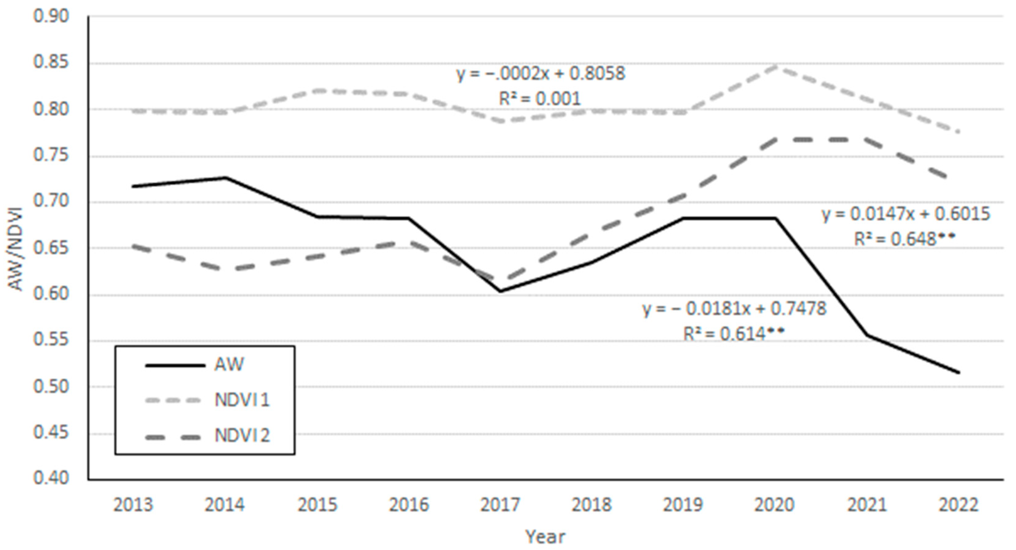
The meteorology of the study area shows a clear trend towards drier conditions during the examined 10-year period, which is reflected in a highly significant decrease in the AW scalar (Figure 2). This trend is induced by a combination of meteorological factors. Annual rainfall is, in fact, irregularly decreasing (from over 1000 to around 700 mm), while annual PET is slightly increasing (from about 1200 to 1300 mm), due to quite regular temperature and radiation rises.
This trend has a marginal impact on the NDVI of the umbrella pine stand (NDVI 1), which is moderately correlated with AW (Table 1) and only marginally decreasing. In contrast, increasing dryness is nearly uninfluential on the NDVI of the regrowing maritime pine stand (NDVI 2), which is negatively correlated with AW and shows a highly significant rise (Table 1; Figure 2). The influence of dryness on this stand is reflected only by the NDVI drops coincident with the main AW decreases (e.g., in 2017 and 2022).
These patterns have clear consequences on the GPP predicted by the two models considered, which, as previously noted, work using different principles and drivers. BIOME-BGC, in fact, being parameterized and driven in the same way for both pine species, provides the same estimates for the two stands. In contrast, C-Fix, which is mostly driven by the NDVI of the two stands, yields diversified predictions.
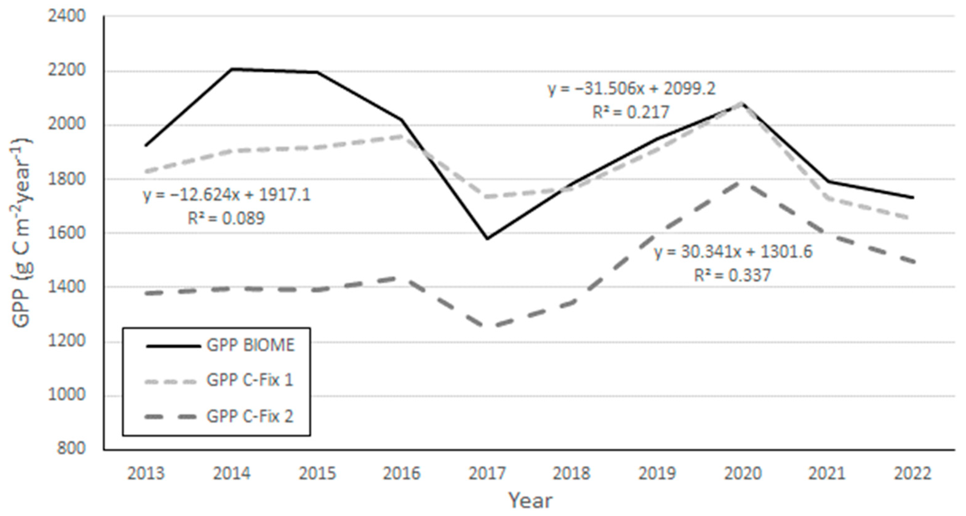
This is visible in Figure 3: the GPP simulated by BIOME-BGC is close to that predicted by C-Fix for the umbrella pine stand (around 1900–2000 g C m−2 year−1) and follows a similar decreasing trend. The GPP predicted by C-Fix for the maritime pine stand is instead lower but increases following the respective NDVI rise. The correlations in Table 1 confirm these patterns, particularly concerning the low accordance between NDVI 2 and the GPP of BIOME-BGC and, above all, C-Fix 1.
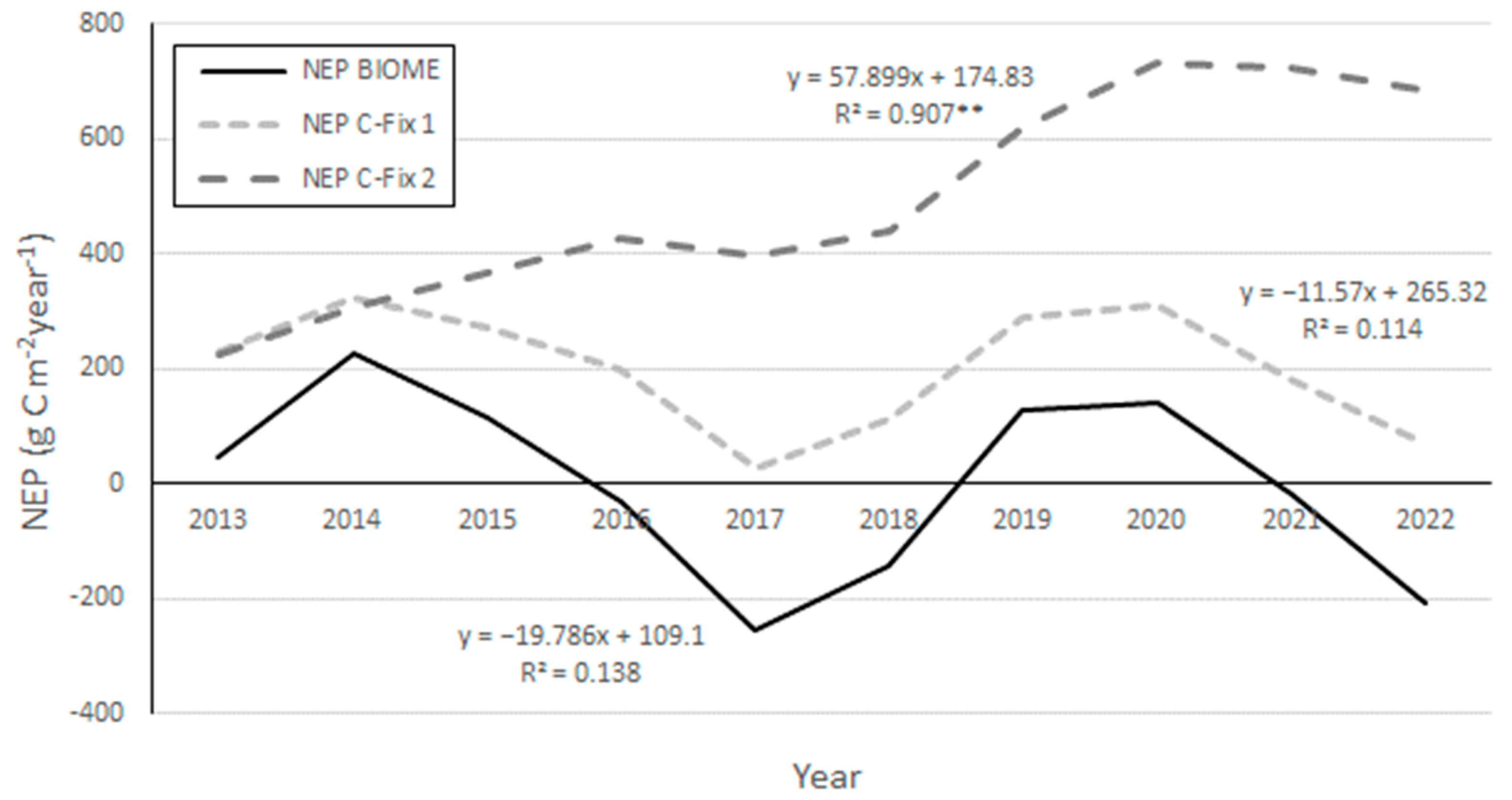
Finally, Figure 4 shows the NEP trends simulated as described above for the two stands. In accordance with the theoretical foundation of the model, the NEP simulated by BIOME-BGC is, on average, very close to 0 g C m−2 year−1 and shows a slightly decreasing trend.
The case is different when applying the model combination, which is also driven by the three scalars of Equation (3). The vegetation scalars (NV and FC) obtained from the processing of the LiDAR data for the umbrella pine stand are descriptive of a mature forest (NV = 0.60 and FC = 0.72); the NS derived from the corrected SOC of the Tuscany map is typical of a similar ecosystem condition (0.59). The NEP simulated by the model combination using this setting follows a trend that is almost parallel to that of BIOME-BGC but is always positive around 200 g C m−2 year−1.
A different NEP evolution is predicted by the model combination for the regrowing maritime pine stand. In this case, in fact, FC rises from around 0.4 to 0.8 and NV increases from about 0.04 to 0.11. Following these trends and that of GPP C-Fix 2, the simulated NEP increases almost linearly from around 200 to over 600 g C m−2 year−1.
Again, Table 1 provides insights on the correlations between NEP and the other variables. The NEP series simulated by BIOME-BGC and by the model combination for the umbrella pine stand is highly dependent on the AW meteorological scalar, as well as on the respective GPP estimates. The NEP simulated by the model combination for the maritime pine stand instead shows a negative correlation with most other variables and a highly significant positive correlation only with NDVI 2 and GPP C-Fix 2.

4. Discussion and Conclusions

The current study is based on the consolidated capacity of Modified C-Fix to predict forest GPP in Mediterranean areas, which has been demonstrated in previous investigations [7,15]. A similar capability has been proven for the calibrated BIOME-BGC versions to simulate all forest processes in the same region [19]. Further investigations have supported the efficiency of the model combination for predicting the actual processes of forest ecosystems in different development phases [13]. In particular, the independent estimation of the three C pools, which regulate photosynthesis, autotrophic and heterotrophic respirations, permits an efficient simulation of the processes of ecosystems far from equilibrium conditions [20].
Owing to these properties, the strategy can be adapted to analyzing the impacts of both natural factors and human-induced disturbances. A first example of this possibility has been currently illustrated for a Mediterranean coastal area covered by two pine forest ecosystems in different development phases. The results obtained show that the first stand, representative of an old-growth forest, is mostly controlled by meteorology, i.e., by the increasing dryness of the area, which induces slightly decreasing GPP and NEP trends. In accordance with the forest equilibrium theory adopted by the model combination strategy, the GPP of this stand is quite high, while the NEP is moderate.
The second stand, representative of a secondary succession after clearcuts, partly counteracts the influence of increasing dryness by a rapid regrowing, which induces significant increases in NDVI and simulated GPP. This evolution is accompanied by an intense biomass accumulation which is typical of the initial phase of a secondary succession. Still in accordance with the mentioned equilibrium theory, the simulation of the stand NEP takes into consideration this evolution through the progressive increase in the two vegetation scalars (NV and FC). The modeling exercise finally results in clear rises of simulated NEP and C stock.
A direct validation of the GPP and NEP estimates obtained by the model combination is not presently feasible due to the lack of ground observations taken during the ten years examined. The mean values of both these variables, however, are comparable to those measured by an eddy covariance flux tower, which was active in an adjacent maritime pine stand during the period 2001–2005. This stand was representative of a relatively mature (60–70 years old) but not fully stocked forest, where woody biomass was still accumulating. The average values of GPP and NEP observed by that tower were around 1600–1800 and 400–500 g C m−2 year−1, respectively [19]. The lower NEP currently simulated for the first, mature stand can be reasonably attributed to its smallest distance from equilibrium (fully stocked) condition. The higher net C flux predicted for the second stand in the last years can instead be attributed to the respective intensive biomass accumulation phase.
These patterns are in accordance with the variations of woody biomass which have been observed on the ground during the study decade. No significant change in GSV has, in fact, been detected by the forest managers in the umbrella pine stand (personal communication with F. Logli, Regional Park Authority). In contrast, the storage of woody biomass which accompanies the NEP evolution simulated for the maritime pine stand is testified to by the increasing tree canopy density and height observable in situ. The mean canopy height of this stand, in fact, rose from nearly 0 m in 2013 to 3–4 m in 2023.
The results of the described experiment are affected by several sources of uncertainty. In addition to the limits of the modeling background, discussed in previous publications [7,15], the use of interpolated and remotely sensed input datasets induces inaccuracies that cannot be presently quantified. In particular, the utilization of a unique weather dataset to guide all modeling exercises introduces a spurious component into most of the statistical relationships found between the input and output data series. The simulation strategy applied, however, also takes into account major forest attributes which counteract the impact of meteorology (i.e., the NDVI and vegetation scalars), thus providing information which is partly independent of this.
The datasets utilized are differently capable of describing the main ecosystem features regulating gross and net C fluxes. The spatiotemporal variability of meteorology in the flat study area is presumably reproduced well by the interpolated weather dataset. The same, however, is not fully the case for the MODIS NDVI imagery, which has a spatial resolution insufficient to capture the fine spatial details of the examined stands [21]. The uncertainty of the simulation process could therefore be reduced by the use of higher spatial resolution images such as those taken by Landsat TM/ETM+/OLI and Sentinel-2 MSI. The use of NDVI imagery taken by these sensors in the current case, however, is hampered by issues of temporal resolution and coverage, respectively [22,23]. A similar problem affects the SOC map utilized, which has the finest spatial resolution (250 m) allowed by the soil mapping technologies applicable at the regional scale [24]. The issues induced by the use of low spatial resolution datasets are, in any case, mitigated by the combination with aircraft LiDAR observations, which can properly predict the scalars related to static vegetation properties (FC and NV).
In summary, the current investigation has illustrated the potential of the proposed model combination strategy to quantify the different C accumulation capacities of forests subjected to the same meteorological constraints but in diverging development phases due to different human controls. Such assessment is relevant for providing the information required for sustainable forest management, concerning, in particular, ecosystem services linked to the C cycle.
The potential of the strategy, however, should be confirmed by future investigations carried out using more complete ground and remote sensing observations of C fluxes and stocks taken in the same and other forest areas. These investigations could also consider different methods to integrate remotely sensed GPP estimates with models of ecosystem processes that take into account the actual forest structure and development phase.

Author Contributions

Conceptualization, F.M. and M.C.; methodology, L.F.; investigation, M.C. and S.V.; data curation, L.F.; writing—original draft preparation, M.C.; writing—review and editing, F.M. and S.V.; supervision, F.M. All authors have read and agreed to the published version of the manuscript.

Funding

This research received no external funding.

Data Availability Statement

Data cited in this manuscript are available in registries that are freely accessible to the public (https://modis.gsfc.nasa.gov, last accessed on 10 September 2023).

Acknowledgments

The authors want to thank L. Bottai (LaMMA Consortium) for providing a preprocessed version of the utilized LiDAR dataset and F. Logli (San Rossore Regional Park Authority) for providing forestry information on the study area. The authors wish to thank three anonymous RS reviewers for their helpful comments which improved the quality of the original manuscript.

Conflicts of Interest

The authors declare no conflicts of interest.

References

  1. Waring, H.R.; Running, S.W. Forest Ecosystems. In Analysis at Multiples Scales, 3rd ed.; Academic Press: San Diego, CA, USA, 2007. [Google Scholar]
  2. Pan, Y.; Birdsey, R.A.; Fang, J.; Houghton, R.; Kauppi, P.E.; Kurz, W.A.; Phillips, O.L.; Shvidenko, A.; Lewis, S.L.; Canadell, J.G.; et al. A large and persistent carbon sink in the world’s forests. Science 2011, 333, 988–993. [Google Scholar] [CrossRef]
  3. Su, Y.; Zhang, W.; Liu, B.; Tian, X.; Chen, S.; Wang, H.; Mao, Y. Forest carbon flux simulation using multi-source data and incorporation of remotely sensed model with process-based model. Remote Sens. 2022, 14, 4766. [Google Scholar] [CrossRef]
  4. Yan, M.; Tian, X.; Li, Z.; Chen, E.; Wang, X.; Han, Z.; Sun, H. Simulation of forest carbon fluxes using model incorporation and data assimilation. Remote Sens. 2016, 8, 567. [Google Scholar] [CrossRef]
  5. Zhao, J.; Lu, D.; Cao, Y.; Zhang, L.; Peng, H.; Wang, K.; Xi, H.; Wang, C. An integrated remote sensing and model approach for assessing forest carbon fluxes in China. Sci. Total Environ. 2022, 811, 152480. [Google Scholar] [CrossRef]
  6. Srinet, R.; Nandy, S.; Patel, N.R.; Padalia, H.; Watham, T.; Singh, S.K.; Chauhan, P. Simulation of forest carbon fluxes by integrating remote sensing data into biome-BGC model. Ecol. Model. 2023, 475, 110185. [Google Scholar] [CrossRef]
  7. Maselli, F.; Chiesi, M.; Moriondo, M.; Fibbi, L.; Bindi, M.; Running, S.W. Modelling the forest carbon budget of a Mediterranean region through the integration of ground and satellite data. Ecol. Model. 2009, 220, 330–342. [Google Scholar] [CrossRef]
  8. Fibbi, L.; Moriondo, M.; Chiesi, M.; Bindi, M.; Maselli, F. Impacts of climate changes on the gross primary production of Italian forests. Ann. For. Sci. 2019, 76, 59. [Google Scholar] [CrossRef]
  9. Sciarretta, A.; Marziali, L.; Squarcini, M.; Marianelli, L.; Benassai, D.; Logli, F.; Roversi, P.F. Adaptive management of invasive pests in natural protected areas: The case of Matsucoccus feytaudi in Central Italy. Bull. Entomol. Res. 2015, 106, 9–18. [Google Scholar] [CrossRef]
  10. Thornton, P.E.; Running, S.W.; White, M.A. Generating surfaces of daily meteorological variables over large regions of complex terrain. J. Hydrol. 1997, 190, 214–251. [Google Scholar] [CrossRef]
  11. Thornton, P.E.; Hasenauer, H.; White, M.A. Simultaneous estimation of daily solar radiation and humidity from observed temperature and precipitation: An application over complex terrain in Austria. Agric. For. Meteorol. 2000, 104, 255–271. [Google Scholar] [CrossRef]
  12. Gardin, L.; Chiesi, M.; Fibbi, L.; Maselli, F. Mapping soil organic carbon in Tuscany through the statistical combination of ground observations with ancillary and remote sensing data. Geoderma 2021, 404, 115386. [Google Scholar] [CrossRef]
  13. Chirici, G.; Chiesi, M.; Corona, P.; Puletti, N.; Mura, M.; Maselli, F. Prediction of forest NPP in Italy by the combination of ground and remote sensing data. Eur. J. For. Res. 2015, 134, 453–467. [Google Scholar] [CrossRef]
  14. Veroustraete, F.; Sabbe, H.; Eerens, H. Estimation of carbon mass fluxes over Europe using the C-Fix model and Euroflux data. Remote Sens. Environ. 2002, 83, 376–399. [Google Scholar] [CrossRef]
  15. Maselli, F.; Papale, D.; Puletti, N.; Chirici, G.; Corona, P. Combining remote sensing and ancillary data to monitor the gross productivity of water-limited forest ecosystems. Remote Sens. Environ. 2009, 113, 657–667. [Google Scholar] [CrossRef]
  16. Golinkoff, J. Biome BGC Version 4.2: Theoretical Framework of Biome-BGC. January 2010. Available online: http://www.ntsg.umt.edu/project/biome-bgc (accessed on 14 March 2023).
  17. White, M.A.; Thornton, P.E.; Running, S.W.; Nemani, R.R. Parameterization and sensitivity analysis of the BIOME-BGC terrestrial ecosystem model: Net primary production controls. Earth Interact. 2000, 4, 1–85. [Google Scholar] [CrossRef]
  18. Liu, S.; Bond-Lamberty, B.; Hicke, J.A.; Vargas, R.; Zhao, S.; Chen, J.; Edburg, S.L.; Hu, Y.; Liu, J.; McGuire, A.D.; et al. Simulating the impacts of disturbances on forest carbon cycling in North America: Processes, data, models, and challenges. J. Geophys. Res. Biogeoscience 2011, 116, G00K08. [Google Scholar] [CrossRef]
  19. Chirici, G.; Chiesi, M.; Fibbi, L.; Giannetti, F.; Corona, P.; Maselli, F. High spatial resolution modelling of net forest carbon fluxes based on ground and remote sensing data. Agric. For. Meteorol. 2022, 316, 108866. [Google Scholar] [CrossRef]
  20. Maselli, F.; Mari, R.; Chiesi, M. Use of LiDAR data to simulate forest net primary production. Int. J. Remote Sens. 2013, 34, 2487–2501. [Google Scholar] [CrossRef]
  21. Heute, A.; Didan, K.; Miura, T.; Rodriguez, E.P.; Gao, X.; Ferreira, L.G. Overview of the radiometric and biophysical performance of the MODIS vegetation indices. Remote Sens. Environ. 2002, 83, 195–213. [Google Scholar] [CrossRef]
  22. Ju, J.; Roy, D.P. The availability of cloud-free Landsat ETM+ data over the conterminous United States and globally. Remote Sens. Environ. 2008, 112, 1196–1211. [Google Scholar] [CrossRef]
  23. Wu, J.; Lin, L.; Li, T.; Cheng, Q.; Zhang, C.; Shen, H. Fusing Landsat 8 and Sentinel-2 data for 10-m dense time-series imagery using a degradation-term constrained deep network. Int. J. Appl. Earth Obs. Geoinf. 2022, 108, 102738. [Google Scholar] [CrossRef]
  24. Pouladi, N.; Gholizadeh, A.; Khosrawi, V.; Boruvka, L. Digital mapping of soil organic carbon using remote sensing data: A systematic review. Catena 2023, 232, 107409. [Google Scholar] [CrossRef]
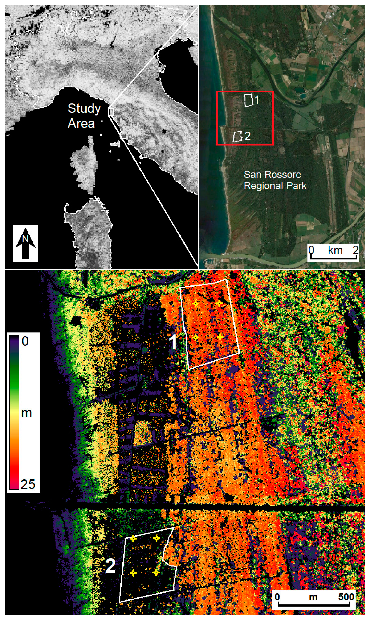
Figure 1. Top-left: MODIS NDVI image from August 2015 (from 0 = black to 1 = white) showing the position of the study area in Central Italy. Top-right: Google Earth image from 28 August 2015 showing the San Rossore Regional Park and the stands covered by P. pinea (1) and P. pinaster (2) (white lines). The area circumscribed by the red box is enlarged in the bottom image, which shows the same stands (white lines) and the centers of the respective MODIS pixels (yellow crosses) superimposed on the CHM obtained from the LiDAR acquisition of 2015 (see text for details).
Remotesensing 16 00232 g001
Figure 2. Trends of the meteorological water stress scalar (AW) and of the NDVI from the two stands during the study period. The equations refer to the respective linear regressions towards sequential years from 2013 to 2022 (** = highly significant correlation, p < 0.01).
Remotesensing 16 00232 g002
Figure 3. Trends of GPP simulated by BIOME-BGC and by C-Fix for the two stands during the study period. The equations refer to the respective linear regressions towards sequential years from 2013 to 2022.
Remotesensing 16 00232 g003
Figure 4. Trends of NEP simulated by BIOME-BGC and by C-Fix for the two stands during the study period. The equations refer to the respective linear regressions towards sequential years from 2013 to 2022 (** = highly significant correlation, p < 0.01).
Remotesensing 16 00232 g004
Table 1. Correlations found between all considered variables during the ten study years (2013–2022) (* = significant correlation, p < 0.05; ** = highly significant correlation, p < 0.01).
NDVI 1NDVI 2GPP
BIOME
GPP
C-Fix 1
GPP
C-Fix 2
NEP
BIOME
NEP
C-Fix 1
NEP
C-Fix 2
AW0.410 *−0.427 *0.744 **0.769 **−0.0320.744 **0.755 **−0.600 **
NDVI 1 0.3640.562 *0.799 **0.585 *0.519 *0.584 **0.210
NDVI 2 0.3320.0630.887 **0.0880.1370.906 **
GPP BIOME 0.778 **0.2820.900 **0.904 **−0.236
GPP C-Fix 1 0.484 *0.750 **0.808 **−0.035
GPP C-Fix 2 0.444 *0.503 *0.787 **
NEP BIOME 0.993 **−0.109
NEP C-Fix 1 −0.064
Disclaimer/Publisher’s Note: The statements, opinions and data contained in all publications are solely those of the individual author(s) and contributor(s) and not of MDPI and/or the editor(s). MDPI and/or the editor(s) disclaim responsibility for any injury to people or property resulting from any ideas, methods, instructions or products referred to in the content.