A FEM Flow Impact Acoustic Model Applied to Rapid Computation of Ocean-Acoustic Remote Sensing in Mesoscale Eddy Seas

Abstract

Mesoscale eddies have an impact on the marine environment mainly in two areas, namely, currents and changes in the sound velocity gradient due to temperature and salt stirring. The traditional underwater-related remote sensing acoustic remote sensing model is capable of analyzing the acoustic field under the change in sound velocity gradient, but it is not capable of analyzing the acoustic field under the influence of ocean currents. In order to more effectively analyze the changes in the acoustic field caused by mesoscale eddies, this paper proposes a FEM flow impact model applied to the rapid computation of acoustic remote sensing of mesoscale eddies in the sea area. The algorithm first performs a grid optimization of the sea area model based on vertical sound velocity variations and completes the classification of sound velocity layer junctions. At the same time, we construct the sound velocity gradient environment affected by the mesoscale eddy and then simplify the fluid flow in the mesoscale eddy into a non-viscous and non-rotating velocity potential, and then participate in the solution of the three-dimensional spatial fluctuation equations in the form of time-harmonic in the frequency domain, from which we can obtain the truncated sound pressure as well as the propagation loss, and quickly and completely characterize the acoustic remote sensing of the sea area of the mesoscale eddy. The paper verifies the effectiveness of the algorithm through SW06-contained flow experiments and further proposes an optimization formula for sound velocity inversion. We analyze this using measured data of mesoscale eddy fields in the Bering Sea waters during 2022 and find that eddies have a greater effect on the propagation of the acoustic field along their flow direction.

1. Introduction

Mesoscale oceanic eddies, as one of the most typical oceanic phenomena, have a wide range of impacts on the transportation of marine materials, the safety of ship navigation, and climate change [1,2,3]. 2023 Volkov et al. The effect of mesoscale eddies on ocean-acoustic remote sensing is summarized in two main points. One is the change in the vertical sound velocity gradient due to the churning of temperature and salt from the surface to the depths of the sea [4,5], and the other is the unsteady currents at the edges of mesoscale eddies [6].

In the last decade, ocean-acoustic remote sensing has been trying to use acoustic models to better analyze the effects of mesoscale eddies on acoustic propagation, and the most common models usually include simple normal wave models [7], parabolic equation models [8], fast field models [9], ray models [10], etc. These models are based on a certain simplification of the actual problem and are obtained by making a reasonable approximation to the solution of the fluctuation equations. Different approximation conditions have led conventional acoustic models to focus only on solving the sound field under specific environmental conditions. For example, simple normal wave models are often modeled using “adiabatic approximation” or “mode coupling” treatments, which are often applied to the construction of accurate acoustic fields without energy exchange or at low speeds. The ray model is based on the fact that high-frequency sound waves can be approximated as sound lines, and is applied to the problem of propagation of high-frequency sound sources. The fast field model directly solves the integral expression for the sound field at each layer and is applied to solve the sound field results from mesoscale eddies in a distance-independent environment. These models often complete the analysis of the acoustic impact of mesoscale eddies by calculating the change in sound velocity gradient due to vertical thermohaline churning through a horizontally layered structure, but these traditional methods, due to the presence of no-flow background field assumptions [11], are therefore unable to solve the problem of mesoscale eddy flow fields. This leads to a large error between the computed and measured results of the mesoscale eddy presence sea area models, so the traditional model cannot completely analyze the ocean-acoustic remote sensing characteristics of mesoscale eddy seas [12,13,14].

With the wide application of finite element computational models in ocean computation [15], the use of finite element methods to solve the acoustic field has become a new direction, which makes it possible to solve the effect of unsteady currents at the edges of mesoscale eddies on ocean-acoustic remote sensing. The solution idea of the finite element computational model is to disassemble the physical domain into multiple sub-domains and solve the approximate solutions as well as the exact solutions within the multiple sub-domains with a finite number of degrees of freedom. The complex solution domain is simplified by coupling the various subdomains to be solved through the continuity of the boundary. Such a solution allows finite element models to construct complex environmental fields in mesoscale eddy seas [16,17]. Compared with the traditional model, the solution of the finite element model is a dimensional reduction of the acoustic computational equations, and the results of numerous studies have shown that the simulation accuracy of the finite element model is superior to that of the traditional model [18,19,20,21]. In 2021, Zichen Wang et al. [22] constructed a finite element model based on the convective fluctuation equation for acoustic wave propagation in the presence of background currents and initially reached the conditions for analyzing the effect of the flow field on the acoustic field, which made it possible to analyze the flow-influenced ocean-acoustic remote sensing in mesoscale eddy seas. However, the convective fluctuation equations need to be discretized in both the spatial and temporal domains, which requires very high computational performance, and the sea area affected by mesoscale eddies in practice usually covers more than 30 km [23]. Therefore, it is difficult to do fast calculations and analysis of 3D sound fields. The current calculation of the 3D acoustic field in mesoscale eddy seas realized by the finite element method is still in the no-flow state or multi-model coupling [24,25], which is not able to completely analyze the variation of the acoustic field in mesoscale eddy seas.

In order to more completely, efficiently, and rapidly analyze the sound field changes due to mesoscale eddies, in this paper, we propose a FEM flow impact model applied to the rapid computation of acoustic remote sensing in mesoscale eddy seas, simultaneously addressing the effects of sound velocity gradients and currents on ocean acoustic remote sensing in mesoscale eddy seas. The algorithm first performs the mesh optimization of the sea area model based on the vertical sound velocity change and completes the sound velocity layer junction classification according to the curvature region maximum detection method of the endpoints of the acoustic layer spectral peaks. Taking the average propagation loss error accuracy of 3 dB as the limit, the critical grid size of the grid optimization model is gradually approximated, and the optimized model can save more than 98% of the computation time, which greatly improves the computation speed. The model is then used to construct a mesoscale eddy-influenced sound velocity gradient environment. The model-solving process describes the acoustic field in the form of time harmonics on the basis of the 3D convective fluctuation equations, which transform the convective fluctuation equations in the time domain into the convective Helmholtz equations in the frequency domain [26], improving the computational speed. Meanwhile, under the premise that the sound source is a small-amplitude wave, the linear Euler equations are obtained by neglecting the nonlinear effects in the convective Helmholtz equations [27], and the fluid flow brought about by the mesoscale vortices is reduced to a nonviscous, non-rotating velocity potential by referring to the simplifications in aerodynamic acoustics [28,29,30].

In this paper, the correctness of the model is verified using the analytical solution, and the results of forward and backward applications of the model are analyzed. In the forward application, we analyze the results of the model according to the characteristics of the Bering Sea region, which is characterized by the occurrence of many eddies and the complexity and strength of the current field [31,32], and identify and select one of the cold eddies for analysis based on the no-threshold contour method [33]. It is found that vortices have a greater effect on the propagation of the acoustic field along their flow direction, and the effect on the acoustic field offset can be up to 3.5 m at a range of 10 km, and the effect on the propagation loss error can be up to 1 dB or greater. In the inverse application, we analyze the model calculations and inversely perform the regional sound velocity according to the Prony method [34], and further propose an optimization formula for the sound velocity inversion with the feature that the model can calculate the effect of the flow velocity on the acoustic field, which eliminates the effect of the flow velocity. The paper inverts the structure of the acoustic velocity gradient through the heavily instrumented Environmental Moorings data from the SW06 contained flow experiment [35,36], verifying the accuracy of the model used for the inversion and the effectiveness of the optimization algorithm.

The article structure of this paper is organized as follows: Section 1 is the Introduction, which summarizes the results of previous research and the main ideas of the article. Section 2, Materials and Methods, focuses on a detailed description of the dataset and the principles of model construction. Section 3, Results, provides the results of the validation of the model against the analytical solution while applying the model to perform forward eddy analysis and reverse flow inversion. Section 4 is the Discussion, which includes the analysis of the results of model optimization, eddy sound field, and flow inversion. Section 5 summarizes the whole paper.

2. Materials and Methods

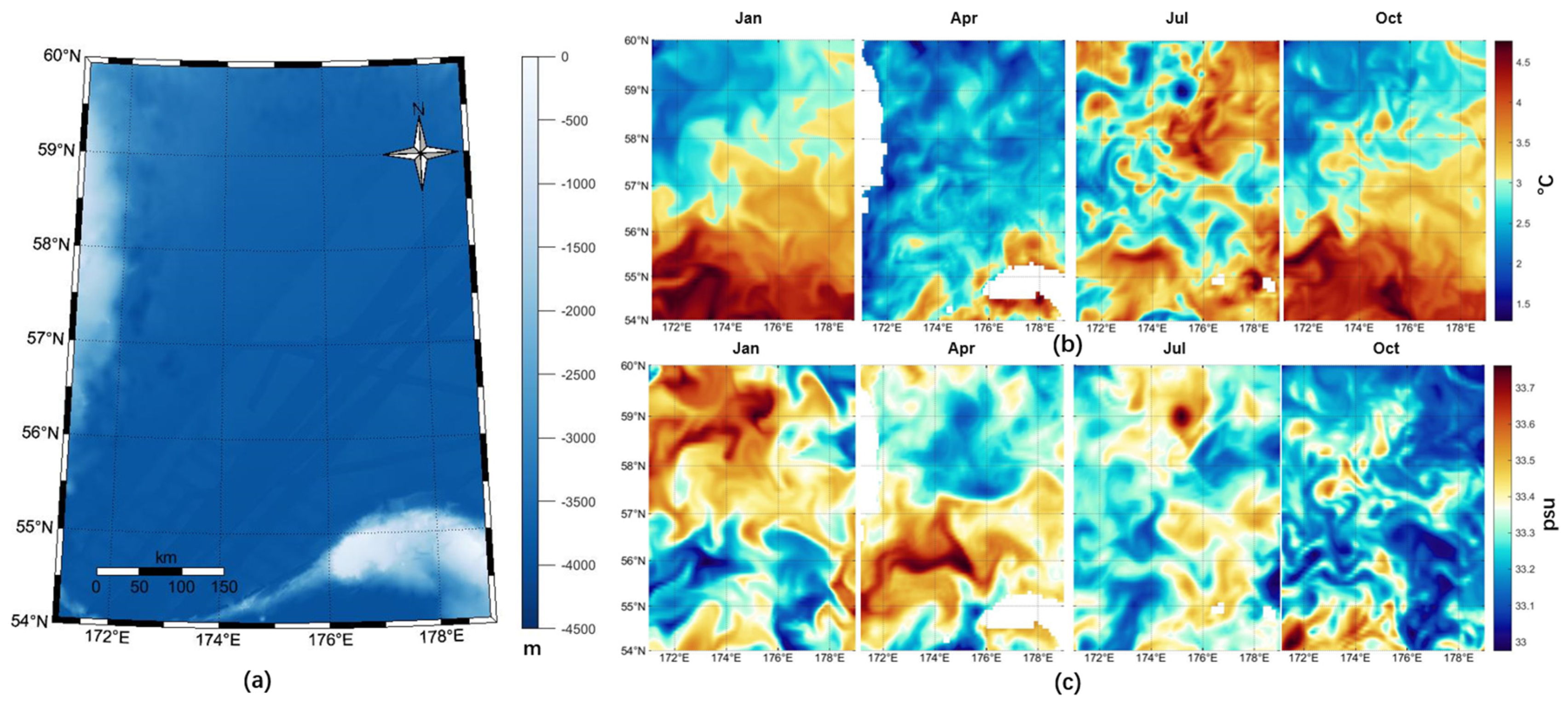
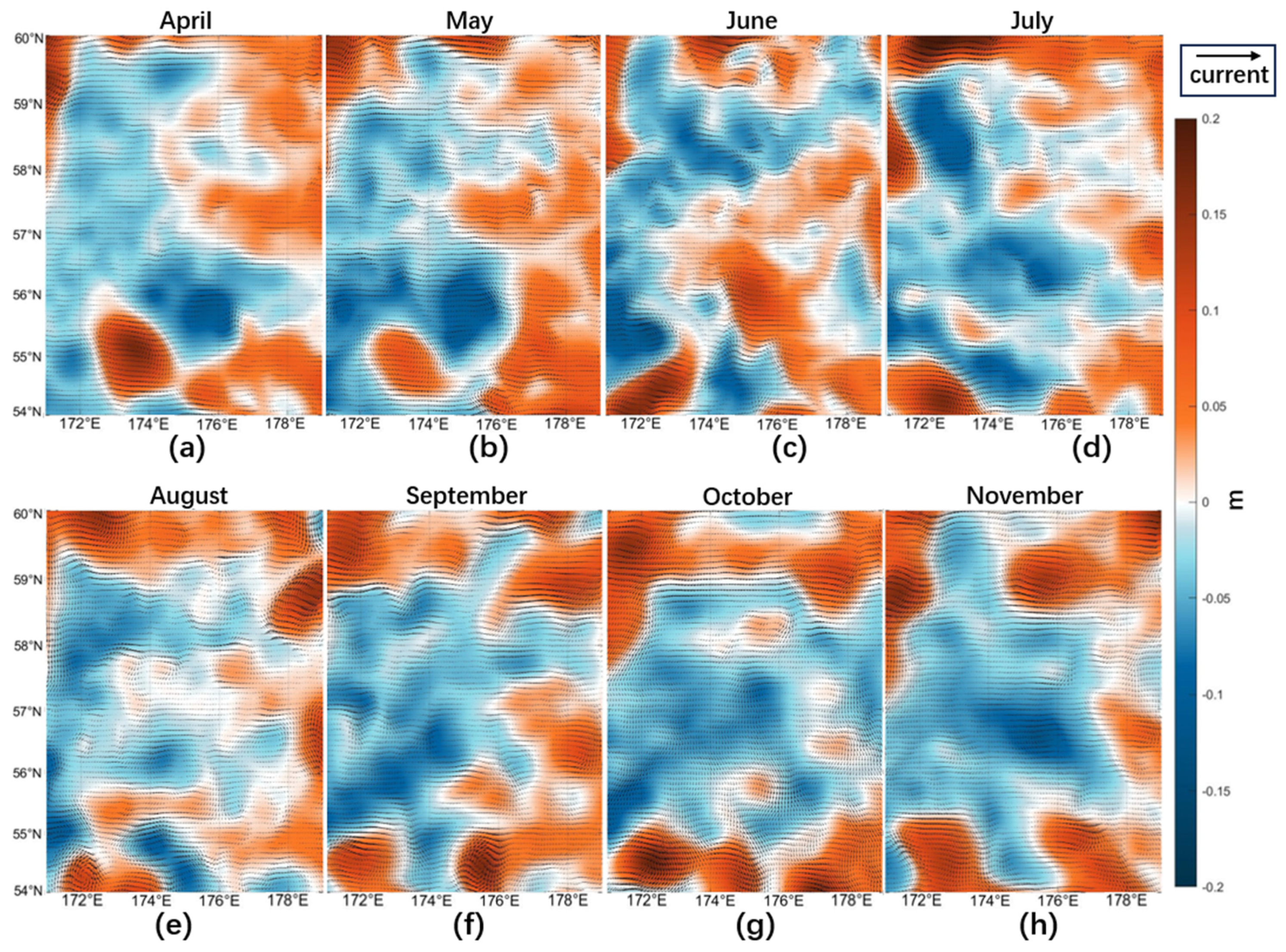
2.1. Satellite Remote Sensing Data

The Bering Sea region studied in the article is located in the North Pacific Ocean, surrounded by the Alaskan Peninsula and the Aleutian Islands, with a range of seawater depths as shown in Figure 1a. The composition of currents in the region consists mainly of the following: the North Aleutian Landward Slope Current (NALC), which flows northeastward off the coast of Alaska; the Bering Sea Slope Current (BSSC), which splits from the NALC as it flows in the interior of the Bering Sea; and the Westerly Drift Current (WDC), which passes through the Bering Strait and enters the North Atlantic Ocean from the North Atlantic Ocean into the North Pacific Ocean. Hydrodynamic studies of the region have shown that the surface water circulation in the Bering Sea region is distinctly seasonal and that the eddies generated as a result of the water circulation are also seasonal, with a large number of anticyclones generated by currents flowing southwestward along the land slope in January and cyclone formation influenced by northeasterly-flowing currents in July [37]. The abundance of eddies also facilitates the study of sound field modeling under the influence of eddies.

The data in this article is from Copernicus Marine Service [38,39,40], the platform that is part of the European Copernicus program, which provides a wide range of data for ocean analysis, including ocean currents, temperature, salinity, chlorophyll content, and many other oceanographic data. The paper uses part of the Global Ocean Physics Analysis and Forecast dataset in the range 54°N–60°N, 171°E–179°E, which consists of combined measurements from several satellite altimeters (PT6H-i, P1D-m, P1M-m, PT1H-m, PT1H-i). The horizontal dataset can reach 1/12 degree, and the vertical depth layer consists of 50 unequally spaced layers from 0 m to 5500 m, with a rich variety of data containing daily mean temperature, salinity, the velocity of flow, and sea surface height at each grid point, which can meet the needs of eddy identification and model construction at the same time. Among them, the deepest depth of the Bering Sea region selected for the study reaches 4500 m.

Among them, the temperature and salinity measured by satellite remote sensing will have large variations with seasonal and flow field changes, as shown in Figure 1b,c, and the high-resolution temperature-salinity and flow velocity data are conducive to remotely sensing-related acoustic field model construction.

2.2. Finite Element Linear Potential Flow Principle

The basic idea of the finite element method is to divide the complex physical field into several small and simple, through the continuity of the coupling between the units to solve, through the separate calculation of the solution of each unit, and then get the solution of the whole physical field. When dealing with higher-order partial differential equations via the finite element method, they are usually transformed into integral equations expressed in a weak form in order to realize the solution of the equations in the case of a complex ocean boundary.

Linear potential flow theory is a theory that simplifies fluid flow to a linear, inviscid, positive-pressure, spinless flow and is a simplification of the hydrodynamic problem. Linear potential flow theory can be solved using the finite element method by dividing the complex computational domain into a finite number of small cells and applying appropriate mathematical theories and approximations to each of them to obtain a discretized system of equations. These discretized equations can be computed numerically to obtain an approximate solution for the sound field. The effect of mesoscale eddies on the sound field can be partially described using a finite element model of linear potential flow theory.

The linearized Euler equations for the fluid are shown below [41]:

$$\frac{\partial {\rho }_t}{\partial t}+\nabla ·\left({\rho }_t{u}_0+{\rho }_0{u}_t\right)=M$$

(1)

$$\rho \frac{D{u}_t}{Dt}+\left(\left[u_t+\frac{{\rho }_t}{{\rho }_0}{u}_0\right]·\nabla \right)u_0+\left(u_0·\nabla \right)u_t+\frac{1}{{\rho }_0}\nabla p_t=\frac{1}{{\rho }_0}(F-u_{0}M)$$

(2)

$$\frac{\partial p_t}{\partial t}+u_t·\nabla p_0+p_t\gamma \left(\nabla ·u_0\right)+u_0·\nabla p_t+\gamma p_0(\nabla ·u_t)=\left(\gamma -1\right)\mathrm{Q}+\frac{\gamma p_0}{{\rho }_0}M$$

(3)

where the velocity field is $u$, the temperature is $T$, the density is $\rho$, $p$ denotes the pressure, $\gamma$ denotes the adiabatic index, and the M, F, and Q are the source terms.

Using the mass conservation equation, express $\frac{\partial {\rho }_t}{\partial t}$ as $-{\rho }_0\nabla ·u_t$ and substituting into (1), the following equation is obtained by collapsing:

$$\nabla ·\left({\rho }_t{u}_0+{\rho }_0{u}_t\right)=M$$

(4)

obtained by acoustic approximation:

$$\frac{\partial p}{\partial \rho }{I}_0=c_0^2$$

(5)

$$u_t=V+\nabla \mathsf{\Phi }$$

(6)

where $c_0$ is the speed of sound, Vis the fluid velocity field, and $\mathsf{\Phi }$ is the velocity potential function, which can be obtained by substituting (5), (6) into (2) and neglecting higher order terms.

$$\rho \frac{DV}{Dt}+\left(\left[V+\frac{{\rho }_t}{{\rho }_0}{u}_0\right]·\nabla \right)u_0+\left(u_0·\nabla \right)V+\left(u_0·\nabla \right)\nabla \mathsf{\Phi }+\frac{1}{{\rho }_0\nabla p_t}=\frac{1}{{\rho }_0}(F-u_{0}M)$$

(7)

The $\rho \frac{DV}{Dt}$ denotes the material derivative of the density multiplied by the velocity, and is an extra term due to the approximation of higher order terms.

Next, the sum of the two equations is obtained by substituting (5) and (6) into (3) to obtain the Linearized Potential Flow equation:

$$-\frac{{\rho }_0}{c_0^2}\frac{\partial }{\partial t}\left(\frac{\partial \mathsf{\Phi }}{\partial t}+V·\nabla \mathsf{\Phi }\right)+\nabla ·\left[{\rho }_0\nabla \mathsf{\Phi }-\frac{{\rho }_0}{c_0^2}\left(\frac{\partial \mathsf{\Phi }}{\partial t}+V·\nabla \mathsf{\Phi }\right)V\right]=0$$

(8)

The $\rho$ in this equation is the time-independent part. The corresponding acoustic part is $\rho \left(r,t\right)=\frac{p\left(r,t\right)}{c_0^2}$, where p is the sound pressure, given by the following equation:

$$p\left(r,t\right)=-{\rho }_0(\frac{\partial \mathsf{\Phi }}{\partial t}+V·\nabla \mathsf{\Phi })$$

(9)

Afterward, the solution of the equations under the finite element method is derived, and since a finite element frequency domain model is constructed, it is necessary to discretize the time domain and introduce frequency transformations.

First, the time domain is partitioned into discrete time steps, denoted as $\mathsf{\Delta }\mathrm{t}$.

The differential approximation of the velocity potential function, $\mathsf{\Phi },$ and the fluid velocity field, V, is as follows:

$$\frac{{\partial }^2\mathsf{\Phi }}{\partial t^2}\approx ({\mathsf{\Phi }}_{n+1}-2{\mathsf{\Phi }}_n+{\mathsf{\Phi }}_{n-1})/\mathsf{\Delta }{\mathrm{t}}^2$$

(10)

$$V_{n+1}\approx ({\mathrm{V}}_{n+1}-V_n)/\mathsf{\Delta }\mathrm{t}$$

(11)

The frequency transformations of the velocity potential and the flow field are subsequently obtained in terms of $\mathsf{\Phi }\left(\mathsf{\omega }\right)$ and $\mathrm{V}\left(\mathsf{\omega }\right)$, respectively.

$$\frac{{\partial }^2\mathsf{\Phi }}{\partial t^2}\approx (\mathsf{\Phi }(\mathsf{\omega })-2{\mathsf{\Phi }}_n+{\mathsf{\Phi }}_{n-1})/\mathsf{\Delta }{\mathrm{t}}^2$$

(12)

$$V_{n+1}\approx \left(\mathrm{V}\right(\mathsf{\omega })-V_n)/\mathsf{\Delta }\mathrm{t}$$

(13)

The frequency-transformed velocity potential function $\mathsf{\Phi }\left(\mathsf{\omega }\right)$ and the fluid velocity field $\mathrm{V}\left(\mathsf{\omega }\right)$ are expressed as a linear combination of shape functions.

$$\mathsf{\Phi }\left(\mathsf{\omega }\right)=\sum \left(Ni{\mathsf{\Phi }}_i\right(\mathsf{\omega }\left)\right)$$

(14)

$$\mathrm{V}\left(\mathsf{\omega }\right)=\sum \left(Ni{\mathrm{V}}_i\right(\mathsf{\omega }\left)\right)$$

(15)

where $Ni$ is the shape function at node $i$.

For the weak form, one can multiply both sides of Equation (8) by a test function $v$ and then integrate over the entire region of space:

$$\int \left(-\frac{{\rho }_0}{c_0^2}\frac{\partial }{\partial t}\left(\frac{\partial \mathsf{\Phi }}{\partial t}+V·\nabla \mathsf{\Phi }\right)v+\nabla ·\left[{\rho }_0\nabla \mathsf{\Phi }-\frac{{\rho }_0}{c_0^2}\left(\frac{\partial \mathsf{\Phi }}{\partial t}+V·\nabla \mathsf{\Phi }\right)V\right]v\right)=0$$

(16)

Afterward, the above-discretized velocity potential function and fluid velocity field are substituted into the weak form so that the weak form holds in each cell and then summed up to the whole spatial region, which completes the expression of the linear potential flow in finite element form.

3. Results

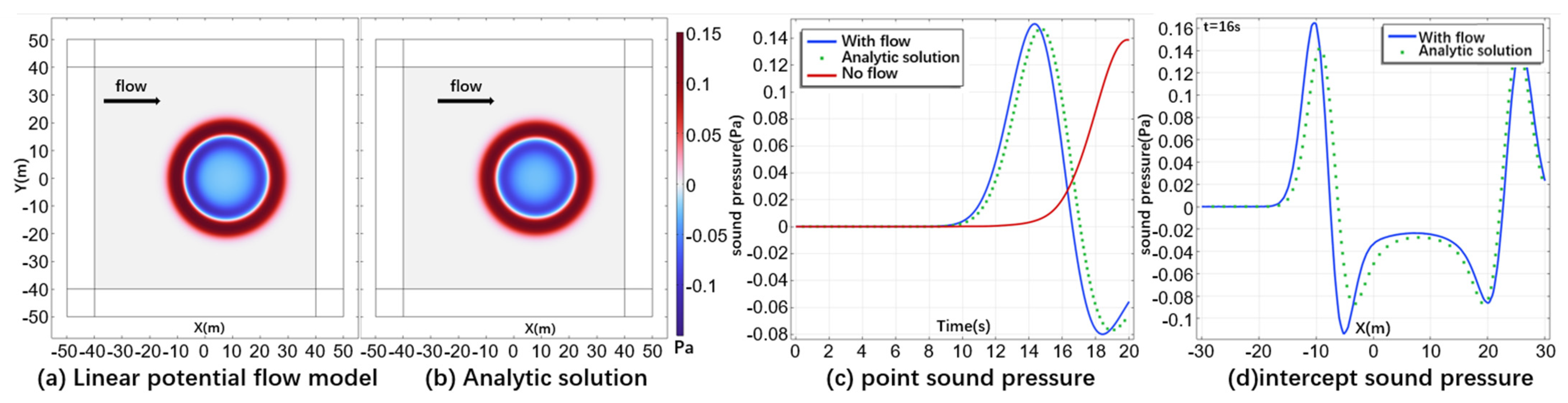
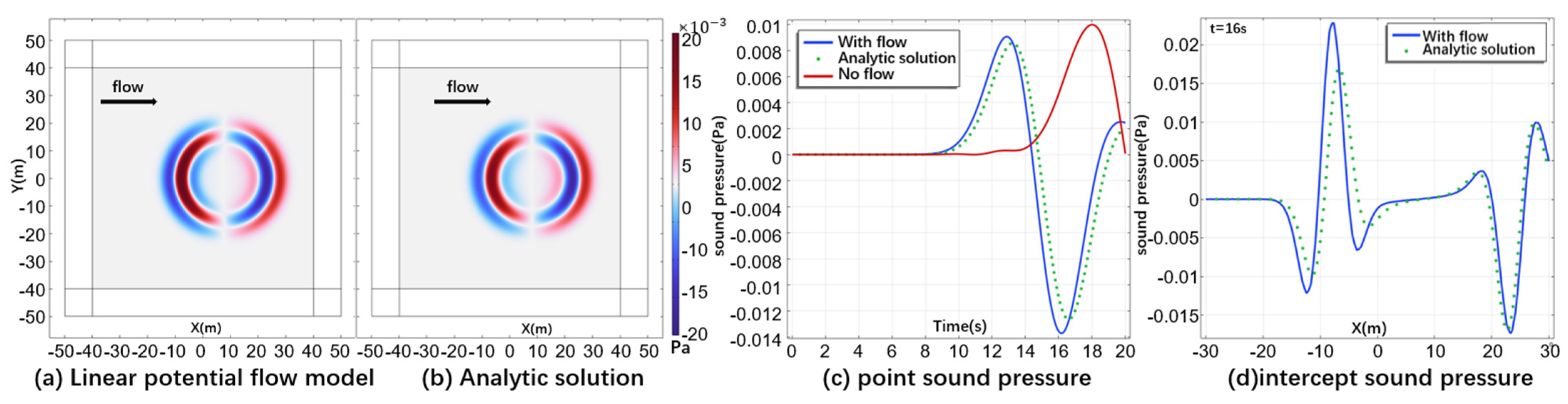
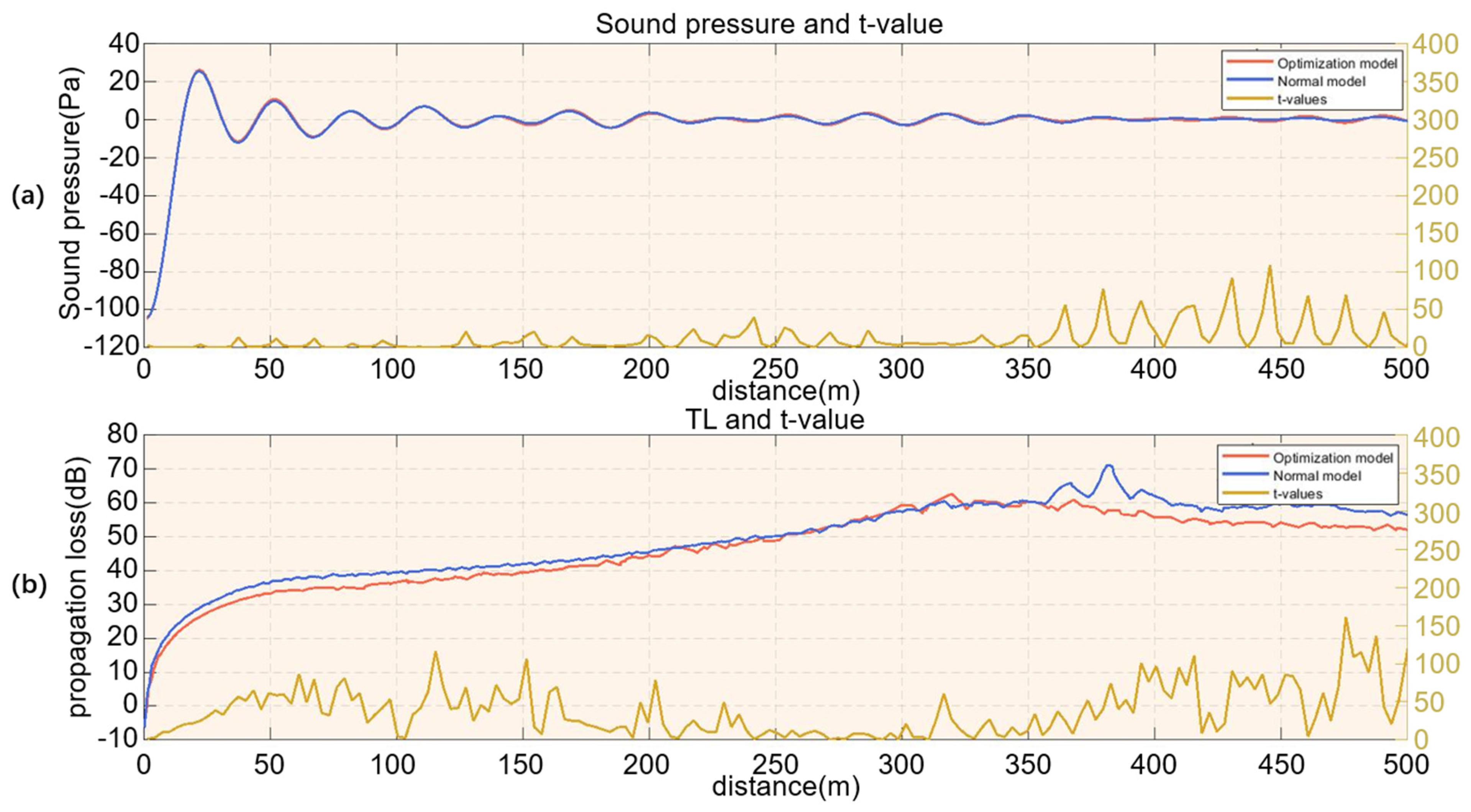
3.1. Model Accuracy Validation

In order to determine the accuracy of the model calculations, the analytical solution of the benchmark problem [42], the Gaussian pulse propagation case, is used in this paper to validate the sound field model. The reason for choosing a Gaussian pulse signal is, firstly, because a Gaussian pulse signal has short-time pulse characteristics, its reflection, and scattering phenomena will be more obvious, which helps to verify the accuracy of the finite element model. Secondly, because it takes a long time to calculate the analytical solution accurately, it is more favorable to choose a simple, ideal, and easy-to-generate Gaussian pulse signal to solve the problem. A Gaussian impulse propagation model is constructed from this benchmark problem and checked against the analytical solution. where the model is built in a dimensionless system, setting the ambient sound velocity to 1 and the density to 1.

The initial position of the Gaussian pulse is (0, 0) and the initial value sound pressure is $p_0$.

$$p_0=\exp [-\alpha (x^2+y^2\left)\right]$$

(17)

where $\alpha =\ln \left(2\right)/9$.

The x-direction background velocity of flow magnitude of the model is $u_x$, and the model is modeled by setting the $u_x$ of 0 and Ma, respectively. For $u_x$, which is equal to 0.5 in the flow-containing validation.

The expression for the parsing solution is as follows:

$$p\left(x,y\right)=\frac{1}{2\alpha }{\int }_0^{\mathrm{\infty }}\epsilon J_0\left(\epsilon r\right)\mathrm{e}\mathrm{x}\mathrm{p}(-\frac{{\epsilon }^2}{4\alpha })\left[\cos (\epsilon t-\frac{0.04}{2\alpha }\epsilon \sin \left(\epsilon t\right))\right]d\epsilon$$

(18)

where $J_0$ is a Bessel function of order 0, $r=\sqrt{{(x-Mat)}^2+y^2}$.

The results of the Gaussian impulse model against the analytical solution are shown in Figure 2. Figure 2a,b are the results of the linear potential flow and the analytical solution at $t=16$, respectively, and it can be seen that the acoustic wave deviates from the origin due to the influence of the flow. Figure 2c shows the sound pressure at coordinates (20, 10) for the linear potential flow and the analytical solution with respect to time, respectively, and Figure 2d shows the cutoff sound pressure at y = 0 at 16 s. The linear potential flow model and the analytical solution are in good agreement in both results.

To further validate the model, only the x-direction component of the original Gaussian beam is taken as the initial value for the experiment.

The experimental results are shown in Figure 3, and the model still exhibits good, accurate performance.

Expanding the 2D model to 3D, again placing a Gaussian pulse signal at position (0,0). At this point, the initial sound pressure $p_1$ can be expressed by the following equation:

$$p_1=\mathrm{e}\mathrm{x}\mathrm{p}[-\alpha (x^2+y^2+z^2\left)\right]$$

(19)

The corresponding background flow magnitude $u_x$ is unchanged. The analytic expression is lifted to three dimensions.

$$p_2\left(x,y,z\right)=\frac{1}{2\alpha }{\int }_0^{\mathrm{\infty }}\epsilon J_0(\epsilon r)\exp (-\frac{{\epsilon }^2}{4\alpha })\left[\cos (\epsilon t-\frac{0.04}{2\alpha }\epsilon \sin (\epsilon t))\right]d\epsilon$$

(20)

where $r=\sqrt{{(x-Mat)}^2+y^2+z^2}$. The experimental results obtained are shown in Figure 4.

Figure 4a,b show the results of the linear potential flow and the analytical solution at t = 16, respectively, where the sound field is also clearly affected by the flow in three dimensions. Meanwhile, Figure 4c represents the linear potential flow and the analytic solution of the acoustic pressure for the relevant time at the position of coordinates (10, 10, 10). Figure 4d shows the intercept sound pressure at 16 s for the two endpoints (−30, 10, 10) and (30, 10, 10), respectively. Both the 3D linear potential flow model and the analytical solution in the results are in good agreement.

3.2. Positive Application—Eddy-Influenced Sea Area Analysis

By increasing the computational speed of the model, it is possible to use the model to analyze the effects of flow in mesoscale phenomena and to take into account the effects of incoming flow on sound propagation in all directions in space.

The forward application of the model was selected in a portion of the Bering Sea region (171°E–179°E, 54°N–60°N). The identification of eddies was first carried out in the region using the no-threshold contour method, which showed that the mean amplitude of the eddies varied periodically throughout the year. The eddy influence region is constructed in a cold eddy centered at 177.7°E 54.5°N, and the non-acoustic sensitive regions of the model are optimized to varying degrees by using the sound-speed laminar junction spectral expression method to statistically account for changes in computational efficiency.

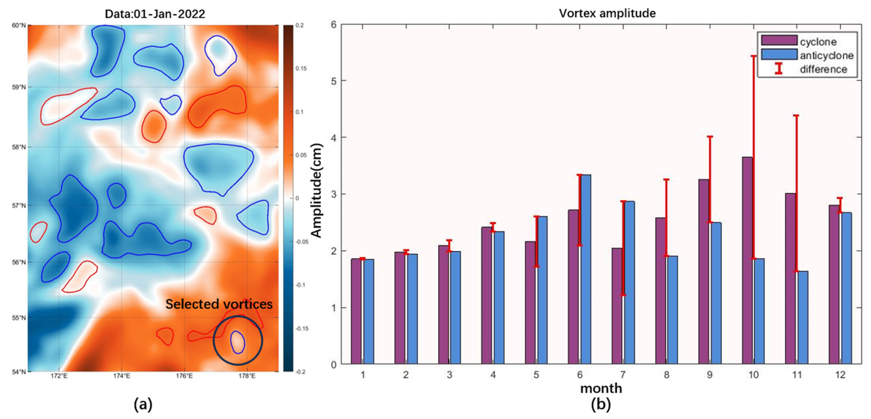
3.2.1. Identification of Eddies and Identification of Effects

Mesoscale eddies are generally defined as horizontally rotating bodies of water in the ocean with horizontal diameters of 10–500 km and durations ranging from a few days to a few years [43]. In the ocean, the flow direction of the flow field of mesoscale eddies tends to be parallel to the closed SSH or SLA contour, and by looking for the outermost closed curve, it is possible to determine the boundaries of eddies and thus achieve the purpose of identifying eddies. This has the advantage of avoiding the noise problem caused by calculating the flow field and is the most concise and direct way to identify mesoscale eddies. Since this paper does not involve the analysis of eddy complex results, the identification method fully satisfies the needs of the article study.

The SLAs and flow fields shown in Figure 5a are for April to July, where the anticyclonic eddy amplitude is stronger, and Figure 5b are for August to November, where the cyclonic eddy amplitude is stronger, which is briefly analyzed in the next section. Both SLA and sea surface flow fields serve as important identification criteria for mesoscale eddies and are, to some extent, compatible. Stronger flow fields are distributed near the region where the sea surface height anomaly is 0, i.e., near the sea level (the white region in the figure), and these regions are mostly recognized as eddy edges in the existing eddy identification methods.

The eddy identification flow of the no-threshold contour method utilized in this paper is shown in Figure 6:

The specific identification steps are as follows:

• The sea surface height anomaly data were imported into MATLAB2020b for preprocessing.
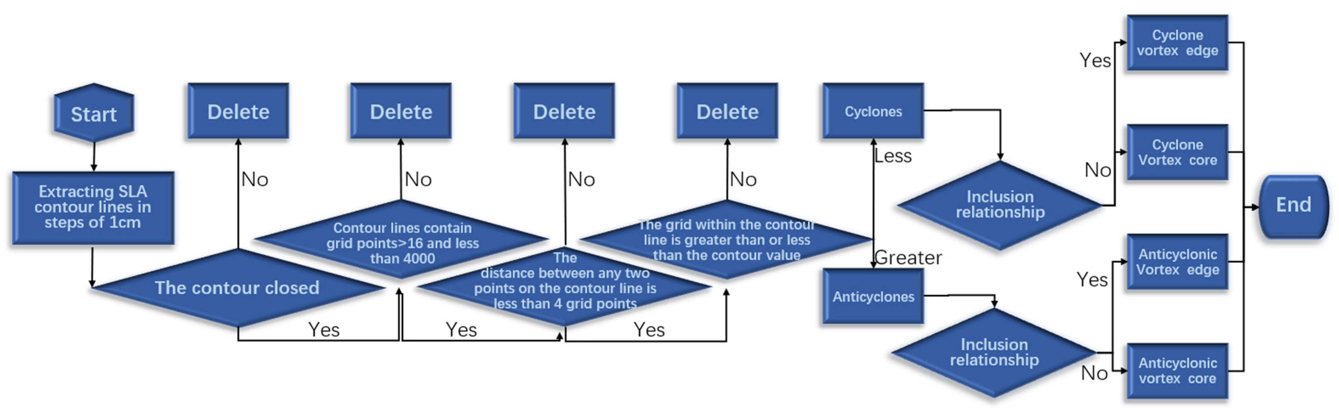
• All contours from −1 m to 1 m in the SLA data were extracted with a gradient of 1 cm, after which judgmental screening was performed for each contour.
• Determine if the contour is closed by determining if the contour is connected in the first place, and delete the contour if it is not closed.
• The number of all grid points contained in the contour is determined; if less than or equal to 16, it is considered that no vortex has formed and the contour is rejected; if greater than or equal to 4000, it is considered that the size of the mesoscale vortex is exceeded and that it may be a mixture of several vortices, and the contour is rejected.
• Determine whether the distance between any two points on the contour is less than 4 grid points; this step is to prevent the problem of recognizing vortices sticking to each other as well as recognizing the appearance of distortion.
• Judge whether the values of all the grid points in the contour line are greater or less than the data of the points on the contour line, eliminate the contour lines that do not meet the requirements, and classify the closed curves with the values of the grid points in the contour line less than the contour line as cyclonic vortex and the closed curves with the values of the grid points in the contour line greater than the contour line as an anticyclonic vortex. When the cycle of (2)–(6) steps is finished, two different sets of closed curves are returned.
• Determine the vortex kernel and vortex edge by the containment relationship between each group of closed curves, classify the curve that does not contain any other closed curve of the group as a vortex kernel, and classify the curve that does not have any other curves outside the curve that contain it as a vortex edge.
• All cycles end, returning the vortex edge of the cyclone, the vortex core of the cyclone, the vortex edge of the anticyclone, and the vortex core of the anticyclone.

Using the no-threshold contour method, monthly averages of eddy identification effects and eddy amplitudes for the Bering Sea region in 2022 are calculated in Figure 7.

Where the blue closed curve represents the cyclonic eddy (cold eddy) and the red closed curve represents the anticyclonic eddy (warm eddy). where the cyclonic eddy centers all contain anomalously large values of height in the region and the anticyclonic eddy centers all contain anomalously small values of height in the region. The sea surface heights and identified eddies in Figure 7a show that the identified eddies are basically distributed in the positive and negative intersection distributions of the sea surface height anomalies, which is also consistent with the region of fast flow in the flow field mentioned in the previous section.

In addition to this, the size and amplitude of the eddy are also important factors in determining the effectiveness of eddy identification. For the general definition of eddy amplitude as the difference between the height of the outermost sea surface of the eddy and the inner pole of the eddy, most of the general cyclonic eddies and anticyclonic eddies have an amplitude centered in the range of 2 cm to 4 cm. Monthly averages of the amplitudes of all cyclonic and anticyclonic eddies identified in each month of 2022 were made to obtain a monthly distribution of eddy amplitudes in the Bering Sea region, where most of the month eddies conform to the general eddy amplitude law, with a relatively weak mesoscale eddy in spring (January–March), a stronger cyclonic eddy in summer (May–July), and a stronger anticyclonic eddy in fall and winter (August–December). This is not contrary to the study of Zhabin et al., as they analyzed the seasonal distribution of eddies in the region in terms of the number of eddies.

The applicability of identifying vortices is analyzed in the following: As can be seen from the vortex identification in Figure 5a, the mesoscale vortices have clear contours and are in good agreement with the periphery of the SLA contours. For the purpose of this paper, the object of the study is the effect on acoustic propagation caused by stronger currents in mesoscale eddies. The distribution of currents in mesoscale eddies is often at the edges of the eddies, and it is also obvious from the superposition of the SLAs and the flow field in Figure 5 that the currents are stronger in the region where the height anomaly is 0. This also confirms the accuracy of this vortex identification method for vortex edge identification. Based on the effective identification of the edges of the vortex, one vortex that is more independent, less disturbed by other vortices, and with a vortex size that puts low computational pressure on the model construction is selected for study.

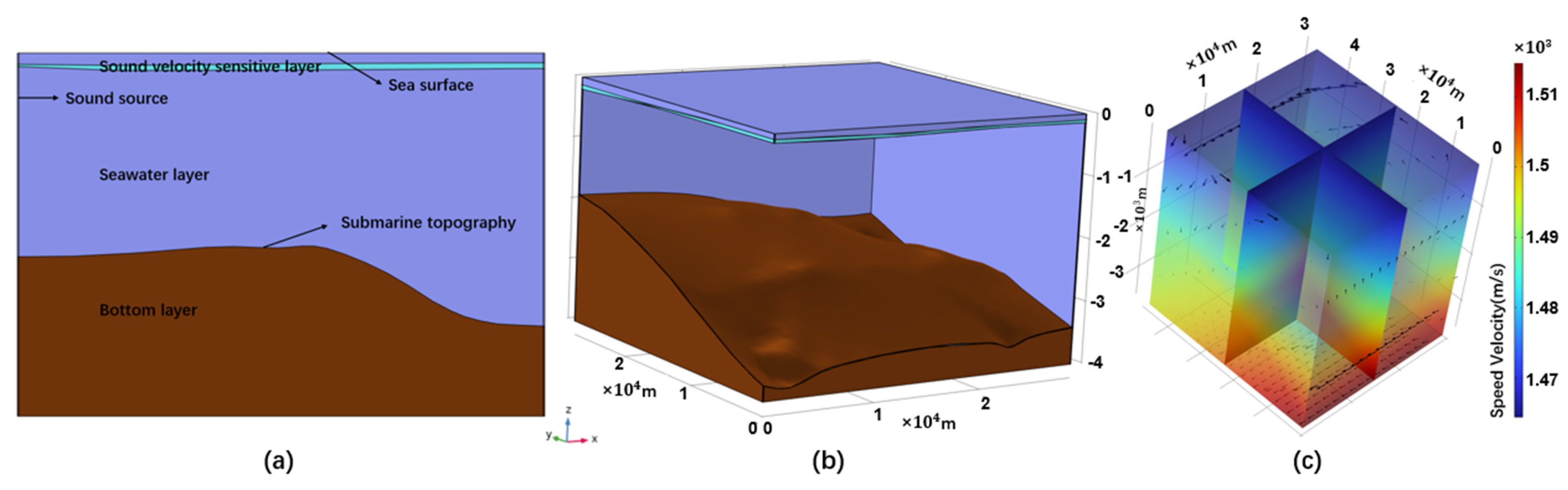
3.2.2. Construction of the Eddy Model

The scale of the modeling is determined based on the range of the identified eddies. Before building the model, the data such as sound velocity, flow velocity, and topography are computed and reconstructed, and the latitude and longitude of the data are fitted to the three-dimensional data with the width and depth of the length.

The speed of sound is calculated using the Mackenzie empirical formula for the nine-speed of sound calculations, the formula is recommended by UNESCO which is given below:

$$\begin{array}{c}C=1448.96+4.591T\times {10}^{-2}{T}^2+2.374\times {10}^{-4}{T}^3+1.340\left(S-35\right)\\ +1.630\times {10}^{-2}D+1.675\times {10}^{-7}{D}^2-1.025\times {10}^{-2}T\left(S-35\right)\\ -7.139\times {10}^{-13}T{D}^3\end{array}$$

(21)

where C denotes the calculated speed of sound in m/s, T denotes the temperature in °C, S is the salinity in parts per thousand, and D denotes the depth in m.

In data reconstruction, the data matrix of the two-point interrupted surface is first calculated, and the variable $J$ is defined as the number of interpolation points, so that the longitude interval between two neighboring interpolation points is ${(x}_2-x_1)/J$, the latitude interval is ${(y}_2-y_1)/J$, The latitude and longitude of the nth data point in the latitude and longitude interpolated data string is $x_1+J\times (n-1)$, so that the one-dimensional coordinate data string of the section is obtained.

Normalize the cross-section latitude and longitude according to the following formula for converting latitude and longitude to distance:

$$D=R\times {\cos }^{-1}(\cos y_1\times \cos y_2\times \cos \left(x_1-x_2\right)+\sin y_1\times \sin y_2)$$

(22)

where the mean radius of the Earth is defined as R = 6,371,000 m, D is the calculated distance between the two points, $x_1$ and $x_2$ are $\frac{lon\times \pi }{180}$ of the start and end points, $y_1$ and $y_2$ are $\frac{lat\times \pi }{180}$ of the start and end points.

Then the normalized distance of the nth data point is $J\times (n-1)\times D/(J-1)$.

Based on the planning equations listed above, the data matrix is planned layer by layer using the sea level at the southwest corner of the matrix, where the vortex is located, as the coordinate origin, and Figure 8a shows one layer of the three-dimensional data structure. After that, the 3D data matrix of sound velocity, northward flow velocity, and eastward flow velocity can be obtained, as shown in Figure 8c. Since the seafloor topographic data are only available in latitude and longitude positions and corresponding depths, they are planned as a two-dimensional data matrix, and in Figure 8b, you can see that the two-dimensional topographic data is filled to form a three-dimensional topographic layer.

After the base data, the geometric model also needs to be constructed, where the geometric boundaries are W × D × H, W is the length of the watershed, D is the width of the watershed, and H is the depth of the water.

The model is surrounded by a Perfectly Matched Layer (PML) with a thickness of 75 m in addition to the upper and lower surfaces, which are used to solve the problem of calculating the sound field in an infinite sea area in a finite space.

In the model setup, the parameters of the propagation loss to be studied are defined, allowing the model to calculate the propagation loss in each region within the sound field. The propagation loss expression is given below.

$$TL=-10{\log }_{10}\frac{I_r}{I_0}=-20{\log }_{10}\frac{p_r}{p_0}$$

(23)

In this equation, $I_0$ is the sound intensity at a distance of 1 m from the source, and $I_r$ is the sound intensity at various locations in the sound field, and the logarithm of the ratio of the two is taken as the value of the propagation loss. The sound intensity $I$ can also be expressed as $p^2/{\rho }_0{c}_0$.

In the seafloor terrain part, in order to simulate the effect of the seafloor sediment on the absorption of acoustic energy and seafloor scattering, the seafloor terrain is set in two layers. One layer is the impedance layer, which reflects the reduction of acoustic energy by the sediment, and here it also affects the scattering intensity of the seafloor. The other layer is the hard sound field boundary, which embodies a change in the direction of the sound waves. The superposition of two substrate layers allows for the characterization of the absorption and scattering of a single substrate during the process of moving from a soft sound field boundary to a hard sound field boundary. The specific transfer impedance Z is defined by the following equation.

$$Z=\rho \ast c$$

(24)

where $\rho$ is the material density, $c$ is the speed of sound propagation in the material.

The 2D plane is intercepted in the 3D sound field as a schematic representation of the sound field distribution, as shown in Figure 8a, and the free quadrilateral mesh is distributed in all the computational domains, including seawater, terrain, perfectly matched layer, and sound source.

3.2.3. Extraction of Sensitive Areas

In the finite element sound field calculation process, in order to ensure the accuracy of the calculation results and prevent distortion of the calculation results, the maximum size of the general grid is set to 1/5 wavelength. However, in practical application, we found that optimizing the mesh of some sound field regions and increasing the mesh size appropriately have less effect on the overall propagation law of the sound field. As shown in Figure 9, in constructing the two-dimensional sound field, one of the models (Figure 9a) was modeled and computed in the seawater layer using a normal grid of 1/5 wavelength, the other model (Figure 9b) was computed with a normal grid of 1/5 wavelength in the sound source section, sea surface and seafloor section, and an optimized grid of 1/3 wavelength for the rest of the section. The resulting calculations for the two models do not change much except in resolution. So, the team managed to find a better optimization scheme to reduce the number of meshes as much as possible while ensuring computational accuracy, in order to achieve the effect of increasing the computational speed and realizing the 3D sound field computation.

In the region where the gradient of sound velocity change is large, as well as the location of the sound source, small changes have a great impact on the calculation of the sound field over long distances, which should still be divided into denser grids to ensure the accuracy of the calculation results. The whole idea of all the optimization of the grid is based on the degree of change in the speed of sound. The region where the acoustic velocity gradient changes sharply is generally the sound velocity thermocline, but the degree of sharp change for the stratification and the division range of the stratification is an uncertain quantity, so this paper adopts the acoustic velocity layer junction spectral expression to determine the range of the sound velocity thermocline and then re-distribute the mesh structure for the different regions of the acoustic field.

The endpoints of the spectral peaks are determined by detecting the top and bottom roots of the spectral peaks at the most valuable points according to the method of the most value of the curvature region of the endpoints of the peaks of the stratification.

The curvature of the sound velocity thermocline spectrum can be defined by differentiation, indicating the degree of bending of the curve away from a straight line, and is obtained according to the following equation:

$$K=\frac{x^{″}}{\sqrt{{(1+x^{\prime 2})}^3}}$$

(25)

where K is the curvature, $x^{\prime }$ is the first-order derivative of the speed of sound with respect to depth, and $x^{″}$ is the second-order derivative of the speed of sound with respect to depth.

The identification of the endpoints of the peaks of the leapfrog spectrum is, in fact, the identification of the extreme values of the curvature of the speed of sound. The curve in Figure 10c is the sound velocity curvature obtained after Equation (25), and the two points E and F are obtained by taking the extreme value of the curve, and the region between the two points indicates the region where the sound speed changes to a greater extent. Correspond the depths where E and F are located to the sound velocity profile curves as well as the sound velocity gradient curves. As shown in Figure 10a,b, the region between the two points of the acoustic leapfrog layer exhibits a clear gradient characteristic of the sound velocity thermocline. The two dividing lines can be used as a dividing line between the water bodies above and below the thermocline and, at the same time, as a dividing line between sound velocity-sensitive areas and other water bodies. The same process is done for the 3D sound velocity field to extract the upper and lower sub-interfaces of the water body in the sound velocity-sensitive area, and the mesh is optimized for the non-sensitive areas therein to improve the overall computational speed of the model.

3.3. Reverse Application—Sound Velocity Inversion in Current-Affected Waters

Convection-influenced waters for sound velocity inversion are an extension of modeling applications in the field of acoustic inversion, and the main focus is on the effects caused by ocean currents on acoustic propagation. The calculation of the standard model in the paper yields a sound velocity inversion optimization formula, which can be used to optimize a sound velocity inversion calculation method affected by flow velocity, such as a sound velocity inversion method based on the number of counting wavelengths in the domain. In this paper, data from the Shallow Water Experiment (SW06), conducted in 2006 near the New Jersey Continental Shelf in the United States, were selected to complete this part of the application. The experiment was conducted by multiple institutions in multiple countries. A number of scholars have already utilized this experimental data for acoustic analysis [35,36,44]. So, the use of SW06, which is the current-laden experimental data with a high level of confidence and verified by many scholars. The data used in this paper is partly WHOI data deployed on 34 moorings in a long and across shelf.

3.3.1. SW06 Measured Data

There are two types of environmental moorings for the SW06: the less heavily instrumented Structure Moorings and the heavily instrumented Environmental Moorings. This paper uses experimental data from heavily instrumented Environmental Moorings; the coordinate positions are shown in Figure 11. In contrast to the light units, the heavy units are fitted with several temperature and pressure sensors, as well as conductivity (salinity) sensors and current profilers (ADCP). This allows the heavy-duty mooring system to measure a wider variety of environmental data, which is more conducive to the analysis of model calculations.

The time of the experiment was chosen to be 30 August 2006, and the hourly data from Environmental Moorings were averaged to obtain a profile data set for each point on that day, with the sensor depths and measured flow velocities for the moorings shown in Figure 12. The direction of flow is positive to the east in the direction of the parallel meridian.

3.3.2. Sound Velocity Inversion Model Design

In order to further investigate the effect of the flow in the eddy on the sound field calculation and to prove the validity of the optimized model, a number of standard models are set up to simulate different depth regions in the ocean with different sound velocities and to simulate the strength of the eddy or tidal currents with different flow velocities in order to build a local model. The simulation results characterize the effect of the velocity of flow term on acoustic tomography through the perspective of the acoustic pressure inversion velocity of flow in acoustic chromatography. At the same time, the velocity of flow in the standard model was increased appropriately to ensure that the velocity of flow influence term on the inversion was large enough to reduce the impact of the remaining errors on the inversion.

A perfect matching layer is set at all the boundaries of the model to prevent the influence of boundary reflections on the sound field calculation. The source frequencies of the model were set to 50 Hz and 100 Hz for two separate calculations. Horizontal probes are placed at the depth of the sound source in each model, and parameters such as sound pressure and propagation loss of the source intercept are derived for subsequent analysis and processing after model calculation.

By modeling the models separately for different flow velocities and at different sound velocities, the computational results of the 63 models used to compute the flow velocity influence term were obtained, and some of the models for various sound velocity ranges are illustrated in Figure 13. There is not much difference between the different models in terms of 3D calculation results, and the exported data needs to be processed for further analysis.

3.3.3. Fitting Improved Equations

A solution based on the number of counted wavelengths in the domain was used for the calculation of the sound velocity during the inversion process [28]. The sound pressure data of the model cutoff line was analyzed by Prony’s method to obtain the phase information of the sound waves, and the total number of wavelengths between the two endpoints of the cutoff line was obtained by counting the same phases. At this point, the standard model inverse sound velocity can be derived from the following equation:

$$c_e=\frac{D{f}_0}{N_{\lambda }}$$

(26)

where D is the length of the two endpoints of the intercept line, $N_{\lambda }$ is the total number of statistical wavelengths, and $f_0$ is the current acoustic frequency.

The sound pressure intercept data for all modeled sound source locations constructed were exported and inverted to obtain the calculated sound velocity under the influence of flow for different background flow and sound velocity conditions.

The curves of sound velocity values for different flow influences obtained from the model inversion are shown below (Figure 14).

It can be seen that when the seawater sound velocity v is different, the sound velocity obtained by inversion, given a uniformly varying flow velocity, is not simply a linear summation of the seawater sound velocity v and the flow-influenced sound velocity. When the flow velocity is 0, the sound velocity obtained from the inversion varies for different sound velocity v conditions, so the model with a linearly varying sound velocity v and a flow velocity of 0 is again set for the sound velocity inversion.

The inverted sound velocity that will be calculated actually incorporates the effects of the flow. When we split the actual sound velocity into two parts, i.e., the current seawater sound velocity and the flow-influenced sound velocity, we get the following:

$$c_e=v+\gamma u+\beta$$

(27)

where $c_e$ is the initial sound velocity obtained from the inversion, $v$ is the current seawater sound velocity, $\gamma$ is the flow influence coefficient, and $\beta$ is the remaining influence.

After subtracting the seawater sound velocity when the velocity of flow $u$ is 0, the remaining term can be regarded as a linear function with the velocity of flow $u$ as the independent variable, which can be solved by linear fitting as shown in Figure 15a.

An RMSE of 1.39 was obtained for the fitted straight line and flow influence terms, and the value of the flow influence coefficient $\gamma$ = 1.117.

Since the difference between the sound velocity obtained by inversion and the actual sound velocity is not equal to or close to 0 when the flow velocity is 0, Figure 15b shows the process of the inversion sound velocity value when the actual sound velocity is different in magnitude. That is, the inversion sound velocity minus the actual sound velocity is not a straight line with a slope of 0. The size of this straight line varies under different actual sound velocity conditions, so the remaining effect $\beta$ is also related to the seawater sound velocity. Since the seawater sound velocity term $v$ is not directly available, the inversion-measured sound velocity is used as an approximate substitute to re-model the different seawater sound velocities in the absence of flow.

The obtained inverse sound velocities $c_e\left(i\right)$ were first subtracted from the respective seawater sound velocities $v\left(i\right)$, to obtain the residual equations, which were fitted.

The graphs of the simple fits are shown in Figure 15c,d, and the expression for the residual term is obtained as ${\beta }_1=\sigma {\left(v\right)}^{\tau }$, the fit yields $\sigma$ = $2.236\times {10}^{-10}$, $\tau$ = 3.456. This fitting method yielded an RMSE of 7.793. Since the speed of sound therein cannot be obtained directly from the inversion, $v$ is approximated by replacing it with the inverted speed of sound, $c_e-\gamma u$, which is subtracted from the flow term.

A simple fit yields the following expression for the inverse sound velocity correction.

$$v_{e1}=c_e-\gamma u-\sigma {(c_e-\gamma u)}^{\tau }$$

(28)

Figure 15e,f represent Gaussian fitted curves, and the residual expressions obtained after fitting are as follows.

$${\beta }_2=a_1{e}^{-{\left((v-b_1)/c_1\right)}^2}+a_2{e}^{-{\left((v-b_2)/c_2\right)}^2}+a_3{e}^{-{\left((v-b_3)/c_3\right)}^2}$$

(29)

This fitting method yields an RMSE of 1.95, which is a better fit than the simple fit. The corrected expression for the inverted sound velocity for the Gaussian fit was similarly obtained by replacing the actual sound velocity with $c_e-\gamma u$.

$$v_{e2}=c_e-\gamma u-a_1{e}^{-{\left((c_e-\gamma u-b_1)/c_1\right)}^2}-a_2{e}^{-{\left((c_e-\gamma u-b_2)/c_2\right)}^2}-a_3{e}^{-{\left((c_e-\gamma u-b_3)/c_3\right)}^2}$$

(30)

Here, $a_1=54.78$, $b_1=1983$, $c_1=66.98$, $a_2=25.38$, $b_2=1886$, $c_2=59.21$, $a_3=31.31$, $b_3=1735$, $c_3=244.6$.

The residual correction obtained using a Gaussian fit begins to decay at actual sound velocities above 2000 m/s, and it applies from 0 to 2000 m/s. In reality, sound velocities this fast do not occur in seawater.

4. Discussion

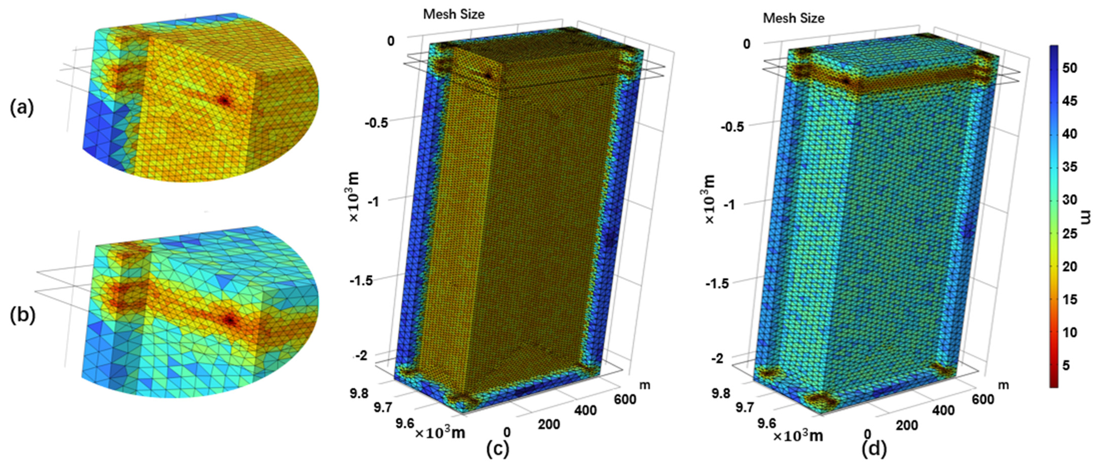
4.1. Grid Differentiation Model Calculation Results

The density of the grid structure of the finite element model greatly affects the computational speed of the model, and the grid size of different regions is optimized according to the results of the sound velocity classification so that the overall number of grids in the model is reduced in order to improve the computational speed.

Based on the results of the sensitive area classification in the previous section, different degrees of optimized and unoptimized models were constructed to simulate the sound field in the intra-eddy region. As shown in Figure 16c,d, showing the schematic of the different models without mesh optimization and after mesh optimization, Figure 16a,b are zoomed-in views of the sound-speed-sensitive region.

The server configuration information used for the model calculations is shown below:

• Operating system: Window 10 (20H2)
• CPU: AMD EPYC 7402 24-Vore Processor 2.80 GHz *2 (AMD, Made in America)
• RAM: 512 GB (SK Hynix, Made in Korea)

After the calculation, the number of meshes and computation time are counted to get a comparative list of model performance before and after optimization (

Table 1. Model calculation efficiency table.

Model Type	Maximum Grid Size for Sensitive Layers	Maximum Grid Size for Optimization Layer	Grid Construction Time	Computation Time
Traditional Model	λ/5	λ/5	128 s	6 h 24 min 16 s
Optimization Models1	λ/5	λ/4	72 s	29 min 27 s
Optimization Models2	λ/5	λ/3	36 s	10 min 7 s
Optimization Models3	λ/5	λ/2	17 s	3 min 9 s
Optimization Models	λ/5	λ	11 s	1 min 26 s

). wherein the model with the changed number of optimization layer grids is treated as an optimization model and the unchanged model is treated as a traditional model.

In terms of computation time, as the maximum grid size of the optimization layer decreases, a significant increase in grid construction time occurs, while the model computation time increases exponentially. Fewer meshes also mean that the computations take up less memory, allowing a wider spatial sound field to be analyzed under the same conditions.

In order to find the optimal grid size setting for the optimization layer, we take the average propagation loss error accuracy of 3 dB as the limit and compare it with the standard model to gradually approximate the critical grid size of the grid optimization model. By calculation, the criticality is reached when the grid size of the optimized grid layer is set to λ/1.852, at which time the grid construction time is 15 s and the model calculation time is 2 min 47 s. The optimization saves 98% of the computation time of the model calculation. By optimizing the model mesh, the computable range and computation speed of the 3D model can be greatly improved.

In order to test the stability of the optimized grid density, the model is constructed based on the baseline position translation for calculation, and the calculation results are shown in the following table (

Table 2. Translational modeling and its computational time.

X-Direction Translation (m)	Y-Direction Translation (m)	Model Computation Time	X-Direction Translation (m)	Y-Direction Translation (m)	Model Computation Time
5000	0	3 min 6 s	0	5000	3 min 10 s
4000	0	3 min 10 s	0	4000	3 min 2 s
3000	0	3 min 7 s	0	3000	3 min 0 s
2000	0	3 min 5 s	0	2000	2 min 53 s
1000	0	2 min 52 s	0	1000	2 min 45 s
−1000	0	3 min 10 s	0	−1000	3 min 6 s
−2000	0	3 min 4 s	0	−2000	3 min 4 s
−3000	0	2 min 52 s	0	−3000	2 min 50 s
−4000	0	2 min 53 s	0	−4000	3 min 6 s
−5000	0	3 min 5 s	0	−5000	3 min 4 s

).

Using the optimal grid size to pan 5 times in different directions along x and y, respectively, 20 calculations were obtained, and the computation times obtained were all below 3 min 10 s, the increase in computing speed was 98% or more, and the above average calculation time is 3 min 3 s, to prove the feasibility of the optimization of the grid. Subsequent experiments will be performed based on the best-optimized grid density.

In order to compare the differences between the calculation results of the two models, the intercepts at the same locations of the two models were intercepted, the sound pressure and propagation loss at the intercepts were calculated, and the t-test was applied to the values of the sound pressure and propagation loss intercepts of the eddy intercepts. It is dealt with as follows: (1) divide the two sets of data equally every 2 m; (2) calculate the t-value of the two sets of data using the t-test formula; (3) calculate the degrees of freedom of each set of data; (4) summarize the t-value of each set of data. The t-test formula is as follows:

$$t=\left({\stackrel{̿}{x}}_1-{\overline{x}}_2\right)/\sqrt{s^2/n_1+s^2/n_2}$$

(31)

where ${\stackrel{̿}{x}}_1$ and ${\overline{x}}_2$ are the means of the two sets of data, s is the pooled standard deviation of the two sets of data, and $n_1$, $n_2$ denote the sample size of the two sets of data, respectively. The expression for the pooled standard deviation s is given below:

$$s_p^2=({(n}_1-1)s_1^2)+((n_2-1)s_2^2)/n_1+n_2-2$$

(32)

In the formula, $n_1$ denotes the size of the first set of samples, $n_2$ denotes the size of the second set of sample capacity, and $s_1$, $s_2$ denote the standard deviation of the two sets of samples, respectively.

When the significance level is set to 0.05, the sound pressure curve, the propagation loss curve, and the t-value curve of the data intercepts are obtained, as shown in Figure 17. Figure 17a is the sound pressure and t-test absolute magnitude for both models, and Figure 17b is the propagation loss and t-test absolute magnitude for both models.

Most of the significant locations of the differences in the sound pressure intercepts are at the peak and trough locations; the overall acoustic phase conformity is high; and the differences between the two models gradually increase as the propagation distance increases. In the model propagation loss comparison, it can be obtained that the propagation loss of the optimized model is slightly smaller than that of the normal model, and after averaging, the average TL of the optimized model is obtained to be 47.46 dB and that of the normal model is 50.81 dB. During the propagation of acoustic energy through more grids, the rate of decay is always greater than in the less-grid condition, and the main differences for the data are similarly clustered at the peak points.

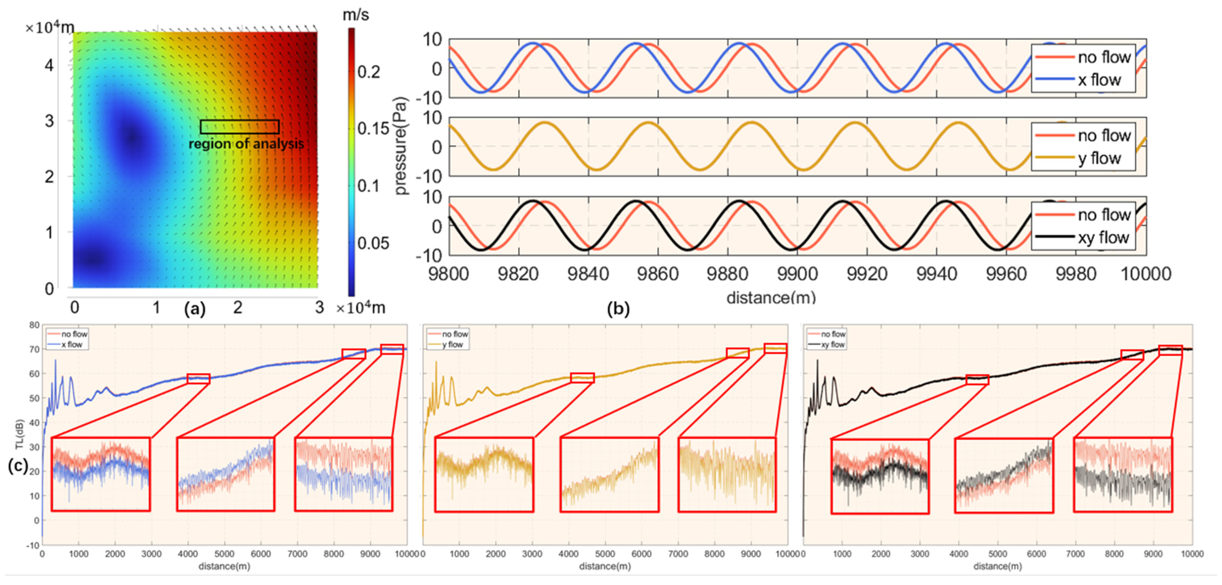
4.2. Results of Mesoscale Eddy Sea Sound Field Analysis

Application of the model to the analysis of selected cold eddies in the Bering Sea region to analyze the effect of flow on the propagation of the acoustic field at the eddy edges, where the effect of flow influence is stronger, the 3D model construction area is as boxed in Figure 18a. The sound field is computed sequentially for the no-flow case, the sound field when x-direction flow is added, the sound field when y-direction flow is added, and the sound field when xy-direction flow is added at the same time, and the sound pressure and propagation loss of each sound field are derived and analyzed.

Figure 18b shows a comparison of sound pressure against sound field cutoffs. It can be calculated that if there is only the influence of the flow along the sound field propagation direction, the sound field propagation will deviate from the original sound field, and the degree of deviation can reach about 3.5 m in the range of 10 km, while the flow in the perpendicular direction of sound propagation has no deviation effect on the sound field.

Figure 18c shows a comparison of sound propagation losses for sound field intercepts. The flow along the direction of propagation of the sound field increases the error in the calculation of the sound propagation loss, and this error can be up to 1 dB after a propagation range of 4 km. The flow field in the perpendicular sound field propagation direction increases the sound propagation loss throughout the process, but the effect of this increase is much less than 0.1 dB negligible.

It is worth noting that when modeling in the direction of vertical eddy flow, the flow along the direction of sound propagation itself is much smaller than the flow in the direction of perpendicular sound propagation, so the effect of the flow along the direction of sound propagation should be much larger than that of the flow in the direction of perpendicular sound propagation. That is, the eddy will have a greater effect on sound propagation in the direction of its flow.

4.3. Inverse Optimization Analysis Results

In which the sound field is modeled in each Mooring’s area, each model is 200 m wide and 500 m long, with the depth controlled by the terrain. The background data used in the model were derived from satellite remote sensing reanalysis data from Copernicus. A 50 Hz sound source was first used to emit and calculate the sound pressure intercept in the longitude direction at the corresponding depth of each transducer in each region, and the inverse sound velocity at that depth was obtained using the sound pressure intercept calculation. The optimized sound velocity is obtained by substituting the inverse sound velocity into the optimization formula, and then compared with the measured data, the fitting results obtained from the optimization Formula (1) are shown in Figure 19.

A set of inversion results can also be obtained from Equation (2), measured with four moorings at different frequencies as follows (Figure 20):

The RMS calculated in

Table 3. RMS values between different sound velocity curves under a 50 Hz sound source.

50 [Hz]	Moor29	Moor30	Moor32	Moor33	Mean Value
Inverse Speed of Sound RMS	15.133	15.003	14.953	23.593	17.170
Improved Speed of Sound1 RMS	25.979	11.170	9.187	8.324	13.665
Improved Speed of Sound2 RMS	20.302	7.039	5.144	11.739	11.056

and

Table 4. RMS values between different sound velocity curves under a 100 Hz sound source.

100 [Hz]	Moor29	Moor30	Moor32	Moor33	Mean Value
Inverse Speed of Sound RMS	12.116	14.649	14.335	23.912	16.253
Improved Speed of Sound1 RMS	23.167	10.318	9.332	10.228	13.261
Improved Speed of Sound2 RMS	17.236	5.862	4.477	12.702	10.069

Means values are averaged using raw data.

are the RMS of the difference between the inversion data and the measured data at different source frequencies, respectively, and what is indicated is the degree of difference between the inversion data and the measured data. From the comparison of the mean RMS values at 50 Hz and 100 Hz, the higher frequency inversion results in smaller calculated RMS compared to the lower frequencies, indicating that the results are closer to the measured values, regardless of whether or not the speed of sound inversion optimization formula is used. The RMS means of the inversion optimization formulas in Table 3 and Table 4 are reduced compared to the RMS means of the direct inversion, and the inversion Formula (2) reduces the RMS more than the inversion Formula (1). This not only shows that the improved formula can eliminate the errors brought by the flow rate and the rest of the terms in the partial sound pressure inversion of the sound velocity and achieve the effect of optimizing the inversion results but it also can be concluded that the Gaussian fitting is better than the simple fitting.

5. Conclusions

In this paper, based on satellite remote sensing data, a three-dimensional finite element fast acoustic field model under the influence of currents is proposed for rapid computation of ocean-acoustic remote sensing in mesoscale eddy or current seas. The innovations in this paper are shown below.

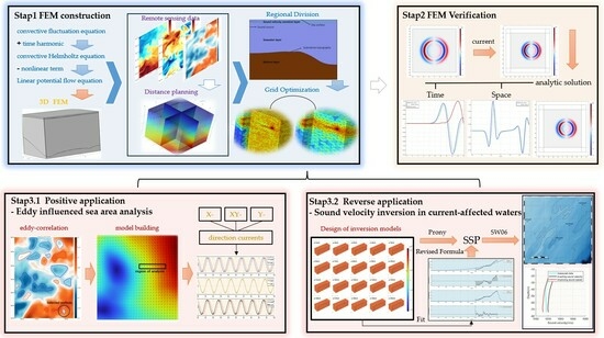
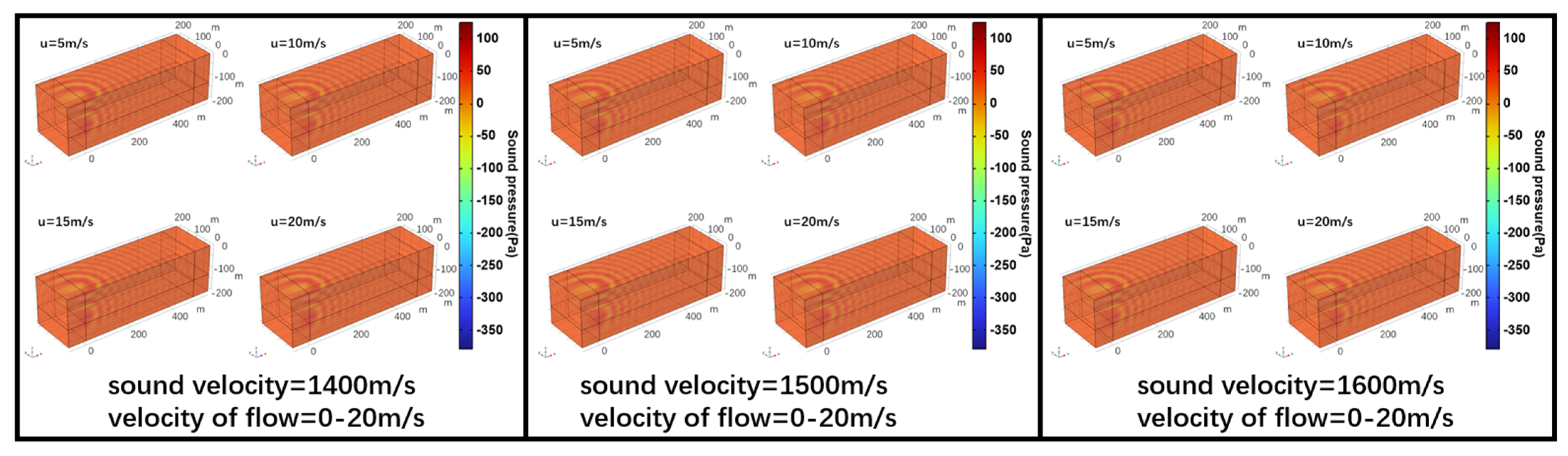
• Based on the linear potential flow theory, a three-dimensional finite element acoustic field model with the ability to analyze the acoustic field under the influence of flow is constructed, which can be used to analyze the acoustic field in the region with a large degree of influence of flow, such as mesoscale eddies and tidal currents. In this paper, after eddy identification, the acoustic field within a mesoscale eddy in the Bering Sea is modeled, and acoustic field parameters such as sound pressure and propagation loss of the acoustic field are calculated.
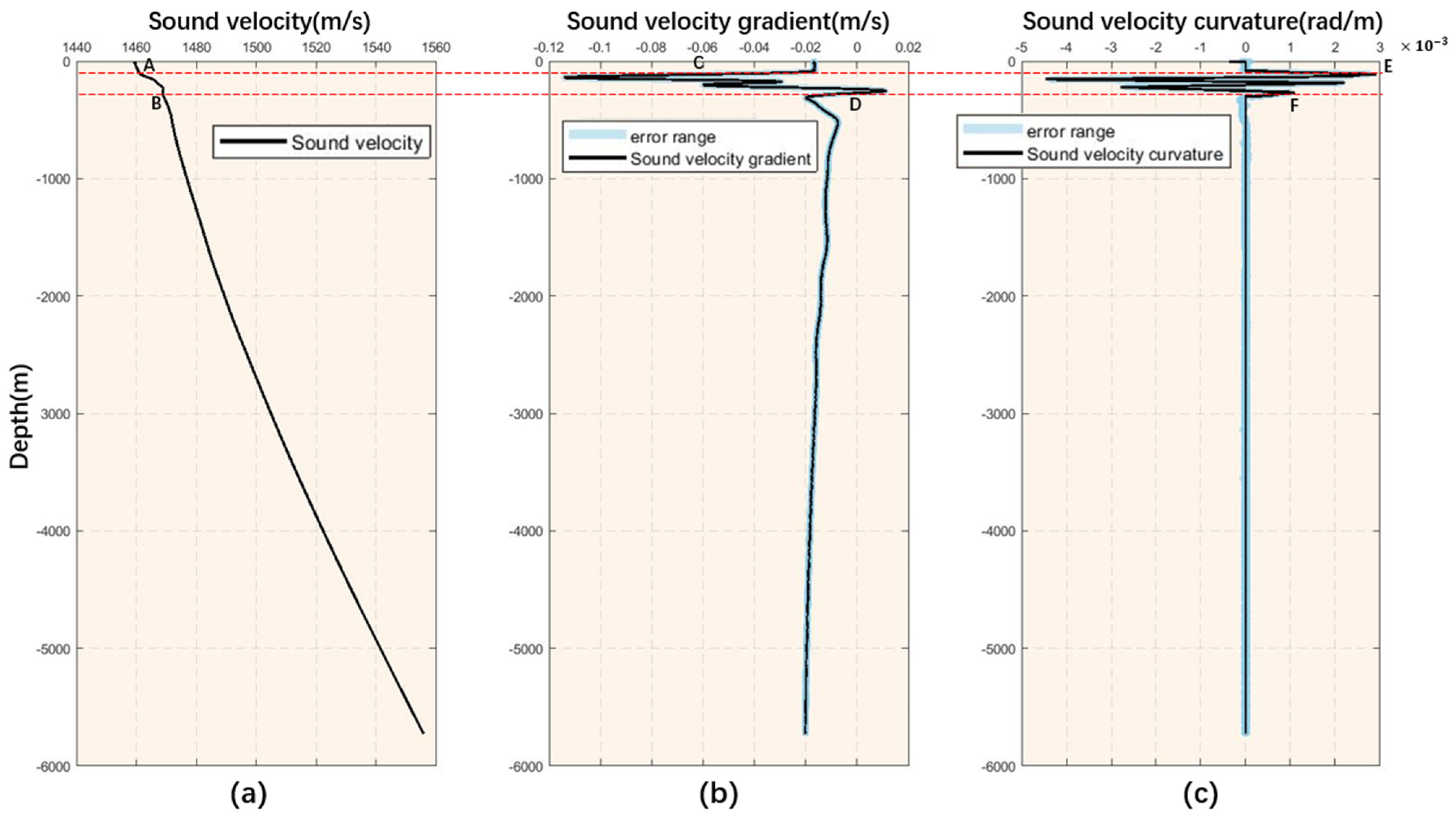
• The mesh structure of the finite element model is optimized to form the sound velocity laminar junction spectral expression by detecting the optimum point of the upper and lower roots of the spectral peaks of the sound velocity profile, thus determining the endpoints of the spectral peaks. According to this method, the sound velocity-sensitive layer and optimization layer are divided, and different grid densities are divided for different regions, so as to improve the computational speed of the model and form a fast field model. After gradually approximating the optimal grid size, the optimum is reached when the grid size of the optimization layer is set to λ/1.852, which saves about 98% of the computation time compared with λ/5, and the computation results maintain a small error.
• Applying the model forward to analyze the Bering Sea region, it is found that eddies have a greater effect on the propagation of the sound field along their flow direction, and the effect on the sound field offset can be up to 3.5 m and the effect on the propagation loss error can be up to 1 dB at a range of 10 km.
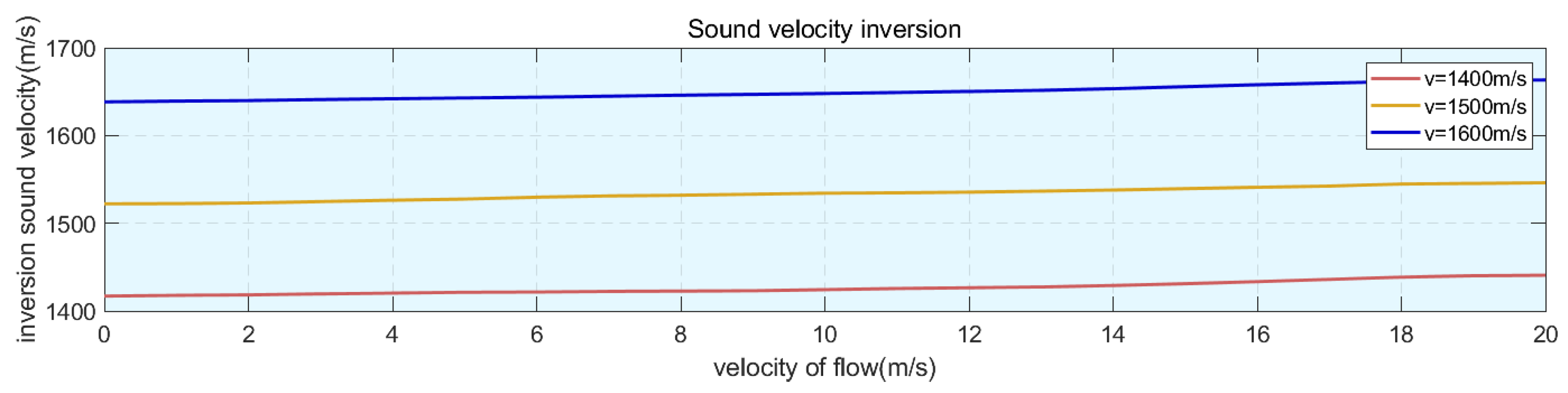
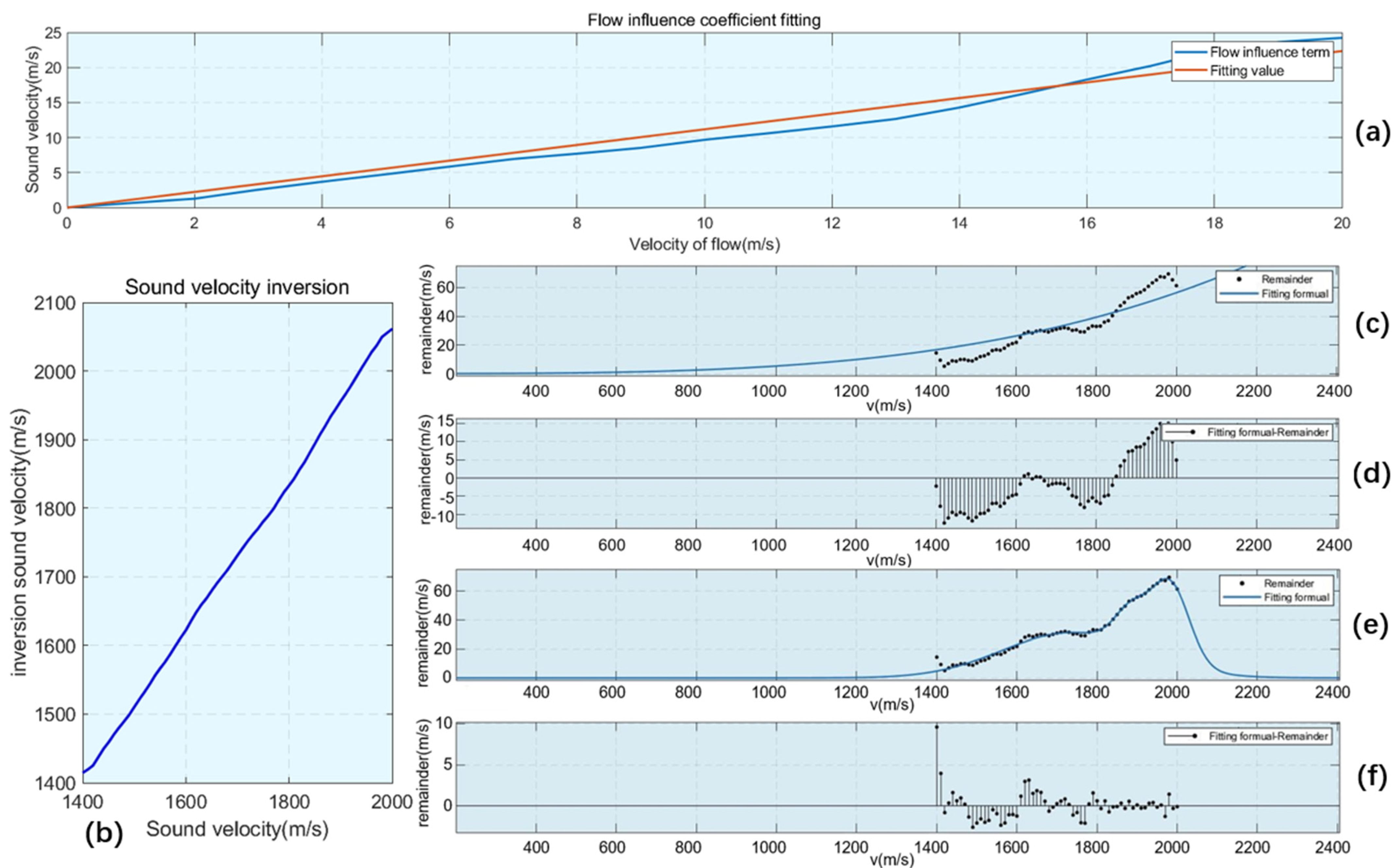
• The application field of the model is expanded by systematically analyzing the sound field inversion results under the influence of different background flow velocities and background sound velocities, fitting to obtain the influence coefficients of the background flow velocities on the sound velocity inversion, and at the same time eliminating the influence of the residual terms to obtain the optimization formula for the sound velocity inversion of the model. The optimization results are validated by the measured data of the four heavily instrumented Environmental Moorings of the SW06 experiment. It is confirmed that the optimized formula helps to improve the inversion results for the speed of sound. The effect of the increase in frequency on the accuracy of the inversion results is derived.

References

1. Ding, M.; Liu, H.; Lin, P.; Hu, A.; Meng, Y.; Li, Y.; Liu, K. Overestimated Eddy Kinetic Energy in the Eddy-Rich Regions Simulated by Eddy-Resolving Global Ocean–Sea Ice Models. Geophys. Res. Lett. 2022, 49, e2022GL098370. [Google Scholar] [CrossRef]
2. Chen, G.; Yang, J.; Han, G. Eddy Morphology: Egg-like Shape, Overall Spinning, and Oceanographic Implications. Remote Sens. Environ. 2021, 257, 112348. [Google Scholar] [CrossRef]
3. Cao, L.; Zhang, D.; Zhang, X.; Guo, Q. Detection and Identification of Mesoscale Eddies in the South China Sea Based on an Artificial Neural Network Model—YOLOF and Remotely Sensed Data. Remote Sens. 2022, 14, 5411. [Google Scholar] [CrossRef]
4. Koldunov, A.; Fedorov, A.; Bashmachnikov, I.; Belonenko, T. Steric Sea-Level Fluctuations from Remote Sensing, Oceanic Reanalyses and Objective Analyses in the North Atlantic. Russ. J. Earth Sci. 2020, 20, ES3003. [Google Scholar] [CrossRef]
5. Costa Da Silva, A.; Chaigneau, A.; Dossa, A.N.; Eldin, G.; Araujo, M.; Bertrand, A. Surface Circulation and Vertical Structure of Upper Ocean Variability Around Fernando de Noronha Archipelago and Rocas Atoll During Spring 2015 and Fall 2017. Front. Mar. Sci. 2021, 8, 598101. [Google Scholar] [CrossRef]
6. Volkov, D.L.; Negahdaripour, S. Implementation of the Optical Flow to Estimate the Propagation of Eddies in the South Atlantic Ocean. Remote Sens. 2023, 15, 3894. [Google Scholar] [CrossRef]
7. Pekeris, C.L. Theory of propagation of explosive sound in shallow water. In Geological Society of America Memoirs; Geological Society of America: Boulder, CO, USA, 1948; Volume 27, pp. 1–116. [Google Scholar]
8. Gao, F.; Xu, F.-H.; Li, Z.-L. Effects of Mesoscale Eddies on the Spatial Coherence of a Middle Range Sound Field in Deep Water. Chin. Phys. B 2022, 31, 114302. [Google Scholar] [CrossRef]
9. Zhang, W.; Yang, R.; Zheng, X.; Kong, X. Analysis of Acoustic Field from Airborne Source through Air—Sea Interface. In Proceedings of the 2017 IEEE 3rd Information Technology and Mechatronics Engineering Conference (ITOEC), Chongqing, China, 3–5 October 2017; pp. 730–734. [Google Scholar]
10. Chen, W.; Zhang, Y.; Liu, Y.; Ma, L.; Wang, H.; Ren, K.; Chen, S. Parametric Model for Eddies-Induced Sound Speed Anomaly in Five Active Mesoscale Eddy Regions. JGR Ocean. 2022, 127, e2022JC018408. [Google Scholar] [CrossRef]
11. Etter, P.C. Underwater Acoustic Modeling and Simulation; Spon Press (Tay & Francis Group): London, UK, 2003. [Google Scholar]
12. Liu, W.; Zhang, L.; Wang, W.; Wang, Y.; Ma, S.; Cheng, X.; Xiao, W. A Three-Dimensional Finite Difference Model for Ocean Acoustic Propagation and Benchmarking for Topographic Effects. J. Acoust. Soc. Am. 2021, 150, 1140–1156. [Google Scholar] [CrossRef]
13. Cushman-Roisin, B.; Beckers, J.-M. Introduction to Geophysical Fluid Dynamics: Physical and Numerical Aspects. In International Geophysics; Elsevier: Amsterdam, The Netherlands, 2011; Volume 101, pp. 795–813. ISBN 978-0-12-088759-0. [Google Scholar]
14. Heilmann, G.; Sattelmayer, T. On the Convective Wave Equation for the Investigation of Combustor Stability Using FEM-Methods. Int. J. Spray Combust. Dyn. 2022, 14, 55–71. [Google Scholar] [CrossRef]
15. Jensen, F.B.; Kuperman, W.A.; Porter, M.B.; Schmidt, H.; McKay, S. Computational Ocean Acoustics. Comput. Phys. 1995, 9, 55–56. [Google Scholar] [CrossRef]
16. Wang, R.; Chen, W.; Zhu, L.; Ji, S.; Li, X.; Dai, L.; Yang, Y. Modeling of Acoustic Emission Generated by Filter Capacitors in HVDC Converter Station. IEEE Access 2019, 7, 102876–102886. [Google Scholar] [CrossRef]
17. Khan, S.; Song, Y.; Huang, J.; Piao, S. Analysis of Underwater Acoustic Propagation under the Influence of Mesoscale Ocean Vortices. JMSE 2021, 9, 799. [Google Scholar] [CrossRef]
18. Tang, Y.; Zhou, Q.; Wang, X.; Xie, Z. A Computational Method for Acoustic Interaction with Large Complicated Underwater Structures Based on the Physical Mechanism of Structural Acoustics. Adv. Mater. Sci. Eng. 2022, 2022, 3631241. [Google Scholar] [CrossRef]
19. Bonomo, A.L.; Chotiros, N.P.; Isakson, M.J. On the Validity of the Effective Density Fluid Model as an Approximation of a Poroelastic Sediment Layer. J. Acoust. Soc. Am. 2015, 138, 748–757. [Google Scholar] [CrossRef]
20. Zou, M.-S.; Liu, S.-X.; Jiang, L.-W.; Huang, H. A Mixed Analytical-Numerical Method for the Acoustic Radiation of a Spherical Double Shell in the Ocean-Acoustic Environment. Ocean Eng. 2020, 199, 107040. [Google Scholar] [CrossRef]
21. Zhou, Y.-Q.; Luo, W.-Y. A Finite Element Model for Underwater Sound Propagation in 2-D Environment. JMSE 2021, 9, 956. [Google Scholar] [CrossRef]
22. Wang, Z.; Xu, J.; Zhang, X.; Lu, C.; Jin, K.; Zhang, Y. Flow-Dependent Modeling of Acoustic Propagation Based on DG-FEM Method. J. Atmos. Ocean. Technol. 2021, 38, 1823–1832. [Google Scholar] [CrossRef]
23. Fu, M.; Dong, C.; Dong, J.; Sun, W. Analysis of Mesoscale Eddy Merging in the Subtropical Northwest Pacific Using Satellite Remote Sensing Data. Remote Sens. 2023, 15, 4307. [Google Scholar] [CrossRef]
24. Lecoulant, J.; Guennou, C.; Guillon, L.; Royer, J.-Y. Three-Dimensional Modeling of Earthquake Generated Acoustic Waves in the Ocean in Simplified Configurations. J. Acoust. Soc. Am. 2019, 146, 2113–2123. [Google Scholar] [CrossRef]
25. An, B.; Zhang, C.; Shang, D.; Xiao, Y.; Khan, I.U. A Combined Finite Element Method with Normal Mode for the Elastic Structural Acoustic Radiation in Shallow Water. J. Theor. Comp. Acout. 2020, 28, 2050004. [Google Scholar] [CrossRef]
26. Dangla, V.; Soize, C.; Cunha, G.; Mosson, A.; Kassem, M.; Van Den Nieuwenhof, B. Robust Three-Dimensional Acoustic Performance Probabilistic Model for Nacelle Liners. AIAA J. 2021, 59, 4195–4211. [Google Scholar] [CrossRef]
27. Zhang, F.; He, W.; Zhong, J. Nonlinear Distortion Characteristic Analysis for the Finite Amplitude Sound Pressures in the Pistonphone. J. Comp. Acous. 2017, 25, 1850008. [Google Scholar] [CrossRef]
28. Wang, F.; Di Mare, L. Analysis of Transonic Bladerows With Non-Uniform Geometry Using the Spectral Method. J. Turbomach. 2021, 143, 121012. [Google Scholar] [CrossRef]
29. Guseva, E.; Egorov, Y. Application of LES Combined with a Wave Equation for the Simulation of Noise Induced by a Flow Past a Generic Side Mirror. Int. J. Aeroacoustics 2022, 21, 6–21. [Google Scholar] [CrossRef]
30. Prasad, C.; Gaitonde, D.V. A Robust Physics-Based Method to Filter Coherent Wavepackets from High-Speed Schlieren Images. J. Fluid Mech. 2022, 940, R1. [Google Scholar] [CrossRef]
31. Zhabin, I.A.; Dmitrieva, E.V.; Taranova, S.N. Mesoscale Eddies in the Bering Sea from Satellite Altimetry Data. Izv. Atmos. Ocean. Phys. 2021, 57, 1627–1642. [Google Scholar] [CrossRef]
32. Timmermans, M.; Marshall, J. Understanding Arctic Ocean Circulation: A Review of Ocean Dynamics in a Changing Climate. JGR Ocean. 2020, 125, e2018JC014378. [Google Scholar] [CrossRef]
33. Chelton, D.B.; Schlax, M.G.; Samelson, R.M. Global Observations of Nonlinear Mesoscale Eddies. Prog. Oceanogr. 2011, 91, 167–216. [Google Scholar] [CrossRef]
34. Lomov, A.A. On convergence of M. Osborne’ inverse iteration algorithms for modified Prony method. Sib. Elektron. Mat. Izv. 2019, 16, 1916–1926. [Google Scholar] [CrossRef]
35. Bonnel, J.; Pecknold, S.P.; Hines, P.C.; Chapman, N.R. An Experimental Benchmark for Geoacoustic Inversion Methods. IEEE J. Ocean. Eng. 2021, 46, 261–282. [Google Scholar] [CrossRef]
36. Taroudakis, M.; Smaragdakis, C.; Ross Chapman, N. Inversion of Acoustical Data from the “Shallow Water 06” Experiment by Statistical Signal Characterization. J. Acoust. Soc. Am. 2014, 136, EL336–EL342. [Google Scholar] [CrossRef] [PubMed]
37. Andreev, A.G.; Budyansky, M.V.; Khen, G.V.; Uleysky, M.Y. Water Dynamics in the Western Bering Sea and Its Impact on Chlorophyll a Concentration. Ocean Dyn. 2020, 70, 593–602. [Google Scholar] [CrossRef]
38. Cesbron, G.; Melet, A.; Almar, R.; Lifermann, A.; Tullot, D.; Crosnier, L. Pan-European Satellite-Derived Coastal Bathymetry—Review, User Needs and Future Services. Front. Mar. Sci. 2021, 8, 740830. [Google Scholar] [CrossRef]
39. Ciliberti, S.A.; Jansen, E.; Coppini, G.; Peneva, E.; Azevedo, D.; Causio, S.; Stefanizzi, L.; Creti’, S.; Lecci, R.; Lima, L.; et al. The Black Sea Physics Analysis and Forecasting System within the Framework of the Copernicus Marine Service. JMSE 2022, 10, 48. [Google Scholar] [CrossRef]
40. Irazoqui Apecechea, M.; Melet, A.; Armaroli, C. Towards a Pan-European Coastal Flood Awareness System: Skill of Extreme Sea-Level Forecasts from the Copernicus Marine Service. Front. Mar. Sci. 2023, 9, 1091844. [Google Scholar] [CrossRef]
41. Meindl, M.; Emmert, T.; Polifke, W. Efficient Calculation of Thermoacoustic Modes Utilizing State-Space Models. In Proceedings of the 23nd International Congress on Sound and Vibration (ICSV23), Athens, Greece, 10–14 July 2016. [Google Scholar]
42. Hardin, J.C.; Ristorcelli, J.R.; Tam, C.K.W. Solutions of the Benchmark Problems by the Dispersion-Relation-Preserving Scheme. In Proceedings of the ICASE/LaRC Workshop on Benchmark Problems in Computational Aeroacoustics (CAA), Hampton, VA, USA, 24–26 October 1994. [Google Scholar]
43. Atkins, H.L.; Shu, C.-W. Quadrature-Free Implementation of Discontinuous Galerkin Method for Hyperbolic Equations. AIAA J. 1998, 36, 775–782. [Google Scholar] [CrossRef]
44. Santra, M.; Goff, J.A.; Steel, R.J.; Austin, J.A. Forced Regressive and Lowstand Hudson45 Paleo-Delta System: Latest Pliocene Growth of the Outer New Jersey Shelf. Mar. Geol. 2013, 339, 57–70. [Google Scholar] [CrossRef]
Figure 1. (a) Submarine topography in the Bering Sea region. (b) Distribution of sea surface temperature in the Bering Sea in different months (January, April, July, October). (c) Salinity distribution in the Bering Sea in different months (January, April, July, October).
Remotesensing 16 00326 g001
Figure 2. (a) Linear potential flow model results. (b) Analytic solution results. (c) Sound pressure at (20, 10) with time as the horizontal axis. (d) At 16 s, the y = 0 cutoff sound pressure.
Remotesensing 16 00326 g002
Figure 3. x-only Gaussian wave (a) Linear potential flow model results. (b) Analytic solution results. (c) Sound pressure at (20, 10) with time as the horizontal axis. (d) At 16 s, the y = 0 cutoff sound pressure.
Remotesensing 16 00326 g003
Figure 4. (a) Linear potential flow model results. (b) Analytic solution results. (c) Sound pressure at (10, 10, 10) with time as the horizontal axis. (d) At 16 s, the y = 10 and z = 10 cutoff sound pressure.
Remotesensing 16 00326 g004
Figure 5. (ad) Sea surface height anomaly and flow field distribution from April to July. (eh) Sea surface height anomaly and flow field distribution from August to November.
Remotesensing 16 00326 g005
Figure 6. Flow chart of non-threshold contour method.
Remotesensing 16 00326 g006
Figure 7. (a) Sea surface height anomaly and eddy identification on 1 January 2022. The selected eddies for model construction are labeled in the figure. (b) The average amplitude of eddy in this region in different months.
Remotesensing 16 00326 g007
Figure 8. Model and structure and flow field diagram. (a) A layer cut out of the 3D model structure, showing where the various parts of the model are located. (b) 3D model structure within the influence range of eddies. (c) Sound velocity and flow velocity data; the color represents the speed of sound, and the direction and length of the arrow represent the direction and size of the flow velocity.
Remotesensing 16 00326 g008
Figure 9. (a) Calculation results of two-dimensional propagation loss before grid optimization. (b) Calculation results of two-dimensional propagation loss after grid optimization.
Remotesensing 16 00326 g009
Figure 10. (a) The sound velocity profile curve, A and B represent the root of the spectral peak of the thermocline. (b) Sound velocity gradient curve, C and D represent the extreme point of the curvature of the thermocline. (c) Sound velocity curvature curve, E and F represent the extreme point of sound velocity layer curvature.
Remotesensing 16 00326 g010
Figure 11. Environment Mooring Location: where asterisks represent mooring locations and rectangles represent sound field modeling areas.
Remotesensing 16 00326 g011
Figure 12. Measured velocity of flow for different moorings.
Remotesensing 16 00326 g012
Figure 13. The model was divided into three groups, each with a set range of sound velocities of 1400 m/s, 1500 m/s, and 1600 m/s, respectively. Separately, different velocities of flow were set for each model in each group of models, with velocities of flows ranging from 0 to 20 m/s and data intervals of 1 m/s. Due to the plethora of similar models, only some are shown here.
Remotesensing 16 00326 g013
Figure 14. Curves of sound velocity values under different flow influences obtained from model inversion.
Remotesensing 16 00326 g014
Figure 15. Inversion of the sound velocity correction process. (a) Influence of the flow velocity obtained from the linear fit on the sound velocity inversion. (b) Inversion of the magnitude of the sound velocity value with different settings of the actual sound velocity. (c,d) represent the fitted curves and errors obtained from simple exponential fitting. (e,f) denote the fitted curves and errors obtained by Gaussian fitting.
Remotesensing 16 00326 g015
Figure 16. Schematic diagram of grid optimization. (c) Construct using a general maximum grid size, where the entire ocean area has the same grid size, (a) is an enlarged view of it. (d) The grid density is divided using a grid optimization strategy, where the maximum grid edge length of the sound velocity-sensitive layer remains unchanged while the maximum grid edge length of the optimization layer increases. (b) is an enlarged view of it.
Remotesensing 16 00326 g016
Figure 17. Take the section comparison of the sound source depth (−50 m) in some areas inside the eddy. (a) Differences in sound pressure and t-test among different models. (b) Differences in propagation loss and t-test among different models.
Remotesensing 16 00326 g017
Figure 18. 10 km Sound field analysis at the eddy. (a) Eddy flow field, the rectangle is the area where part of the eddy is intercepted for the construction of the sound field, the direction of emission of the sound source is perpendicular to the direction of the meridian. (b) Sound pressure along the direction of sound propagation in the case of no flow and under the influence of flow in the x direction only, y direction only, and xy two direction flow. (c) Loss of sound transmission along the direction of sound propagation and its amplification in the case of no flow and under the influence of flow in the x direction only, y direction only, and xy two direction flow.
Remotesensing 16 00326 g018
Figure 19. Optimize the results of Equation (1) calculations. (a) Measured, inverted, and optimized sound velocity results for moorings at 50 Hz. (b) Measured, inverted, and optimized sound velocity results for moorings at 100 Hz.
Remotesensing 16 00326 g019
Figure 20. Optimize the results of Equation (2) calculations. (a) Measured, inverted, and optimized sound velocity results for moorings at 50 Hz. (b) Measured, inverted, and optimized sound velocity results for moorings at 100 Hz.
Remotesensing 16 00326 g020