
Evaluating the Multidimensional Stability of Regional Ecosystems Using the LandTrendr Algorithm

 ,
, 
Abstract
:1. Introduction
2. Materials and Methods
2.1. Study Area
2.2. Data
2.3. Methods
2.3.1. Stability Measurement Parameters
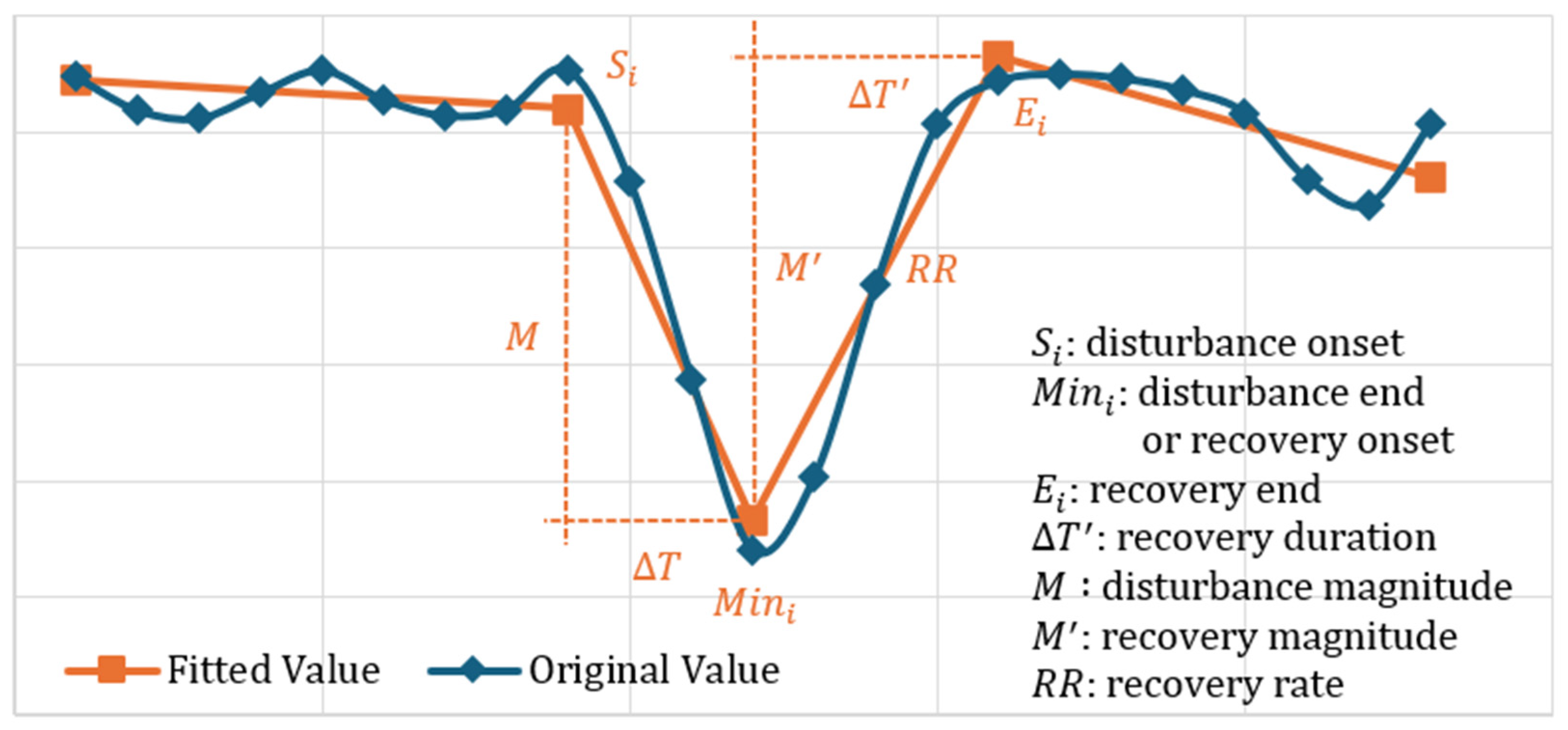
2.3.2. Disturbance and Recovery Detection
2.3.3. Multidimensional Stability Assessment
2.3.4. Assessment of Relationships among Various Stability Dimensions
2.3.5. Disturbance Result Validation Method
3. Results
3.1. Disturbance Detection
3.1.1. Disturbance Frequency
3.1.2. Maximum Disturbance Occurrence Year and Duration
3.2. Multidimensional Stability Analysis
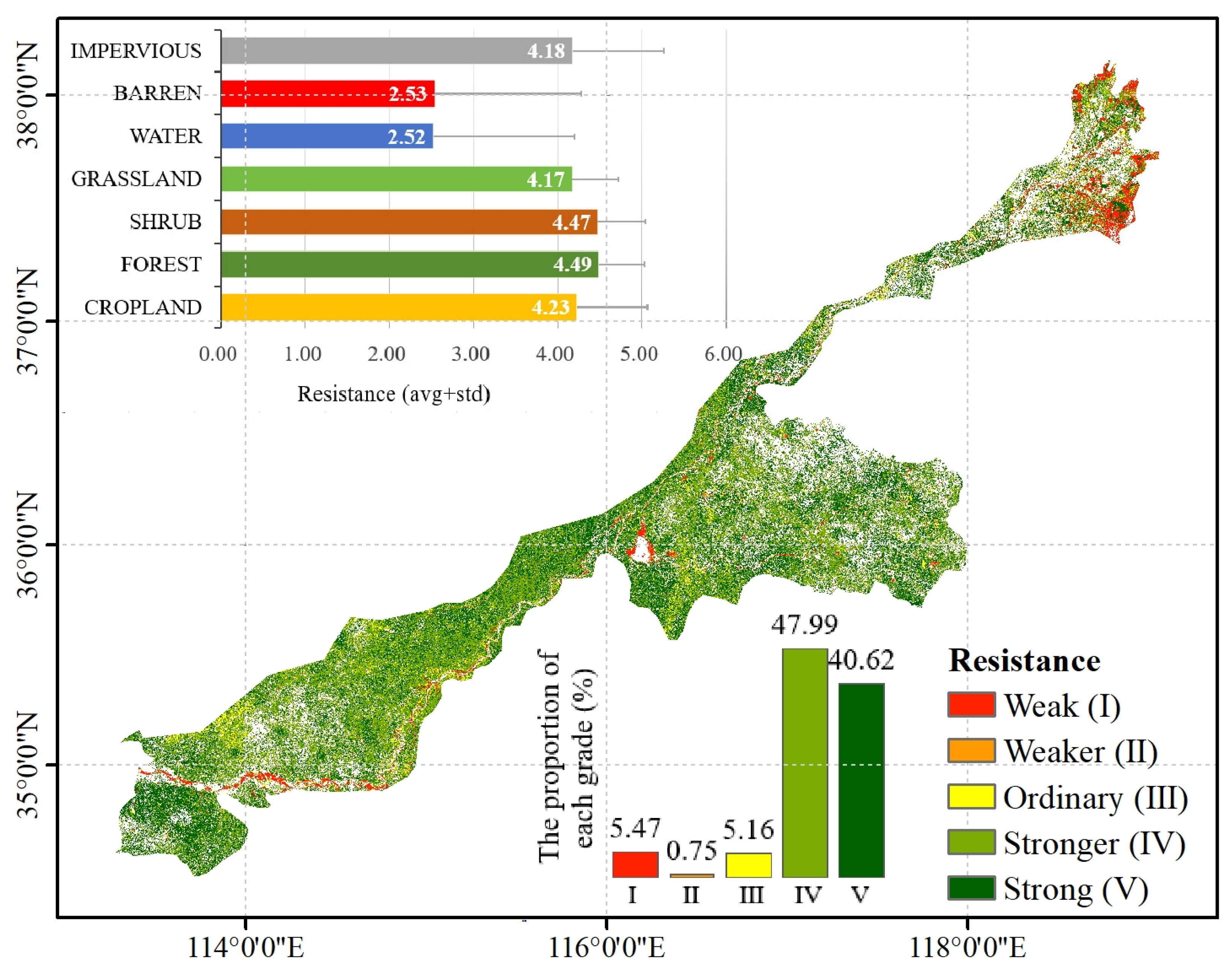
3.2.1. Resistance
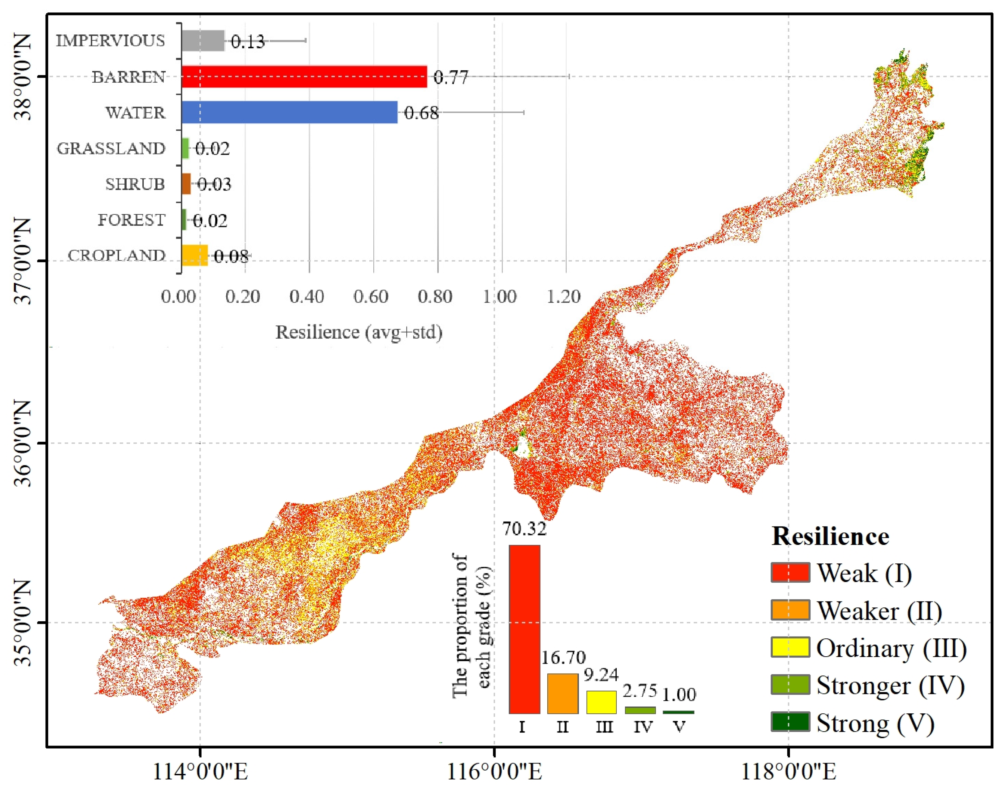
3.2.2. Resilience
3.2.3. Temporal Stability
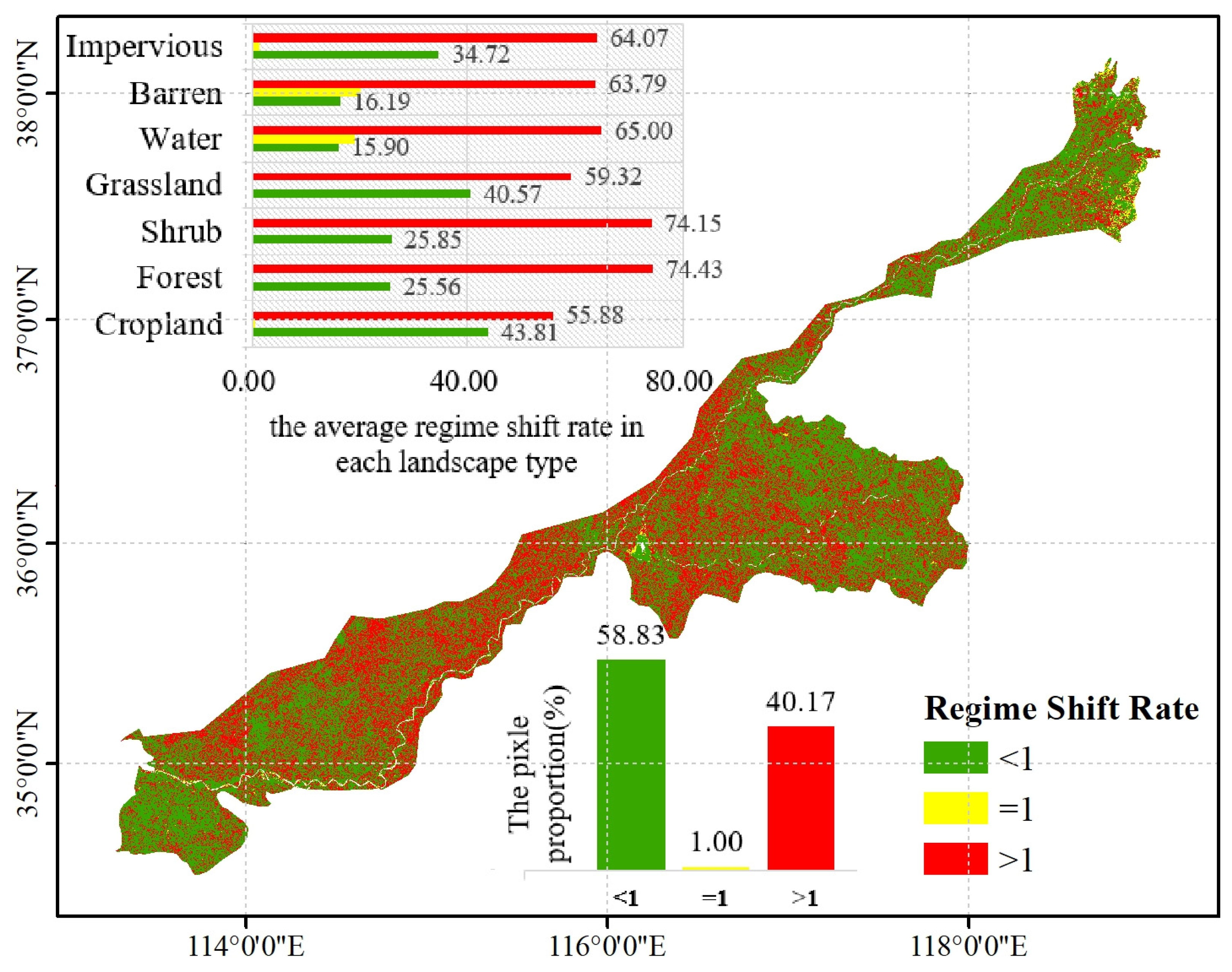
3.2.4. Regime Shift Rate
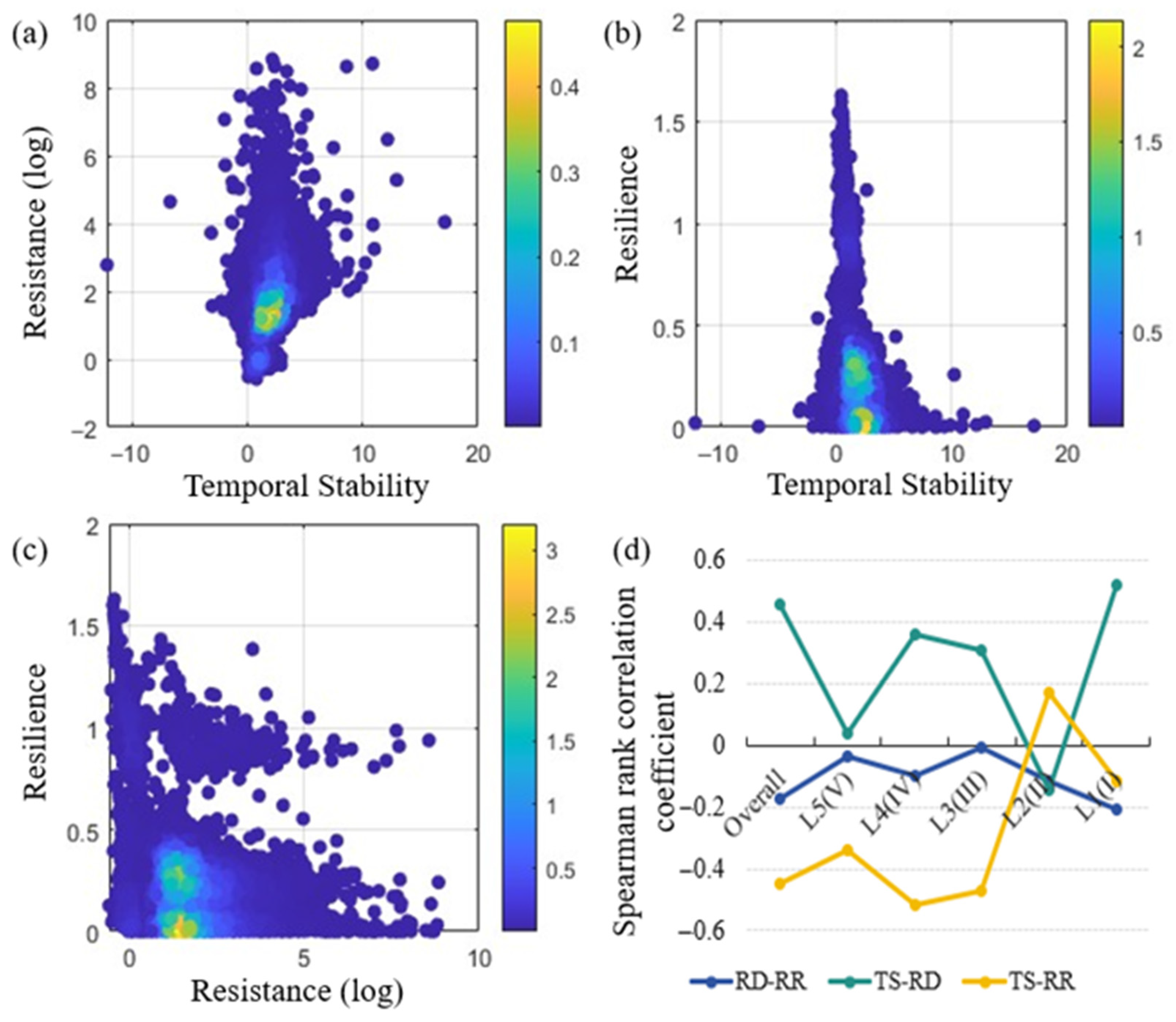
3.3. Analysis of Stability Dimensions
4. Discussion
4.1. Advantages and Uncertainties of the Assessment Framework
4.2. Rationality of Stability Assessment Results
4.2.1. Multidimensional Stability of the Ecosystem under Maximum Disturbance
4.2.2. Analysis of the Relationships between Stability Dimensions
4.2.3. Analysis of Regime Shifts and Their Significance for Ecosystem Management
4.3. Reasonability of Disturbance Detection
4.4. Other Limitations and Prospects
5. Conclusions
Supplementary Materials
Author Contributions
Funding
Data Availability Statement
Conflicts of Interest
References
- Scheffer, M.; Carpenter, S.; Foley, J.A.; Folke, C.; Walker, B. Catastrophic shifts in ecosystems. Nature 2001, 413, 591–596. [Google Scholar] [CrossRef] [PubMed]
- Donohue, I.; Hillebrand, H.; Montoya, J.M.; Petchey, O.L.; Pimm, S.L.; Fowler, M.S.; Healy, K.; Jackson, A.L.; Lurgi, M.; McClean, D.; et al. Navigating the complexity of ecological stability. Ecol. Lett. 2016, 19, 1172–1185. [Google Scholar] [CrossRef] [PubMed]
- Li, W.; Li, X.; Zhao, Y.; Zheng, S.; Bai, Y. Ecosystem structure, functioning and stability under climate change and grazing in grasslands: Current status and future prospects. Curr. Opin. Environ. Sustain. 2018, 33, 124–135. [Google Scholar] [CrossRef]
- Francesco, P.; Andreu, R. Effects of multiple stressors on the dimensionality of ecological stability. Ecol. Lett. 2021, 24, 1594–1606. [Google Scholar]
- Donohue, I.; Petchey, O.L.; Montoya, J.M.; Jackson, A.L.; McNally, L.; Viana, M.; Healy, K.; Lurgi, M.; O’Connor, N.E.; Emmerson, M.C. On the dimensionality of ecological stability. Ecol. Lett. 2013, 16, 421–429. [Google Scholar] [CrossRef]
- Kang, W.; Liu, S.; Chen, X.; Feng, K.; Guo, Z.; Wang, T. Evaluation of ecosystem stability against climate changes via satellite data in the eastern sandy area of northern China. J. Environ. Manag. 2022, 308, 114596. [Google Scholar] [CrossRef]
- Huang, Z.; Liu, X.; Yang, Q.; Meng, Y.; Zhu, L.; Zou, X. Quantifying the spatiotemporal characteristics of multi-dimensional karst ecosystem stability with Landsat time series in southwest China. Int. J. Appl. Earth Obs. Geoinf. 2021, 104, 102575. [Google Scholar] [CrossRef]
- Zhang, Y.; Liu, X.; Yang, Q.; Liu, Z.; Li, Y. Extracting Frequent Sequential Patterns of Forest Landscape Dynamics in Fenhe River Basin, Northern China, from Landsat Time Series to Evaluate Landscape Stability. Remote Sens. 2021, 13, 3963. [Google Scholar] [CrossRef]
- Eva, M.; Monika, I.; Štefan, K. The evaluation of anthropogenic impact on the ecological stability of landscape. J. Environ. Biol. 2015, 36, 1. [Google Scholar]
- Li, H.; Li, L.; Su, F.; Wang, T.; Gao, P. Ecological stability evaluation of tidal flat in coastal estuary: A case study of Liaohe estuary wetland, China. Ecol. Indic. 2021, 130, 108032. [Google Scholar] [CrossRef]
- Zhang, R.; Zhang, X.; Yang, J.; Yuan, H. Wetland ecosystem stability evaluation by using Analytical Hierarchy Process (AHP) approach in Yinchuan Plain, China. Math. Comput. Model. 2013, 57, 366–374. [Google Scholar] [CrossRef]
- Li, L.; Li, G.; Du, J.; Wu, J.; Cui, L.; Chen, Y. Effects of tidal flat reclamation on the stability of coastal wetland ecosystem services: A case study in Jiangsu Coast, China. Ecol. Indic. 2022, 145, 109697. [Google Scholar] [CrossRef]
- Tang, D.; Fan, H.; Yang, K.; Zhang, Y. Mapping forest disturbance across the China–Laos border using annual Landsat time series. Int. J. Remote Sens. 2019, 40, 2895–2915. [Google Scholar] [CrossRef]
- Yang, Y.; Erskine, P.D.; Lechner, A.M.; Mulligan, D.; Zhang, S.; Wang, Z. Detecting the dynamics of vegetation disturbance and recovery in surface mining area via Landsat imagery and LandTrendr algorithm. J. Clean. Prod. 2018, 178, 353–362. [Google Scholar] [CrossRef]
- Awty-Carroll, K.; Bunting, P.; Hardy, A.; Bell, G. Using continuous change detection and classification of Landsat data to investigate long-term mangrove dynamics in the Sundarbans region. Remote Sens. 2019, 11, 2833. [Google Scholar] [CrossRef]
- Zhu, Z.; Woodcock, C.E. Continuous change detection and classification of land cover using all available Landsat data. Remote Sens. Environ. 2014, 144, 152–171. [Google Scholar] [CrossRef]
- Li, M.; Huang, C.; Zhu, Z.; Wen, W.; Xu, D.; Liu, A. Use of remote sensing coupled with a vegetation change tracker model to assess rates of forest change and fragmentation in Mississippi, USA. Int. J. Remote Sens. 2009, 30, 6559–6574. [Google Scholar] [CrossRef]
- Huang, C.; Goward, S.N.; Masek, J.G.; Thomas, N.; Zhu, Z.; Vogelmann, J.E. An automated approach for reconstructing recent forest disturbance history using dense Landsat time series stacks. Remote Sens. Environ. 2010, 114, 183–198. [Google Scholar] [CrossRef]
- Waller, E.K.; Villarreal, M.L.; Poitras, T.B.; Nauman, T.W.; Duniway, M.C. Landsat time series analysis of fractional plant cover changes on abandoned energy development sites. Int. J. Appl. Earth Obs. Geoinf. 2018, 73, 407–419. [Google Scholar] [CrossRef]
- Verbesselt, J.; Hyndman, R.; Zeileis, A.; Culvenor, D. Phenological change detection while accounting for abrupt and gradual trends in satellite image time series. Remote Sens. Environ. 2010, 114, 2970–2980. [Google Scholar] [CrossRef]
- Ding, H.; Yuan, Z.; Yin, J.; Shi, X.; Shi, M. Evaluating ecosystem stability based on the dynamic time warping algorithm: A case study in the Minjiang river Basin, China. Ecol. Indic. 2023, 154, 110501. [Google Scholar] [CrossRef]
- Griffiths, P.; Kuemmerle, T.; Kennedy, R.E.; Abrudan, I.V.; Knorn, J.; Hostert, P. Using annual time-series of Landsat images to assess the effects of forest restitution in post-socialist Romania. Remote Sens. Environ. 2012, 118, 199–214. [Google Scholar] [CrossRef]
- Kennedy, R.E.; Yang, Z.; Braaten, J.; Copass, C.; Antonova, N.; Jordan, C.; Nelson, P. Attribution of disturbance change agent from Landsat time-series in support of habitat monitoring in the Puget Sound region, USA. Remote Sens. Environ. 2015, 166, 271–285. [Google Scholar] [CrossRef]
- Fu, B.; Lan, F.; Xie, S.; Liu, M.; He, H.; Li, Y.; Liu, L.; Huang, L.; Fan, D.; Gao, E.; et al. Spatio-temporal coupling coordination analysis between marsh vegetation and hydrology change from 1985 to 2019 using LandTrendr algorithm and Google Earth Engine. Ecol. Indic. 2022, 137, 108763. [Google Scholar] [CrossRef]
- Shen, Q.; Gao, G.; Duan, Y.; Chen, L. Long-term continuous changes of vegetation cover in desert oasis of a hyper-arid endorheic basin with LandTrendr algorithm. Ecol. Indic. 2024, 166, 112418. [Google Scholar] [CrossRef]
- Fu, B.; Chen, L.; Wang, J.; Meng, Q.; Zhao, W. Land use structure and ecological processes. Quat. Sci. 2003, 23, 247–256. [Google Scholar]
- Yu, G.; Wang, Y.; Yang, M. Discussion on the ecological theory and technological approaches of ecosystem quality improvement and stability enhancement. Chin. J. Appl. Ecol. 2023, 34, 1–10. [Google Scholar] [CrossRef]
- Tamiminia, H.; Salehi, B.; Mahdianpari, M.; Quackenbush, L.; Adeli, S.; Brisco, B. Google Earth Engine for geo-big data applications: A meta-analysis and systematic review. ISPRS J. Photogramm. Remote Sens. 2020, 164, 152–170. [Google Scholar] [CrossRef]
- Simonetti, D.; Simonetti, E.; Szantoi, Z.; Lupi, A.; Eva, H.D. First Results From the Phenology-Based Synthesis Classifier Using Landsat 8 Imagery. IEEE Geosci. Remote Sens. Lett. 2015, 12, 1496–1500. [Google Scholar] [CrossRef]
- Roy, D.P.; Kovalskyy, V.; Zhang, H.; Vermote, E.F.; Yan, L.; Kumar, S.; Egorov, A. Characterization of Landsat-7 to Landsat-8 reflective wavelength and normalized difference vegetation index continuity. Remote Sens. Environ. 2016, 185, 57–70. [Google Scholar] [CrossRef]
- Zhang, J.; Du, J.; Fang, S.; Sheng, Z.; Zhang, Y.; Sun, B.; Mao, J.; Li, L. Dynamic changes, spatiotemporal differences, and ecological effects of impervious surfaces in the Yellow river basin, 1986–2020. Remote Sens. 2023, 15, 268. [Google Scholar] [CrossRef]
- Yang, J.; Huang, X. The 30 m annual land cover dataset and its dynamics in China from 1990 to 2019. Earth Syst. Sci. Data 2021, 13, 3907–3925. [Google Scholar] [CrossRef]
- Zhang, Y.; Du, J.; Guo, L.; Fang, S.; Zhang, J.; Sun, B.; Mao, J.; Sheng, Z.; Li, L. Long-term detection and spatiotemporal variation analysis of open-surface water bodies in the Yellow River Basin from 1986 to 2020. Sci. Total Environ. 2022, 845, 157152. [Google Scholar] [CrossRef]
- Pekel, J.F.; Cottam, A.; Gorelick, N.; Belward, A. High-resolution mapping of global surface water and its long-term changes. Nature 2016, 540, 418–422. [Google Scholar] [CrossRef]
- Xu, H.; Wang, M.; Shi, T.; Guan, H.; Fang, C.; Lin, Z. Prediction of ecological effects of potential population and impervious surface increases using a remote sensing based ecological index (RSEI). Ecol. Indic. 2018, 93, 730–740. [Google Scholar] [CrossRef]
- Camps-Valls, G.; Campos-Taberner, M.; Moreno-Martínez, Á.; Walther, S.; Duveiller, G.; Cescatti, A.; Mahecha, M.D.; Muñoz-Marí, J.; García-Haro, F.J.; Guanter, L. A unified vegetation index for quantifying the terrestrial biosphere. Sci. Adv. 2021, 7, eabc7447. [Google Scholar] [CrossRef]
- Haralick, R.M.; Shanmugam, K.; Dinstein, I.H. Textural features for image classification. IEEE Trans. Syst. Man Cybern. 1973, SMC-3, 610–621. [Google Scholar] [CrossRef]
- Kennedy, R.E.; Yang, Z.; Cohen, W.B. Detecting trends in forest disturbance and recovery using yearly Landsat time series: 1. LandTrendr—Temporal segmentation algorithms. Remote Sens. Environ. 2010, 114, 2897–2910. [Google Scholar] [CrossRef]
- Kéfi, S.; Domínguez-García, V.; Donohue, I.; Fontaine, C.; Thébault, E.; Dakos, V. Advancing our understanding of ecological stability. Ecol. Lett. 2019, 22, 1349–1356. [Google Scholar] [CrossRef]
- White, H.J.; Gaul, W.; Sadykova, D.; León-Sánchez, L.; Caplat, P.; Emmerson, M.C.; Yearsley, J.M. Quantifying large-scale ecosystem stability with remote sensing data. Remote Sens. Ecol. Conserv. 2020, 6, 354–365. [Google Scholar] [CrossRef]
- Smith, T.; Boers, N. Reliability of vegetation resilience estimates depends on biomass density. Nat. Ecol. Evol. 2023, 7, 1799–1808. [Google Scholar] [CrossRef]
- Liu, M.; Liu, X.; Wu, L.; Tang, Y.; Li, Y.; Zhang, Y.; Ye, L.; Zhang, B. Establishing forest resilience indicators in the hilly red soil region of southern China from vegetation greenness and landscape metrics using dense Landsat time series. Ecol. Indic. 2021, 121, 106985. [Google Scholar] [CrossRef]
- Hermosilla, T.; Wulder, M.A.; White, J.C.; Coops, N.C.; Hobart, G.W. Regional detection, characterization, and attribution of annual forest change from 1984 to 2012 using Landsat-derived time-series metrics. Remote Sens. Environ. 2015, 170, 121–132. [Google Scholar] [CrossRef]
- Hamunyela, E.; Verbesselt, J.; Herold, M. Using spatial context to improve early detection of deforestation from Landsat time series. Remote Sens. Environ. 2016, 172, 126–138. [Google Scholar] [CrossRef]
- Zhu, Z. Change detection using landsat time series: A review of frequencies, preprocessing, algorithms, and applications. ISPRS J. Photogramm. Remote Sens. 2017, 130, 370–384. [Google Scholar] [CrossRef]
- Meng, Y.; Liu, X.; Ding, C.; Xu, B.; Zhu, L. Analysis of ecological resilience to evaluate the inherent maintenance capacity of a forest ecosystem using a dense Landsat time series. Ecol. Inform. 2020, 57, 101064. [Google Scholar] [CrossRef]
- Hillebrand, H.; Langenheder, S.; Lebret, K.; Lindström, E.; Östman, Ö.; Striebel, M. Decomposing multiple dimensions of stability in global change experiments. Ecol. Lett. 2017, 21, 21–30. [Google Scholar] [CrossRef]
- Li, X.; Piao, S.; Wang, K.; Wang, X.; Wang, T.; Ciais, P.; Chen, A.; Lian, X.; Peng, S.; Peñuelas, J. Temporal trade-off between gymnosperm resistance and resilience increases forest sensitivity to extreme drought. Nat. Ecol. Evol. 2020, 4, 1075–1083. [Google Scholar] [CrossRef]
- Shi, X.; Chen, F.; Ding, H.; Shi, M.; Li, Y. Assessing Vegetation Ecosystem Resistance to Drought in the Middle Reaches of the Yellow River Basin, China. Int. J. Environ. Res. Public Health 2022, 19, 4180. [Google Scholar] [CrossRef]
- Scheffer, M.; Carpenter, S.R. Catastrophic regime shifts in ecosystems: Linking theory to observation. Trends Ecol. Evol. 2003, 18, 648–656. [Google Scholar] [CrossRef]
- Chen, J.; Chi, Y.; Zhou, W.; Wang, Y.; Zhuang, J.; Zhao, N.; Ding, J.; Song, J.; Zhou, L. Quantifying the dimensionalities and drivers of ecosystem stability at global scale. J. Geophys. Res. Biogeosci. 2021, 126, e2020JG006041. [Google Scholar] [CrossRef]
- Xu, Z.; Ren, H.; Li, M.H.; van Ruijven, J.; Han, X.; Wan, S.; Li, H.; Yu, Q.; Jiang, Y.; Jiang, L. Environmental changes drive the temporal stability of semi-arid natural grasslands through altering species asynchrony. J. Ecol. 2015, 103, 1308–1316. [Google Scholar] [CrossRef]
- De Keersmaecker, W.; Lhermitte, S.; Tits, L.; Honnay, O.; Somers, B.; Coppin, P. A model quantifying global vegetation resistance and resilience to short-term climate anomalies and their relationship with vegetation cover. Glob. Ecol. Biogeogr. 2015, 24, 539–548. [Google Scholar] [CrossRef]
- Geng, S.; Shi, P.; Song, M.; Zong, N.; Zu, J.; Zhu, W. Diversity of vegetation composition enhances ecosystem stability along elevational gradients in the Taihang Mountains, China. Ecol. Indic. 2019, 104, 594–603. [Google Scholar] [CrossRef]
- Valerio, F.; Godinho, S.; Marques, A.T.; Crispim-Mendes, T.; Pita, R.; Silva, J.P. GEE_xtract: High-quality remote sensing data preparation and extraction for multiple spatio-temporal ecological scaling. Ecol. Inform. 2024, 80, 102502. [Google Scholar] [CrossRef]
- Padilla, M.; Wheeler, J.; Tansey, K. ESA Climate Change Initiative–Fire_cci D4. 1.1 Product Validation Report (PVR); Universidad de Alcala: Madrid, Spain, 2018. [Google Scholar]
- Tellman, B.; Sullivan, J.A.; Kuhn, C.; Kettner, A.J.; Doyle, C.S.; Brakenridge, G.R.; Erickson, T.A.; Slayback, D.A. Satellite imaging reveals increased proportion of population exposed to floods. Nature 2021, 596, 80–86. [Google Scholar] [CrossRef] [PubMed]
- Beguería, S.; Vicente Serrano, S.M.; Reig-Gracia, F.; Latorre Garcés, B. SPEIbase v. 2.9 [Dataset]. 2023. Available online: https://digital.csic.es/handle/10261/332007 (accessed on 12 February 2024).
- Crist, E.P. A TM tasseled cap equivalent transformation for reflectance factor data. Remote Sens. Environ. 1985, 17, 301–306. [Google Scholar] [CrossRef]
- Baig, M.H.A.; Zhang, L.; Shuai, T.; Tong, Q. Derivation of a tasselled cap transformation based on Landsat 8 at-satellite reflectance. Remote Sens. Lett. 2014, 5, 423–431. [Google Scholar] [CrossRef]
- Artis, D.A.; Carnahan, W.H. Survey of emissivity variability in thermography of urban areas. Remote Sens. Environ. 1982, 12, 313–329. [Google Scholar] [CrossRef]
- Sekertekin, A.; Bonafoni, S. Land surface temperature retrieval from Landsat 5, 7, and 8 over rural areas: Assessment of different retrieval algorithms and emissivity models and toolbox implementation. Remote Sens. 2020, 12, 294. [Google Scholar] [CrossRef]
- Kumar, D.; Soni, A.; Kumar, M. Retrieval of land surface temperature from landsat-8 thermal infrared sensor data. J. Hum. Earth Future 2022, 3, 159–168. [Google Scholar] [CrossRef]
- XU, H.-Q. A new index-based built-up index (IBI) and its eco-environmental significance. Remote Sens. Technol. Appl. 2011, 22, 301–308. [Google Scholar]


| Parameter | Value | Parameter | Value |
|---|---|---|---|
| Max Segments | 12 | recoveryThreshold | 0.5 |
| Spike Threshold | 0.95 | pvalThreshold | 0.1 |
| Vertex Count Overshoot | 3 | bestModelProportion | 0.75 |
| Prevent One Year Recovery | False | minObservationsNeeded | 6 |
| Stability Component | Expression | Explanation |
|---|---|---|
| Resistance (RD) | RD = 1/M | Resistance reflects an ecosystem’s ability to absorb disturbances, with the core concept being the capacity to “resist disturbances and maintain its original state.” It is quantified as the inverse of an ecosystem’s deviation from its equilibrium state following a disturbance [39]. A higher resistance value indicates a more stable system. |
| Resilience (RR) | RR = M’/ΔT’ | Resilience refers to an ecosystem’s ability to recover to a stable state after being disturbed, with a core concept of “damaged but returning to its original state”. It is quantified as the ratio of the magnitude of changes in ecosystem parameters to the recovery time once the disturbance has been eliminated [40]. A higher resilience indicates a more stable system. |
| Temporal Stability (TS) | TS = 1/cv = μ/σ | Evaluated using the reciprocal of the coefficient of variation (cv), where μ is the mean value of the characteristic parameter, and σ is the standard deviation. The greater the temporal stability, the more stable the system. |
| Regime shift rate (RS) | RS = M/M’ | Described by the ratio of the magnitude of disturbance to the magnitude of recovery [21]. This index can determine the direction of a regime shift. |
| Level | Weak (I) | Weaker (II) | Ordinary (III) | Stronger (IV) | Strong (V) |
|---|---|---|---|---|---|
| D | ≤1.25 | (1.25, 1.67] | (1.67, 2.5] | (2.5, 5] | >5 |
| RR | ≤0.2 | (0.2, 0.4] | (0.4, 0.6] | (0.6, 0.8] | >0.8 |
| TS | ≤1 | (1, 2] | (2, 3] | (3, 4] | >4 |
Disclaimer/Publisher’s Note: The statements, opinions and data contained in all publications are solely those of the individual author(s) and contributor(s) and not of MDPI and/or the editor(s). MDPI and/or the editor(s) disclaim responsibility for any injury to people or property resulting from any ideas, methods, instructions or products referred to in the content. |
© 2024 by the authors. Licensee MDPI, Basel, Switzerland. This article is an open access article distributed under the terms and conditions of the Creative Commons Attribution (CC BY) license (https://creativecommons.org/licenses/by/4.0/).
Share and Cite
Li, L.; Du, J.; Wu, J.; Sheng, Z.; Zhu, X.; Song, Z.; Zhai, G.; Chong, F. Evaluating the Multidimensional Stability of Regional Ecosystems Using the LandTrendr Algorithm. Remote Sens. 2024, 16, 3762. https://doi.org/10.3390/rs16203762
Li L, Du J, Wu J, Sheng Z, Zhu X, Song Z, Zhai G, Chong F. Evaluating the Multidimensional Stability of Regional Ecosystems Using the LandTrendr Algorithm. Remote Sensing. 2024; 16(20):3762. https://doi.org/10.3390/rs16203762
Chicago/Turabian StyleLi, Lijuan, Jiaqiang Du, Jin Wu, Zhilu Sheng, Xiaoqian Zhu, Zebang Song, Guangqing Zhai, and Fangfang Chong. 2024. "Evaluating the Multidimensional Stability of Regional Ecosystems Using the LandTrendr Algorithm" Remote Sensing 16, no. 20: 3762. https://doi.org/10.3390/rs16203762