Article

On the Suitability of Different Satellite Land Surface Temperature Products to Study Surface Urban Heat Islands

by
Alexandra Hurduc
1,*,
Sofia L. Ermida
1,2 and
Carlos C. DaCamara
1
1
Instituto Dom Luiz (IDL), Faculdade de Ciências, Universidade de Lisboa, 1749-016 Lisbon, Portugal
2
Instituto Português do Mar e da Atmosfera (IPMA), 1749-077 Lisbon, Portugal
*
Author to whom correspondence should be addressed.
Remote Sens. 2024, 16(20), 3765; https://doi.org/10.3390/rs16203765
Submission received: 30 July 2024 / Revised: 2 October 2024 / Accepted: 8 October 2024 / Published: 10 October 2024
(This article belongs to the Section AI Remote Sensing)

Abstract

:
Remote sensing satellite data have been a crucial tool in understanding urban climates. The variety of sensors with different spatiotemporal characteristics and retrieval methodologies gave rise to a multitude of approaches when analyzing the surface urban heat island effect (SUHI). Although there are considerable advantages that arise from these different characteristics (spatiotemporal resolution, time of observation, etc.), it also means that there is a need for understanding the ability of sensors in capturing spatial and temporal SUHI patterns. For this, several land surface temperature products are compared for the cities of Madrid and Paris, retrieved from five sensors: the Spinning Enhanced Visible and InfraRed Imager onboard Meteosat Second Generation, the Advanced Very-High-Resolution Radiometer onboard Metop, the Moderate-resolution Imaging Spectroradiometer onboard both Aqua and Terra, and the Thermal Infrared Sensor onboard Landsat 8 and 9. These products span a wide range of LST algorithms, including split-window, single-channel, and temperature–emissivity separation methods. Results show that the diurnal amplitude of SUHI may not be well represented when considering daytime and nighttime polar orbiting platforms. Also, significant differences arise in SUHI intensity and spatial and temporal variability due to the different methods implemented for LST retrieval.

1. Introduction

Remote sensing data have been widely used in the past decades for the study of urban climate [1,2,3,4,5,6,7,8]. In addition to the long archives of repeated observations, the global coverage offered by these datasets are an added advantage when compared with in situ observations, while being available in various temporal and spatial resolutions [9,10]. Free access to these data has promoted an increase in urban climate studies, with consideration to the rising percentage of populations residing in cities [11]. One of the major concerns when discussing urban climate is the urban heat island effect, consisting in the difference in temperature between urban and surrounding non-urban areas [12]. Surface urban heat islands (SUHIs) have particular relevance, as a temperature increase directly affects population health and comfort and can be derived for the whole globe [13,14,15,16,17,18]. Two of the most broadly used orbits in meteorology/climate are polar and geostationary orbits. Polar orbit (PO) platforms are low-orbiting, enabling a spatial resolution from a km to a few tenths of meters, with a revisit time of twice daily to 16 days. On the other hand, geostationary satellites, with a higher orbit, have a coarser spatial resolution, of the order of a few kilometers at the sub-satellite point, while having sub-hourly sampling times [19,20]. As land surface temperature (LST) is derived from measurements in the thermal infrared part of the electromagnetic spectrum [21], cloud coverage usually decreases the availability of observations, hindering the use of satellite LST in cloudy conditions, except for microwave-derived LST [22,23]. Different spatiotemporal characteristics are better suited for different research topics. For example, polar orbiting satellites have a greater advantage compared to geostationary ones in circumstances where the finer spatial resolution is particularly relevant. Topics where better spatial resolution is preferred can relate to analyzing vegetation growth/health, heat waves, natural disasters, etc. [24,25,26,27]. On the other hand, geostationary satellites are better suited to the study of diurnal cycles due to their higher sampling rate, enabling a better representation of, for instance, the daily temperature amplitude [28,29,30,31,32]. A majority of remote sensing SUHI studies rely on polar orbiting satellites [9,10,33,34,35]. These studies have greatly improved understanding of SUHI, especially its trends and seasonal variability. Works based on these sensors have also analyzed the diurnal cycle of SUHI, however, with few daily observations (relying on only two to four observations, during clear sky conditions) [9,36]. Although useful, this approach does not give a comprehensive understanding of surface variables’ complexity [10,37]. As the revisit time of polar orbiting sensors may not be enough to characterize SUHIs’ diurnal cycle, geostationary satellites have been used to combat this limitation [38,39,40,41,42,43]. These studies have found added value when considering more observations per day even at the cost of coarser spatial resolution. Some work has already been carried out in downscaling LST from geostationary sensors, in order to have a better understanding of both temporal and spatial variability in SUHI [41,44,45,46].
Furthermore, methodologies to derive LST from satellite observations are also very diverse [47,48]. The most widely used, and considered most accurate, are the so-called split-window algorithms, which derive LST by considering the differential absorption between adjacent channels in the thermal infrared atmospheric window [47,48,49,50]. The current operational LST products derived within the Satellite Application Facility on Land Surface Analysis (LSA-SAF) for the Spinning Enhanced Visible and InfraRed Imager (SEVIRI) and Advanced Very-High-Resolution Radiometer (AVHRR) sensors are based on the generalized split-window (GSW) algorithm [50,51]. The Moderate-resolution Imaging Spectroradiometer (MODIS) Land Surface Temperature/Emissivity product (MOD11/MYD11) is also based on the GSW but refined to include a quadratic term [52]. Split-window algorithms require prescribed values of land surface emissivity and are very sensitive to those values [53,54,55]. There are also a wide range of methodologies used to derive the surface emissivity, and these may have a significant impact on LST retrieval particularly in the case of cities, given the high heterogeneity of surface materials [56,57,58]. In this case, all three considered split-window products (SEVIRI, AVHRR, and MODIS) use land cover classification to derive emissivity, resulting in a single value being attributed to all urban surfaces, which likely results in an underrepresentation of the variability in the different materials used in urban construction [59]. The attributed value is therefore highly sensitive to the spectral library data considered. In these cases, the quality of the surface emissivity is also dependent on the quality of the land cover classification.
To circumvent the need to prescribe the surface emissivity, a method that has been widely used in the past decade is the temperature–emissivity separation (TES) algorithm. This algorithm uses an empirical relationship between the maximum emissivity spectral contrast and the minimum emissivity, which allows for simultaneously retrieving LST and emissivity [60,61,62]. However, some studies suggest that the current calibration of this empirical relationship might not be appropriate for man-made materials [63,64].
In the case of the Landsat series, only the most recent Landsat 9 provides the dual thermal infrared bands necessary to apply a split-window algorithm, due to problems in the sensor of Landsat 8 [65]. Available products are, therefore, based on single-channel methods [47,48]. The current operational Landsat Collection 2 Surface Temperature Science Product applies a radiative transfer model to obtain the LST [66,67]. We also analyze the freely available Landsat LST estimates derived in [68] that are based on the Statistical Mono-Window algorithm [28]. In both cases, the emissivity is prescribed based on the Advanced Spaceborne Thermal Emission and Reflection Radiometer (ASTER) Global Emissivity Database (GED) [69] and using the Normalized Difference Vegetation Index (NDVI) to account for vegetation dynamics [70,71,72].
Given the high heterogeneity of LST products, both in terms of the retrieval algorithm and spatiotemporal availability, here, we aim to understand the impact of the LST product selection when analyzing the SUHI effect in two cities, Madrid and Paris, throughout the 2015–2023 period. For that purpose, we will consider the temporal and spatial resolutions of the different sensors, while also providing comparisons between LST retrievals derived by the different algorithms. Section 2 provides a summary of the data and methods. Results are shown in Section 3 and discussed in Section 4. Conclusions are given in Section 5.

2. Materials and Methods

The current work focuses on two cities: Madrid and Paris. These were chosen for, firstly, being large enough to be detected by both polar orbiting and geostationary sensors and secondly, for being cities already approached in previous SUHI studies (e.g., [35,38]). Madrid is the capital of Spain, also being the country’s largest city. It is located in a mainly flat area except for the Spanish Central Ridge to the north. The city’s climate is a temperate Mediterranean one, with cool winters and hot summers. These are also the driest seasons, with most of the rainfall concentrating in spring and fall [73]. Paris, the capital of France, is located in the north-center area of the country in a valley-like orientation, being relatively smooth with altitudes no higher than 230 m above sea level. The region is characterized by hot summers and mild winters [74,75]. More information on the climate, topography, and demographics of these cities can be found elsewhere [76,77]. The two cities were selected for representing very different SUHI patterns, with Madrid typically presenting a more intense SUHI during the nighttime, while Paris is characterized by a typical daytime SUHI [35,78,79,80,81,82,83]. The period ranging from 2015 to 2023 was considered in order to encompass all selected satellite sensors.

2.1. Data

In this work, a wide range of LST products was considered. The product selection aims at increasing the diversity in temporal sampling, overpass time, spatial resolution, and LST algorithm. Five sensors were considered: the SEVIRI onboard the Meteosat Second Generation (MSG) series, the AVHRR onboard the Metop series, the MODIS onboard both Aqua and Terra, and the Thermal Infrared Sensor (TIRS and TIRS-2) onboard Landsat 8 and 9. A total of eight products were used. A summary of their characteristics can be found in Table 1.
The MLST product is provided by the LSA SAF and is derived from observations by SEVIRI onboard the MSG satellites, in a geostationary orbit. Data correspond to operational monthly means at different times of the day (with a frequency of 15 min), at a resolution of 0.05° in latitude and longitude [51].
The EDLST product is also provided by the LSA SAF. It is based on measurements by the AVHRR sensor onboard the Metop polar orbiting series of satellites. The product is available twice daily (day/night) at a 0.01° resolution in latitude and longitude [84]. The equatorial crossing time (ECT) of the Metop satellites is around 9:30 a.m./p.m. (local time).
MODIS is a sensor onboard the polar orbiting Terra and Aqua platforms, also available twice daily (day/night) for each. Two products were used for each platform, resulting in a total of four LST products, MYD11A1 v061, MOD11A1 v061, MYD21A1D and MYD12A1N v061, and MOD21A1D and MOD21A1N v061, hereafter mentioned as MYD11, MOD11, MYD21, and MOD21, respectively. The ECT of the Aqua satellite (and therefore of the MYD11 and MYD21 products) is approximately 1:30 a.m./p.m., while the ECT of the Terra satellite (products MOD11 and MOD21) is around 10:30 a.m./p.m. All MODIS products were downloaded through the Application for Extracting and Exploring Analysis-Ready Samples (AρρEEARS NASA, https://appeears.earthdatacloud.nasa.gov, accessed on 1 June 2024), on a geographic WGS84 projection.
Landsat LST is based on the TIRS and TIRS-2 sensors onboard Landsat 8 and 9, respectively, with a revisit time of 16 days. The Landsat satellites have a ECT of approximately 11:00 a.m./p.m. Two products were considered: GEE Landsat LST [68] was retrieved at a 30 m spatial resolution using the Google Earth Engine platform. USGS LST data were downloaded through the USGS Earth Explorer tool (https://earthexplorer.usgs.gov, accessed on 1 June 2024), corresponding to the full tile covering each city with a 30 m resolution.
The Copernicus CGLS-LC100 v3.0.1 product was used to identify urban (buildup) and rural (tree, shrub, grass, crop) areas and corresponds to the 2015–2019 period with a 100 m resolution [89].

2.2. Methods

Products were assessed based on both LST and SUHI. SUHI intensity was computed as the difference between the temperature of the urban area and the rural one, as shown in expression (1).
SUHI = LSTUrban − LSTRural
For simplicity, in this work, we use the term “SUHI” to address the SUHI intensity as defined in Equation (1). For distinguishing between urban and rural pixels, the CGLS-LC100 product was used and resampled to the projection of each LST product, as depicted in Figure 1. Only pixels containing a minimum of 80% of urban (buildup) or rural (tree, shrub, grass, crop) areas were considered. For MLST, EDLST, and MxDx1 products, the 100 m land cover (LC) statistical mode was attributed to each LST coarse pixel. For Landsat-derived products, a nearest-neighbor interpolation was used to resample LC to the LST spatial grid. The size of the geographical area considered for each city was chosen to balance, as far as possible, the ratio between urban and rural pixels for each sensor. The percentage of urban LC in each resampled pixel is also shown in Figure 1.
The assessment presented in this study is performed using monthly mean values of the LSTs. This allows a better representation of the SUHI/LST diurnal maximum/minimum values in the case of the MLST product, as these may be severely affected by the availability of data at the times of these maximum/minimum values due to cloud cover. For the remaining products (EDLST, MxDx1, GEE/USGS Landsat), the respective day/night monthly mean values are also computed. For EDLST and MxDx1, only instants that have more than 70% of valid pixels within the interest region are considered, ensuring a consistent representation of urban and rural pixels. This process was not applied to MLST as the products already consist of mean monthly temperatures, nor for the GEE/USGS Landsat products as it resulted in a large part of the months being discarded. Seasonal means are then computed from the monthly mean values.
For inter-comparison purposes, and in order to identify potential bias between products due to differences in methodologies of retrieval, all products were also resampled onto the 0.05° projection of the MLST product. All polar orbit products (EDLST, MxDx1, Landsat) were then compared against the MLST observations at the respective observation times of the polar satellites. Polar orbiters with similar observation times were also inter-compared, namely combining EDLST, MOD11, MOD21, GEE Landsat, and USGS LST in a morning observation group and MYD11 and MYD21 in an afternoon observation group. All comparisons were performed at the level of the monthly mean values.

3. Results

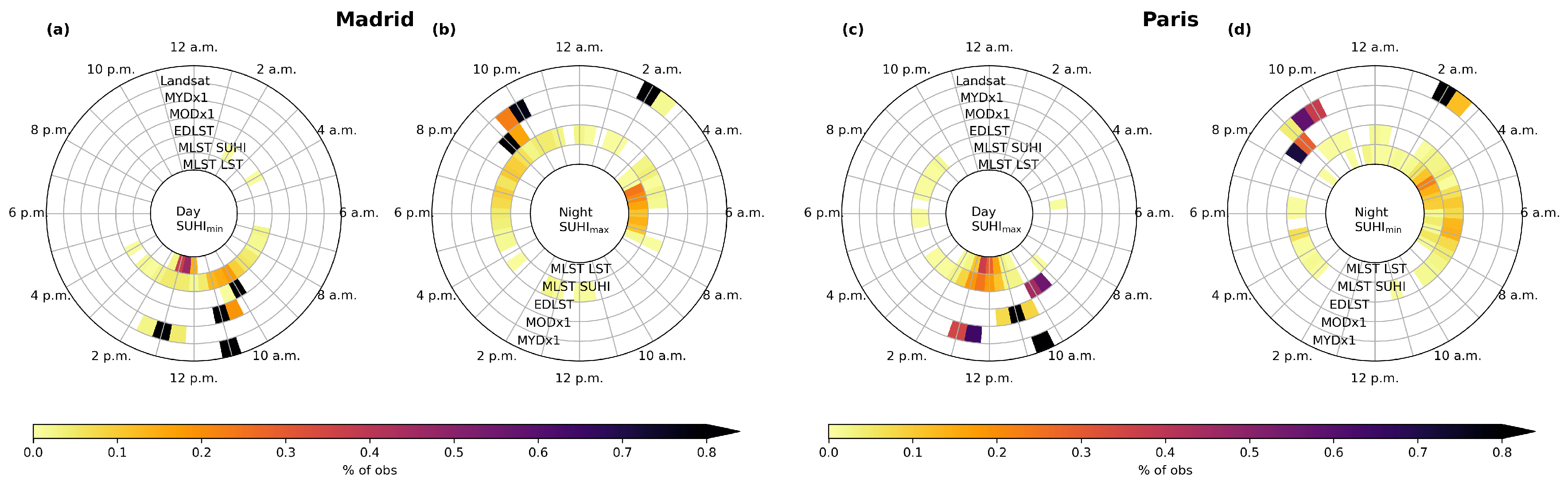
3.1. Observation Time

Sensors onboard polar orbiting satellites maintain the same observation time all year. As the time of day when minimum and maximum surface temperatures occur can slightly shift throughout the year, measuring the LST at a constant time throughout the year may lead to an incomplete characterization of its diurnal amplitude. Also, as LST is highly influenced by the seasonality of incoming solar radiation, it also follows a seasonal cycle. LST of surfaces with different physical characteristics (e.g., heat conductivity, albedo, and emissivity) have different heating and cooling rates [5], meaning that computing the difference between the temperature of an urban/artificial surface and a rural/natural one at the same time of day throughout the year might be misleading in terms of the minimum, maximum, and amplitude of the SUHI.
To understand the potential impact of using a satellite product with a fixed overpass time, Figure 2 shows the observation time of each of the sensors considered. The figure also shows times of minimum and maximum values of LST (MLST LST) and SUHI (MLST SUHI) as obtained from the MLST dataset. Since Madrid and Paris have very distinct SUHI behaviors, with Madrid having a more intense SUHI during the night and Paris during the day, daytime (nighttime) observations are grouped together with the times of the SUHI minimum (maximum) in the case of Madrid (Figure 2a,b) and with the times of the SUHI maximum (minimum) in the case of Paris (Figure 2c,d). Although polar orbit satellites have approximately fixed ECT, the actual observation time at different locations may change slightly from day to day due to shifts in the orbit position and possible overlap between orbits, especially in the case of sensors with wide swaths such as MODIS and AVHRR.
In the case of Madrid observations (Figure 2a,b), Landsat shows the smallest range of observation times, with values around 11:00 a.m. The Aqua products (MYDx1) have observations between 12:30 and 1:45 p.m. (1:45 and 2:45 a.m.), and the Terra ones (MODx1) between 10:15 and 11:15 a.m. (9:15 and 10:15 p.m.). The EDLST product has observations between 9:45 and 10:45 a.m. (8:45 and 0:45 p.m.) during daytime (nighttime). The time of the LST maximum (minimum) in the city of Madrid occurs between 11:45 and 1:45 p.m. (3:15 and 7:45 a.m.), based on the MLST product. The time of minimum SUHI (Figure 2a) shows a much wider range, from about 7:45 a.m. to 4:15 p.m., with the most frequent values occurring around 9:15–11:15 a.m. The range of maximum SUHI (Figure 2b) is particularly large, spanning almost all day, with a main cluster around 4:15–11:15 p.m. (with highest frequency around 6:15–8:45 p.m.) and two secondary ones around 11:45 a.m.–2:15 p.m. and 3:15–5:45 a.m.
For daytime observations over Paris (Figure 2c), Landsat products also show the smallest range of observation times, with values around 10:30 a.m. Daytime (nighttime) observations over Paris (Figure 2c,d) of the MYDx1, MODx1, and EDLST occur between 12:15 and 13:15 p.m. (1:45 and 2:45 a.m.), 10:15 and 11:45 a.m. (8:45 and 10:15 p.m.), and 9:15 and 10:15 a.m. (8:15 and 9:15 p.m.), respectively. Based on the MLST product, the maximum of LST (Figure 2c) occurs around 10:15 a.m.–2:15 p.m. and the minimum (Figure 2d) shows a significantly higher spread, occurring between 11:15 and 8:15 a.m. and with higher frequency around 2:00–6:00 a.m. In Paris, the time of the SUHI maximum (Figure 2c) shows a main cluster around 10:15 a.m. to 3:45 p.m. with higher frequency around 11:15 a.m.–2:00 p.m., and a secondary cluster around 5:00–9:00 p.m. The SUHI minimum (Figure 2d) also shows a particularly large range of times, having a main cluster around 2:15–9:45 a.m. with higher frequencies at 5:00–8:00 a.m., and secondary clusters around 3:00–7:00 p.m. and 9:00 p.m.–1:00 a.m.

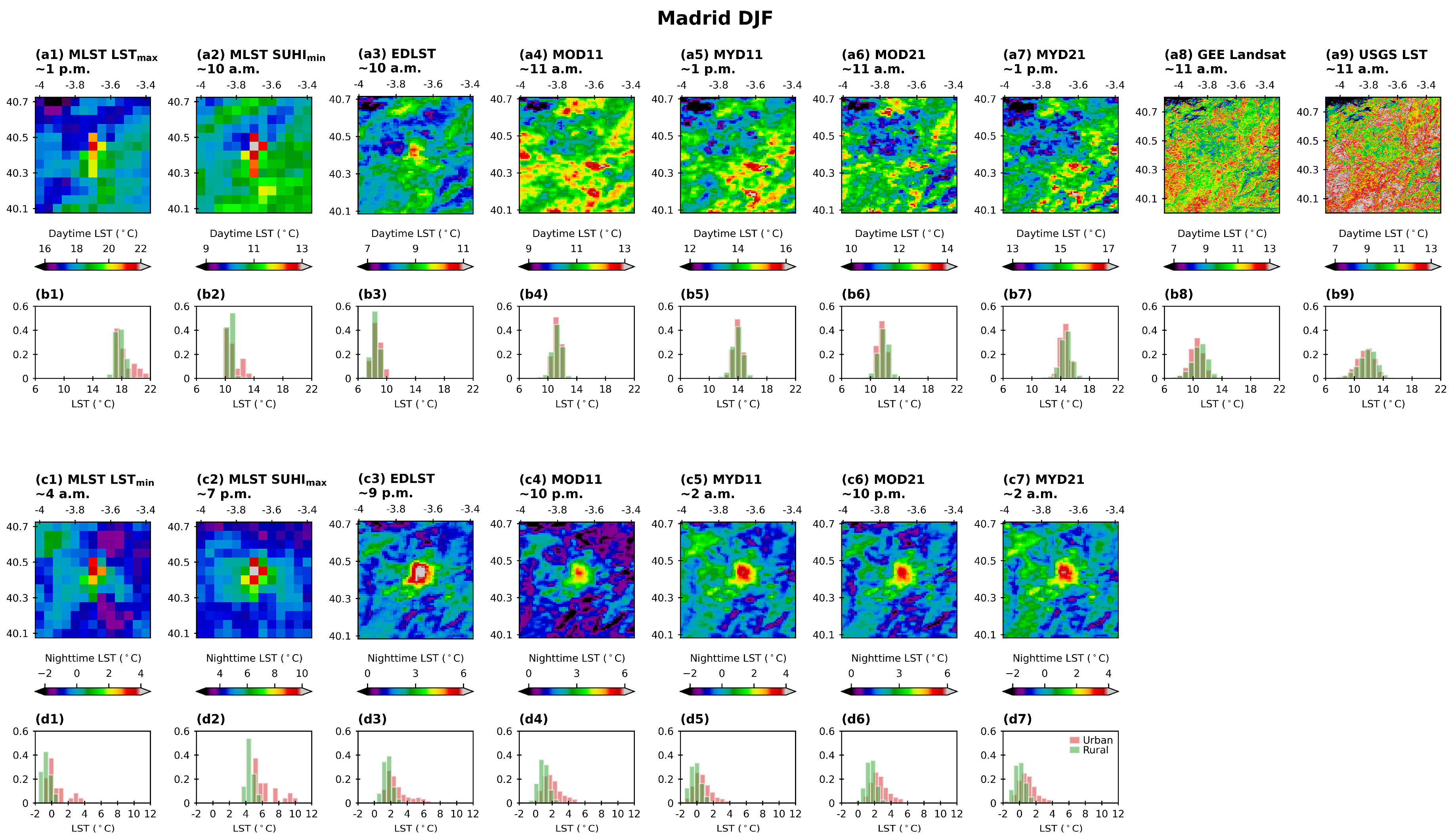
3.2. Spatial Distribution

The spatial patterns of LST at the two regions of interest, as given by the different products in different seasons, are shown in Figure 3, Figure 4, Figure 5 and Figure 6. The respective distribution of LST values within the rural and urban areas is also shown. Note that the hour of observation shown is a rounded mean hour for the respective season and even in the cases where the hour of MLST LSTmin/max and MLST SUHImin/max are the same, LST values may vary as they are not considered at the exact same 15 timesteps. Also, color bars are different for each product to allow a better visualization of the spatial patterns, but histograms show the same LST range.
For Madrid, during daytime (and SUHImin time) in the winter months (Figure 3(a1–a9)), patterns of LST are similar between products, apart from MLST and EDLST where values are increasing from NW to SE directions and with a distinct pattern of higher temperatures in the urban area. For the remaining products, the NW-SE gradient still exists but no evident pattern of higher temperatures associated with the urban area is visible. MLST and EDLST products suggest positive SUHI intensity given the larger difference between the distribution of temperatures for urban and rural areas. Focusing on the histograms (Figure 3(b1–b9)), the highest LSTs, both urban and rural, occur for the MLST LSTmax with values ranging between 16 and 22 °C, followed by the MYD21 product with LSTs ranging between 13 and 17 °C. The lowest LSTs are associated with the EDLST product, ranging between 7 and 10 °C, followed by the Landsat products, both presenting values between 8 and 14 °C. The Landsat products show a wider distribution of LST values in the histograms when compared to the coarser products. This is due to the much higher spatial resolution that allows a more detailed characterization of the surface spatial variability.
During winter nighttime (and SUHImax time) over Madrid (Figure 3(c1–c7)), LST patterns are similar between products, with a higher distinction between urban and rural temperatures, and clear warmer temperatures over the urban area. The spatial pattern of the urban region is more clearly defined in the 1 km products, as expected. The lowest LSTs are associated with the MLST LSTmin ranging from −1 to 4 °C (−2 to 1 °C) for urban (rural) areas followed by the MYD11 and MYD21 products with values of −1 to 2 °C (−1 to 3 °C) for urban (rural) areas. The highest LSTs are associated with MLST SUHImax with urban temperatures ranging from 5 to 10 °C and rural ones from 3 to 6 °C.
During summertime in Madrid, all LST products show a similar signal during daytime (SUHImin; Figure 4(a1–a9,b1–b9)), with slightly cooler urban temperatures when compared to the rural ones. Cooler temperatures are also associated with the regions of the Jarama and Tagus rivers to the SE, more noticeable for the PO-based products, and the mountainous regions in the NW. Again, the highest LSTs are associated with MLST LSTmax, with values of 45 to 50 °C (43 to 52 °C) for urban (rural) regions, followed by both MYD products with temperatures ranging from 44 to 50 °C (40 to 50 °C) in urban (rural) regions for MYD21 and 40 to 48 °C (39 to 48 °C) in urban (rural) regions for the MYD11 product. The lowest LST values are associated with the EDLST and MOD11 products, ranging from 35 to 45 °C. Again, Landsat products show a significantly wider distribution of LSTs resulting from the more detailed spatial representation. During nighttime (SUHImax; Figure 4(a1–a9,b1–b9)), a higher distinction is seen between urban and rural LSTs for all products. The lowest LSTs are associated with MLST LSTmin, ranging between 16 and 21 °C (14 and 18 °C) in urban (rural) areas. The highest LST values are associated with MLST SUHImax, with values ranging from 22 to 27 °C (18 to 21 °C) in urban (rural) areas. The LST distributions are close for the MLST SUHImax and MOD11 product. The distribution of the MOD21 and EDLST products are also similar. These show higher LST values despite being associated with observation times similar to MLST SUHImax and MOD11.
For Paris, during daytime (and SUHImax time) in winter (Figure 5(a1–a9)), there is a general pattern of higher temperatures for the urban areas compared to the rural ones. The spatial patterns are generally consistent across the different products, but the LST contrast between the rural and urban environments is very variable. Despite the higher resolutions, the Landsat products show a less defined urban pattern when compared to the 1 km products, which is also noticeable when analyzing the LST distribution histograms (Figure 5(b1–b9)). The highest temperatures are associated with both MLST products (LSTmin and SUHImin), with values ranging from 9 to 15 °C (7 to 10 °C) in urban (rural) areas. The MLST product also shows higher variability in LST values over the urban area, likely related to the density of urban materials (as seen in Figure 1j). Despite having similar observation times, the MYD11 and MYD21 products show LSTs that are generally lower than the MLST; the MYD11 presents stronger contrasts between urban and rural areas than the MYD21. The lowest values are associated with the EDLST product where urban temperatures range from 3 to 8 °C and rural ones from 3 to 6 °C. All the products with morning overpasses (EDLST, MOD, and Landsat) show LSTs with similar ranges, with the EDLST having slightly lower temperatures in the rural region. During nighttime (SUHImin), a clear distinction between urban and rural temperatures still exists, and patterns are similar between the products. As expected, the lowest temperatures correspond to the MLST LSTmin product, ranging from −1 to 3 °C (−1 to 0 °C) for urban (rural areas). In this case, the highest LST values are seen for the EDLST product ranging between 1 and 6 °C (1 and 3 °C) in urban (rural) regions. The EDLST product also shows the widest spread of urban LST values, indicating a higher sensitivity to the urban density.
During Paris daytime (SUHImax) in summer (Figure 6(a1–a9)), there is also a clear distinction between the urban (higher) and rural (lower) temperatures, with overall similar patterns across all sensors that are more defined as the resolution increases. The highest LST values are associated with MLST LSTmax, ranging between 32 and 43 °C (31 and 36 °C) for urban (rural) areas. The MYD11 and MYD21 products present LST values with similar range, the MYD21 being slightly warmer overall. For the morning overpasses, EDLST and MOD11 show close values of LST but the clusters of warmer LSTs have different locations. The EDLST cluster of warmer LSTs shows better agreement with the MLST product than the other 1 km products, while the MOD11 shows two well-defined clusters in the northern and southern part of the city that are consistent for all MODIS and Landsat products. MOD21 shows a spatial pattern similar to MOD11 but generally with warmer temperatures. The lowest temperatures correspond to the Landsat products ranging between 25 and 40 °C (22 and 34 °C) for GEE Landsat and between 22 and 37 °C (22 and 35 °C) for USGS Landsat. This is likely a result of the time of observation and increased spatial sampling. During nighttime (SUHImin), patterns and clusters of warmer temperatures are more consistent between the products. Again, the lowest temperatures are associated with MLST LSTmin, with temperatures from 13 to 17 °C (11 to 14 °C) for urban (rural) areas. The highest temperatures are associated with MOD21, EDLST, and MLST SUHImin, with values between around 15 and 25 °C (15 and 20 °C) for urban (rural) areas. There is a conspicuous pattern of very warm LSTs (over 30 °C) for the MOD21 product that is not represented in any of the other products. These correspond to urban areas and reach 39 °C (Figure 6(d8)).

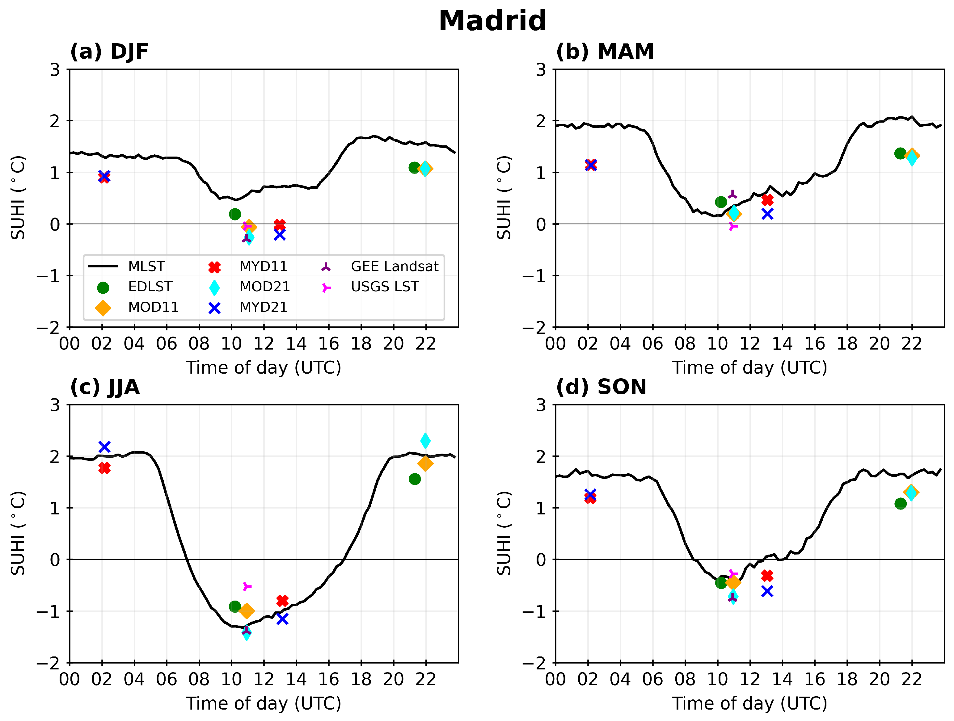
3.3. Diurnal and Seasonal Variability

To understand how the diurnal and seasonal variability is represented by each product, seasonal averages of the SUHI were computed for the day and night and at every 15 min in the case of the MLST. Madrid’s seasonal SUHI diurnal cycle (Figure 7) is characterized by higher and positive intensities during nighttime and lower ones during daytime, reaching negative values (cool island) during summer (JJA) and fall (SON; Figure 7c,d). Based on MLST, the largest SUHI intensities occur during the spring (MAM) months (Figure 7b), reaching values of 2 °C that remain stable during the night hours. The minimum SUHI intensity occurs during summertime (JJA) around noon (Figure 7c), reaching negative values of about −1.2 °C. This is also the season with the highest SUHI diurnal amplitude. The peak of the daytime negative SUHI tends to occur mid-morning, while the maximum of SUHI occurring during the nighttime shows a less defined peak at sunset, and with very stable SUHI values throughout the night. Nighttime SUHI computed based on PO sensors usually displays smaller intensities when compared to the MLST product, with the exception of summer (JJA) months. EDLST SUHI is always lower than MLST during nighttime (time of SUHImax) and slightly higher (lower absolute value) during the daytime of spring and summer (Figure 7b,c), leading overall to reduced SUHI amplitudes. MxD11 and MxD21 present similar SUHI intensities that are usually lower than the MLST SUHI, with the exception of summer months (Figure 7c). For those months, MxD21 (MxD11) tends to have higher (lower) SUHI during the night, and lower (higher) SUHI values during the day, i.e., higher (lower) intensity of the negative daytime SUHI. GEE Landsat SUHI shows similar intensities to the MLST for JJA and MAM, but intensity is lower in DJF and higher during SON. Conversely, USGS LST SUHI intensities are similar to the MSLT in the intermediate seasons (SON and MAM) and are lower for winter (DJF) and summer (JJA).
Regarding the seasonal behavior in Madrid, MLST shows a progressive variation in the nighttime SUHI from around 2 °C in JJA to approximately 1.5 °C in DJF. For the PO products (except the Landsat products), nighttime SUHI is fairly stable at 1 °C during most of the year, increasing to 1.5 °C to 2.3 °C in JJA. The MLST daytime SUHI also shows a smooth variation throughout the year, going from around 0.5 °C in DJF to 0.1 °C in MAM, −1.2 °C in JJA, and −0.4 °C in SON. For the PO satellites, the SUHI seasonal cycle is less pronounced, going from −0.1 to 0.2 °C in DJF, 0 °C to 0.6 °C in MAM, −1.2 °C to −0.5 °C in JJA, and −0.9 to −0.3 °C in SON. Here, the time of observation does not seem to have a significant impact, with morning and afternoon PO showing similar ranges of values.
For the Paris SUHI diurnal cycle (Figure 8), based on the MLST product, the maximum SUHI occurs in springtime (MAM) at noon, reaching 4.5 °C (Figure 8b). Secondary maxima can occur during the nighttime, particularly during summer when nighttime SUHI reaches 3.8 °C. Minima are concentrated during the early hours of both the day and night with the lowest values reaching 1.2 °C during the winter months (Figure 8c). The diurnal amplitude based on PO sensors is highly variable between products, and SUHI values tend to be significantly lower than for MLST. During winter and fall, PO products do not show considerable differences in SUHI intensity between the day and night (Figure 8a,d). The EDLST product has a higher diurnal amplitude during spring and summertime (Figure 8b,c). The MODIS products show similar SUHI values for the same overpass times, with the exception of the nighttime MOD21 SUHI in JJA. The MOD21 nighttime summer SUHI is conspicuously high (Figure 8c) and is not comparable to any of the other products considered. GEE Landsat SUHIs show a high variability, being close to the other PO products during DJF and SON but presenting significantly higher SUHIs in MAM and JJA, reaching values of about 4.5 °C. The USG LST shows the lowest daytime SUHI of all the sensors, only reaching 2.5 °C during MAM/JJA.
Considering the seasonal variation in the SUHI in Paris, again, the MLST shows a smooth transition between seasons, with daytime maximum SUHI values varying from 2.9 °C in DJF, 4.5 °C in MAM, 4.0 °C in JJA, to 3.8 °C in SON. The PO products show a reduced amplitude of the seasonal cycle, with DJF SUHI values of about 0.5 °C to 1.2 °C, MAM values around 2.5 °C to 3.1 °C, JJA values around 2.4 °C to 3.5 °C, and SON values around 0.8 °C to 1.5 °C. The exception is the GEE Landsat that presents the highest seasonal variations, going from 0.8/1.2 °C in DJF/SON to 4.5 °C in MAM/JJA. The nighttime SUHI (or SUHImin) shows lower seasonal variations. Based on the MLST product, the SUHImin varies from about 1.2 °C in DJF, 1.8 °C in MAM, 1.7 °C in JJA, to 1.2 °C in SON. For MODIS and EPS products, nighttime SUHI is around 0.3 °C to 1.1 C during DJF, 1.1 °C to 2.0 °C during MAM, 2.0 °C to 2.6 °C during JJA (excluding MOD21), and 0.8 °C to 1.7 °C during SON.

3.4. Inter-Annual Variability

We further wish to analyze how SUHI inter-annual variability is represented by the different products. For that purpose, correlation coefficients were computed for each pair of SUHI monthly anomalies.
In regards to Madrid during daytime (SUHImin; Figure 9a), the lowest correlations are seen for the GEE Landsat and USGS LST with values ranging from 0.34 to 0.5 and 0.45 to 0.61, respectively. Correlations between MLST SUHI and the remaining products range between 0.76 and 0.8. The highest correlations are seen between the EDLST, MOD11, MYD11, MOD21, and MYD21 products, ranging between 0.89 and 0.97.
During nighttime (SUHImax; Figure 9b), correlations are lower. MLST SUHI presents the weakest correlations, with values ranging between 0.2 and 0.23 and no significant correlation (at a p-value of 0.05) with the MOD21 product. For the EDLST product, all correlations are significant with values of 0.31, 0.59, 0.61, and 0.66 for MOD21, MYD21, MYD11, and MOD11, respectively. MODIS products usually have correlations above 0.6, among themselves, except for the MOD21/MYD11 and MYD21/MOD21 pairs showing correlations of 0.36 and 0.39, respectively.
Regarding Paris during daytime (SUHImax; Figure 10a), USGS LST presents only one significant correlation, with the GEE Landsat product, with a value of 0.37. In turn, GEE Landsat has only three additional significant correlations, with the MYD11, MOD21, and MYD11 products, with values of 0.22 for the first two and 0.27 for the last one. All remaining correlations are significant and higher than the Landsat product ones. The highest correlations correspond to the pairs MYD21/MYD11, MOD21/MOD11, and MYD11/MOD11 with values of 0.82, 0.79, and 0.68, respectively. Correlations for the remaining pairs are within 0.34 and 0.56.
During nighttime (SUHImin; Figure 10b) for Paris, the pair MOD11/MLST SUHI has no significant correlation. The lowest correlations correspond to the MOD21/EDLST, MOD21/MYD11, MYD21/MOD21, MOD11/MLST SUHI, and MYD21/MLST SUHI pairs of products, with values of 0.22, 0.29, 0.32, 0.43, and 0.45, respectively. Correlations between 0.52 and 0.58 are associated with the EDLST/MLST SUHI, MYD11/MLST SUHI, MYD11/MOD11, MYD21/EDLST, MYD11/EDLST, MYD21/MOD11, MOD11/EDLST, and MOD21/MOD11. The highest correlation is associated with the MYD21/MYD11 pairs of products, reaching a value of 0.83.

3.5. Product Inter-Comparison

To further investigate the differences in SUHI as given by each LST product, we perform an inter-comparison between the LST products. For that purpose, we reproject all products onto the MLST grid (the coarser grid) and then compute the mean of monthly differences between the sensors for Madrid and Paris (Table 2 and Table 3, respectively). For differences between MLST and the other products, we use the MLST time of observation closest to the PO time. For comparisons between PO products, we aggregate them in groups with similar overpass times, i.e., in morning and afternoon overpass. Although differences in LST may be significant due to differences in observation time, this analysis may provide useful information to understand the observed differences of the SUHI. The respective maps of LST differences between products and scatterplots of LSTs are also available in the Supplementary Materials.
For the Madrid region (Table 2), the highest LST differences occur during daytime (regardless of the sensors considered). When comparing MLST with PO products at the same hours of observation, the bias is usually positive, indicating that the MLST tends to show higher LSTs than all the remaining products, particularly during the daytime. The largest differences between MLST and remaining products are associated with MYD11, GEE Landsat, and MOD11 with values of 3.52, 2.99, and 2.65 °C, respectively. The maps of LST differences (Figures S1–S3 of Supplementary Materials) also indicate that differences with respect to MLST tend to be larger over the urban area. The EDLST shows negative mean differences with respect to all the remaining PO products during the daytime, with the largest differences, of −3.1 and −3.05 °C, occurring for the USGS and MOD21 products, respectively. When compared to MODIS, EDLST is expected to have lower daytime LSTs given the earlier overpass time, but the time of observation for the Landsat is similar. The nighttime differences between EDLST and MODIS products are positive, being largest for the MOD11 with a value of 1.29 °C. Differences between the MODIS products are also significant, particularly during daytime. The MxD11 product shows on average lower temperatures than the MxD21 product, with mean difference values of −1.12 °C (−0.97 °C) and −1.16 °C (−0.58 °C) during the day (night) for the morning (MODx1) and afternoon (MYDx1) times, respectively. During daytime, the smallest difference between sensors is associated with MOD21/USGS LST and MOD11/GEE Landsat with values of −0.17 and −0.39 °C, respectively. However, differences in the observation time of MODIS/Terra and the Landsat are expected to result in larger LST differences, with the Landsat LSTs being lower, and, therefore, LST differences should be positive. Despite the overall low mean differences of the Landsat products, maps of the differences show a very high spatial heterogeneity with biases varying from approximately −3 to 3 °C at the pixel level for both the MOD21/USGS LST and MOD11/GEE Landsat pairs (see Supplementary Materials).
Over the Paris region (Table 3), larger differences between products are also seen during the daytime. The MLST product also generally presents higher LST values than the remaining products during the day, the highest values of mean differences being 3.55 °C, 3.36 °C, 3.30 °C, and 2.93 °C when compared to USGS LST, MYD11, MOD11, and GEE Landsat, respectively. Like in the case of Madrid, differences tend to be larger over the urban area (Figures S4–S6 of the Supplementary Materials). EDLST tends to be cooler than the other PO products during the day and warmer during the night, the largest differences being found when comparing with MOD21 with a mean value of −2.65 °C. Again, differences between the MODIS products are consistent with those found for Madrid, the MxD11 showing overall lower LSTs than the MxD21, with mean differences of −1.42 °C (−1.03 °C) and −1.30 °C (−0.46 °C) for the day (night) when comparing the morning (MODx1) and afternoon (MYDx1) overpasses, respectively. The smallest difference is seen during nighttime, for the MLST/MOD11 products. The lowest differences were found between GEE Landsat and MOD11 and between the two Landsat LSTs, with values of 0.07 °C and −0.03 °C, respectively. Like in the case of Madrid, the spatial variability in the differences is very high for the Landsat products and pixel level biases range from −6 to 6 °C (Figures S5 and S7 of the Supplementary Materials).

4. Discussion

The availability of remote sensing data is dependent on the platform’s type of orbit, which is the most influential factor in dictating the maximum temporal and spatial resolution that sensors can achieve. The difference in temperature between urban areas and their surroundings is more easily evaluated based on remote sensing sources than in situ data. While the former is of outmost importance in calibrating and validating remote sensing observations, its use in understanding urban heat islands is highly specific to the region where its located. Remote sensing observations enable urban thermal studies from a local city scale to a global one. One of the greatest disadvantages of remote sensing observations is the trade-off between temporal and spatial resolution. Sensors onboard low-orbiting platforms (polar orbiting) can achieve higher spatial resolutions, of the order of one kilometer to tenths of meters, which is of substantial importance when examining LST in highly heterogeneous areas such as cities and their surroundings. Conversely, sensors onboard high-orbiting platforms (such as geostationary orbits) have a much higher observation rate. This allows a characterization of the diurnal cycle while also dampening the effect of clouds in thermal-derived observations [81]. Another limitation of remote sensing observations is the inherent 2D characterization of the surface temperature that restrains SUHI depiction to a “bird’s eye view”, ignoring the distinct contribution of 3D walls, rooftops, and “urban canyons” [81].
Although LST products derived from sensors onboard different platforms are used in urban climate studies [20], most users are not aware of the potential impact of the choice of LST product on their SUHI analysis. In this work, we aim to provide some insights into the differences between LST products in urban regions and their impact in SUHI estimation, enabling a more informed decision by users when selecting an LST product for SUHI studies. For that purpose, four polar orbiting and one geostationary platform were considered, also including different retrieval algorithms for the same sensor. This allows for investigating the impact of not only temporal and spatial resolution on SUHI computations, but also potential biases between the products due to algorithm formulation.
Two cities were analyzed: Madrid and Paris. These cities were selected because they have very distinct behaviors of the SUHI. As Madrid is a city embedded in a seasonally dry climate with little rainfall during the coldest and hottest months (DJF and JJA), the rural area is composed by barren land and dry vegetation during these seasons. In particular, during summer, the irrigation of urban parks and gardens increases evapotranspiration in the urban area compared to the dry rural one. This leads to evaporative cooling in the city due to a decrease in sensible heat and an increase in latent heat. For the rural areas, drier areas’ water availability is lower, limiting the evaporative cooling [90]. These characteristics translate into maximum SUHI intensities occurring during nighttime and lower ones during daytime. In the summer months (JJA), SUHI can reach negative values, i.e., an urban cool island [35,78,79,80,81,82,83]. The city of Paris is embedded in a wetter climate where evapotranspiration is in phase with radiation, leading to cooling of natural (rural) surfaces. Such cities are often characterized by positive SUHI values all year round, with maxima during daytime and seasonally in summertime [35,44,78,80,81,82,83].
We started by analyzing the distribution of the overpass time amongst the products. It is shown that the observation time associated with PO satellites does not necessarily coincide with the time of the maximum and minimum of either LST or SUHI, as given by the GEO satellite (Figure 2). The hour of maximum LST is generally associated with the hour of maximum incoming radiation, while the minimum of LST occurs close to sunrise when the maximum time extent without solar radiation is achieved. Therefore, it is expected that the time of the LST maximum and minimum will vary throughout the year. For the hours of minimum and maximum SUHI intensity, the variability in time is quite large. This is due to SUHI values remaining constant along part of the day, resulting in the minima/maxima hours not being as well defined (see Figure 7 and Figure 8). Also, in the case of Paris, a secondary maximum and minimum is developed (Figure 8c) along the day, impacting the hour considered for the limits of diurnal SUHI. This analysis suggests that, in the case of Madrid, POs with afternoon overpass are closer to the daytime SUHI minimum, while the morning overpass POs are closer to the hour of the nighttime SUHI maximum. In the case of Paris, the SUHI maximum might be well represented by POs with afternoon overpass, but the hour of the SUHI minimum is not well captured by any of the POs.
We then investigated the spatial patters of LST as given by the different products (Figure 3, Figure 4, Figure 5 and Figure 6). As expected, products with higher spatial resolution can provide more detailed maps of LST. For cities of smaller sizes such as Madrid, the coarser-resolution MLST products are likely not able to provide much detail into the spatial variability within the city. We found that, despite the difference in resolution, the major patterns like the urban area or rivers are generally consistent between products. However, amplitudes of LSTs are very different, and, in particular, contrasts between the urban and rural environment are significantly different, which ultimately will result in different SUHI values. Also, we found that, despite the higher resolution, PO products do not necessarily show higher contrasts between urban and rural pixels. We also found that in the city of Paris, the daytime LST values as given by the POs show maximums within the city at different locations. This is particularly relevant for studies where the SUHI is analyzed at the more local level (e.g., at the neighborhood level). Our results suggest that depending on the chosen product, such an analysis may yield very different results. These differences in the LST patterns may be related to differences in the prescribed/retrieved emissivity that is expected to show strong variations due to the high heterogeneity of urban regions. A closer inspection of the products’ emissivities suggests that emissivity contrasts are significantly lower for the MxD21 products when compared to the MLST, EDLST, and MxD11, also being with a reduced seasonality associated with vegetation cover. A reduced seasonality was also found in the MxD11 compared to the MLDT and EDLST. There are also some conspicuously high LST values (over 30 °C) for the MOD21 product in Paris (Figure 6). These may be related to errors in the retrievals by the TES algorithm and seem to be associated with abnormally low emissivity values.
We then proceed to compare the temporal variability in the SUHI as given by each LST product, namely at the diurnal, seasonal, and inter-annual level. Our analysis indicates that there are significant differences in the amplitude of the diurnal and seasonal cycles of SUHI as given by the different products, even when considering close observation times (Figure 7 and Figure 8). As such, any analysis on the diurnal and seasonal variations in SUHI may be impacted by the choice of LST product. Differences in the diurnal amplitudes could be related to the time of observation or temperature-dependent biases in the algorithms. The differences in seasonality may be related to different representations of emissivity seasonality, as well as different accuracies of the retrieval algorithms when performing the atmospheric correction (since atmospheric conditions also show a strong seasonality).
To access the consistency in inter-annual variability in the SUHI for the different products, we computed the correlations between monthly values of SUHI. In the city of Madrid during the daytime (Figure 9a), significant positive correlations were found between all pairs of products with relatively high values (above 0.89), with the exception of the MLST (with values of 0.76–0.80) and the Landsat (with values between 0.34 and 0.61) products. During the nighttime (Figure 9b), the MLST product also shows the smallest correlations with the remaining products, with values within 0.20–0.23. Correlations between most of the PO products are also lower than those found for daytime, with values ranging from 0.31 to 0.68. The highest correlations are seen for the pairs of products belonging to the same sensor, i.e., MxD11/MxD21 (with the exception of the MOD21/MOD11 nighttime value). In Paris (Figure 10), correlations are also low or non-significant for the GEE Landsat and USGS products. Correlations for most pairs of products are also relatively low, with values around 0.3–0.6. As in the case of Madrid, the highest correlations are also obtained for the MxD11/MxD21 pairs of products. During nighttime (Figure 10b), the MOD21 shows the lowest correlations, with an exception for MOD21/MOD11, which is likely due to the conspicuous patterns found in the LSTs.
The relatively lower correlations of the MLST product may be due to the variability in the hour of observation, as the MLST SUHI minimum/maximum may occur at different times of day, depending on the seasonality of the SUHI diurnal cycle. The low correlation values of the Landsat products are likely associated with the low observation sampling in each month, which results in stronger inter-annual variability since only a few days are sampled. Considering that, for Madrid, the highest intensities of the SUHI occur during the nighttime, these results suggest that there is low consistency in the inter-annual variability in the SUHI as provided by each product. The higher correlations of the MODI products suggests a better consistency regardless of the algorithm used to compute LST, and likely the observation time is the major factor influencing the obtained correlations.
Finally, an inter-comparison of the LSTs was performed to assess the biases between products. Results suggest that significant biases exist between the different LST products over urban regions, particularly during the daytime. The MLST is consistently warmer than all other products, with daytime biases ranging from 1.41 to 3.55 °C and nighttime biases ranging from −1.03 to 0.02 °C. In the case of the MLST, comparisons are performed at matching observation times and therefore differences can only be attributed to differences in the retrieval methodology or sensor calibration. The EDLST tends to be cooler than the other POs during the day and warmer during the night, showing daytime biases in the range of −3.10 to −0.50 and nighttime biases in the range of 0.09 to 1.29 °C. These differences are consistent with differences in the observation time in the case of the MODIS but not in the case of the Landsat. When comparing the MODIS products, MxD11 LSTs are generally cooler than MxD21, with biases of −1.12 to −1.42 °C for daytime and −0.46 to −1.03 °C for nighttime. Since these products are derived from the same sensor, differences can only be attributed to the different retrieval methodologies. Regarding the Landsat products, biases against other products and even between the two Landsat products are highly variable. We also found a high spatial variability in the biases. Although all products report product uncertainties of about 2 °C, validation exercises rarely encompass urban environments and, therefore, may not be representative of such environments. In situ measurements of LST for urban areas are not readily available and are likely not representative of the satellite scale due to the high spatial heterogeneity. Therefore, this study is not able to indicate which LST product is more accurate in urban areas.
All the analyses presented in this study were carried out using monthly averages of the LST. On the one hand, this allows a more accurate identification of the LST and SUHI maximum and minimum, since cloud presence at the time of these minimum/maximum values may lead to the selection of the wrong time slot for a specific day. On the other hand, it allows our investigation to be more focused on biases between the products since day-to-day variability is expected to be high due to the algorithms’ uncertainties. We are aware that this may result in larger discrepancies in the case of the Landsat products due to their significantly lower frequency of observations (~16 days). Indeed, the mean difference between the Landsat and other products shows high spatial variability that is likely a result of discrepancies in the days considered when using the monthly averages. However, it is also worth showing the impact of using a sensor with such low observational frequency when analyzing SUHI intra- and inter-annual variability.
The definition of both urban/rural regions and SUHI computation can also be a source in variability when comparing different studies [91]. Considering that most SUHI studies are focused on relatively stable and big cities [9], land cover can be considered as static, meaning that the selection of urban and rural pixels can be considered as nearly unaffected. This is not the case for developing cities where the size of the city, construction materials, and type of rural land cover may significantly change, emphasizing the need for the better understanding of LST variations per land cover. This is particularly important considering the distinction between urban and rural areas largely depending on the spatial resolution of the data, with mixed pixels being associated with a unique land cover type even though they are not representative of it [10].
The products mentioned rely on thermal infrared observations, which are not available in cloudy conditions [21,47]. Most SUHI studies use information in this part of the electromagnetic spectrum, meaning that results are only representative of clear sky conditions [92]. Lastly, it is noteworthy that all LST products have an associated uncertainty that can reach values of 3–4 °C, influenced by atmospheric and surface conditions [47,54]. Consequently, it may be the case that SUHI intensities may be of the same order of magnitude as the LST uncertainties. In the case of the present study, as the spatial scale is relatively small, it is expected that uncertainties for urban and rural areas will be highly correlated, reducing its propagation to SUHI intensities [93].

5. Conclusions

When describing the climate of a certain region, air temperature is essential. Usually, this variable is known for a broad time range and relatively small timesteps, allowing the characterization of the diurnal temperature cycle. As these data are sourced from in situ sensors, satellite remote sensing has been largely applied in characterizing urban climate, taking advantage of its global coverage. The drawback of these datasets is the temporal–spatial resolution compromise. Due to satellite orbits, datasets have either good spatial or good temporal resolution, with SUHI studies usually making use of sensors with higher spatial resolution given the small scale of the urban regions. Moreover, LST as obtained from remote sensing sensors is an indirect measurement of temperature, relying on retrieval algorithms whose quality impacts the uncertainty of the LST estimates.
The present work analyzed land surface temperature from several polar orbiting satellites and one geostationary platform. The aim was to understand if SUHIs attained based on the same method but from different sensors are compatible, as these datasets are largely used in the literature.
Results show that caution must be taken when characterizing SUHI based on a few observations per day, as these may not fully characterize the range of intensities. This can translate into different SUHI intensities or signals (positive/negative). Also, as cities and their surroundings are highly heterogeneous surfaces, low-spatial-resolution datasets may dampen the spatial patterns. Analyses of the diurnal, seasonal, and inter-annual variability in the SUHI also suggest low consistency on the variability as given by each product. Therefore, studies focusing on the study of the SUHI based on a single product may be significantly affected by the choice of product. We also found significant biases between the products even when considering the same resolution and time of observation. The validation of LST products over urban areas is very difficult due to the high heterogeneity, and therefore care must be taken when basing SUHI studies on a single LST product. Moreover, the low sampling rate joined with observations not matching the hours of extremes for either LST or SUHI, and pixel sizes much larger than surface heterogeneity may lead to discrepancies between SUHI results, consequently making it difficult to compare studies, even when representing the same climate and degree of urbanization.

Supplementary Materials

The following supporting information can be downloaded at: https://www.mdpi.com/article/10.3390/rs16203765/s1, Figure S1: Madrid mean LST differences between products with similar daytime times of observation, namely for morning overpasses (MLST was taken at the time of observation of the sensor it is compared with) and respective scatterplots of the LSTs; Figure S2: As Figure S1 but for the afternoon overpasses; Figure S3: As Figure S1 but for all nighttime overpasses; Figure S4: As Figure S1 but for Paris; Figure S5: As Figure S2 but for Paris; Figure S6: As Figure S3 but for Paris.

Author Contributions

Conceptualization, A.H. and S.L.E.; methodology, A.H. and S.L.E.; formal analysis, A.H. and S.L.E.; writing—original draft preparation, A.H.; writing—review and editing, S.L.E.; visualization, A.H.; supervision, S.L.E. and C.C.D. All authors have read and agreed to the published version of the manuscript.

Funding

This research was funded by the Portuguese Fundação para a Ciência e a Tecnologia (FCT) through PhD grant 2020.08063.BD, and by the FCT I.P./MCTES through national funds (PIDDAC)—UIDB/50019/2020-IDL.

Data Availability Statement

The original data presented in the study are openly available.

Conflicts of Interest

The authors declare no conflicts of interest.

References

  1. Torrance, K.; Shun, J. Time-varying energy consumption as a factor in urban climate. Atmos. Environ. 1976, 10, 329–337. [Google Scholar] [CrossRef]
  2. Landsberg, H. The Urban Climate, 1st ed.; Academic Press: Cambridge, MA, USA, 1981; Volume 28, p. 275. Available online: https://www.elsevier.com/books/the-urban-climate/landsberg/978-0-12-435960-4 (accessed on 29 July 2024).
  3. Wilmers, F. Effects of vegetation on urban climate and buildings. Energy Build. 1990, 15, 507–514. [Google Scholar] [CrossRef]
  4. Souch, C.; Grimmond, S. Applied climatology: Urban climate. Prog. Phys. Geogr. 2006, 30, 270–279. [Google Scholar] [CrossRef]
  5. Oke, T.R.; Mills, G.; Christen, A.; Voogt, J. Urban Climates; Cambridge University Press: Cambridge, UK, 2017; pp. 1–525. [Google Scholar] [CrossRef]
  6. Ningrum, W. Urban Heat Island towards Urban Climate. IOP Conf. Ser. Earth Environ. Sci. 2018, 118, 012048. [Google Scholar] [CrossRef]
  7. Lemoine-Rodríguez, R.; Inostroza, L.; Zepp, H. Does urban climate follow urban form? Analysing intraurban LST trajectories versus urban form trends in 3 cities with different background climates. Sci. Total. Environ. 2022, 830, 154570. [Google Scholar] [CrossRef]
  8. Hu, M.; Li, X.; Xu, Y.; Huang, Z.; Chen, C.; Chen, J.; Du, H. Remote sensing monitoring of the spatiotemporal dynamics of urban forest phenology and its response to climate and urbanization. Urban Clim. 2024, 53, 101810. [Google Scholar] [CrossRef]
  9. Zhou, D.; Xiao, J.; Bonafoni, S.; Berger, C.; Deilami, K.; Zhou, Y.; Frolking, S.; Yao, R.; Qiao, Z.; Sobrino, J.A. Satellite Remote Sensing of Surface Urban Heat Islands: Progress, Challenges, and Perspectives. Remote Sens. 2019, 11, 48. [Google Scholar] [CrossRef]
  10. Shi, H.; Xian, G.; Auch, R.; Gallo, K.; Zhou, Q. Urban Heat Island and Its Regional Impacts Using Remotely Sensed Thermal Data—A Review of Recent Developments and Methodology. Land 2021, 10, 867. [Google Scholar] [CrossRef]
  11. Nations, U. Revision of World Urbanization Prospects|United Nations, (n.d.). 2018. Available online: https://www.un.org/en/desa/2018-revision-world-urbanization-prospects (accessed on 29 July 2024).
  12. Oke, T.R. The energetic basis of the urban heat island. Q. J. R. Meteorol. Soc. 1982, 108, 1–24. [Google Scholar] [CrossRef]
  13. Basu, R. High ambient temperature and mortality: A review of epidemiologic studies from 2001 to 2008. Environ. Health Glob. Access Sci. Source 2009, 8, 40. [Google Scholar] [CrossRef]
  14. D’Ippoliti, D.; Michelozzi, P.; Marino, C.; De’Donato, F.; Menne, B.; Katsouyanni, K.; Kirchmayer, U.; Analitis, A.; Medina-Ramón, M.; Paldy, A.; et al. The impact of heat waves on mortality in 9 European cities: Results from the EuroHEAT project. Environ. Health 2010, 9, 37. [Google Scholar] [CrossRef] [PubMed]
  15. Heaviside, C.; Vardoulakis, S.; Cai, X.-M. Attribution of mortality to the urban heat island during heatwaves in the West Midlands, UK. Environ. Health 2016, 15, 49–59. [Google Scholar] [CrossRef] [PubMed]
  16. Guo, Y.; Gasparrini, A.; Armstrong, B.G.; Tawatsupa, B.; Tobias, A.; Lavigne, E.; De Sousa Zanotti Stagliorio Coelho, M.; Pan, X.; Kim, H.; Hashizume, M.; et al. Heat Wave and Mortality: A Multicountry, Multicommunity Study. Environ. Health Perspect. 2017, 125, 087006. [Google Scholar] [CrossRef]
  17. Bastarrika, A.; Chuvieco, E.; Martín, M.P. Mapping burned areas from Landsat TM/ETM+ data with a two-phase algorithm: Balancing omission and commission errors. Remote Sens. Environ. 2011, 115, 1003–1012. [Google Scholar] [CrossRef]
  18. Guo, Y.; Gasparrini, A.; Armstrong, B.G.; Tawatsupa, B.; Tobias, A.; Lavigne, E.; De, M.; Zanotti, S.; Coelho, S.; Pan, X.; et al. Urban Air Pollution, Urban Heat Island and Human Health: A Review of the Literature. Sustainability 2022, 14, 9234. [Google Scholar] [CrossRef]
  19. Tomlinson, C.J.; Chapman, L.; Thornes, J.E.; Baker, C. Remote sensing land surface temperature for meteorology and climatology: A review. Meteorol. Appl. 2011, 18, 296–306. [Google Scholar] [CrossRef]
  20. de Almeida, C.R.; Teodoro, A.C.; Gonçalves, A. Study of the Urban Heat Island (UHI) Using Remote Sensing Data/Techniques: A Systematic Review. Environments 2021, 8, 105. [Google Scholar] [CrossRef]
  21. Voogt, J.A.; Oke, T.R. Thermal remote sensing of urban climates. Remote Sens. Environ. 2003, 86, 370–384. [Google Scholar] [CrossRef]
  22. Nguyen, L.H.; Henebry, G.M.; Bechtel, B.; Keramitsoglou, I.; Kotthaus, S.; Voogt, J.A.; Zakšek, K.; Li, Z.; Thenkabail, P.S. Urban Heat Islands as Viewed by Microwave Radiometers and Thermal Time Indices. Remote Sens. 2016, 8, 831. [Google Scholar] [CrossRef]
  23. Duan, S.-B.; Han, X.-J.; Huang, C.; Li, Z.-L.; Wu, H.; Qian, Y.; Gao, M.; Leng, P. Land Surface Temperature Retrieval from Passive Microwave Satellite Observations: State-of-the-Art and Future Directions. Remote Sens. 2020, 12, 2573. [Google Scholar] [CrossRef]
  24. Hamilton, S.L.; Bell, T.W.; Watson, J.R.; Grorud-Colvert, K.A.; Menge, B.A. Remote sensing: Generation of long-term kelp bed data sets for evaluation of impacts of climatic variation. Ecology 2020, 101, e03031. [Google Scholar] [CrossRef] [PubMed]
  25. Cotlier, G.I.; Jimenez, J.C. The Extreme Heat Wave over Western North America in 2021: An Assessment by Means of Land Surface Temperature. Remote Sens. 2022, 14, 561. [Google Scholar] [CrossRef]
  26. Wu, X.; Liu, Q.; Huang, C.; Li, H. Mapping Heat-Health Vulnerability Based on Remote Sensing: A Case Study in Karachi. Remote Sens. 2022, 14, 1590. [Google Scholar] [CrossRef]
  27. Wang, X. Application of Remote Sensing Technology in Different Natural Disasters. Highlights Sci. Eng. Technol. 2023, 44, 390–400. [Google Scholar] [CrossRef]
  28. Duguay-Tetzlaff, A.; Bento, V.A.; Göttsche, F.M.; Stöckli, R.; Martins, J.P.A.; Trigo, I.; Olesen, F.; Bojanowski, J.S.; Da Camara, C.; Kunz, H. Meteosat Land Surface Temperature Climate Data Record: Achievable Accuracy and Potential Uncertainties. Remote Sens. 2015, 7, 13139–13156. [Google Scholar] [CrossRef]
  29. Shang, H.; Letu, H.; Nakajima, T.Y.; Wang, Z.; Ma, R.; Wang, T.; Lei, Y.; Ji, D.; Li, S.; Shi, J. Diurnal cycle and seasonal variation of cloud cover over the Tibetan Plateau as determined from Himawari-8 new-generation geostationary satellite data. Sci. Rep. 2018, 8, 1105. [Google Scholar] [CrossRef] [PubMed]
  30. Lu, J.; Jia, L.; Zheng, C.; Tang, R.; Jiang, Y. A Scheme to Estimate Diurnal Cycle of Evapotranspiration from Geostationary Meteorological Satellite Observations. Water 2020, 12, 2369. [Google Scholar] [CrossRef]
  31. Penn, E.; Holloway, T. Evaluating current satellite capability to observe diurnal change in nitrogen oxides in preparation for geostationary satellite missions. Environ. Res. Lett. 2020, 15, 034038. [Google Scholar] [CrossRef]
  32. Wu, J.; Goes, J.I.; Gomes, H.D.R.; Lee, Z.; Noh, J.-H.; Wei, J.; Shang, Z.; Salisbury, J.; Mannino, A.; Kim, W.; et al. Estimates of diurnal and daily net primary productivity using the Geostationary Ocean Color Imager (GOCI) data. Remote Sens. Environ. 2022, 280, 113183. [Google Scholar] [CrossRef]
  33. Ng, E.; Ren, C. The Urban Climatic Map: A Methodology for Sustainable Urban Planning; Routledge: Oxfordshire, UK, 2015; p. 474. [Google Scholar]
  34. Deilami, K.; Kamruzzaman, M.; Liu, Y. Urban heat island effect: A systematic review of spatio-temporal factors, data, methods, and mitigation measures. Int. J. Appl. Earth Obs. Geoinf. 2018, 67, 30–42. [Google Scholar] [CrossRef]
  35. Manoli, G.; Fatichi, S.; Bou-Zeid, E.; Katul, G.G. Seasonal hysteresis of surface urban heat islands. Proc. Natl. Acad. Sci. USA 2020, 117, 7082–7089. [Google Scholar] [CrossRef] [PubMed]
  36. Nichol, J.E.; To, P.H. Temporal characteristics of thermal satellite images for urban heat stress and heat island mapping. ISPRS J. Photogramm. Remote Sens. 2012, 74, 153–162. [Google Scholar] [CrossRef]
  37. Xiao, J.; Fisher, J.B.; Hashimoto, H.; Ichii, K.; Parazoo, N.C. Emerging satellite observations for diurnal cycling of ecosystem processes. Nat. Plants 2021, 7, 877–887. [Google Scholar] [CrossRef] [PubMed]
  38. Fabrizi, R.; De Santis, A.; Gomez, A. Satellite and Ground-Based Sensors for the Urban Heat Island Analysis in the City of Madrid. (n.d.). Available online: http://gestiona.madrid.org/ (accessed on 29 July 2024).
  39. Zhou, J.; Chen, Y.; Zhang, X.; Zhan, W. Modelling the diurnal variations of urban heat islands with multi-source satellite data. Int. J. Remote Sens. 2013, 34, 7568–7588. [Google Scholar] [CrossRef]
  40. Choi, Y.Y.; Suh, M.S.; Park, K.H. Assessment of Surface Urban Heat Islands over Three Megacities in East Asia Using Land Surface Temperature Data Retrieved from COMS. Remote Sens. 2014, 6, 5852–5867. [Google Scholar] [CrossRef]
  41. Chang, Y.; Xiao, J.; Li, X.; Frolking, S.; Zhou, D.; Schneider, A.; Weng, Q.; Yu, P.; Wang, X.; Li, X.; et al. Exploring diurnal cycles of surface urban heat island intensity in Boston with land surface temperature data derived from GOES-R geostationary satellites. Sci. Total. Environ. 2021, 763, 144224. [Google Scholar] [CrossRef]
  42. Chang, Y.; Xiao, J.; Li, X.; Zhou, D.; Wu, Y. Combining GOES-R and ECOSTRESS land surface temperature data to investigate diurnal variations of surface urban heat island. Sci. Total. Environ. 2022, 823, 153652. [Google Scholar] [CrossRef] [PubMed]
  43. Hurduc, A.; Ermida, S.L.; Trigo, I.F.; DaCamara, C.C. Importance of temporal dimension and rural land cover when computing surface urban Heat Island intensity. Urban Clim. 2024, 56, 102013. [Google Scholar] [CrossRef]
  44. Zakšek, K.; Oštir, K. Downscaling land surface temperature for urban heat island diurnal cycle analysis. Remote Sens. Environ. 2012, 117, 114–124. [Google Scholar] [CrossRef]
  45. Keramitsoglou, I.; Kiranoudis, C.T.; Weng, Q. Downscaling Geostationary Land Surface Temperature Imagery for Urban Analysis. IEEE Geosci. Remote Sens. Lett. 2013, 10, 1253–1257. [Google Scholar] [CrossRef]
  46. Bah, A.R.; Norouzi, H.; Prakash, S.; Blake, R.; Khanbilvardi, R.; Rosenzweig, C. Spatial Downscaling of GOES-R Land Surface Temperature over Urban Regions: A Case Study for New York City. Atmosphere 2022, 13, 332. [Google Scholar] [CrossRef]
  47. Li, Z.-L.; Tang, B.-H.; Wu, H.; Ren, H.; Yan, G.; Wan, Z.; Trigo, I.F.; Sobrino, J.A. Satellite-derived land surface temperature: Current status and perspectives. Remote Sens. Environ. 2013, 131, 14–37. [Google Scholar] [CrossRef]
  48. Li, Z.; Wu, H.; Duan, S.; Zhao, W.; Ren, H.; Liu, X.; Leng, P.; Tang, R.; Ye, X.; Zhu, J.; et al. Satellite Remote Sensing of Global Land Surface Temperature: Definition, Methods, Products, and Applications. Rev. Geophys. 2023, 61. [Google Scholar] [CrossRef]
  49. Becker, F.; Li, Z.L. Towards a local split window method over land surfaces. Int. J. Remote Sens. 1990, 11, 369–393. [Google Scholar] [CrossRef]
  50. Wan, Z.; Dozier, J. A generalized split-window algorithm for retrieving land-surface temperature from space. IEEE Trans. Geosci. Remote Sens. 1996, 34, 892–905. [Google Scholar] [CrossRef]
  51. Trigo, I.F.; Monteiro, I.T.; Olesen, F.; Kabsch, E. An assessment of remotely sensed land surface temperature. J. Geophys. Res. Atmos. 2008, 113, D17108. [Google Scholar] [CrossRef]
  52. Wan, Z. New refinements and validation of the collection-6 MODIS land-surface temperature/emissivity product. Remote Sens. Environ. 2014, 140, 36–45. [Google Scholar] [CrossRef]
  53. Becker, F. The impact of spectral emissivity on the measurement of land surface temperature from a satellite. Int. J. Remote Sens. 1987, 8, 1509–1522. [Google Scholar] [CrossRef]
  54. Freitas, S.C.; Trigo, I.F.; Bioucas-Dias, J.M.; Gottsche, F.-M. Quantifying the Uncertainty of Land Surface Temperature Retrievals From SEVIRI/Meteosat. IEEE Trans. Geosci. Remote Sens. 2010, 48, 523–534. [Google Scholar] [CrossRef]
  55. Ghent, D.; Veal, K.; Trent, T.; Dodd, E.; Sembhi, H.; Remedios, J. A New Approach to Defining Uncertainties for MODIS Land Surface Temperature. Remote Sens. 2019, 11, 1021. [Google Scholar] [CrossRef]
  56. Artis, D.A.; Carnahan, W.H. Survey of emissivity variability in thermography of urban areas. Remote Sens. Environ. 1982, 12, 313–329. [Google Scholar] [CrossRef]
  57. Mohamed, A.A.; Odindi, J.; Mutanga, O. Land surface temperature and emissivity estimation for Urban Heat Island assessment using medium- and low-resolution space-borne sensors: A review. Geocarto Int. 2017, 32, 455–470. [Google Scholar] [CrossRef]
  58. Chakraborty, T.; Lee, X.; Ermida, S.; Zhan, W. On the land emissivity assumption and Landsat-derived surface urban heat islands: A global analysis. Remote Sens. Environ. 2021, 265, 112682. [Google Scholar] [CrossRef]
  59. Chen, F.; Yang, S.; Su, Z.; Wang, K. Effect of emissivity uncertainty on surface temperature retrieval over urban areas: Investigations based on spectral libraries. ISPRS J. Photogramm. Remote Sens. 2016, 114, 53–65. [Google Scholar] [CrossRef]
  60. Gillespie, A.; Rokugawa, S.; Matsunaga, T.; Cothern, J.S.; Hook, S.J.; Kahle, A.B. A temperature and emissivity separation algorithm for advanced spaceborne thermal emission and reflection radiometer (ASTER) images. IEEE Trans. Geosci. Remote Sens. 1998, 36, 1113–1126. [Google Scholar] [CrossRef]
  61. Hulley, G.C.; Hook, S.J. Generating consistent land surface temperature and emissivity products between ASTER and MODIS data for earth science research. IEEE Trans. Geosci. Remote Sens. 2011, 49, 1304–1315. [Google Scholar] [CrossRef]
  62. Jimenez-Munoz, J.C.; Sobrino, J.A.; Mattar, C.; Hulley, G.; Göttsche, F.-M. Temperature and emissivity separation from MSG/SEVIRI data. IEEE Trans. Geosci. Remote Sens. 2014, 52, 5937–5951. [Google Scholar] [CrossRef]
  63. Oltra-Carrio, R.; Cubero-Castan, M.; Briottet, X.; Sobrino, J.A. Analysis of the performance of the TES algorithm over urban areas. IEEE Trans. Geosci. Remote Sens. 2014, 52, 6989–6998. [Google Scholar] [CrossRef]
  64. Michel, A.; Granero-Belinchon, C.; Cassante, C.; Boitard, P.; Briottet, X.; Adeline, K.R.M.; Poutier, L.; Sobrino, J.A. A New Material-Oriented TES for Land Surface Temperature and SUHI Retrieval in Urban Areas: Case Study over Madrid in the Framework of the Future TRISHNA Mission. Remote Sens. 2021, 13, 5139. [Google Scholar] [CrossRef]
  65. Montanaro, M.; Gerace, A.; Lunsford, A.; Reuter, D. Stray light artifacts in imagery from the landsat 8 thermal infrared sensor. Remote Sens. 2014, 6, 10435–10456. [Google Scholar] [CrossRef]
  66. Cook, M.J. Atmospheric Compensation for a Landsat Land Surface Temperature Product. Ph.D. Thesis, Rochester Institute of Technology, Rochester, NY, USA, 2014. Available online: https://repository.rit.edu/theses/8513 (accessed on 29 July 2024).
  67. Cook, M.; Schott, J.R.; Mandel, J.; Raqueno, N. Development of an Operational Calibration Methodology for the Landsat Thermal Data Archive and Initial Testing of the Atmospheric Compensation Component of a Land Surface Temperature (LST) Product from the Archive. Remote Sens. 2014, 6, 11244–11266. [Google Scholar] [CrossRef]
  68. Ermida, S.L.; Soares, P.; Mantas, V.; Göttsche, F.-M.; Trigo, I.F. Google Earth Engine Open-Source Code for Land Surface Temperature Estimation from the Landsat Series. Remote Sens. 2020, 12, 1471. [Google Scholar] [CrossRef]
  69. Hulley, G.C.; Hook, S.J.; Abbott, E.; Malakar, N.; Islam, T.; Abrams, M. The ASTER Global Emissivity Dataset (ASTER GED): Mapping Earth’s emissivity at 100 meter spatial scale. Geophys. Res. Lett. 2015, 42, 7966–7976. [Google Scholar] [CrossRef]
  70. Carlson, T.N.; Ripley, D.A. On the relation between NDVI, fractional vegetation cover, and leaf area index. Remote Sens. Environ. 1997, 62, 241–252. [Google Scholar] [CrossRef]
  71. Parastatidis, D.; Mitraka, Z.; Chrysoulakis, N.; Abrams, M. Online Global Land Surface Temperature Estimation from Landsat. Remote Sens. 2017, 9, 1208. [Google Scholar] [CrossRef]
  72. Malakar, N.K.; Hulley, G.C.; Hook, S.J.; Laraby, K.; Cook, M.; Schott, J.R. An Operational Land Surface Temperature Product for Landsat Thermal Data: Methodology and Validation. IEEE Trans. Geosci. Remote Sens. 2018, 56, 5717–5735. [Google Scholar] [CrossRef]
  73. Sobrino, J.A.; Oltra-Carrió, R.; Sòria, G.; Jiménez-Muñoz, J.C.; Franch, B.; Hidalgo, V.; Mattar, C.; Julien, Y.; Cuenca, J.; Romaguera, M.; et al. Evaluation of the surface urban heat island effect in the city of Madrid by thermal remote sensing. Int. J. Remote Sens. 2013, 34, 3177–3192. [Google Scholar] [CrossRef]
  74. Pal, S.; Xueref-Remy, I.; Ammoura, L.; Chazette, P.; Gibert, F.; Royer, P.; Dieudonné, E.; Dupont, J.-C.; Haeffelin, M.; Lac, C.; et al. Spatio-temporal variability of the atmospheric boundary layer depth over the Paris agglomeration: An assessment of the impact of the urban heat island intensity. Atmos. Environ. 2012, 63, 261–275. [Google Scholar] [CrossRef]
  75. Le Roy, B.; Lemonsu, A.; Kounkoud-Arnaud, R.; Brion, D.; Masson, V. Long time series spatialized data for urban climatological studies: A case study of Paris, France. Int. J. Clim. 2020, 40, 3567–3584. [Google Scholar] [CrossRef]
  76. Masson, V.; Lion, Y.; Peter, A.; Pigeon, G.; Buyck, J.; Brun, E. “Grand Paris”: Regional landscape change to adapt city to climate warming. Clim. Chang. 2013, 117, 769–782. [Google Scholar] [CrossRef]
  77. Migoya, E.; Crespo, A.; Jiménez, Á.; García, J.; Manuel, F. Wind energy resource assessment in Madrid region. Renew. Energy 2007, 32, 1467–1483. [Google Scholar] [CrossRef]
  78. Imhoff, M.L.; Zhang, P.; Wolfe, R.E.; Bounoua, L. Remote sensing of the urban heat island effect across biomes in the continental USA. Remote Sens. Environ. 2010, 114, 504–513. [Google Scholar] [CrossRef]
  79. Zhao, L.; Lee, X.; Smith, R.B.; Oleson, K. Strong contributions of local background climate to urban heat islands. Nature 2014, 511, 216–219. [Google Scholar] [CrossRef] [PubMed]
  80. Chakraborty, T.; Lee, X. A simplified urban-extent algorithm to characterize surface urban heat islands on a global scale and examine vegetation control on their spatiotemporal variability. Int. J. Appl. Earth Obs. Geoinf. 2019, 74, 269–280. [Google Scholar] [CrossRef]
  81. Stewart, I.D.; Krayenhoff, E.S.; Voogt, J.A.; Lachapelle, J.A.; Allen, M.A.; Broadbent, A.M. Time Evolution of the Surface Urban Heat Island. Earth’s Futur. 2021, 9, e2021EF002178. [Google Scholar] [CrossRef]
  82. Sismanidis, P.; Bechtel, B.; Perry, M.; Ghent, D. The Seasonality of Surface Urban Heat Islands across Climates. Remote Sens. 2022, 14, 2318. [Google Scholar] [CrossRef]
  83. Harmay, N.S.M.; Choi, M. The urban heat island and thermal heat stress correlate with climate dynamics and energy budget variations in multiple urban environments. Sustain. Cities Soc. 2023, 91, 104422. [Google Scholar] [CrossRef]
  84. Trigo, I.F.; Ermida, S.L.; Martins, J.P.; Gouveia, C.M.; Göttsche, F.-M.; Freitas, S.C. Validation and consistency assessment of land surface temperature from geostationary and polar orbit platforms: SEVIRI/MSG and AVHRR/Metop. ISPRS J. Photogramm. Remote Sens. 2021, 175, 282–297. [Google Scholar] [CrossRef]
  85. Wan, Z.; Hook, S.; Hulley, G. MODIS/Aqua Land Surface Temperature/Emissivity Daily L3 Global 1 km SIN Grid—LAADS DAAC. 2021. Available online: https://ladsweb.modaps.eosdis.nasa.gov/missions-and-measurements/products/MYD11A1 (accessed on 29 July 2024).
  86. Wan, Z.; Hook, S.; Hulley, G. MODIS/Terra Land Surface Temperature/Emissivity Daily L3 Global 1 km SIN Grid—LAADS DAAC. 2021. Available online: https://ladsweb.modaps.eosdis.nasa.gov/missions-and-measurements/products/MOD11A1 (accessed on 29 July 2024).
  87. Hulley, G. MODIS/Aqua Land Surface Temperature/3-Band Emissivity 5-Min L2 1km V061 [Data Set]. 2021. Available online: https://lpdaac.usgs.gov/products/myd21v061/ (accessed on 2 May 2024).
  88. Hulley, G.; Hook, S. LP DAAC—Release of MODIS Version 6.1 Land Surface Temperature and 3-Band Emissivity Data Products. 2021. Available online: https://lpdaac.usgs.gov/news/release-modis-version-61-land-surface-temperature-and-3-band-emissivity-data-products/ (accessed on 29 July 2024).
  89. Buchhorn, M.; Lesiv, M.; Tsendbazar, N.-E.; Herold, M.; Bertels, L.; Smets, B. Copernicus Global Land Cover Layers—Collection 2. Remote Sens. 2020, 12, 1044. [Google Scholar] [CrossRef]
  90. Gouveia, C.; Trigo, R.; Beguería, S.; Vicente-Serrano, S. Drought impacts on vegetation activity in the Mediterranean region: An assessment using remote sensing data and multi-scale drought indicators. Glob. Planet. Chang. 2017, 151, 15–27. [Google Scholar] [CrossRef]
  91. Zhou, D.; Zhao, S.; Zhang, L.; Sun, G.; Liu, Y. The footprint of urban heat island effect in China. Sci. Rep. 2015, 5, 11160. [Google Scholar] [CrossRef] [PubMed]
  92. Ermida, S.L.; Trigo, I.F.; DaCamara, C.C.; Jiménez, C.; Prigent, C. Quantifying the Clear-Sky Bias of Satellite Land Surface Temperature Using Microwave-Based Estimates. J. Geophys. Res. Atmos. 2019, 124, 844–857. [Google Scholar] [CrossRef]
  93. Merchant, C.J.; Paul, F.; Popp, T.; Ablain, M.; Bontemps, S.; Defourny, P.; Hollmann, R.; Lavergne, T.; Laeng, A.; de Leeuw, G.; et al. Uncertainty information in climate data records from Earth observation. Earth Syst. Sci. Data 2017, 9, 511–527. [Google Scholar] [CrossRef]
Figure 1. Land cover resampled for the three projections of LST products (af) along with the percentage of urban pixels (gl).
Remotesensing 16 03765 g001
Figure 2. Time of observation of each sensor: (a) for Madrid during daytime and time of minimum SUHI (SUHImin), (b) for Madrid during nighttime and time of maximum SUHI (SUHImax), (c) for Paris during daytime and SUHImax, (d) for Paris during nighttime and SUHImin. Colored bins are sampled every 15 min.
Remotesensing 16 03765 g002
Figure 3. Mean DJF (December, January, February) LST for all products considered. (a1a9) The spatial pattern during daytime, and in the case of the MLST, the most frequent hour of the LST maximum and SUHI minimum are shown; (b1b9) histograms of urban and rural LST shown in (a1a9); (c1c7) as in the first line but for nighttime and for the LST minimum and SUHI maximum; (d1d7) as in (b1b9) but for nighttime. Please note that color bars are different amongst the different products to allow a better visualization of patterns, but value ranges of the histograms are the same.
Remotesensing 16 03765 g003
Figure 4. As Figure 3 but for JJA (June, July, and August). (a1a9) The spatial pattern during daytime, and in the case of the MLST, the most frequent hour of the LST maximum and SUHI minimum are shown; (b1b9) histograms of urban and rural LST shown in (a1a9); (c1c7) as in the first line but for nighttime and for the LST minimum and SUHI maximum; (d1d7) as in (b1b9) but for nighttime. Please note that color bars are different amongst the different products to allow a better visualization of patterns, but value ranges of the histograms are the same.
Remotesensing 16 03765 g004
Figure 5. As Figure 3 but for Paris. (a1a9) The spatial pattern during daytime, and in the case of the MLST, the most frequent hour of the LST and SUHI maximum; (b1b9) histograms of urban and rural LST shown in (a1a9); (c1c7) as in the first line but for nighttime and for the LST and SUHI minimum; (d1d7) as in (b1b9) but for nighttime. Please note that color bars are different amongst the different products to allow a better visualization of patterns, but value ranges of the histograms are the same.
Remotesensing 16 03765 g005
Figure 6. As Figure 3 but for Paris and DJF; (a1a9) The spatial pattern during daytime, and in the case of the MLST, the most frequent hour of the LST and SUHI maximum; (b1b9) histograms of urban and rural LST shown in (a1a9); (c1c7) as in the first line but for nighttime and for the LST and SUHI minimum; (d1d7) as in (b1b9) but for nighttime, an extension of the histogram in (d6) is seen in (d8). Please note that color bars are different amongst the different products to allow a better visualization of patterns, but value ranges of the histograms are the same.
Remotesensing 16 03765 g006
Figure 7. Diurnal cycle of SUHI for Madrid: (a) DJF, (b) MAM, (c) JJA, (d) SON.
Remotesensing 16 03765 g007
Figure 8. As Figure 7 but for Paris.
Remotesensing 16 03765 g008
Figure 9. Correlation of monthly SUHI anomalies between all products considered: (a) daytime, (b) nighttime. Blank spaces correspond to pairs of products with no significant correlation (p-value > 0.05).
Remotesensing 16 03765 g009
Figure 10. As Figure 9 but for Paris. (a) daytime, (b) nighttime. Blank spaces correspond to pairs of products with no significant correlation (p-value > 0.05).
Remotesensing 16 03765 g010
Table 1. Product identification, characteristics, and references.
ProductSensor/
Platform
Temporal
Resolution
Spatial
Resolution
Reference
MLSTSEVIRI/MSG15 min5 km[51]
EDLSTAVHRR/MetopTwice daily1 km[84]
MYD11A1 v061MODIS/AquaTwice daily1 km[85]
MOD11A1 v061MODIS/TerraTwice daily1 km[86]
MYD21A1D and MYD21A1N v061MODIS/AquaTwice daily1 km[87]
MOD21A1D and MOD21A1N v061MODIS/TerraTwice daily1 km[88]
GEE LandsatTIRS, TIRS-2/Landsat 8, 916 days30 m[68]
USGS LSTTIRS, TIRS-2/Landsat 8, 916 days30 m[67]
Table 2. Mean of monthly differences between sensors with similar observation times (Line minus Column) for Madrid.
LineMLSTEDLSTMOD11MYD11MOD21MYD21GEE
Landsat
USGS LST
Column
MLST--------
EDLST1.41/−0.02-------
MOD112.65/0.73−1.93/1.29------
MYD113.52/0.58-------
MOD211.53/−0.24−3.05/0.32−1.12/−0.97-----
MYD212.36/0.00--−1.16/−0.58----
GEE Landsat2.99−2.14−0.39-0.74---
USGS LST2.06−3.10−1.32-−0.17-−1.11-
Table 3. As Table 2 but for Paris.
LineMLSTEDLSTMOD11MYD11MOD21MYD21GEE
Landsat
USGS LST
Column
MLST--------
EDLST1.41/−0.33-------
MOD113.30/−0.00−1.20/1.12------
MYD113.36/0.02-------
MOD211.87/−1.03−2.65/0.09−1.42/−1.03-----
MYD212.05/−0.44--−1.30/−0.46----
GEE Landsat2.93−1.110.07-1.46---
USGS LST3.55−0.500.62-2.13-−0.03-
Disclaimer/Publisher’s Note: The statements, opinions and data contained in all publications are solely those of the individual author(s) and contributor(s) and not of MDPI and/or the editor(s). MDPI and/or the editor(s) disclaim responsibility for any injury to people or property resulting from any ideas, methods, instructions or products referred to in the content.

