Abstract
To improve the integrity of vegetation point clouds, the missing vegetation point can be compensated through vegetation point clouds completion technology. Further, it can enhance the accuracy of these point clouds’ applications, particularly in terms of quantitative calculations, such as for the urban living vegetation volume (LVV). However, owing to factors like the mutual occlusion between ground objects, sensor perspective, and penetration ability limitations resulting in missing single tree point clouds’ structures, the existing completion techniques cannot be directly applied to the single tree point clouds’ completion. This study combines the cutting-edge deep learning techniques, for example, the self-supervised and multiscale Encoder (Decoder), to propose a tree completion net (TC-Net) model that is suitable for the single tree structure completion. Being motivated by the attenuation of electromagnetic waves through a uniform medium, this study proposes an uneven density loss pattern. This study uses the local similarity visualization method, which is different from ordinary Chamfer distance (CD) values and can better assist in visually assessing the effects of point cloud completion. Experimental results indicate that the TC-Net model, based on the uneven density loss pattern, effectively identifies and compensates for the missing structures of single tree point clouds in real scenarios, thus reducing the average CD value by above 2.0, with the best result dropping from 23.89 to 13.08. Meanwhile, experiments on a large-scale tree dataset show that TC-Net has the lowest average CD value of 13.28. In the urban LVV estimates, the completed point clouds have reduced the average MAE, RMSE, and MAPE from 9.57, 7.78, and 14.11% to 1.86, 2.84, and 5.23%, respectively, thus demonstrating the effectiveness of TC-Net.
1. Introduction
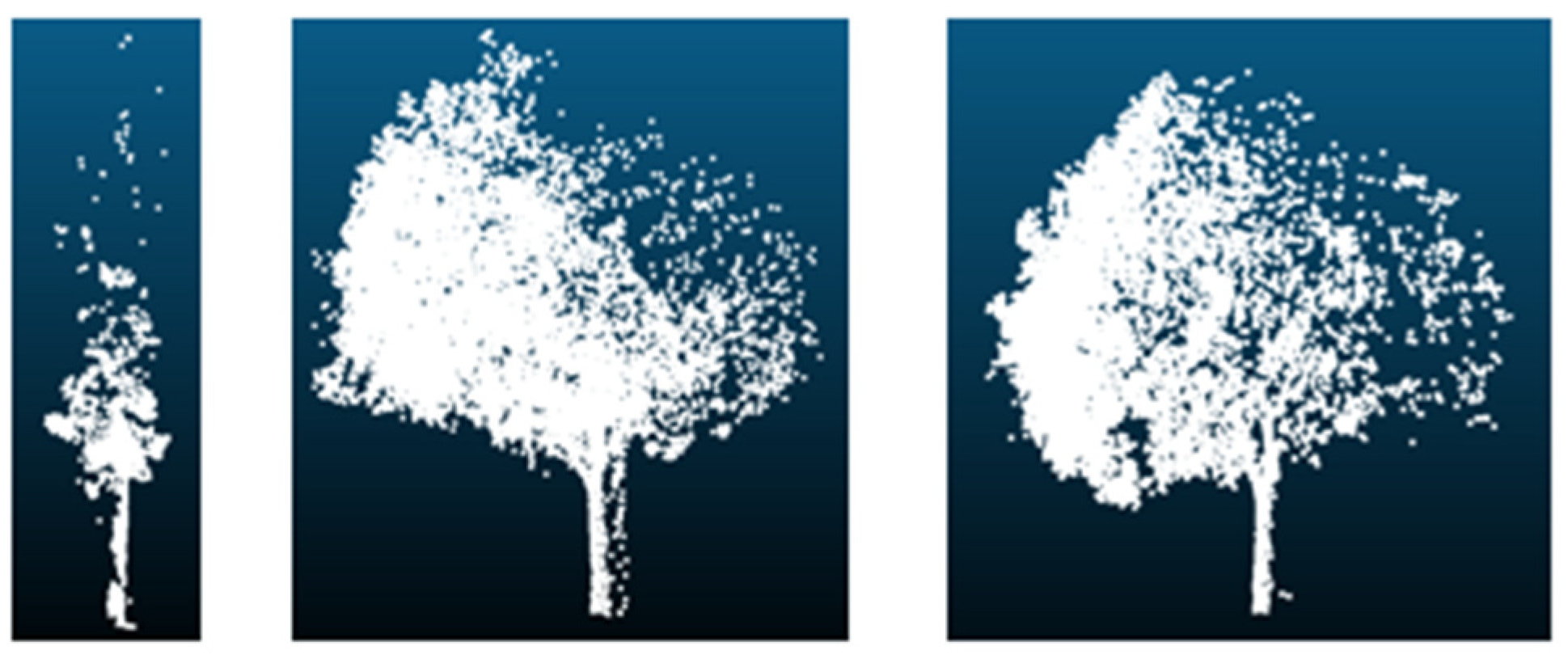
The quantitative bio-indicator calculation based on the single tree point clouds, for example, the biomass, tree height, and the crown diameter, depends on the integrity of their point clouds structure. However, the accuracy of these indicators may be affected by certain factors, such as the mutual occlusion of ground objects, insufficient penetration ability, and the accuracy of sensors. The sensor will be limited by the viewing angle of the collection equipment, for example, the vehicles can only drive along the road, resulting in the lack of complete viewing angle observation conditions for a considerable part of trees. Taking Figure 1 as an example, there is a missing canopy point clouds far from the direction of the mobile laser scanning (MLS) point clouds data. All these factors will directly lead to the loss of vegetation canopy point clouds, thereby indirectly affecting the accuracy of quantitative bio-indicator calculation. For instance, we need a complete single tree point clouds for accurate living vegetation volume (LVV) calculation [1] in this study of urban area LVV project.
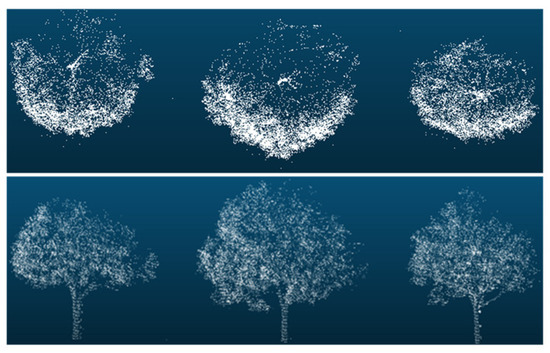
Figure 1.
Schematic diagram of the missing structure of a single tree point clouds obtained by MLS.
Point clouds structural completion has been intensively studied in the field of point clouds processing based on deep learning. For example, PF-Net [2] preserves the original point clouds and predicts the detailed geometric structure of the missing areas based on this. To ordinary point clouds objects, this type of method can effectively restore the detailed features of the missing point clouds. The primary topic of this study is to introduce the deep-learning-based point clouds structural completion into the field of forestry remote sensing, use the data-driven methods to complete the missing recovery of single tree point clouds, and validate it with the type of MLS point clouds. The reason for using MLS point clouds is that there are point clouds in this data source that have a relatively complete collection perspective and a basically complete point clouds structure, for example, the single trees located at road corners or parking lots, which can be used to construct complete (incomplete) tree pairs to train the structural completion models.
There are two difficulties in adopting the tree point clouds completion methods based on deep learning, as given in the following data. (1) The point clouds’ structure captured by MLS light detection and ranging (LiDAR) is characterized by the dense points near the sensor and the sparse points farther away. Therefore, the primary challenge is in designing a structural completion network that enables the model to learn and predict the missing structure of single tree point clouds. (2) The common point clouds completion is required to produce the pairs of missing point clouds and complete the point clouds for model training. For the convenience of writing, this process is briefly termed as constructing complete (incomplete) tree pairs. In the field of computer vision, the commonly used method for the point clouds completion has adopted the random spherical loss pattern. This method selects a sphere center in space and randomly eliminates the partial point clouds closest to the sphere center. However, the uneven density point clouds caused by the limited perspective, instead of spherical ones, forms the missing pattern of the real MLS point clouds data. As the distance from the vehicle’s track increases, the point clouds density will decrease owing to the obstruction of leaves or branches and the limited penetration of LiDAR.
To resolve the challenges posed by the current situation, our study undertakes the following works, namely, (1) by combining cutting-edge deep learning techniques like self-supervised and multiscale Encoder (Decoder), a TC-Net model suitable for the single tree structural completion has been proposed. In the model, the self-supervised module employs a data-driven approach to learn predicting the missing structure of a single tree point clouds, whereas the multiscale Encoder (Decoder) is employed to capture the semantic features of different spatial scales of a single tree point clouds and gradually predict the missing part of the point clouds. (2) Among the constructing processes of the single tree complete (incomplete) pairs to train the TC-Net model, the commonly used random spherical loss pattern in point clouds completion is not suitable for the single tree structure completion. Inspired by the penetration and attenuation of electromagnetic waves in a uniform medium, a data production method has been designed to simulate the missing of the real MLS point clouds, that is, an uneven density point clouds loss pattern has been proposed. Further, (3) we have extracted the structurally complete single tree point clouds from our self-collected MLS data, and a data set is constructed to train the TC-Net model with the uneven density point clouds loss pattern. We have realized the structural completion of single tree point clouds in real scenarios. Finally, we compare the structural completion results with the relatively complete point clouds reconstructed based on the airborne oblique photography images of the canopy to quantitatively demonstrate the completion effect.
The remainder of this paper is organized as follows. Section 2 gives a brief introduction to the related studies on the commonly used methods and deep-learning-based single tree structural completion in the field of forestry remote sensing. We detail our methodology in Section 3, including the implementation process of the proposed method, the network design of the TC-Net model, and the uneven density point clouds loss pattern for constructing the complete (incomplete) tree pairs. Section 4 details the experiments to test the accuracy of the single tree structural completion based on our approach, which accompany other supplementary performance comparison experiments, and discusses the results. Finally, the conclusions of this study and directions for future research in the field are provided in Section 5.
2. Related Studies
It is difficult to compensate the single tree completion owing to the factors, such as the spatial distribution of the urban features being complex, with a large amount of mutual obstruction, limited sensor accuracy, and penetration ability. Furthermore, the sensors may be limited by the observation angle of the collection device, resulting in the loss of tree point cloud structure. The methods of deep-learning-based completion and traditional single tree completion are intended for resolving this problem.
2.1. Traditional Single Tree Point Clouds Completion Method
Traditional point clouds completion methods can be divided into the geometry-based and model-oriented methods. The former requires the utilization of the geometric characteristics of objects, such as the continuity of the surface and the symmetry of the shape. Sarkar et al. have used the smooth interpolation methods to fill incomplete voids on the surface of point clouds [3]. Sung et al. have utilized the symmetry of the object to copy the unobstructed part of the point clouds to the missing part, thus completing the point clouds completion [4]. The geometry-based method requires that the missing part can be inferred from the unobstructed part. Hence, it is suitable for situations where the geometric shape is relatively regular and the data missing is not severe, besides the usage conditions being moderately adverse.
The model-oriented methods search for similar models by matching the incomplete object shapes with the models in large databases. Li et al. have employed the direct retrieval method to directly match the input with the model in the database for using it as the final completion result [5]. Martinovic et al. have employed the partial retrieval methods to divide the input into several parts, match the model in the database, and then combine the matching results to generate the final completed result [6]. To achieve better matching results, Rock et al. [7] have deformation-based methods to deform the retrieved shapes to obtain better matching of the input shapes. Furthermore, to reduce the algorithm’s dependence on the database, Mitra et al. [8] have employed the geometric primitive method to match with the input to complete the missing parts. Different geometric primitives have been utilized to represent and describe the shape features in point clouds, thus serving as the basic building blocks of point clouds structure, to better understand and represent the structure and shape features of point clouds.
Thus, the advantage of traditional methods is the ease of implementation using simple algorithms. The disadvantage is the inability to estimate the geometric shape of the missing area when the incomplete area of the input point clouds is larger.
The commonly used methods in the field of forestry remote sensing to resolve this problem can be broadly divided into three categories, namely, (1) multi-perspective/multi-sensor point clouds fusion method, (2) prior-based or modeling-based correction method, and (3) feature-based structural completion method based on the original single tree point clouds data.
In the first method given above, the point clouds fusion includes the multi-view fusion of ground-based LiDAR or backpack LiDAR and the weighted fusion of unmanned aerial vehicle (UAV) LiDAR and the backpack LiDAR [9]. The second traditional completion method, that is, the prior-based or modeling-based correction method, is primarily based on the prior or modeling of the tree skeleton. For example, Xu et al. [10] have first obtained the rough tree skeleton from the original missing point clouds, then the skeleton branches have been generated based on the canopy structure, and finally, the leaves are allocated to the corresponding positions of the skeleton to compensate for the modeling. Zhang et al. [11] have first obtained the visible skeletons from the original missing point clouds, and then the invisible skeletons based on hierarchical crown feature points are generated. Further, the two parts based on the particle flow method are finally combined to obtain the final tree model. In the third method, Mei et al. [12] and Cao et al. [13] first extract the key points from the missing point clouds based on the L1-Median algorithm, and then the point clouds completion is carried out based on the main direction of the extracted key points and the density distribution of the point clouds.
However, the point clouds fusion with the multi-perspective/multi-sensor point clouds fusion method, that is, the first method, relies on further data. These data are limited by the site and experimental conditions, and thus this factor can significantly increase the costs. The second and third methods cannot achieve an accurate completion, and there may be missing details in the completion part. Therefore, this study attempts to complete the single tree point clouds structural completion based on the emerging deep learning technologies.
2.2. Point Clouds Completion Based on Deep Learning
Point clouds structure completion is a key issue in the field of point clouds processing based on deep learning. For example, L-GAN [14] is carried out the point clouds completion based on the Auto-Encoder model and generative adversarial network. FoldingNet [15] has been designed as a foldable decoder to better restore the three-dimensional (3D) surface information of objects. PCN [16] combines the advantages of L-GAN and FoldingNet and incorporates post-processing operations that can make the results smoother, thus achieving better completion results. RL-GAN-Net [17] has combined reinforcement learning with a conditional generative adversarial network for steadily completing the large missing point clouds. PF-Net [2] has preserved the original point clouds and predicted the detailed geometric structure of the missing area based on this. Specifically, PF-Net has been designed as a multiscale pyramid-structured feature Encoder (Decoder) for the hierarchical estimation of the missing point clouds. The multiscale complement loss function has been designed to complete the back-propagation, and the corresponding discriminator and counter-loss function was designed to achieve a better training process. TopNet [18] has been designed as a hierarchical tree structure Encoder to achieve the completion. DPGG-Net [19] has been designed as two modules based on the generative adversarial network. Further, the point clouds completion task has been transformed into the point clouds global feature generated from the missing point clouds by Decoder, with the countermeasure training task of global feature in the point clouds completion. Furthermore, PMP-Net++ [20] has considered the point clouds completion task as a deformation one, thus predicting the complete point clouds by moving the missing point clouds three times. During the movement process, the total movement distance will be minimized, and the result of each movement will be employed as the output of the next movement. Especially in recent years, the point-based, convolution-based, folding-based, graph-based, generative-model-based, and transformer-based methodologies have also been developed [21]. These approaches are increasingly being applied to complete and reconstruct point clouds of various objects across a wide range of fields. For example, Ibrahim et al. [22] applied point clouds completion in the context of vehicles, Toscano et al. [23] used in dentistry, and Sipiran et al. [24] used in the cultural heritage. However, most of the initial models are trained using point clouds of artificial objects that have clear continuity and symmetry characteristics [25].
In the field of forestry remote sensing, Li et al. [26] have proposed a completion network framework by employing an Encoder (Decoder) for the problem of plant leaf completion. Xiao et al. [27] have proposed a completion network based on multiscale feature extraction, which inputs the extracted global features into a Decoder combined with a point clouds pyramid to generate a single leaf point clouds in multiple stages. Jiang et al. [28] have proposed a method for supplementing plant skeletons, which first employs a local iteration method based on L1 median to extract the skeleton and uses a Bezier curve to fit the missing parts of the stem. Cai et al. [29] proposed an effective algorithm that extracts branches through the region growth, eliminates incorrect branches based on specific features, and reconstructs them using the polynomial fitting. Pan et al. [30] have employed a simple Encoder (Decoder) to supplement multiple plants in the farmland to calculate the total biomass of the farmland. Finally, it was utilized to calculate the total biomass. Xu et al. [31] have developed a model based on PointNet and EdgeConv, for orchard trees using data collected from agricultural robots. However, the potential of deep learning for completing morphologically complex natural objects, such as trees, remains uncertain.
Although the abovementioned models can effectively complete the missing point clouds to a certain extent, there is still incomplete feature extraction of point clouds structures and missing details of the completed point clouds, besides a lack of effective expression of local feature information on the object surface. Concomitantly, under the conditions of sensor noise, sparse point clouds, and ground occlusion, the structure of these models is sophisticated, which results in problems such as the lack of robustness of the models. These models primarily focus on the point clouds completion of ordinary objects, thus making it difficult to directly apply them for the vegetation point clouds processing. Therefore, the introduction of point clouds structure completion based on deep learning into the field of forestry remote sensing is the focus of this study. To carry out the structure completion of single tree point clouds, we employ a novel data-driven method, that is, constructing a deep learning network model.
3. Methodology
This section focuses on our overall research approach, the construction of the TC-Net network, and the proposal of a new missing method and a local similarity visualization method for the vegetation point clouds.
3.1. Research Approach
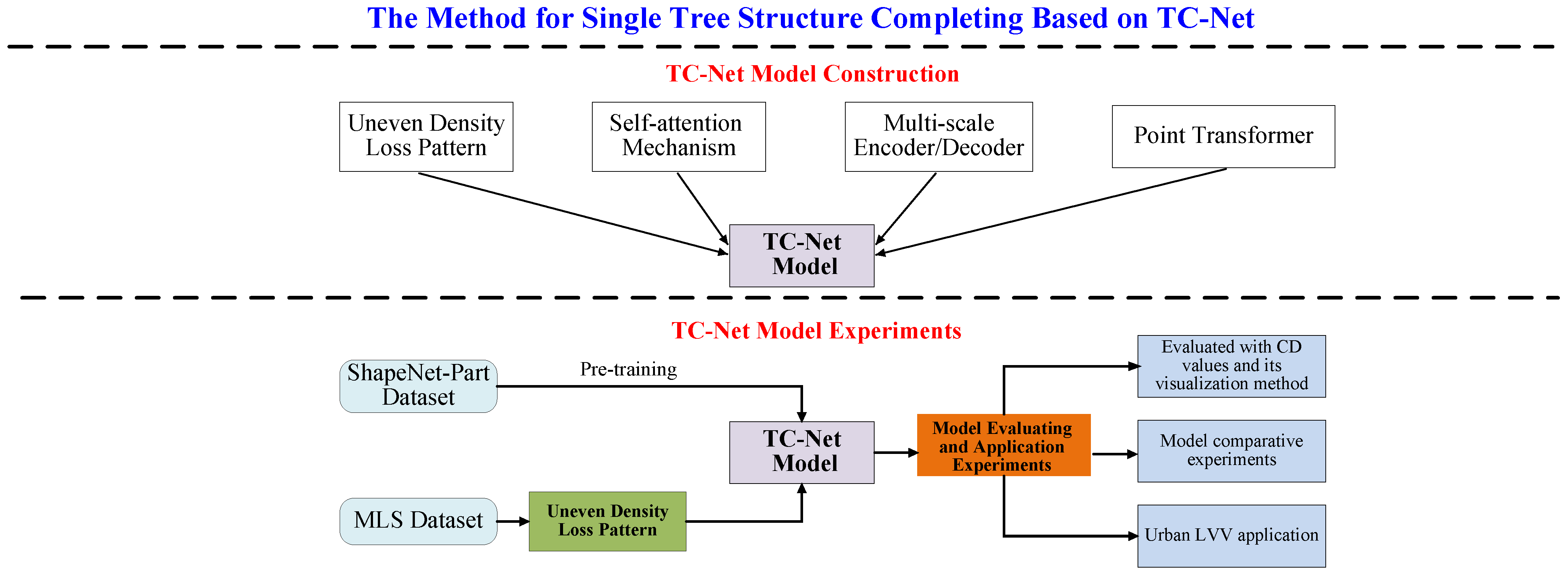
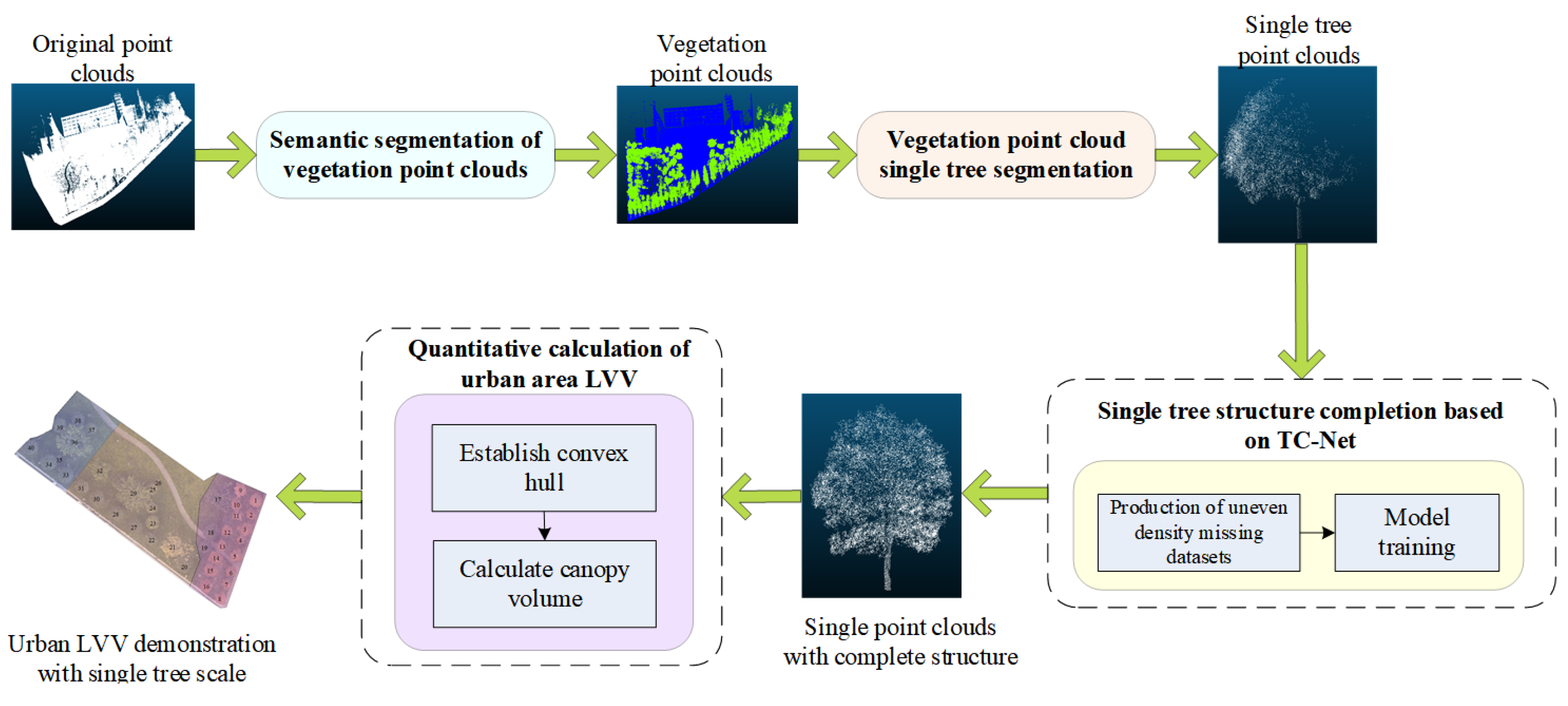
In response to the above issues, our approach proposed in this study is depicted in Figure 2. The entire approach is divided into two parts to answer the following questions regarding (1) the design and construction of a TC-Net model and (2) the method for efficient completion of the training of the model, besides the relevant design experiments that effectively validate the TC-Net model.

Figure 2.
Overall research approach.
According to Figure 2, for the construction of the TC-Net model (see the upper part of Figure 2), this study combines Self-Supervised and MultiScale Encoder (Decoder) deep learning techniques to fill the gap in deep-learning-based single tree completion research. Further, it employs Transformer to extract weighted features and designs a multiscale encoding and decoding TC-Net model suitable for the single tree structure completion. Concomitantly, this study proposes a dataset production method suitable for MLS data sources, termed the uneven density point clouds loss pattern, to ensure the alignment of the trained model with the real-world application scenario.
In terms of the experimental design for TC-Net model validation (see the lower part of Figure 2), first, the pre-training techniques have been employed to train the TC-Net model based on the ShapeNet-Part dataset. The trained TC-Net model has been obtained based on the construction of dataset training by employing the method of uneven density point clouds loss. Thereafter, the experiments of the missing single point clouds data from the test set and actual scenarios have been carried out, and the completion accuracy of the model using Chamfer distance (CD) values is evaluated. Concurrently, the model is applied in practice, thereby verifying its effectiveness and practicality when combined with the specific urban area LVV project.
3.2. Construction of TC-Net Model
This section will combine the cutting-edge deep learning techniques, such as self-supervised mechanisms and multiscale Encoder (Decoder) structure. We adopt a network framework similar to PF-Net to propose a novel Tree Completion Net (TC-Net), which is suitable for single tree structure completion in forest remote sensing. According to Figure 3, the self-supervised module refers to the manual construction of the complete (incomplete) tree point clouds pairs. This is to enable the model to learn how to generate the corresponding complete point clouds based on the incomplete point clouds for a single tree. Henceforth, it learns to predict the missing structure of the single tree point clouds based on data-driven methods. The multiscale Encoder (Decoder) module is employed to capture the semantic features of a single point clouds at different spatial scales and gradually predict the missing parts of point clouds.

Figure 3.
Specific structure of TC-Net.
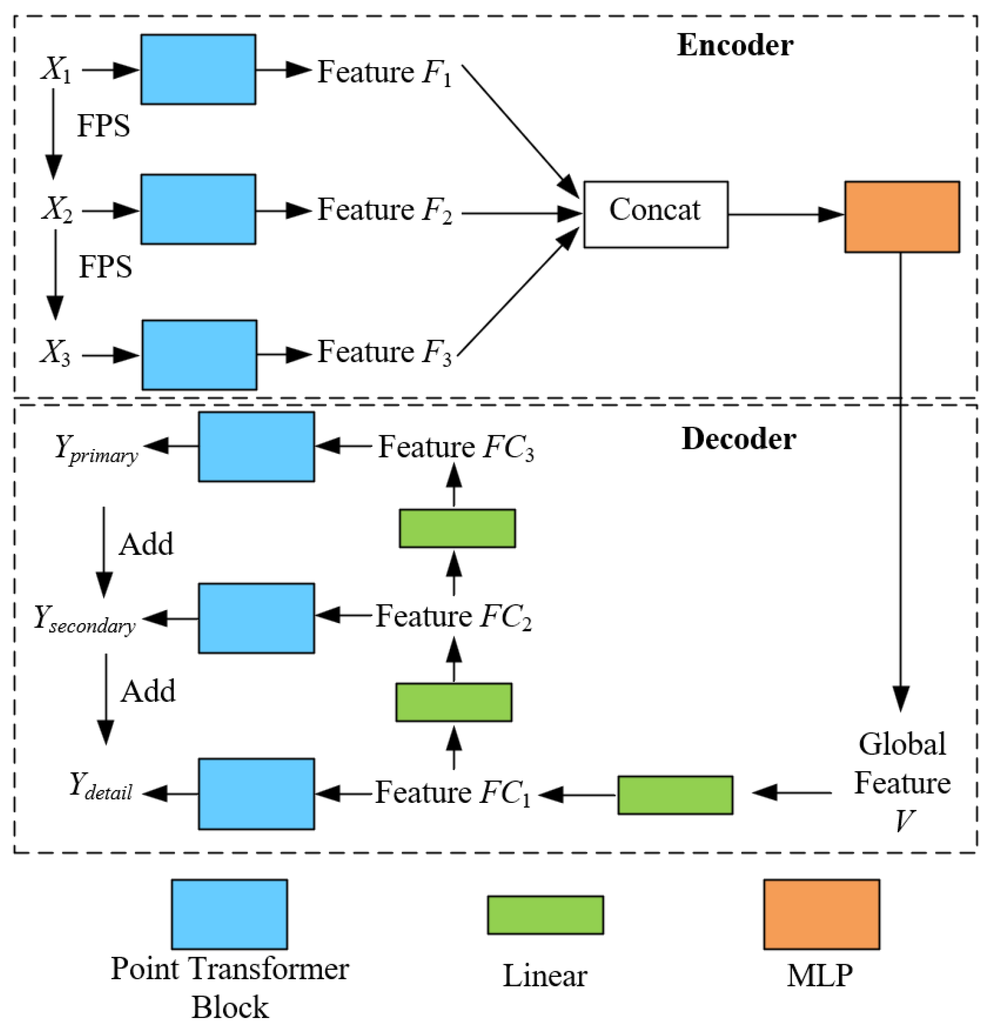
According to Figure 3, the entire network structure of TC-Net is composed of two parts, namely, Encoder and Decoder. To the Encoder part, its specific principle is given as follows. (1) First, by using fastest point sampling (FPS) [32], we can obtain the three resolution down-sampled incomplete point clouds Xi (i = 1, 2, 3, with N, N/k, and N/k2 points, respectively), and the corresponding missing completion point clouds Yi (i = 1, 2, 3, with M, M/k, and M/k2 points, respectively). Compared to the random sampling, the point clouds obtained by FPS can better represent the overall distribution of the missing point clouds. In this context, assuming the input point cloud is , each point possesses features in , implying that each point has c-dimensional features. The FPS method selects a subset from these points, denoted as , where this subset contains the m points that are the farthest apart in linear space. By selecting these farthest points, the overall geometric distribution of the point cloud is better preserved, thus ensuring that the down-sampled point clouds retains stronger representativeness.
Thereafter, the hierarchical semantic features are extracted using a multi-resolution Encoder with three different sampling rates point clouds. The multi-resolution point clouds first pass through the point Transformer layer to obtain the feature Fi (i = 1, 2, 3) and then employs multilayer perceptron (MLP) to fuse the features to obtain the vector V of the global spatial semantic features. The point Transformer layer uses offset-attention [33] mechanism to calculate the semantic similarity between different point clouds features for the semantic modeling. Thus, predicting the residual blocks instead of the features themselves can achieve better training results by assuming that Query, Key, and Value are set to Q, K, and V, respectively. The principle of offset-attention is given as follows:
where and . and are a learnable linear transformation shared by this layer. Among them, , , and R is an adjustable hyperparameter. Further, and represents the number of feature points and dimensions for each spatial-scale layer, respectively. The output calculation of the attention layer, that is, , is given as follows:
where A represents the attention score, whereas LBR indicates that the feature first passes through the linear layer, then through the BatchNorm layer, and finally output by the ReLU layer.
To the Decoder part, inspired by PF-Net [2], we employ the multiscale generative networks to gradually predict the missing point clouds. Starting from V, three feature layers FCi (i = 1, 2, 3) have been obtained through a linear layer. The deepest FC1 will be converted to the first predicted point clouds Yprimary through the point Transformer layer. FC2 is employed to predict the relative coordinates of the second layer of point clouds Ysecondary, that is, with each point in Yprimary as the center, the relative coordinates of the corresponding point are in Ysecondary. FC3 is used the same as FC2 to predict the relative coordinates of Ydetail with respect to Ysecondary. Further, Ydetail will serve as the final output to predict the missing point clouds structure. The number of points for Yprimary, Ysecondary, and Ydetail is M, M/k, and M/k2, and corresponds to Y1, Y2, and Y3, respectively.
In the TC-Net model, the loss function is a multiscale compensation loss, which is composed of the weighted CD of predicted point clouds, namely, Ydetail, Ysecondary, and Yprimary and (Y1, Y2, Y3). Chamfer distance is a distance measurement method between the point clouds that can be employed to evaluate the similarity between two different point clouds data sets. Its basic idea is to calculate the minimum distance, point by point, from one point set to another point set, and then obtain the average minimum distance. The formula for this process is given as follows:
Here, represents the adjustable hyperparameters. Thus, the specific calculation of the CD value, that is, , is given as follows:
where and represent two-point clouds and represents the Euclidean distance.
Accordingly, the TC-Net model first obtains different spatial-scale features of the incomplete point clouds based on the multiscale Encoder and fuses them to obtain the global features. Then, the model learns to generate corresponding complete single tree point clouds based on the incomplete single tree point clouds by using the multiscale Decoder to transform the global features into the missing point clouds, that is, realizing the study of a single tree structure completion.
3.3. Pattern for Simulating Uneven Density Loss of Real MLS Point Clouds
One import step, that is, manually constructing a complete (incomplete) single tree point clouds pair, is required to complete the entire data-driven single tree structure completion. Furthermore, the constructed missing effect should be identical to the missing single tree structure in the real MLS point clouds. Accordingly, the model can learn to identify and compensate for the missing structure in the real scene, that is, fulfill the single tree structure completion task with a self-supervised method.
In the field of computer vision, adopting the random spherical missing pattern is the commonly employed method for creating the missing point clouds. In this missing pattern, it randomly selects a spherical missing point clouds in space and randomly eliminates the part of the point clouds closest to the spherical center. Thus, it eliminates the overall 25% points. The visualization effect is depicted in Figure 4 [34].
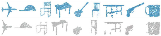
Figure 4.
Schematic diagram of the random spherical missing point clouds pattern. The blue point clouds above represent the complete point clouds, and the gray point clouds below represents the missing point clouds.
During the process of collecting point clouds data with the MLS system, the missing mode of the real vehicle point clouds data is not the spherical missing; instead, it is the way of uneven density point clouds missing caused by the limited viewing angles and gradually decaying penetration of LiDAR. As the distance from the vehicle’s trajectory increases, the point clouds density will decrease owing to the obstruction of leaves or branches, combined with the limited laser radar penetration, according to Figure 5. The missing patterns that do not match will prevent the deep-learning-based point clouds completion model from completing smoothly.

Figure 5.
Schematic diagram of the missing mode of real MLS point clouds data.
We propose a new missing method, that is, the uneven point clouds density loss pattern, to construct a similar missing effect with Figure 5, being inspired by the attenuation of electromagnetic waves through a uniform medium [35]. First, we take the formula for the attenuation of electromagnetic waves through a uniform medium, as given below:
where I is the current electric field intensity (in V/m), I0 is the original electric field intensity (in V/m), μ is the propagation attenuation coefficient of the homogeneous medium (related to the physical properties of the homogeneous medium and the electromagnetic wave frequency and wave speed, unit is m−1), and d is the propagation distance of the electromagnetic wave relative to the original position (unit: m). The electric field strength of the electromagnetic wave in the homogeneous medium suffers an exponential decay. Correspondingly, when migrating this attenuation scene to that of MLS data collection, that is, a vehicle-mounted LiDAR device, the primary attenuation is considered the attenuation of electromagnetic waves emitted from the LiDAR in the tree canopy. The uneven density point clouds loss pattern has been proposed according to the attenuation associated with the probability of point clouds missing, as given below:
where p represents the probability of the target point clouds appearing in the missing dataset, is 1, is the given attenuation parameter, and d is the distance between the line of the vehicle-mounted LiDAR and the target point clouds passing through the tree canopy. Thus, it represents the maximum probability when there is no canopy barrier between the point clouds and the vehicle-mounted LiDAR device. Further, it becomes an exponential decay attenuation with the distance through the canopy.
This study sets d as the distance between the target point clouds and the vertical line representing the vehicle’s travel line passing through the tree canopy, after considering that the onboard LiDAR will travel along the road during the data acquisition. According to Figure 6, the blue point clouds represent the collection vehicle, and the corresponding red line represents the vehicle’s travel line, whereas the green point clouds represent the tree point clouds. Among them, P is the target point clouds, the white solid line represents the vertical line between the target point clouds and the vehicle’s travel line, whereas d is the distance that the vertical line passes through the tree canopy, and M is the edge of the tree canopy.
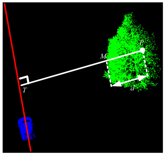
Figure 6.
Schematic diagram of uneven density loss mode.
The specific calculation of this loss pattern is given as follows. (1) We assume that the input complete point clouds quantity is 2048 points and the missing point clouds quantity is 512 points. (2) We find the vertical point T of P corresponding to the driving line and then find the length d of the vertical line segment . Accordingly, we calculate in sequence and get for all 2048 points, as given below:
(3) Further, we employ linear normalization (values taken as [0~1]) for all to obtain the approximate distance through the canopy, that is, d. A segmented probability approach has been adopted to maximally fit the real situation and accelerate the computational efficiency. First, we calculate the d of all points and sort them. The previous point clouds will be directly retained as , which meets the conditions ( [0, 1536)). The final point clouds are directly added to the missing part as , and these point clouds meet the condition of [0, 1536). And , meets the conditions: . The formula is given below:
The middle point clouds ( 2048) will be normalized by the distance d and converted into probability p according to Equation (6). Utilizing the PyTorch (version: 1.9)’s vector conversion function, we subtract the vector T with the length distributed in [0, 1] to obtain a new probability , as given below:
Further, the 512 lowest medium probability, among the new , will be added to the missing parts, as given below:
Finally, the missing point clouds is given as follows:
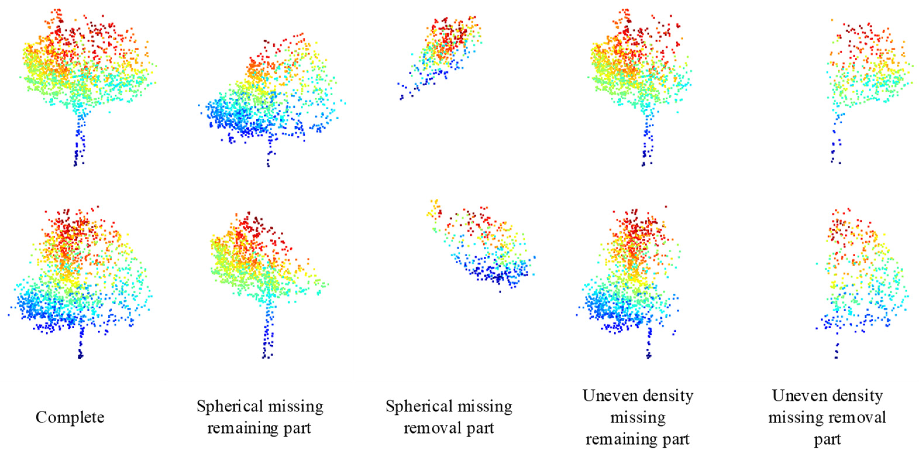
The missing situation closer to the real ones indicates a better model that can learn to predict the missing point clouds. According to Figure 7, it is a comparison between the random spherical missing pattern and the uneven density point clouds loss pattern achieved in this study. Here, the uneven density parameters are, namely, = 1024, = 256, and the attenuation parameter = 2. Comparing the 3rd column with the 5th column in Figure 7, the new loss pattern is closer to the real-world data.
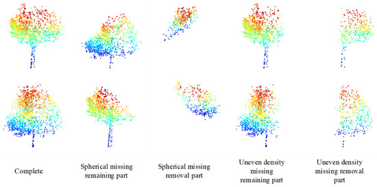
Figure 7.
Schematic diagram of the uneven density loss mode.
3.4. Local Similarity Visualization Method of Point Cloud
Chamfer distance (CD) is an index to evaluate the completion effect of point clouds as a whole, which quantitatively indicates the geometric difference between the predicted point clouds and the reference point clouds. However, this holistic assessment may not reflect the importance of local features and their distribution in practical applications. Therefore, this study proposes a local similarity visualization method of point clouds, which aims to visualize the chamfer distance and introduce visual auxiliary judgment to show the effect of tree completion from the local part under the premise of ensuring the objectivity of CD value. Next, the physical meaning of CD value in point clouds analysis will be discussed, and then the specific method for visualizing the CD value will be described in detail.
The calculation formula for the CD value is given as follows:
where and are the two-point clouds, represents the number of points of in the point cloud, and represents the Euclidean distance.
Equation (12) includes two parts, where one part is shown in Equation (13). It starts from the source point cloud , performs distance calculation on each point in and each point in the target point cloud , and selects the distance value of the point with the smallest distance, that is, , as the attribute value of the corresponding point in . The other part, as shown in Equation (14), starts from the target point cloud , computes the average distance , and follows the same steps performed as in the first part.
Being motivated by the physical meaning of CD values mentioned above, this study proposes a local similarity visualization method for point clouds as follows. Based on the complete point clouds P (true value), for each point in P, we find the distance of the point closest to in the completion point clouds Q, and the expression is shown in Equation (15).
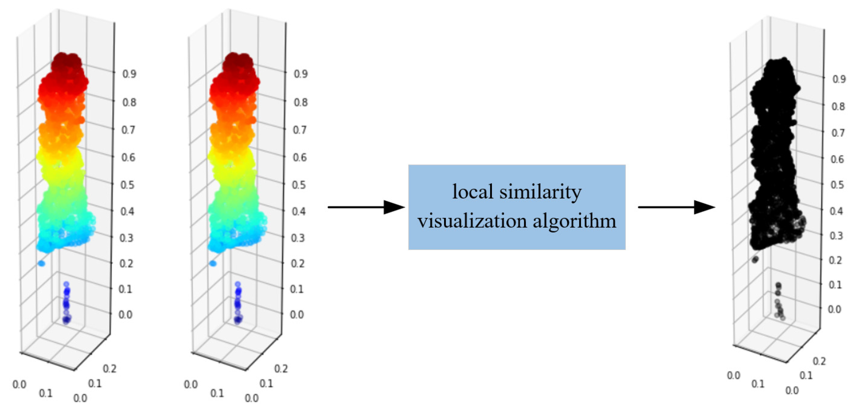
The visualization principle of Equation (15) is as follows. It starts from a specific point and describes the local similarity between point clouds. If , it indicates that one of the points in point clouds P has a completely corresponding point in point cloud Q. Then, is used as the attribute value of the point clouds and attached into the truth point clouds P, where its attributes are , where is the coordinate information of the point clouds P. Finally, the true value point clouds P is visualized, rendered with the fourth dimension, that is, the value of . The point in the true value point clouds P that is close to black indicates that there is a corresponding point in the predicted point clouds Q that is proximate to that point. The clustered points in point clouds Q cannot be found, when the point is proximate to the bright color.
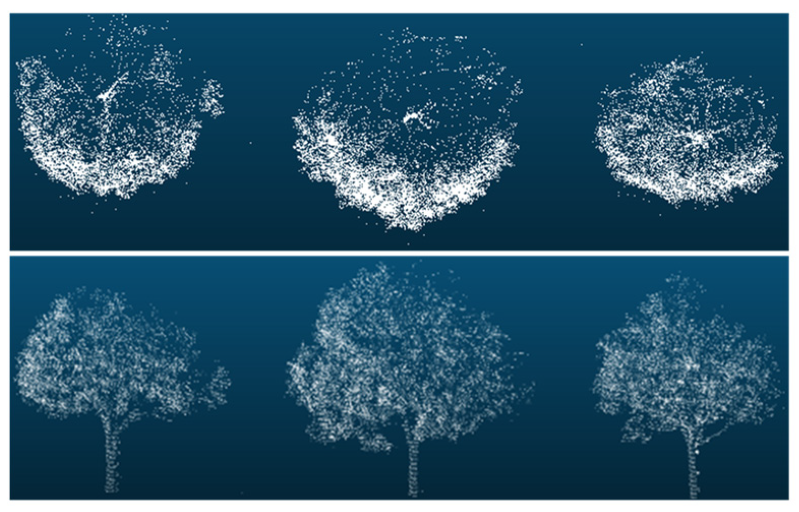
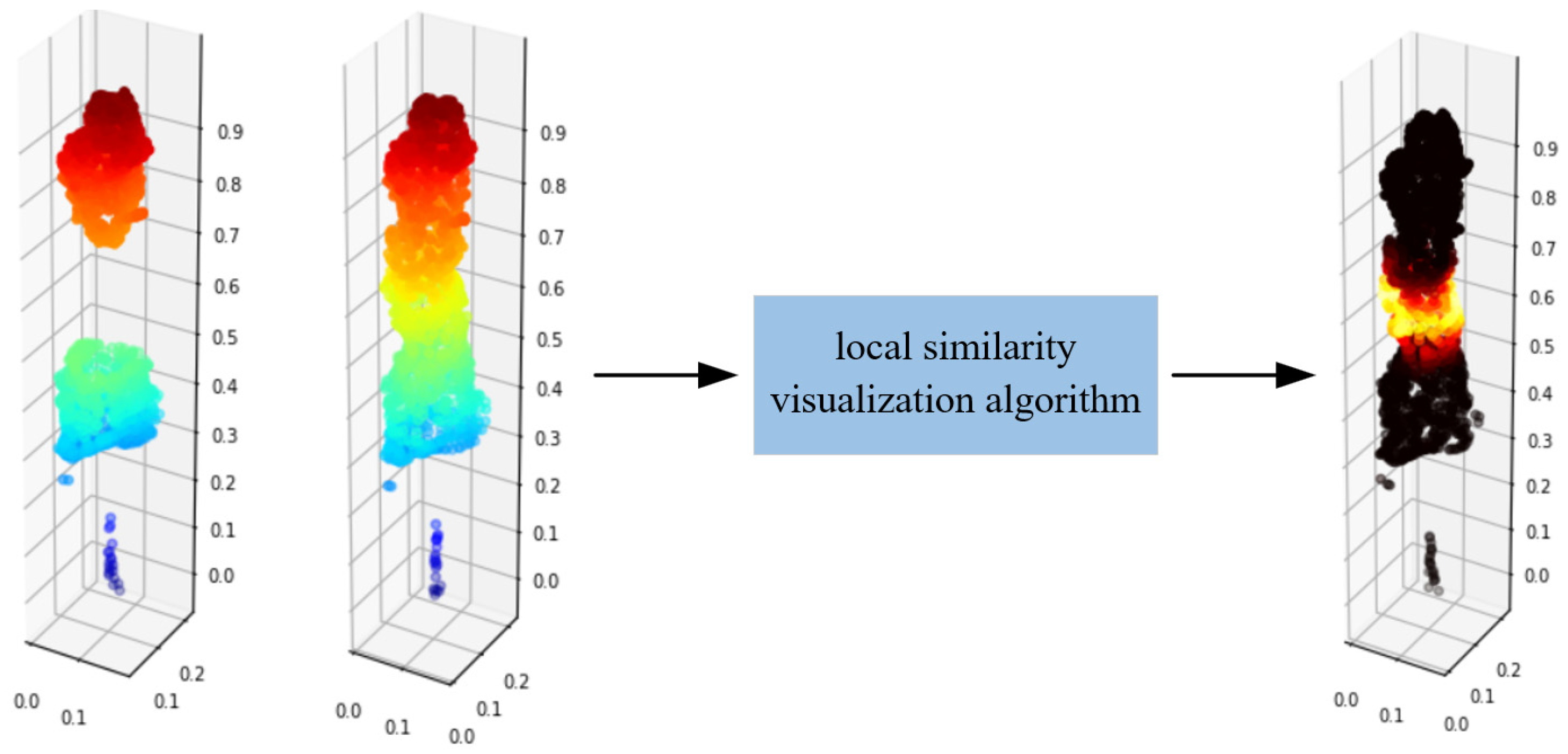
Based on this, the completion effect of point clouds can be visualized. According to Figure 8, the same point clouds P is input into local similarity visualization algorithm, and the output point clouds are all black, thus indicating a very high similarity of the two inputting point clouds. When the incomplete point clouds P and the complete point clouds P are input into the algorithm, as shown in Figure 9, the missing parts are bright, thus indicating that this part has a low local similarity.

Figure 8.
Local similarity visualization of complete point clouds.

Figure 9.
Local similarity visualization of incomplete point clouds.
4. Result
This section focuses on parameter setting, dataset production, and validation experiments of our proposed TC-Net method. Furthermore, the supplementary comparison experiments and the TC-Net’s practical application verification experiment are also presented.
4.1. Experimental Parameter Settings
The training of TC-Net is based on the pre-training of PF-Net. Based on comparative experiments or empirical values, in the experiment, the number of incomplete area points N of PF-Net is set to 1536, and the number of missing area points M is set to 512. Further, the down-sampling rate k is set to 2, and the multiscale complement loss function super parameter is set to 0.1. We use Batch Normalization and the RELU activation function. Furthermore, the optimizer uses Adam, with an initial learning rate lr = 0.001, a weight decay rate of 10−4, and a batch size of 32. Each training runs 200 epochs, and the model from the last epoch is taken as the final weight. We have built the entire code engineering based on PyTorch [36] and completed the entire training and testing by employing a 40 GB NVIDIA A100 graphics card.
There are two main sets of hyperparameters with the uneven density loss pattern. One is the lane line selection, and the other is the selection of the missing parameters, that is, , , and . The lane line scheme set in this study is given in the following data. While we input the point clouds data, normalization is first performed, and the xyz coordinates fall in the range of 0 to 1, occupying a cubic space with all sides 1. The lane line is randomly one of the four bottom edges of the cube. According to the parameter comparison experiment that we have conducted, the missing parameter scheme is given as follows: taking random integers ranging from 768 to 1280, taking random integers ranging from 128 to 384, and taking a random integer ranging from 1 to 4. Unless otherwise specified, these parameters will be used in all subsequent experiments.
4.2. Production of Self-Collected Single Tree Point Clouds Dataset of MLS
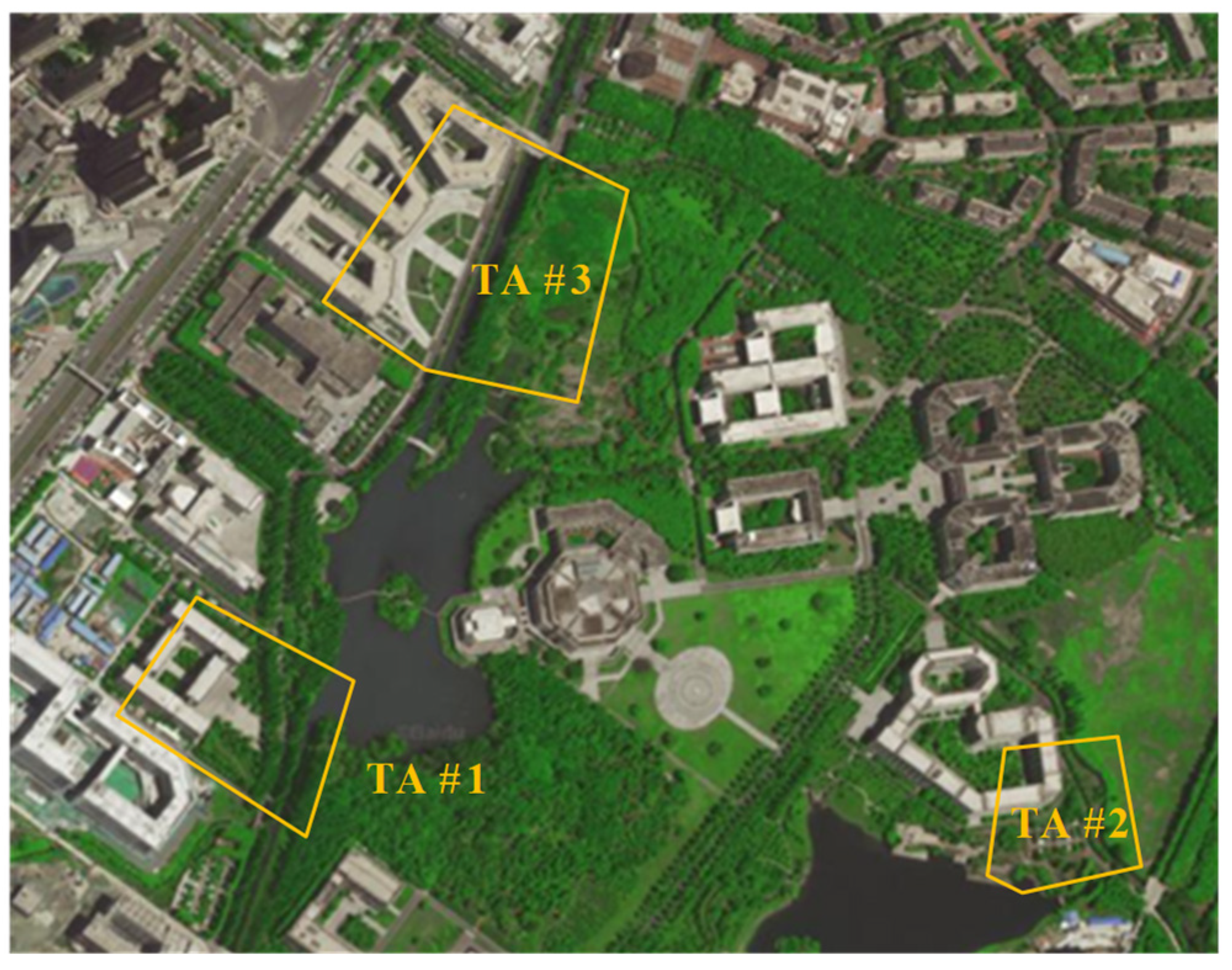
After a comprehensive consideration, the experimental area is selected at the Qingshuihe Campus of the University of Electronic Science and Technology (UESTC), which is divided into three measurement areas, namely, testing area #1 (TA #1), testing area #2 (TA #2), and testing area #3 (TA #3), as shown in Figure 10.

Figure 10.
Distribution of the three test areas in the experiments.
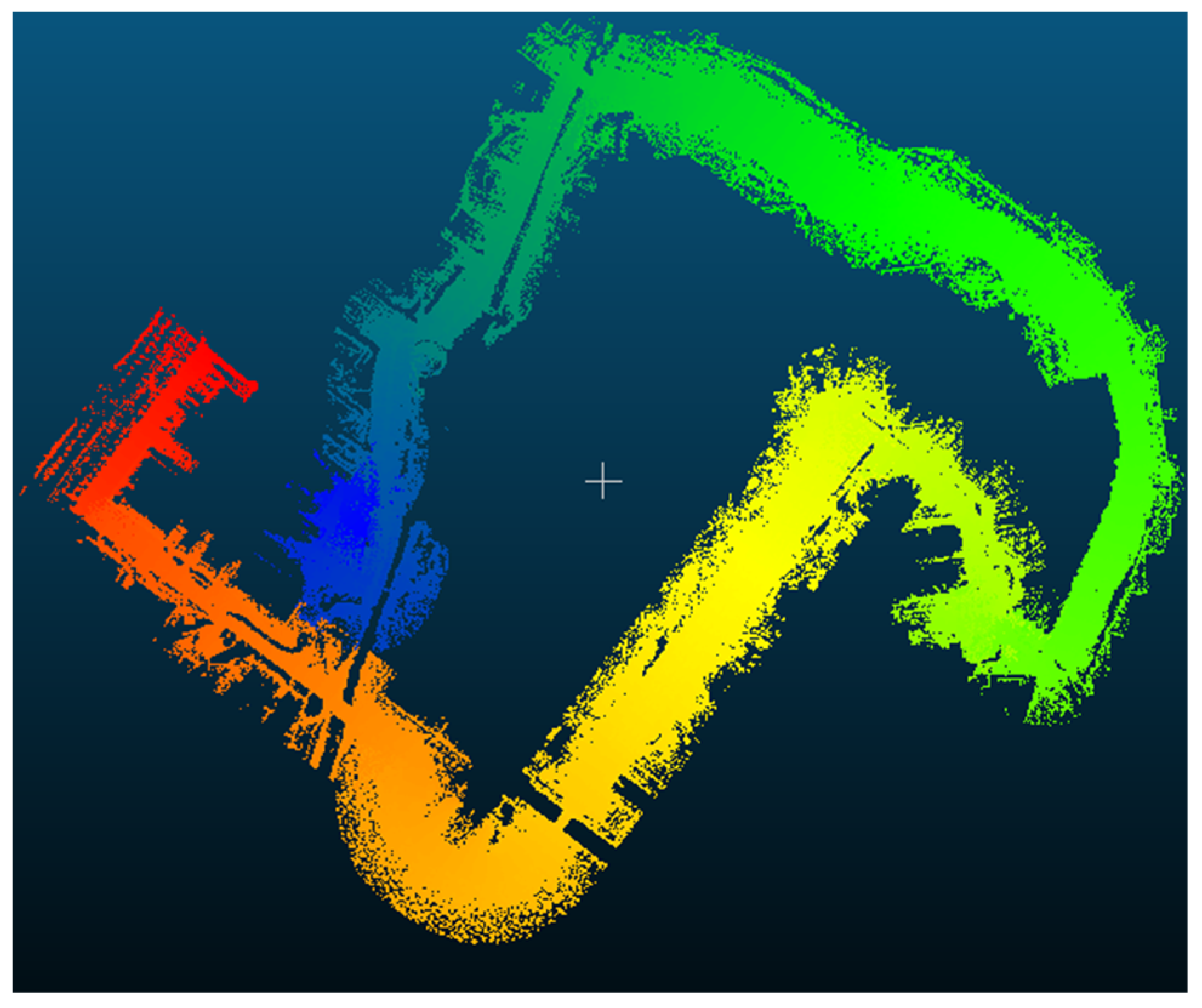
In the procedure of MLS data collection, a 128-line LiDAR device has been employed, and the LiDAR is fixed on the roof of the acquisition vehicle. The acquisition vehicle drives along the road in the experimental area to collect the original point clouds data. Following the processing, the static point clouds is obtained, with a spatial resolution of 5 cm and no color information, as shown in Figure 11.

Figure 11.
Self-collected MLS point cloud data set.
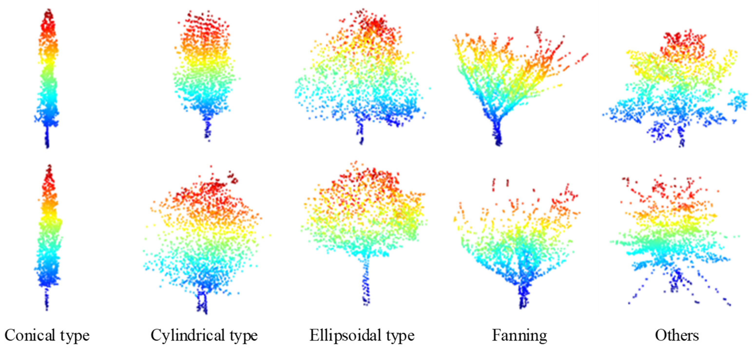
In the self-collected MLS point clouds data, after processed with a specially designed vegetation semantic segmentation model [37], the tree point clouds is separated from the original vegetation point clouds. Therefore, there are a few tree point clouds (such as single tree located at road corners or in parking lots) with a relatively complete collection perspective and a basically complete point clouds structure, which can be used as the initial complete input for TC-Net training. We manually filter the self-collected MLS point clouds of the entire test area and obtain a complete single tree point clouds, as shown in Figure 12, which only accounts for a small part of the entire data and is divided into cone type, cylindrical type, ellipsoid type, fan type, and others. Moreover, 139 of them are designated as the training samples and 33 as the test samples. The detailed information is shown in Table 1.
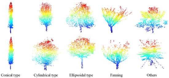
Figure 12.
Display of the complete tree point clouds data, which are collected by our MLS equipment and are all down-sampled to 2048 points using the FPS algorithm.

Table 1.
Detailed information of the training and test single tree point clouds sets with different types.
4.3. Single Tree Structure Completion Experiment Based on TC-Net and Uneven Density Point Clouds Loss Pattern
In the training procedure, this study employs our proposed uneven density missing pattern to train the model to solve the problem of missing patterns that do not match in real scenarios and prevent the model from completing smoothly. Further, a pre-training method is adopted, which employs the training parameters obtained from the ShapeNet-Part in the previous section as the initial parameters to compensate for the problem of insufficient data for single tree completion.
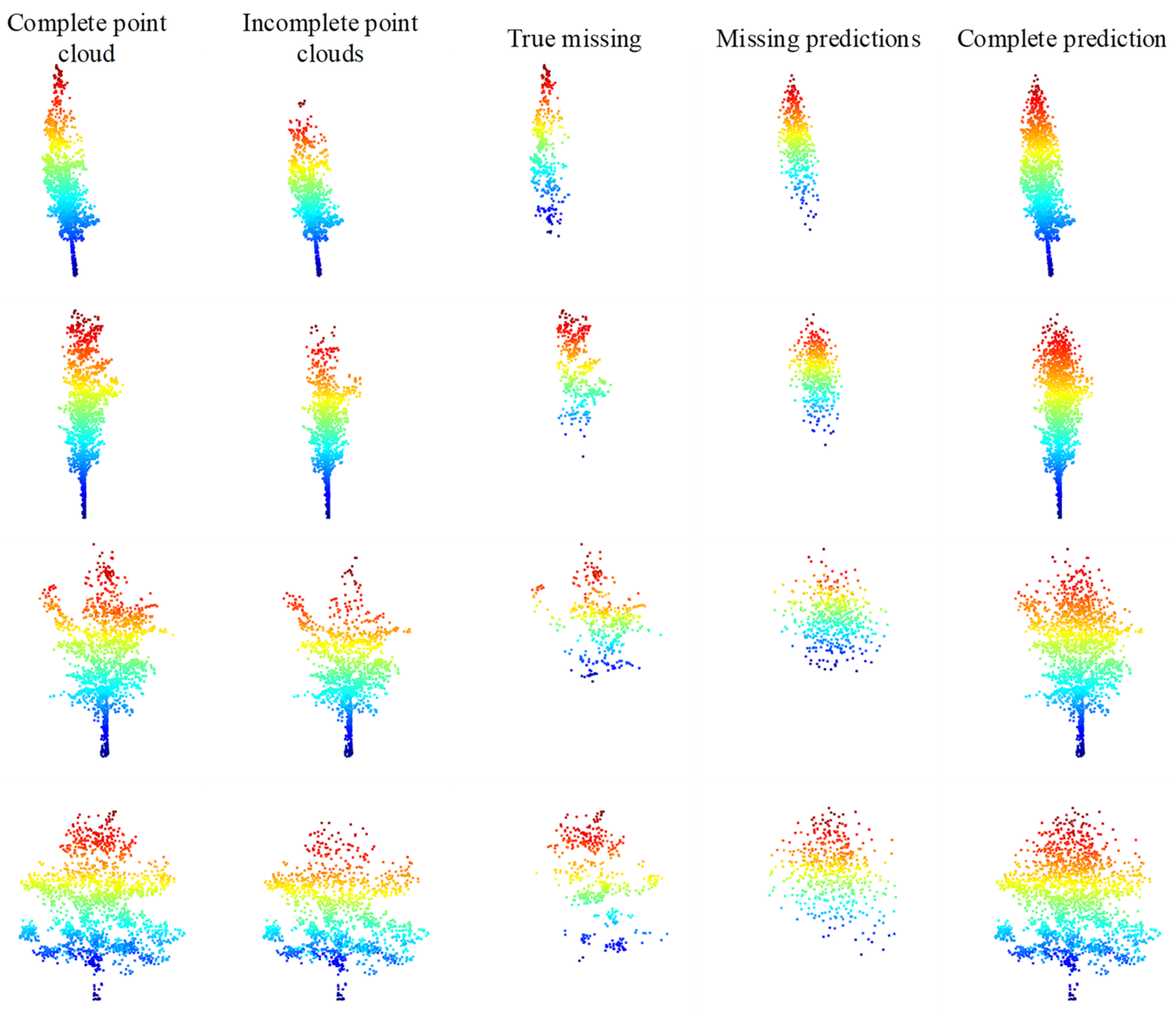
We have adopted the initial weights obtained from the training on ShapeNet-Part [38] to train the TC-Net model based on the uneven density point clouds loss pattern. The training data employs the collected data with a complete single tree point clouds in Section 4.2, that is, the involved point clouds, including a total of 139 complete single trees. First, we employ the trained TC-Net model to test on the testing data set provided in Section 4.2. We employ the uneven density missing pattern to create incomplete point clouds, and then employ the trained model for prediction based on the complete point clouds of the testing set. Taking four of them, the visualization effect is depicted in Figure 13. Accordingly, it indicates that the TC-Net model can effectively fulfill the completion task on the testing set.

Figure 13.
Test results of training TC-Net based on density loss pattern.
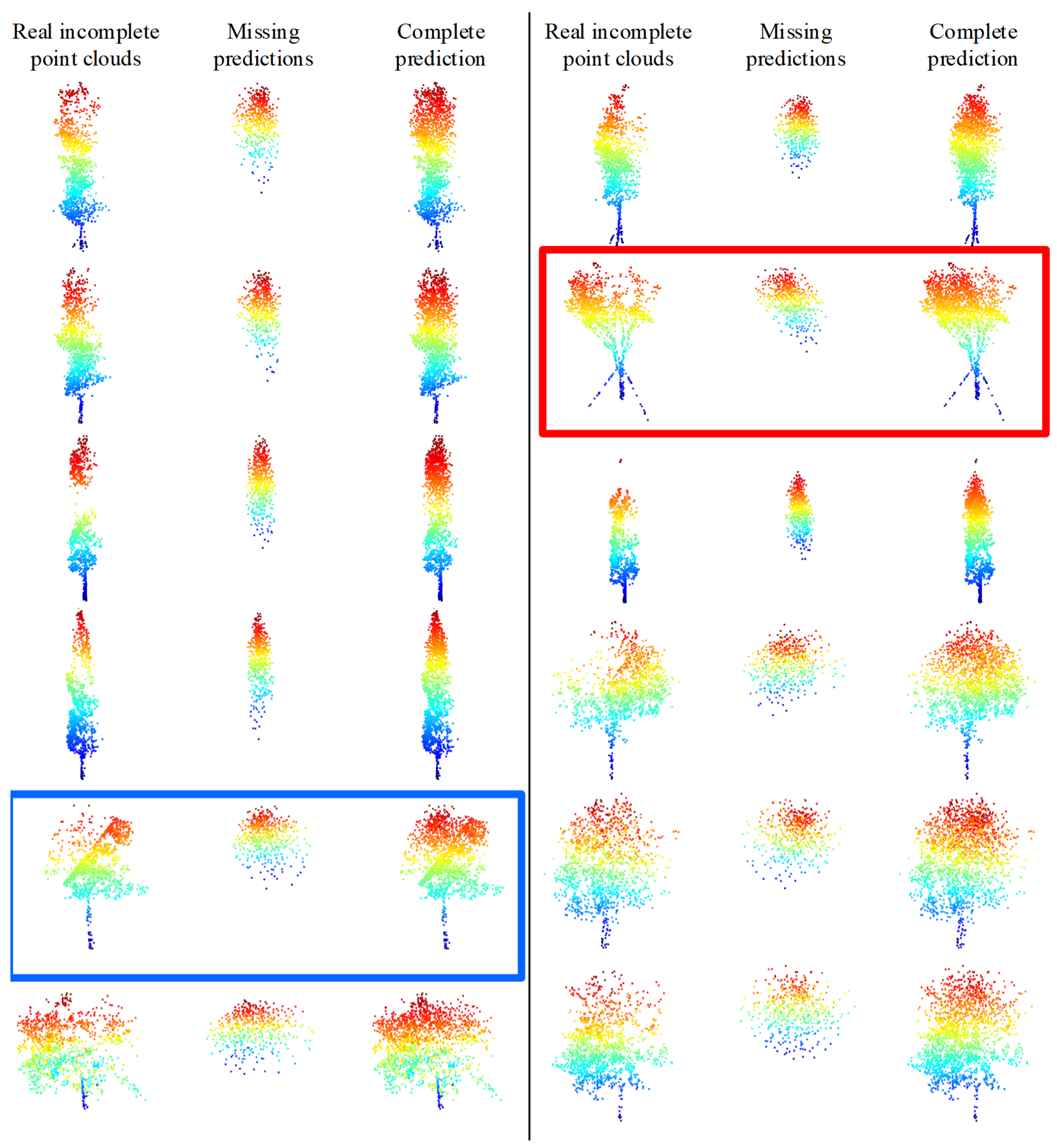
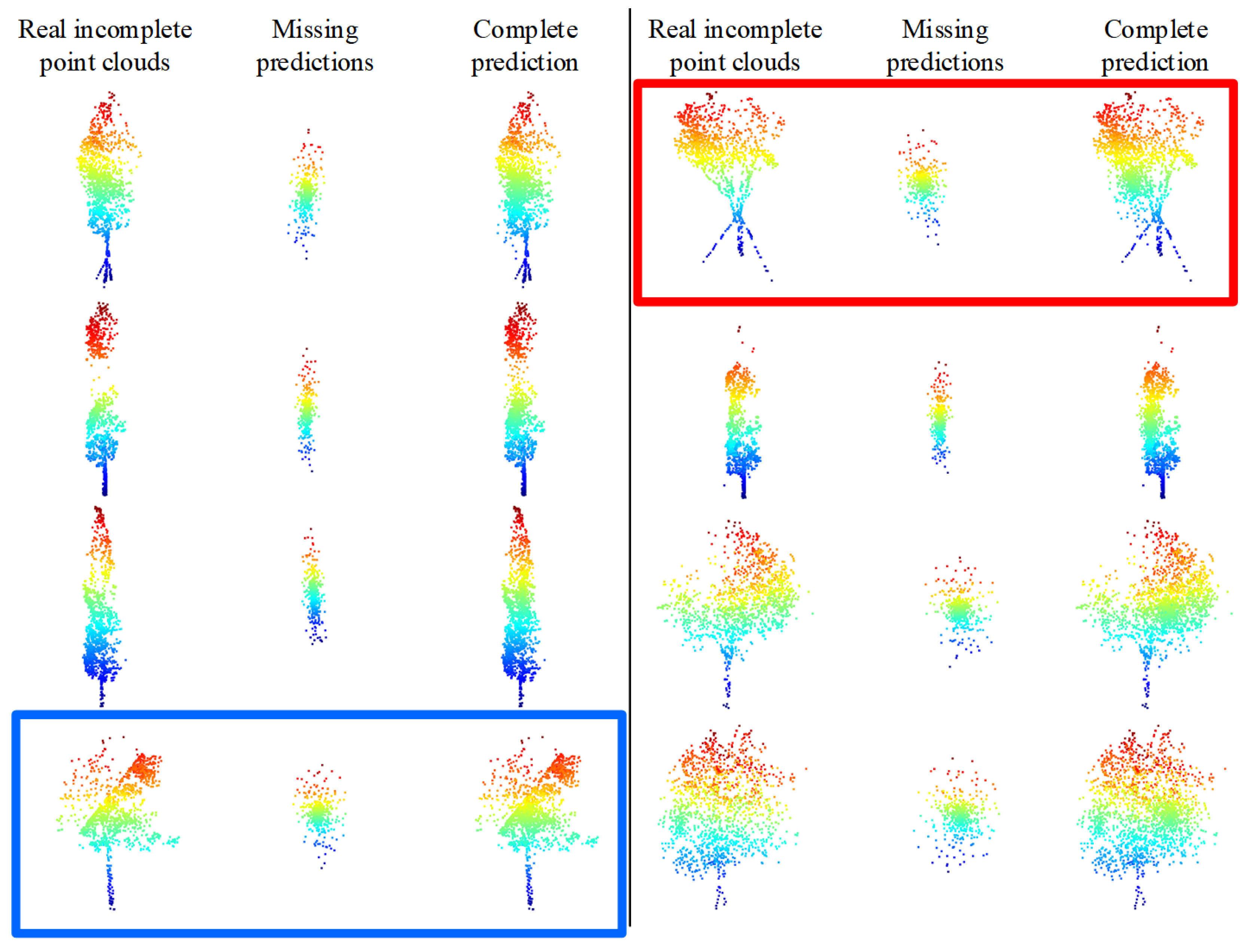
To verify the structure completion effect of the TC-Net model in real scenarios, partial incomplete point clouds that account for the majority of the real scenarios have been selected from the MLS point clouds collected from the test area. We employ the trained model for prediction after directly employing the random sampling to down-sample the incomplete point clouds to 1536 points for each tree, and the predicted results are shown in Figure 14. The model training is based on an uneven density point clouds loss pattern that can effectively discover the missing areas (density reduction areas) and then complete the structure of the real incomplete single tree point clouds. For example, the obvious missing areas of incomplete point clouds, which are marked in the red box in Figure 14, are in the upper right corner. The model correctly predicts and completes structural completion. However, the missing area of the incomplete point clouds marked in the blue box is located in the upper left corner, and the model correctly predicts and completes structural completion.
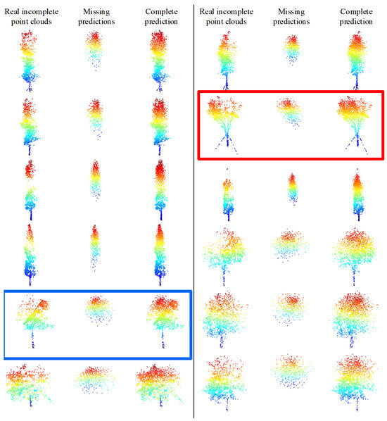
Figure 14.
Model training based on the density loss method directly predicts the true incomplete tree point clouds results. The model correctly predicts and completes the structural completion, as marked by the red and blue boxes.
A comparison is made between the predicted complete single tree point clouds with the UAV airborne oblique photography reconstruction point clouds collected from the same area at the same time. This is to quantitatively analyze whether the direction of the completed structure is consistent with the true missing. The single tree canopy structure in the reconstructed point clouds is more complete owing to the UAV airborne oblique photography method that captures a more comprehensive perspective. The predicted complete single tree point clouds being closer to the reconstructed point clouds than the original incomplete point clouds, that is, the CD value being smaller, will indicate the effective single tree structure completion with TC-Net.
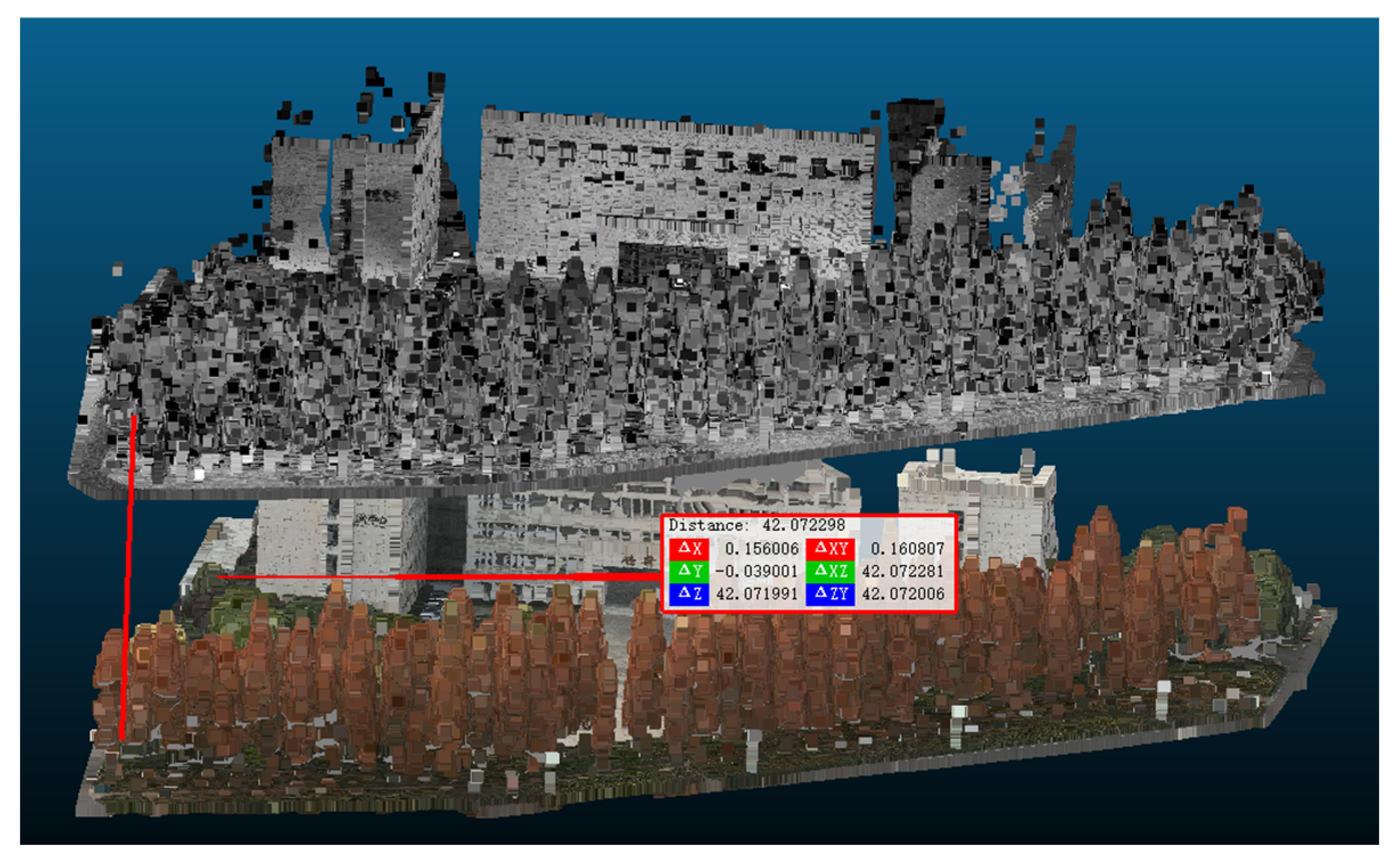
According to Figure 15, the above part is the MLS point clouds, and the below one is the reconstructed point clouds. These parts owe to a certain offset between the reconstructed point clouds and the MLS point clouds; further registration steps are required in the process of quantitatively calculating the right CD value to ensure that the coordinates of the two are aligned, or need to process the registration operation. The specific registration method is described as follows. Owing to both the reconstructed point clouds and the MLS point clouds having GPS information and elevation values, there are basically no scale differences or rotation angle differences, that is, the main registration operations are the horizontal and vertical offsets. Accordingly, we have selected multiple points located on the road and the building corner as homonymous points and performed point registration operations according to the homonymous points.

Figure 15.
Comparison of different types of point clouds in the test area. MLS point clouds is shown above, and the reconstructed point clouds is shown below.
This study has randomly selected certain trees from 3 testing areas to quantitatively demonstrate the single tree completion effect of the TC-Net model. Furthermore, the visualization method proposed in this study has also been utilized to assist in evaluating the completion effect. Further, we have registered their original incomplete point clouds and the structural completion point clouds of the trained TC-Net model, based on an uneven density pattern, with the reconstructed point clouds (as the true value) simultaneously. Then we calculated their CD values according to the corresponding formula (calculation times was 2048 points, where the original incomplete point clouds and the reconstructed point clouds were randomly down-sampled) and calculated the difference between the two. The results are listed in Table 2.
Table 2.
CD values between the incomplete point clouds and the structure completion point clouds with the reconstructed point clouds after registration.
According to Table 2, the following is observed:
- (1)
- The data with the best completion effect have a serial number of 1. The CD value of the incomplete and reconstructed point clouds is 23.89, whereas the CD value of the completed and reconstructed point clouds is 13.08, with an average difference of 10.81. The difference between the completed point clouds and the reconstructed point clouds is miniscule, which indicates a significant improvement in the structural integrity of the completed point clouds.
- (2)
- From the measurement of average CD value, the overall completion effect decreases by more than a factor of 2. Based on the comparison between the completion effect and the actual situation, for incomplete point clouds with more missing points, the completion effect is stark, and vice versa.
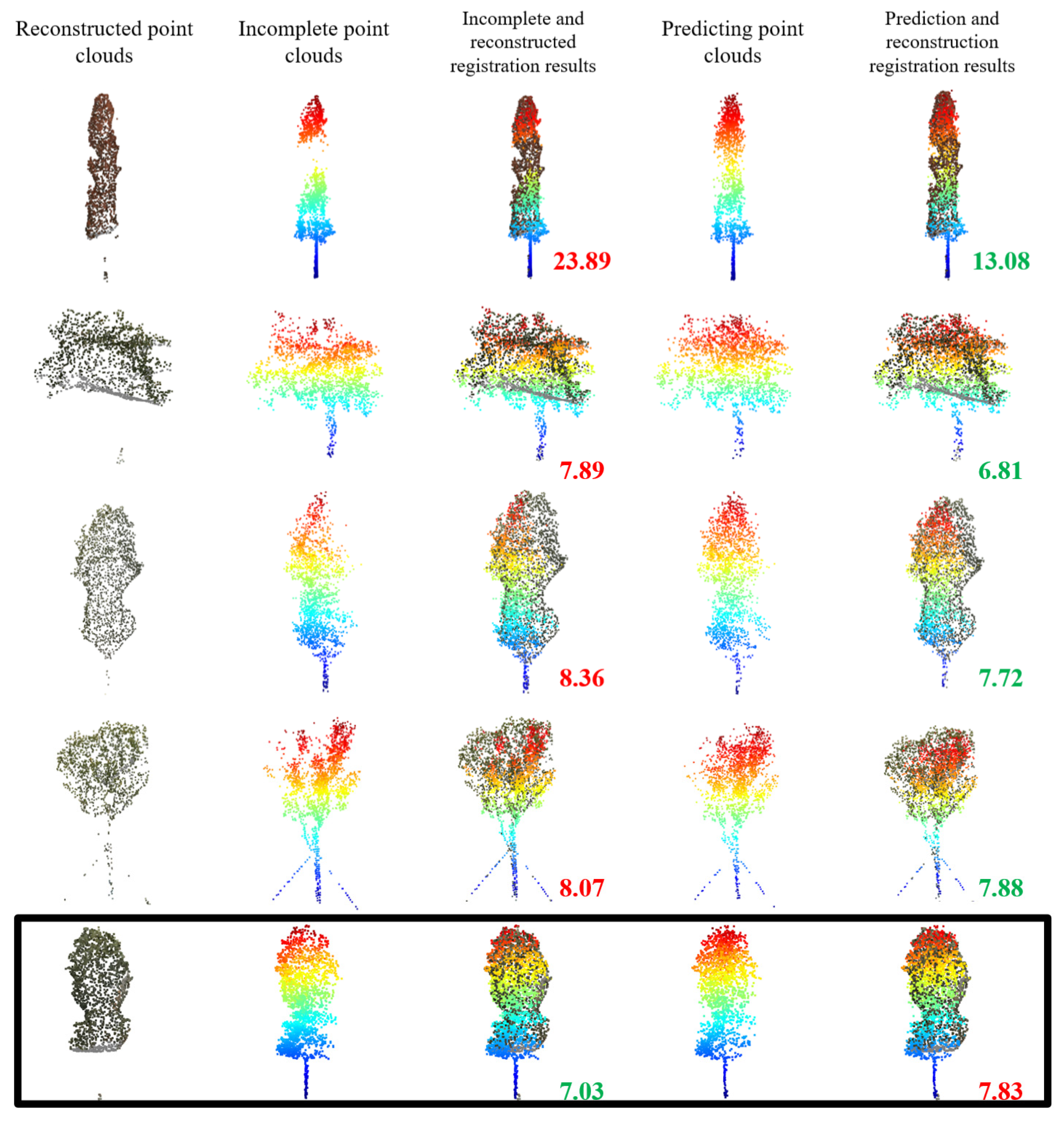
To better illustrate the results, certain visualizations of the results are selected according to Figure 16. The number in the bottom right corner of the registration results is the CD value, and the same row is marked with smaller and larger CD values in green and red colors, respectively. In most cases, the completion of the TC-Net model can make the single tree point cloud canopy results more complete and closer to the reconstructed point clouds. Among them, a few cases occur, as shown in the black box in Figure 16, where the completion increases the CD value primarily owing to the incomplete data missing. However, the increase in CD value is not significant in this case, which implies that the negative effect of the structure completion is not significant. Overall, the completion of the TC-Net model is effective and can make the canopy structure of a single tree point cloud more complete.
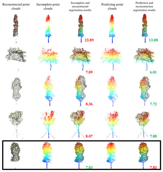
Figure 16.
Comparison of the incomplete point clouds, predicted complete point clouds, and the reconstructed point clouds with different CD values.
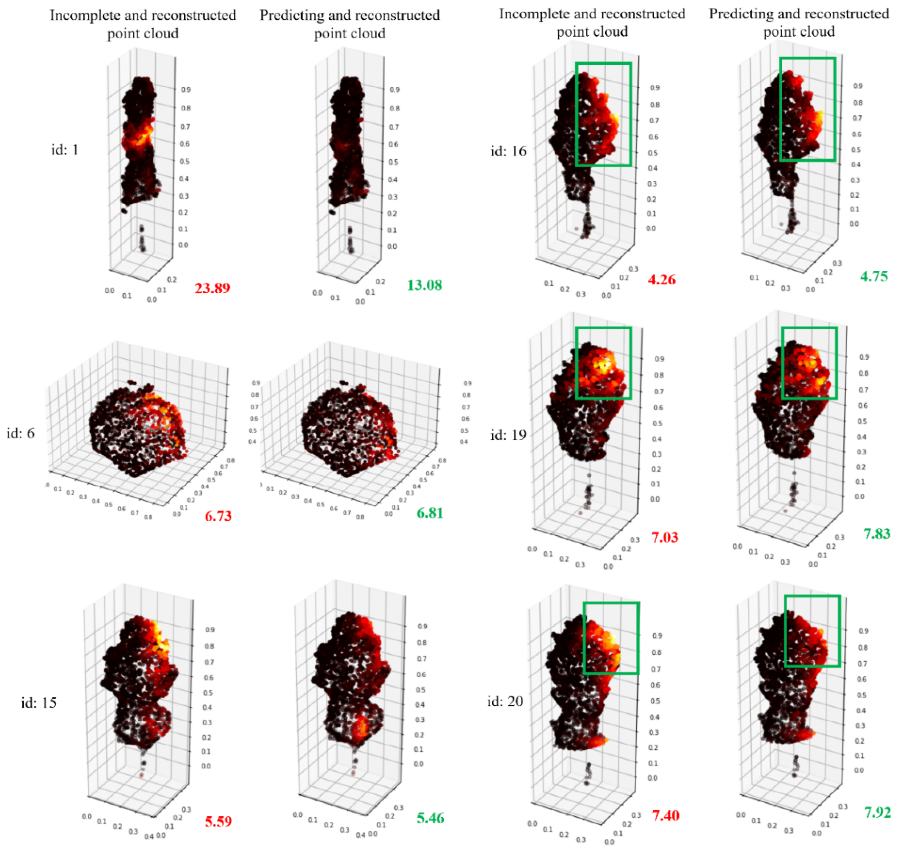
To better demonstrate the completion effect of the method proposed in this study, the local similarity visualization method of point cloud aforementioned will be used to visualize the completion effects of the tree pairs with different CD values, as shown in Table 2. The visual comparison results are shown in Figure 17.
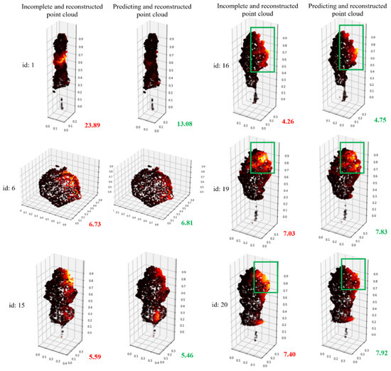
Figure 17.
Visualization comparison of CD values for incomplete and complete point clouds using the local similarity visualization method.
According to Figure 17, tree #1 has the best completion effect, and the missing areas have been well completed. Although the trees #6 and #15 show a change of only 0.1 in CD values, the bright parts have been significantly weakened in the visualization effect. In trees #16, #19, and #20, although the CD value actually becomes larger, the brightness is significantly weakened from the visualization image. This may be due to the non-rigid features of the trees, which leads to some outliers that make the calculation of the CD value abnormal. Therefore, this novel visualization method could better represent the effect of tree point clouds completion than CD values.
4.4. TC-Net Ablation Experiments
In the experiments, the comparisons of the uneven density loss pattern versus the random spherical loss pattern and the pre-trained method versus the non-pre-trained method are carried out in the following.
4.4.1. Uneven Density Loss Pattern vs. Random Spherical Loss Pattern
We attempt a direct training of the TC-Net model using the random spherical loss pattern with the same parameters and data as the training with the uneven density loss pattern. To verify the structure completion effect of the model in real scenarios, partial incomplete point clouds have been selected from the MLS point clouds data, and random sampling is directly employed to down-sample the incomplete point clouds to 1536 points for each single tree. Then, the trained model has been employed for prediction, and the results are demonstrated in Figure 18.
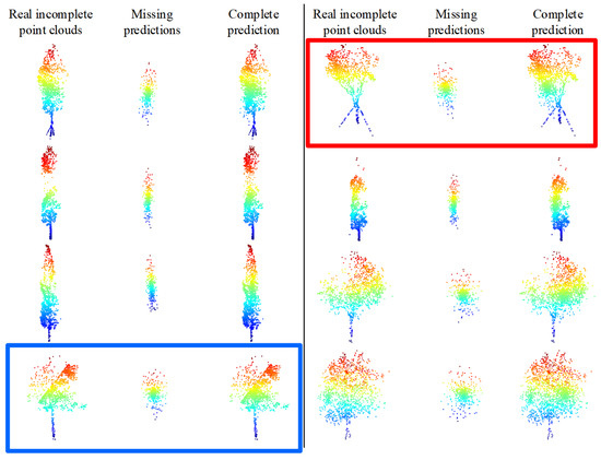
Figure 18.
Direct prediction of real incomplete tree point clouds using a TC-Net trained model based on a random spherical loss pattern.
According to Figure 18, the trained model based on the random spherical loss pattern is completely unable to complete the structure of the real incomplete single tree point clouds. For instance, the incomplete point clouds marked in the red box in Figure 18 are clearly missing in the upper right corner, though the model predicts it in the lower left corner. Whereas, the missing area of the incomplete point clouds labeled in the blue box is in the upper left corner, though the model predicts it in the middle. The other situations are basically similar. Thus the trained models based on this pattern cannot handle the prediction in real situations since the missing pattern of real MLS point clouds data is not a spherical missing, though the uneven density point clouds are caused by limited perspective. As the distance from the vehicle’s driving trajectory increases, the point clouds density will decrease owing to the obstruction of leaves or branches and the limited penetration of LiDAR. Thus, the missing patterns that do not match the real scenarios will result in the loss pattern not being competent for the structure completion smoothly.
4.4.2. Pre-Trained Method vs. Non-Pre-Trained Method
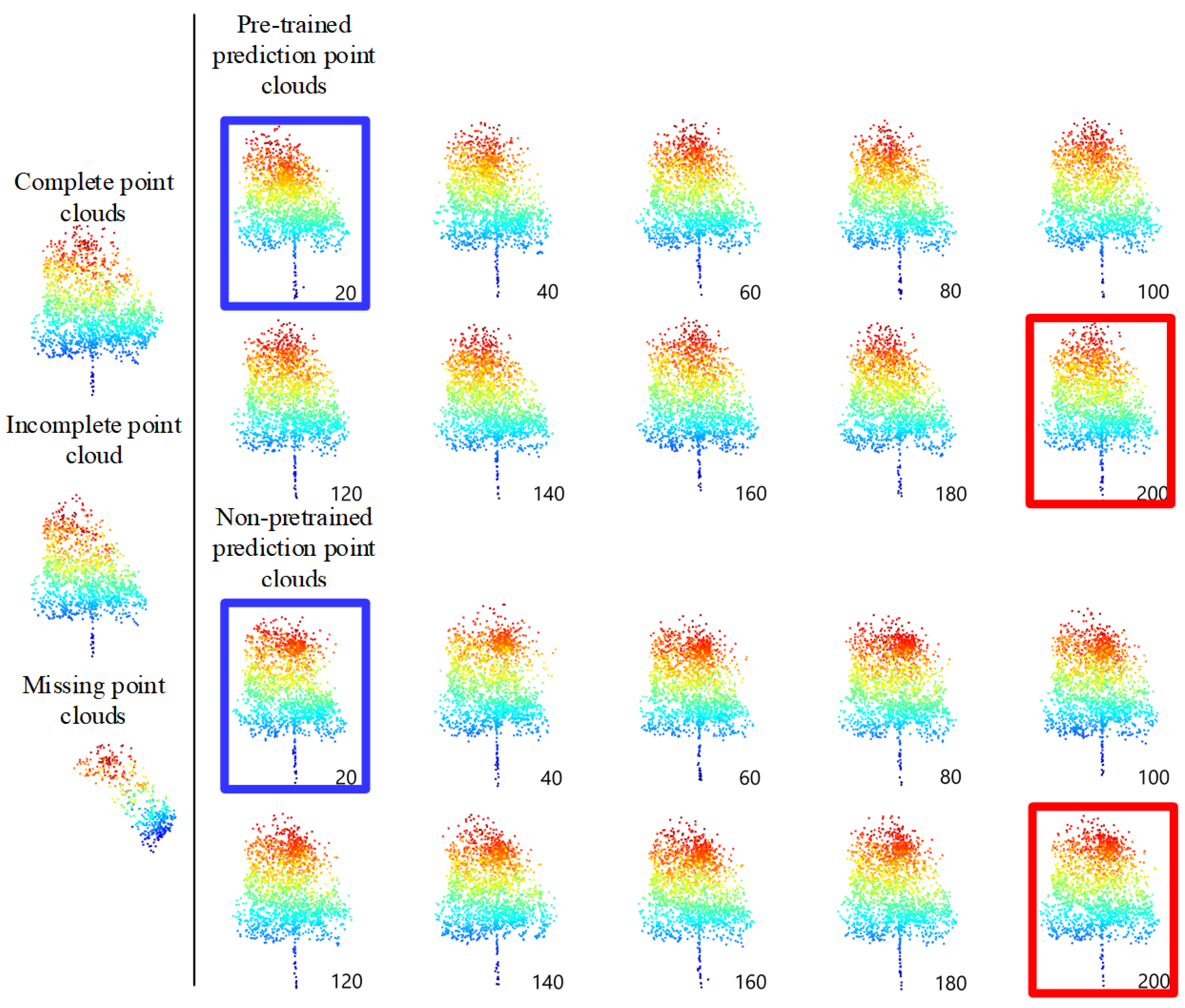
The comparative experiments have been conducted with the same parameters to demonstrate the difference between the pre-trained and non-pre-trained methods. The pre-trained method on 33 single trees point clouds in the testing data set has CD values of 9.20, which is below that of the non-pre-trained method, namely, 9.51. The predicted missing with the pre-trained method is similar to the true missing. Concomitantly, the pre-trained and non-pre-trained models, with an interval of 20 epochs, have been taken to complete the structure completion on the testing data set and to demonstrate the process of the two training methods, and the lane line position is fixed. The completion results are displayed in Figure 19.
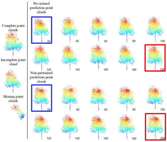
Figure 19.
Comparison results of TC-Net for every 20 epochs between the pre-trained and non-pre-trained methods.
According to Figure 19, the pre-trained model has two main advantages. (1) It performs better in the early stages of training, or can train better and faster, as indicated by the blue box in Figure 19. (2) The final training result is smoother, and there is clustering phenomenon in the predicted areas with the non-pre-trained model, as indicated by the red box in Figure 19.
4.5. Model Comparison Experiments on Our Self-Collected Dataset
Since our method is the pioneer and novel deep-learning-based vegetation completion methods, there are no open-source baselines available at this stage. Existing models primarily focus on the point clouds completion of ordinary objects, thus making it difficult to directly apply them for the vegetation point clouds completion. Thus, to prove the effectiveness of TC-Net, we have taken several state-of-the-art baselines that focus on the point clouds completion of ordinary objects. The selected baselines include TopNet [18] and PMP-Net++ [20]. All networks are retrained on the dataset made by our uneven density loss pattern.
The evaluation metric used in the experiment is also the CD value. After the model has converged, we test it using our self-collected dataset’s test set, and the results are shown in Table 3.
Table 3.
The results of different models on the self-collected dataset.
From Table 3, it found the following data:
- (1)
- The state-of-the-art PMP-Net++, which treats the point clouds completion task as a deformation task, proves effective for regular objects (such as those in the ShapeNet dataset). However, the point cloud data collected by MLS has the characteristic of the dense points near the sensor, whereas the sparse points farther away lead to a lack of effective constraints on the deformation process. From Table 3, it can be seen that after completing the trees, the CD value of our method is 0.28 less than PMP-Net++. As noted in [20], “In all, the research of PMP-Net++ is somewhat limited by the lack of effective constraints to the deformation process.” Therefore, PMP-Net++ does not perform as well as our TC-Net in terms of CD value on the test set.
- (2)
- Similarly, owing to the dense-near and sparse-far characteristics of MLS point clouds and the irregular shape of trees, TopNet, which is sensitive to input data volume, also performs worse than TC-Net in the self-collected tree completion tasks. From Table 3, it can be seen that after completing the trees, the CD value of our method is 0.57 less than TopNet.
4.6. Model Comparison Experiments on Large-Scale Tree Dataset
Due to limited conditions, the self-collected tree dataset only contains a few hundred to thousands of trees. In order to further validate the effectiveness of TC-Net on large datasets, experiments were conducted on a comprehensive large-scale 3D synthetic tree dataset, TreeNet3D [39].
The TreeNet3D dataset includes 10 species of trees, totaling 13,834 simulated trees. We allocated 11,000 trees for training and 2834 for testing. During the training, we processed each tree using the proposed uneven density loss pattern and input them into the network for training. After the network converged, we conducted experiments on the test set. The results are shown in Table 4.
Table 4.
The results of different models on TreeNet3D.
As shown in Table 4, compared with TopNet and PMP-Net++, TC-Net performs well on the simulated dataset, with the lowest average CD value of 13.28, demonstrating high accuracy and consistency across various types of data. Additionally, TC-Net performs well on most specific tree species, indicating its robustness.
4.7. Practical Application Verification Experiment of the TC-Net Model
TC-Net can be employed to complete the missing individual trees in the project of urban area LVV calculation, thereby making the 3D green quantity data more accurate. In the project, the complete automation LVV calculation scheme for urban areas is displayed in Figure 20.
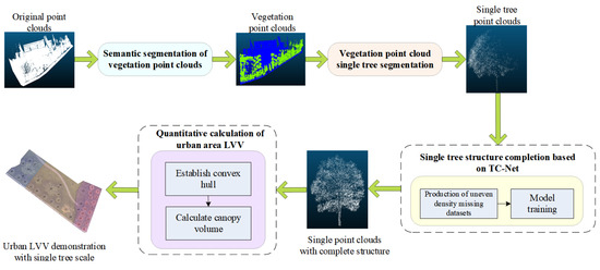
Figure 20.
Automated LVV calculation scheme in urban areas.
According to Figure 20, the urban area LVV calculation mainly includes the following, namely, (1) semantic segmentation of the original point clouds to extract vegetation information from complex terrain and (2) performing single tree segmentation on the extracted vegetation point clouds to obtain a single tree scale point cloud. (3) Based on TC-Net, the complete structure of a single tree point clouds to obtain a complete single tree point cloud, and (4) calculating the LVV of a single tree in an urban area based on the convex hull model.
TA #1 has been selected for this experiment, as shown in Figure 10, as the comprehensive verification site. The measurement area has typical low and tall roadside trees along bidirectional roads. The vegetation point clouds in the measurement area have been obtained through MLS, which shows typical point clouds missing phenomena, thus meeting the verification requirements of this experiment.
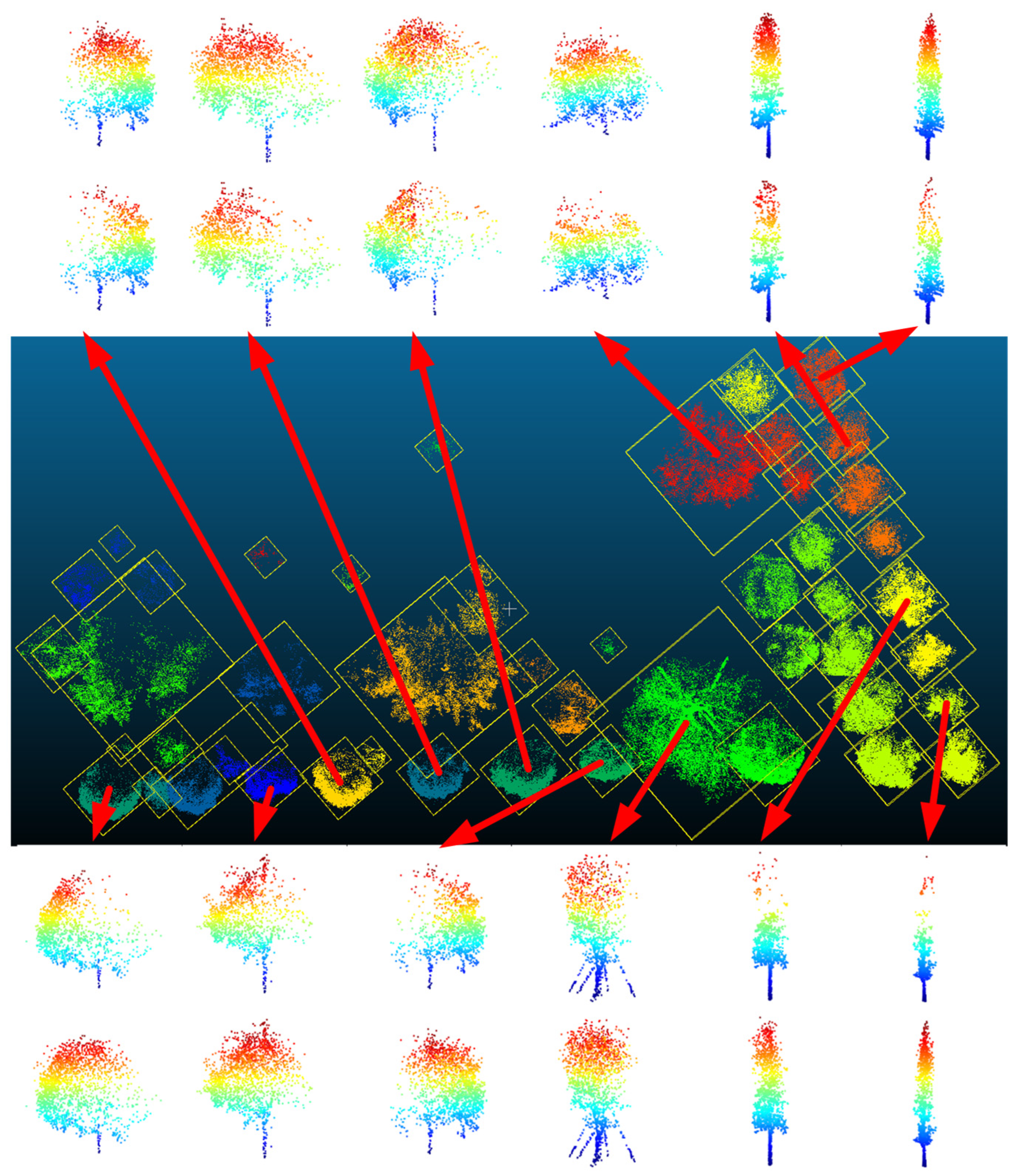
According to the abovementioned LVV automation calculation scheme, this study first performs semantic segmentation based on the HPCT (hierarchical point clouds transformer) [37] model on the point clouds data of TA #1 and extracts the vegetation point clouds in the measurement area. Next, a hybrid clustering method (combining K-Means and DBSCAN) is employed to achieve single tree segmentation of the vegetation point clouds, thus resulting in incomplete single tree point clouds. The results of the single tree segmentation in TA #1 are shown in Figure 21, with each box representing single tree point clouds.
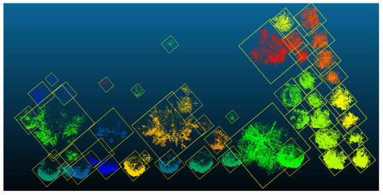
Figure 21.
Experimental results of single tree segmentation from vegetation point clouds.
Subsequently, a single tree point cloud has been randomly down-sampled as the input, and the complete structure of the single tree point clouds is obtained through TC-Net prediction, as displayed in Figure 22. According to certain selected results for visualization (the top and bottom rows correspond to the completion effect of individual trees), the TC-Net mode can effectively identify the missing patterns and complete the structural completion, thereby improving the accuracy of subsequent LVV calculations.
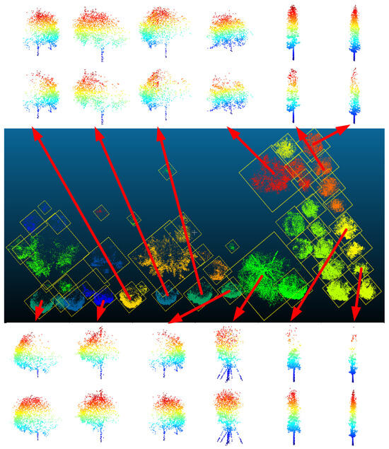
Figure 22.
Completion results of single tree structure based on TC-Net in TA #1.
Therefore, this study establishes the convex hull of a single tree point clouds based on the Graham-Scan algorithm and employs the mixed product formula to calculate the volume of the convex hull to represent the LVV of a single tree. Particularly, the canopy volume has been chosen to represent LVV. The incomplete single tree point clouds and the non-canopy part of the single tree structure completion results (both of which are 2048 points) mentioned earlier have been removed from the main trunk, and only the canopy is retained. Then, the convex hulls have been established to calculate the volume and obtain the LVV value corresponding to the single tree scale.
To illustrate the effect of a single tree structure completion on improving the accuracy of LVV calculation, this study calculates the true value of LVV based on the formula method [1] and compares it with the calculated LVV values based on complete point clouds and incomplete point clouds, as shown in Table 5. The calculated LVV values of the complete point clouds are closer to the true value, that is, the single tree structure completion can effectively improve the accuracy of LVV calculation.
Table 5.
LVV values based on convex hull calculation and the true values of LVV calculated by the formula method, in m3.
We calculate the mean absolute error (MAE), mean square error (MSE), and mean absolute percentage error (MAPE) of the LVV values and true values, prior and post the completion for the trees in Table 5. The completed trees have smaller errors while calculating the LVV, that is, the average MAE, RSME, and MAPE of the LVV values have decreased from 9.57, 7.78, and 14.11% to 1.86, 2.84, and 5.23%, respectively. This is with respect to the LVV calculation from the incomplete and completed point clouds.
Finally, by employing the LVV results, a corresponding thematic map of the survey area can be created.
5. Conclusions
The mutual occlusion between the ground objects and the limitation of sensor perspective and penetration ability lead to the lack of single tree point cloud structure and the uneven point cloud density (i.e., the dense points near the sensor whereas the sparse points farther away the sensor). The commonly employed methods in forestry remote sensing have limitations in experimental conditions and cannot achieve accurate completion. This study introduces a data-driven, self-supervised point clouds structural completion method, that is, the proposed TC-Net model and the corresponding uneven density point clouds loss pattern. To evaluate the approach, a complete single tree dataset for this field has been constructed from our self-collected MLS point clouds data. Finally, it has been experimentally proven that the approach can accurately compensate for the single tree structure. Further, it can be applied in the field of vegetation point clouds processing and analysis, such as the urban area LVV calculation.
Furthermore, we can investigate from the following directions:
- (1)
- Complete the variable density single tree structure. Increasing the density of a single tree point clouds can provide more geometric details. We can attempt the density improvement method in PMP-Net++ [20], which involves the random sampling of the same incomplete single tree point clouds multiple times, inputting the sampling results into the structural completion model for completion, and then overlaying the completion results for obtaining a predicted higher density point clouds.
- (2)
- Completing the single tree structure from multiple sources. We can register the completed MLS point clouds of the same single tree with other point clouds data sources, such as the UAV airborne LiDAR point clouds and UAV airborne oblique photogrammetric reconstruction point clouds, to construct the complete (incomplete) tree pairs for training the structural completion model, that is, TC-Net. This can be employed to complete the structure for multi-source point clouds.
Author Contributions
F.H.: conceptualization, resources, supervision, funding acquisition. B.G.: conceptualization, methodology, software, writing. S.C.: software, validation, writing. W.H.: data curation, writing. X.Q.: data curation, writing. J.L.: conceptualization, review. G.T.: conceptualization, review. All authors have read and agreed to the published version of the manuscript.
Funding
This research was funded by the National Natural Science Foundation of China, Project No. 42271390.
Data Availability Statement
The data supporting this study’s findings are available at https://github.com/fhuang80/TC-Net (accessed on 1 September 2024).
Conflicts of Interest
The authors declare no conflicts of interest.
References
- Huang, F.; Peng, S.; Chen, S.; Cao, H.; Ma, N. VO-LVV—A Novel Urban Regional Living Vegetation Volume Quantitative Estimation Model Based on the Voxel Measurement Method and an Octree Data Structure. Remote Sens. 2022, 14, 855. [Google Scholar] [CrossRef]
- Huang, Z.; Yu, Y.; Xu, J.; Ni, F.; Le, X. PF-Net: Point Fractal Network for 3D Point Cloud Completion. In Proceedings of the 2020 IEEE/CVF Conference on Computer Vision and Pattern Recognition (CVPR), Seattle, WA, USA, 13–19 June 2020; pp. 7659–7667. [Google Scholar] [CrossRef]
- Sarkar, K.; Varanasi, K.; Stricker, D. Learning Quadrangulated Patches for 3D Shape Parameterization and Completion. In Proceedings of the 2017 International Conference on 3D Vision (3DV), Qingdao, China, 10–12 October 2017; pp. 383–392. [Google Scholar] [CrossRef]
- Sung, M.; Kim, V.G.; Angst, R.; Guibas, L. Data-driven structural priors for shape completion. ACM Trans. Graph. 2015, 34, 1–11. [Google Scholar] [CrossRef]
- Li, Y.; Dai, A.; Guibas, L.; Nießner, M. Database-Assisted Object Retrieval for Real-Time 3D Reconstruction. Comput. Graph. Forum 2015, 34, 435–446. [Google Scholar] [CrossRef]
- Martinovic, A.; Van Gool, L. Bayesian Grammar Learning for Inverse Procedural Modeling. In Proceedings of the 2013 IEEE Conference on Computer Vision and Pattern Recognition (CVPR), Portland, OR, USA, 23–28 June 2013; pp. 201–208. [Google Scholar] [CrossRef]
- Rock, J.; Gupta, T.; Thorsen, J.; Gwak, J.; Shin, D.; Hoiem, D. Completing 3D object shape from one depth image. In Proceedings of the 2015 IEEE Conference on Computer Vision and Pattern Recognition (CVPR), Boston, MA, USA, 7–12 June 2015; pp. 2484–2493. [Google Scholar] [CrossRef]
- Mitra, N.J.; Pauly, M.; Wand, M.; Ceylan, D. Symmetry in 3D Geometry: Extraction and Applications. Comput. Graph. Forum 2013, 32, 1–23. [Google Scholar] [CrossRef]
- Qi, Y.; Coops, N.C.; Daniels, L.D.; Butson, C.R. Comparing tree attributes derived from quantitative structure models based on drone and mobile laser scanning point clouds across varying canopy cover conditions. ISPRS J. Photogramm. Remote Sens. 2022, 192, 49–65. [Google Scholar] [CrossRef]
- Xu, H.; Gossett, N.; Chen, B. Knowledge and heuristic-based modeling of laser-scanned trees. ACM Trans. Graph. 2007, 26, 19. [Google Scholar] [CrossRef]
- Zhang, X.; Li, H.; Dai, M.; Ma, W.; Quan, L. Data-Driven Synthetic Modeling of Trees. IEEE Trans. Vis. Comput. Graph. 2014, 20, 1214–1226. [Google Scholar] [CrossRef] [PubMed]
- Mei, J.; Zhang, L.; Wu, S.; Wang, Z.; Zhang, L. 3D tree modeling from incomplete point clouds via optimization and L 1-MST. Int. J. Geogr. Inf. Sci. 2017, 31, 999–1021. [Google Scholar] [CrossRef]
- Cao, W.; Wu, J.; Shi, Y.; Chen, D. Restoration of Individual Tree Missing Point Cloud Based on Local Features of Point Cloud. Remote Sens. 2022, 14, 1346. [Google Scholar] [CrossRef]
- Achlioptas, P.; Diamanti, O.; Mitliagkas, I.; Guibas, L. Learning Representations and Generative Models for 3D Point Clouds. In Proceedings of the 35th International Conference on Machine Learning (ICML), Stockholm, Sweden, 10–15 July 2018; pp. 40–49. [Google Scholar]
- Yang, Y.; Feng, C.; Shen, Y.; Tian, D. FoldingNet: Point Cloud Auto-Encoder via Deep Grid Deformation. In Proceedings of the 2018 IEEE/CVF Conference on Computer Vision and Pattern Recognition (CVPR), Salt Lake City, UT, USA, 18–23 June 2018; pp. 206–215. [Google Scholar] [CrossRef]
- Yuan, W.; Khot, T.; Held, D.; Mertz, C.; Hebert, M. PCN: Point Completion Network. In Proceedings of the 2018 International Conference on 3D Vision (3DV), Verona, Italy, 5–8 September 2018; pp. 728–737. [Google Scholar] [CrossRef]
- Sarmad, M.; Lee, H.J.; Kim, Y.M. RL-GAN-Net: A Reinforcement Learning Agent Controlled GAN Network for Real-Time Point Cloud Shape Completion. In Proceedings of the 2019 IEEE/CVF Conference on Computer Vision and Pattern Recognition (CVPR), Long Beach, CA, USA, 15–20 June 2019; pp. 5891–5900. [Google Scholar] [CrossRef]
- Tchapmi, L.P.; Kosaraju, V.; Rezatofighi, H.; Reid, I.; Savarese, S. TopNet: Structural Point Cloud Decoder. In Proceedings of the 2019 IEEE/CVF Conference on Computer Vision and Pattern Recognition (CVPR), Long Beach, CA, USA, 15–20 June 2019; pp. 383–392. [Google Scholar] [CrossRef]
- Cheng, M.; Li, G.; Chen, Y.; Chen, J.; Wang, C.; Li, J. Dense Point Cloud Completion Based on Generative Adversarial Network. IEEE Trans. Geosci. Remote Sens. 2021, 60, 1–10. [Google Scholar] [CrossRef]
- Wen, X.; Xiang, P.; Han, Z.; Cao, Y.-P.; Wan, P.; Zheng, W.; Liu, Y.-S. PMP-Net++: Point Cloud Completion by Transformer-Enhanced Multi-Step Point Moving Paths. IEEE Trans. Pattern Anal. Mach. Intell. 2022, 45, 852–867. [Google Scholar] [CrossRef] [PubMed]
- Fei, B.; Yang, W.; Chen, W.-M.; Li, Z.; Li, Y.; Ma, T.; Hu, X.; Ma, L. Comprehensive Review of Deep Learning-Based 3D Point Cloud Completion Processing and Analysis. IEEE Trans. Intell. Transp. Syst. 2022, 23, 22862–22883. [Google Scholar] [CrossRef]
- Ibrahim, Y.; Nagy, B.; Benedek, C. Multi-view Based 3D Point Cloud Completion Algorithm for Vehicles. In Proceedings of the 2022 26th International Conference on Pattern Recognition (ICPR), Montreal, QC, Canada, 21–25 August 2022; pp. 2121–2127. [Google Scholar]
- Toscano, J.D.; Zuniga-Navarrete, C.; Siu, W.D.J.; Segura, L.J.; Sun, H. Teeth Mold Point Cloud Completion Via Data Augmentation and Hybrid RL-GAN. J. Comput. Inf. Sci. Eng. 2023, 23, 041008. [Google Scholar] [CrossRef]
- Sipiran, I.; Mendoza, A.; Apaza, A.; Lopez, C. Data-Driven Restoration of Digital Archaeological Pottery with Point Cloud Analysis. Int. J. Comput. Vis. 2022, 130, 2149–2165. [Google Scholar] [CrossRef]
- Singer, N.; Asari, V.K. View-Agnostic Point Cloud Generation for Occlusion Reduction in Aerial Lidar. Remote Sens. 2022, 14, 2955. [Google Scholar] [CrossRef]
- Li, X.; Zhou, Z.; Xu, Z.; Jiang, H.; Zhao, H. Plant Leaf Point Cloud Completion based on Deep Learning. In Proceedings of the Sixth Symposium on Novel Optoelectronic Detection Technology and Applications, Beijing, China, 3–5 December 2019; Volume 11455, pp. 1879–1883. [Google Scholar]
- Xiao, H.; Xu, H.; Ma, S. Point Cloud Complementation Method of Epipremnum aureum Leaves under Occlusion Conditions Based on MSF-PPD Network. Trans. Chin. Soc. Agric. Mach. 2021, 52, 141–148. [Google Scholar]
- Jiang, J.; Li, L.; Wang, M. Research on plant stem complement based on L1-medial skeleton extraction. J. Nanjing For. Univ. 2022, 46, 40–50. [Google Scholar]
- Cai, S.; Zhang, W.; Zhang, S.; Yu, S.; Liang, X. Branch architecture quantification of large-scale coniferous forest plots using UAV-LiDAR data. Remote Sens. Environ. 2024, 306, 114121. [Google Scholar] [CrossRef]
- Pan, L.; Liu, L.; Condon, A.G.; Estavillo, G.M.; Coe, R.A.; Bull, G.; Stone, E.A.; Petersson, L.; Rolland, V. Biomass Prediction with 3D Point Clouds from LiDAR. In Proceedings of the 2022 IEEE/CVF Winter Conference on Applications of Computer Vision (WACV), Waikoloa, HI, USA, 3–8 January 2022; pp. 1716–1726. [Google Scholar] [CrossRef]
- Xu, D.; Chen, G.; Jing, W. A Single-Tree Point Cloud Completion Approach of Feature Fusion for Agricultural Robots. Electronics 2023, 12, 1296. [Google Scholar] [CrossRef]
- Qi, C.R.; Yi, L.; Su, H.; Guibas, L.J. PointNet++: Deep Hierarchical Feature Learning on Point Sets in a Metric Space. In Proceedings of the Advances in Neural Information Processing Systems, Long Beach, CA, USA, 4–9 December 2017; pp. 1–10. [Google Scholar]
- Guo, M.-H.; Cai, J.-X.; Liu, Z.-N.; Mu, T.-J.; Martin, R.R.; Hu, S.-M. PCT: Point cloud transformer. Comput. Vis. Media 2021, 7, 187–199. [Google Scholar] [CrossRef]
- Chang, A.X.; Funkhouser, T.; Guibas, L.; Hanrahan, P.; Huang, Q.; Li, Z.; Savarese, S.; Savva, M.; Song, S.; Su, H.; et al. Shapenet: An information-rich 3d model repository. arXiv 2015, arXiv:1512.03012. [Google Scholar]
- Bleaney, B. Electricity and Magnetism; Oxford University Press: Oxford, UK, 2013; Volume 2. [Google Scholar]
- Paszke, A. PyTorch: An Imperative Style, High-Performance Deep Learning Library. In Proceedings of the Advances in Neural Information Processing Systems 32 (NeurIPS 2019), Vancouver, BC, Canada, 8–14 December 2019; pp. 8026–8037. [Google Scholar]
- Qiang, X.; He, W.; Chen, S.; Lv, Q.; Huang, F. Hierarchical point cloud transformer: A unified vegetation semantic segmentation model for multisource point clouds based on deep learning. IEEE Trans. Geosci. Remote Sens. 2023, 61, 1–16. [Google Scholar] [CrossRef]
- Yi, L.; Kim, V.G.; Ceylan, D.; Shen, I.-C.; Yan, M.; Su, H.; Lu, C.; Huang, Q.; Sheffer, A.; Guibas, L. A scalable active framework for region annotation in 3D shape collections. ACM Trans. Graph. 2016, 35, 1–12. [Google Scholar] [CrossRef]
- Tang, S.; Ao, Z.; Li, Y.; Huang, H.; Xie, L.; Wang, R.; Wang, W.; Guo, R. TreeNet3D: A large scale tree benchmark for 3D tree modeling, carbon storage estimation and tree segmentation. Int. J. Appl. Earth Obs. Geoinf. 2024, 130, 103903. [Google Scholar] [CrossRef]


Disclaimer/Publisher’s Note: The statements, opinions and data contained in all publications are solely those of the individual author(s) and contributor(s) and not of MDPI and/or the editor(s). MDPI and/or the editor(s) disclaim responsibility for any injury to people or property resulting from any ideas, methods, instructions or products referred to in the content. |
© 2024 by the authors. Licensee MDPI, Basel, Switzerland. This article is an open access article distributed under the terms and conditions of the Creative Commons Attribution (CC BY) license (https://creativecommons.org/licenses/by/4.0/).