Article

FE-SKViT: A Feature-Enhanced ViT Model with Skip Attention for Automatic Modulation Recognition

1
School of Electronic Engineering, Xidian University, Xi’an 710071, China
2
China Xi’an Satellite Control Center, Xi’an 710043, China
*
Author to whom correspondence should be addressed.
Remote Sens. 2024, 16(22), 4204; https://doi.org/10.3390/rs16224204
Submission received: 8 October 2024 / Revised: 28 October 2024 / Accepted: 7 November 2024 / Published: 11 November 2024

Abstract

:
Automatic modulation recognition (AMR) is widely employed in communication systems. However, under conditions of low signal-to-noise ratio (SNR), recent studies reveal limitations in achieving high AMR accuracy. In this work, we introduce a novel network architecture that leverages a transformer-inspired approach tailored for AMR, called Feature-Enhanced Transformer with skip-attention (FE-SKViT). This innovative design adeptly harnesses the advantages of translation variant convolution and the Transformer framework, handling intra-signal variance and small cross-signal variance to achieve enhanced recognition accuracy. Experimental results on RadioML2016.10a, RadioML2016.10b, and RML22 datasets demonstrate that the Feature-Enhanced Transformer with skip-attention (FE-SKViT) excels over other methods, particularly under low SNR conditions ranging from −4 to 6 dB.

1. Introduction

The rapid evolution of deep learning (DL) [1,2] techniques has significantly impacted various fields, including image processing, natural language processing, and speech recognition, acting as an intermediary between signal detection and demodulation. AMR [3,4] significantly facilitates the efficient classification of the modulation types [5]. AMR methods can be categorized into likelihood-based (LB) [6], feature-based (FB) [7], and deep learning (DL) [8,9]. DL-based methods in AMR leverage advanced learning paradigms to enhance model performance and adaptability.
DL-based AMR methods typically involves two consecutive stages. In the initial stage, preprocessing is applied to the received signal to ensure its appropriate representation for subsequent utilization. In the following stage, deep neural networks (DNNs) [10] are employed to process the signal representations and determine the modulation scheme.
In the preprocessing stage, the signal is mainly transformed into four representations, including image representation [11], feature representation [12], sequence representation [13], and combined representation [14]. For each representation, the received signal has been represented in various formats.
The idea of image representation is to transform the received signal into images, such as Constellation Diagram [15], Eye Diagram [16], Bispectrum Gragh [17], and Spectral Correlation Function Image [18], with which the task of modulation classification is performed via image recognition. However, this approach does come with a few limitations: (1) transforming signals into images increases the algorithm’s complexity and (2) to ensure high recognition rates, there are strict requirements on the size of the transformed images, which can impact the model’s real-time inference performance.
The purpose of feature representation is to extract a set of features that accurately characterize the received signal. Importantly, the number of extracted features is typically less than the length of the received signal, facilitating simpler DNNs with reduced complexity in neurons and layers. However, it is worth noting that calculating signal features also adds to the computational complexity.
Currently, research mainly focuses on image and feature representations, as they effectively use established deep learning techniques. Researchers are exploring the optimization of these representations for various modulation schemes.
In the second stage, we categorize these DL-based AMR methods into CNN-based [19], RNN-based [20], GRU-based [21], LSTM-based [22], and transformer-based [23] methods. Transformers utilize multi-head self-attention mechanisms to model contextual information in signals, which is particularly suitable for the sequential nature of signal data. Consequently, recent papers have endeavored to make improvements based on ViT, designing preprocessing methods tailored for IQ signals before feeding them into ViT for recognition, achieving satisfactory outcomes.
In the domain of AMR, an innovative approach was presented by the authors in [24], integrating a frame-wise embedding module (FEM) into a transformer-based architecture to capture global signal characteristics. Unlike conventional Vision Transformer (ViT) [25] models, which rely on fixed-sized patches, the FEM aggregates multiple signal samples into single tokens in the embedding stage, facilitating a more efficient token sequence. This process enables the transformer to extract global features across the entire signal while mitigating locality bias. By removing reliance on convolutional or recurrent layers, the FEM fully activates the parallelism advantages of the transformer, resulting in improved classification accuracy and reduced computation time. This novel structure optimizes the token sequence generation process, making the model more suitable for AMR tasks.
Another significant contribution is noted in [26], where the authors proposed a vision-inspired transformer model to effectively tackle the challenge of feature extraction from signals. One kernel block possess a fundamental trait known as translation equivariance [27], which involves the spatial sharing of filters in a sliding window manner. While this approach reduces the number of parameters, it limits its ability to adapt to various positions within a signal. Consequently, their model incorporates a multi-kernel block, enabling it to perceive signals with varying kernel sizes, thus facilitating both fine-grained and broad-scoped feature capture.
Furthermore, in [28], the authors introduced a novel relative position embedding technique within the Complex-Valued Transformer (CV-TRN) framework for AMR. This method emphasizes relationships between symbols based on their relative positioning, which is crucial for enhancing automatic modulation recognition (AMR) performance. Through meticulous experimentation on frame length L and step size R during the frame-wise embedding process, they investigated how these hyper-parameters specifically influence improvements in AMR system capabilities.
It can be concluded that the crucial aspect of DL-based AMR lies in effectively enhancing feature expression capabilities in low SNR conditions, constraining the improvement of related model performance. To improve this issue, our contributions are summarized as follows:
  • A comprehensive analysis of feature enhancement (FE) improves the effectiveness of feature extraction from input signals;
  • A high-accuracy network based on ViT with FE and skip attention (SKAT), named (FE-SKViT), is proposed for automatic modulation classification;
  • Compared to mainstream DL methods, the proposed FE-SKViT can achieve effective and robust modulation classification performance.
The rest of this paper is organized as follows. Section 2 provides an overview of the signal model. Section 3 describes the FE-SKViT model in detail. Section 4 presents some experimental results from various perspectives. Section 5 gives the conclusions.

2. An Overview of Signal Model

In digital communication systems, the received signal r ( t ) is typically modeled to account for various distortions and noise introduced during transmission. The received signal r ( t ) can be expressed as:
r ( t ) = s ( t ) h ( t ) + n ( t )
where s ( t ) represents the transmitted RF signal, ∗ denotes the convolution operation, h ( t ) denotes the channel impulse response, and n ( t ) represents additive white Gaussian noise (AWGN).
For M-ary Continuous Phase Frequency Shift Keying (CPFSK) signals, as illustrated in Figure 1, the transmitted signal s ( t ) can be defined as:
s ( t ) = cos 2 π f c t + 2 π h t m ( τ ) d τ + ϕ 0
m ( t ) = n = d n g ( t n T s )
where f c is the carrier frequency, h is the modulation index, m ( t ) is typically a sequence of impulses modulated by the data symbols d n , and ϕ 0 is the initial phase.
For CPFSK, the pulse shaping function g ( t ) is usually a rectangular pulse given by:
g ( t ) = 1 if 0 t < T s 0 otherwise
where T s is the symbol period and g ( t ) is the pulse shaping function.
Then, the received signal r ( t ) is quadrature sampled at the receiver to obtain the in-phase (I) and quadrature (Q) components, which can be represented as:
r ( n ) = ( r 1 I , r 1 Q ) , ( r 2 I , r 2 Q ) , , ( r N I , r N Q )
where N denotes the sampling length.

3. Proposed Method

3.1. Overall Architecture

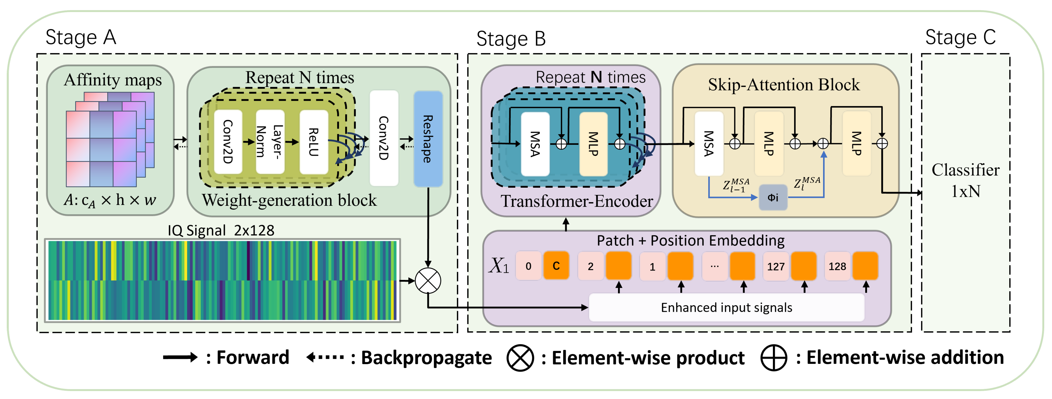
The detailed architecture of FE-SKViT is illustrated in Figure 2, conforming to the procedure as follows.
In our research involving software-defined radio (SDR) platforms, we encountered the inevitable presence of noise in the recorded IQ data, which poses a significant challenge to deep learning classification models prone to overfitting. To address this, we harnessed the concept of TVConv [29], leveraging its ability to capture layout-specific features, to effectively attenuate noise in the frequency domain. By these findings, we introduced a novel model termed FE-SKViT, which incorporates a feature enhancement block to suppress noise in the frequency domain, coupled with ViT’s multi-head self-attention mechanism and the SKAT [30] framework, as illustrated in Figure 3, for efficient and in-depth feature extraction.

3.2. Investigation on the AMC with Distribution of Cross-Signal and Intra-Signal Variance

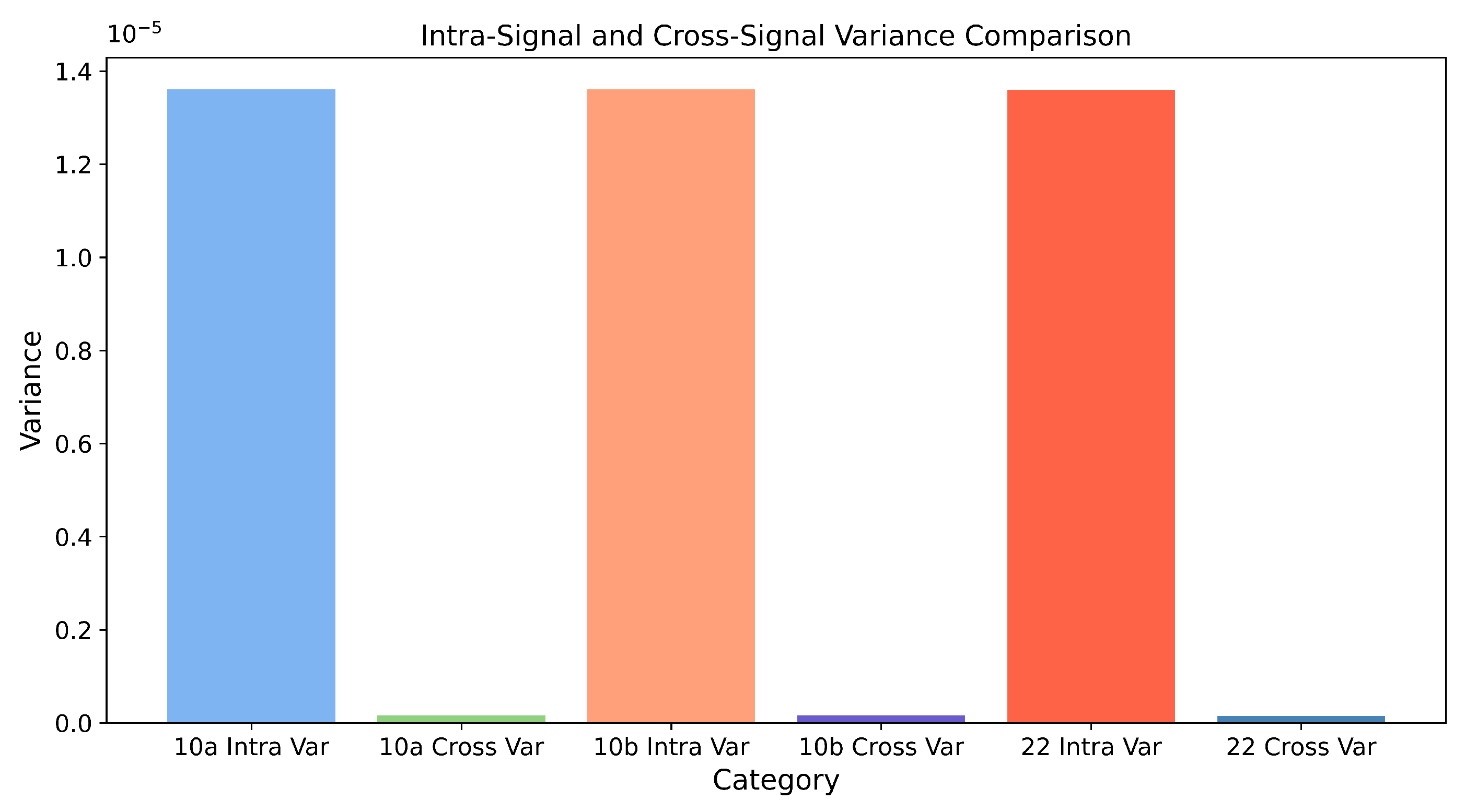
For AMR tasks, as in Figure 4, where the statistic is calculated from the CNN feature maps by feeding the RML2016.10a, RML2016.10b [31], and RML22 datasets [32]. The inputs demonstrate a regional statistic with large intra-signal variance and small cross-signal variance.The intra-signal variance is approximately 100 times that of the cross-signal variance. This suggests that for IQ signals, significant variations can occur at different time spans. How to enhance the adaptive capacity of the modulation recognition model at different moments of IQ signals will be the key to improving the recognition accuracy of the network.

3.3. Feature Enhancement Block (FE)

ViT demonstrates scalable architectures and excels in capturing global features. However, conventional vision transformer methods often use 3 × 3 convolutional projection during the feature embedding phase for signal classification. Adapting this approach to signal classification may overlook key signal characteristics, as detailed in VT-MCNet. To improve the feature extraction process in transformer networks, especially for tasks requiring the ability to adapt to IQ signals that varies continuously with time characteristics, we intend to utilize the TVConv (Translation Variant Convolution) for the feature extraction component. This helps the model better adapt to the characteristic of IQ signal changing over time. The TVConv methodology introduces two primary units: the Affinity Map Unit (AMU) and the Weight-Generating Unit (WGU), which collectively enhance the network’s ability to adapt to spatial variances within the signal.

3.3.1. Affinity Map Unit (AMU)

The Affinity Map Unit (AMU) is a crucial component of TVConv, designed to capture the correlation between IQ signals at adjacent time instants. This unit generates learnable affinity maps, which help in understanding the contextual importance of different segments of the IQ signal. The process involves several key steps:
  • Learnable Affinity Maps: These maps are trained to highlight the connections between various samples in the IQ signal. Similar to attention mechanisms used in transformers, these affinity maps reduce the computational overhead while capturing essential spatial relationships.
  • Spatial Awareness: By focusing on relationships between pairs of time steps within the IQ sequence, the AMU can distinguish between different characteristics of the IQ signal, such as phase shifts, frequency changes, and amplitude variations, ensuring a nuanced understanding of the signal’s structure.
  • Implementation Details: The AMU employs a learnable function f to compute the affinity between each pair of time steps ( i , j ) within the IQ signal. This function takes into account the temporal position and signal characteristics, such as amplitude and phase, producing a matrix of affinities. A.
Mathematically, the affinity maps A are generated as follows:
A i , j = f ( x i , x j ; θ )
where x i and x j are the feature vectors of the IQ sequence at time steps i and j, respectively, and θ represents the parameters of the learnable function f. The function f can be modeled using a neural network that takes the concatenated feature vectors of these time-step pairs and outputs a scalar affinity score.
The affinity map A then undergoes a normalization process, often using a softmax function to ensure that the affinities for each time step sum to one, providing a probabilistic interpretation.

3.3.2. Weight-Generating Unit (WGU)

The Weight-Generating Unit (WGU) leverages the affinity maps produced by the AMU to generate sample-specific convolutional weights. This unit ensures that the convolution operation adapts dynamically to different segments of the IQ signal, enhancing feature extraction and improving overall performance. The WGU consists of several steps:
  • Weight Generation: The WGU produces convolutional weights tailored to each spatial location, using the affinity maps to ensure these weights are contextually relevant. The process involves a learnable function g that maps the affinities to convolutional weights.
  • Efficiency: To maintain computational efficiency, the weights can be precomputed and stored, allowing for fast retrieval during the inference phase.
  • Implementation Details: The function g used in the WGU is designed to take the affinity maps and generate the appropriate weights for each convolutional filter. This function can be implemented using a neural network that outputs a set of weights for each time step based on the affinity values.
The weights W for the convolution operation are computed as:
W i , j = g ( A i , j ; ϕ )
where ϕ represents the parameters of the learnable function g. The function g transforms the normalized affinities into convolutional weights, ensuring that each pixel’s convolutional operation is influenced by its spatial context.

3.4. Transformer Encoder with SKAT Framework

3.4.1. Multi-Head Self-Attention

Multi-Head Self-Attention (MHSA) is a crucial component of the transformer architecture, representing each token as a weighted sum of all other tokens to capture intricate dependencies and relationships within the input sequence. For each element in the sequence:
Q = X W Q , K = X W K , V = X W V
The attention scores are computed as:
Attention ( Q , K , V ) = softmax Q K T d k V
To capture different aspects of the sequence:
MHSA ( X ) = Concat head 1 , head 2 , , head N h W O

3.4.2. SKAT Framework

The Skip-Attention enhances computational efficiency by reducing redundant computations in the self-attention mechanism. It leverages the high correlation in self-attention maps across different layers. Instead of computing self-attention in every layer, SKAT reuses representations from previous layers through a parametric function.
The SKAT parametric function Φ approximates the output of skipped self-attention layers:
Z l M S A Φ ( Z l 1 M S A )
Z l M S A = ECA ( FC 2 ( DwC ( FC 1 ( Z l 1 M S A ) ) ) )
where FC 1 and FC 2 are fully connected layers, DwC [33] represents depth-wise convolution, and ECA [34] denotes efficient channel attention.

3.4.3. Transformer Encoder with SKAT

The SKAT-modified transformer layer updates the representation as follows:
Z l Φ ( Z l 1 M S A ) + Z l 1
Z l MLP ( Z l ) + Z l
where MLP denotes the multi-layer perceptron applied to the output.
The Transformer Encoder, enhanced by the SKAT framework, provides a robust and efficient method for processing sequential data. By leveraging the high correlation in self-attention maps, SKAT reduces redundant computations, thereby improving throughput and reducing FLOPs without compromising performance.

4. Experimental Results and Discussion

4.1. Datasets

To evaluate the performance of the proposed method, we conduct experiments on the RadioML2016.10a [31], RadioML2016.10b, and RML22 [32] datasets. The datasets comprise eight digital modulated signals widely used in wireless communications, including 8PSK, BPSK, CPFSK, GFSK, PAM4, 16QAM, 64QAM, and QPSK. Each sample includes in-phase and quadrature (IQ) channels. The SNR ranges from 20 dB to 18 dB with an interval of 2 dB. Signals are modulated at a rate of eight samples per symbol. In addition, random walk drifting of the carrier frequency oscillator, additive white Gaussian noise (AWGN), and Rician fading of the channel impulse response are taken into account in the process of generating signals. Furthermore, translation, dilation, and unknown scale are introduced when the signal is transmitted through harsh channels. In conclusion, all 11 modulation types are employed to form both the training and testing datasets, thereby ensuring a thorough evaluation of the models across the entire range of modulation types. The details of the experimental dataset are shown in Table 1.
All experiments are conducted on the Nvidia GeForce RTX 2080Ti 11G GPU. In the training process, the deep learning framework is Pytorch. The training parameters are shown in Table 2. In the testing stage, to avoid the contingency caused by a single test, we use the average accuracy of 100 test experiments as the final evaluation indicator. The calculation formula a c c of a single test is defined as:
a c c = ( N t r u e N a l l ) × 100 %
where N t r u e is the number of samples correctly classified and N a l l is the number of all samples.

4.2. Analysis of Feature Enhance Module

4.2.1. Performance Comparisons with Different Parameters in the Weight-Generating Block

To evaluate the classification performance of the FEVCT under different parameters, we examine the role of different components, including the depth (layers), width (channels) of the weight-generating block B, and the number of channels in affinity maps A.
Ablation under the varied number of channels and inter layers for weight generating block B, as well as the varied number of channels for affinity maps A. We use hyper-parameters highlighted in bold as our default setting elsewhere in the paper.
According to Table 3 and Table 4, we examine the role of different components, including the width (channels) of the weight-generating block B and the number of channels in affinity maps A. With deeper, wider layers in B or more channels in A, the model generally performs better. However, the performance slightly drops from the peak when the overparameterization goes too far. This is because a larger model might require more iterations for training and can suffer from overfitting.
From Table 5, the classification accuracy of FE-SKViT when the number of layers in the weight-generating block, B, is 5( B L a y e r s = 5 ). significantly outperforms that at B L a y e r s = 1 , 2 , 3 , 4 and B L a y e r s = 6 . When B L a y e r s = 5 , the FE-SKViT stands out with the highest overall accuracy of 63.326% and the lowest minimum verification loss of 1.03231. This configuration achieves optimal performance, balancing model complexity and efficiency. However, increasing the layer count to 6 or decreasing it to 4, 3, 2, or 1 results in the rate of improvement in classification accuracy slowing down, indicating that 5 layers provide the best trade-off between accuracy and computational efficiency. In the following part, we set B L a y e r s = 5 to construct the FE-SKViT.

4.2.2. Recognition Performance by SNR and Modulation Type

We fix the hyper-parameters BLayers, Bchans and AChans of FE-SKViT as 5, 64, and 4 and evaluate its performance by SNR and modulation type.
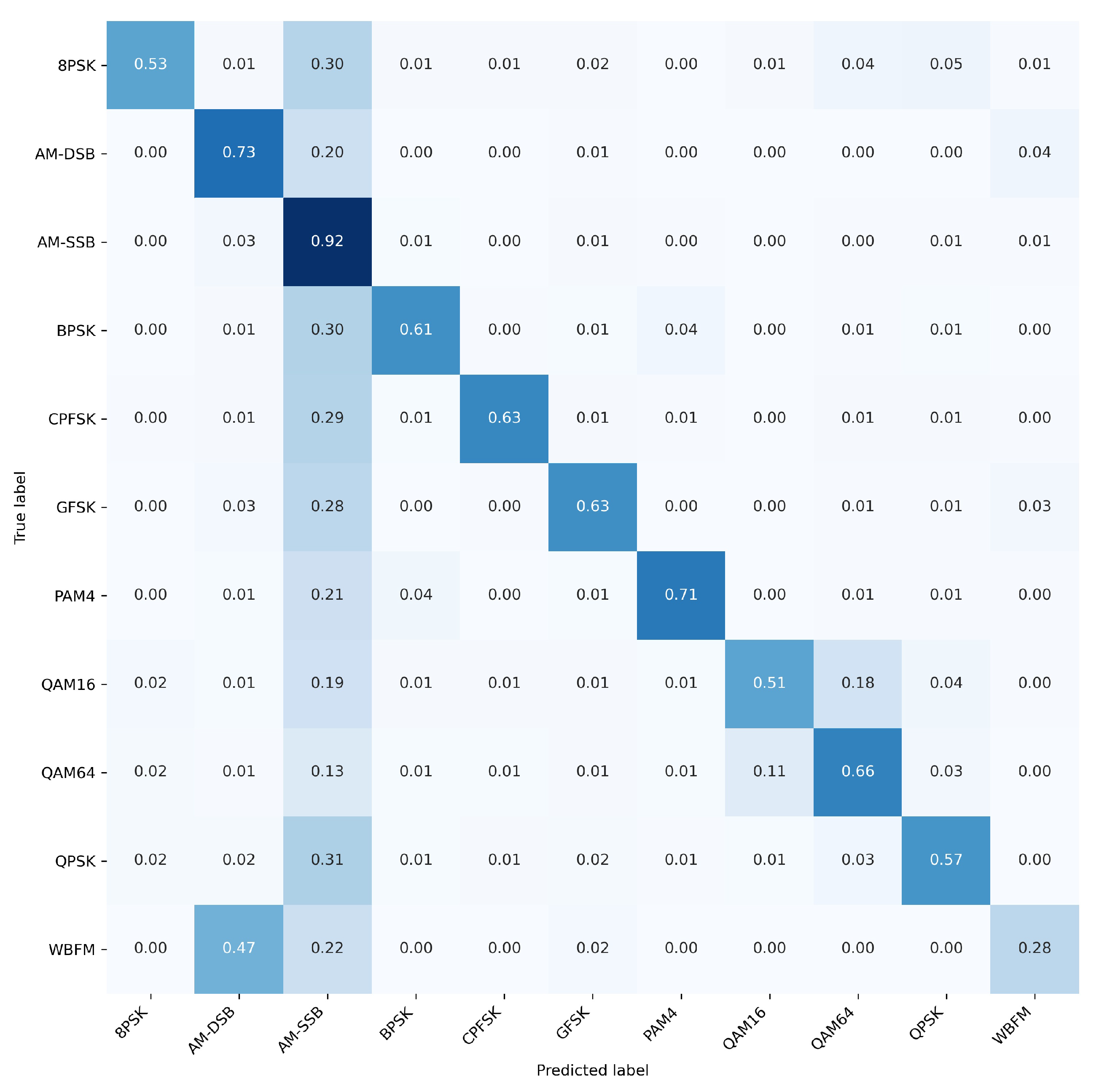
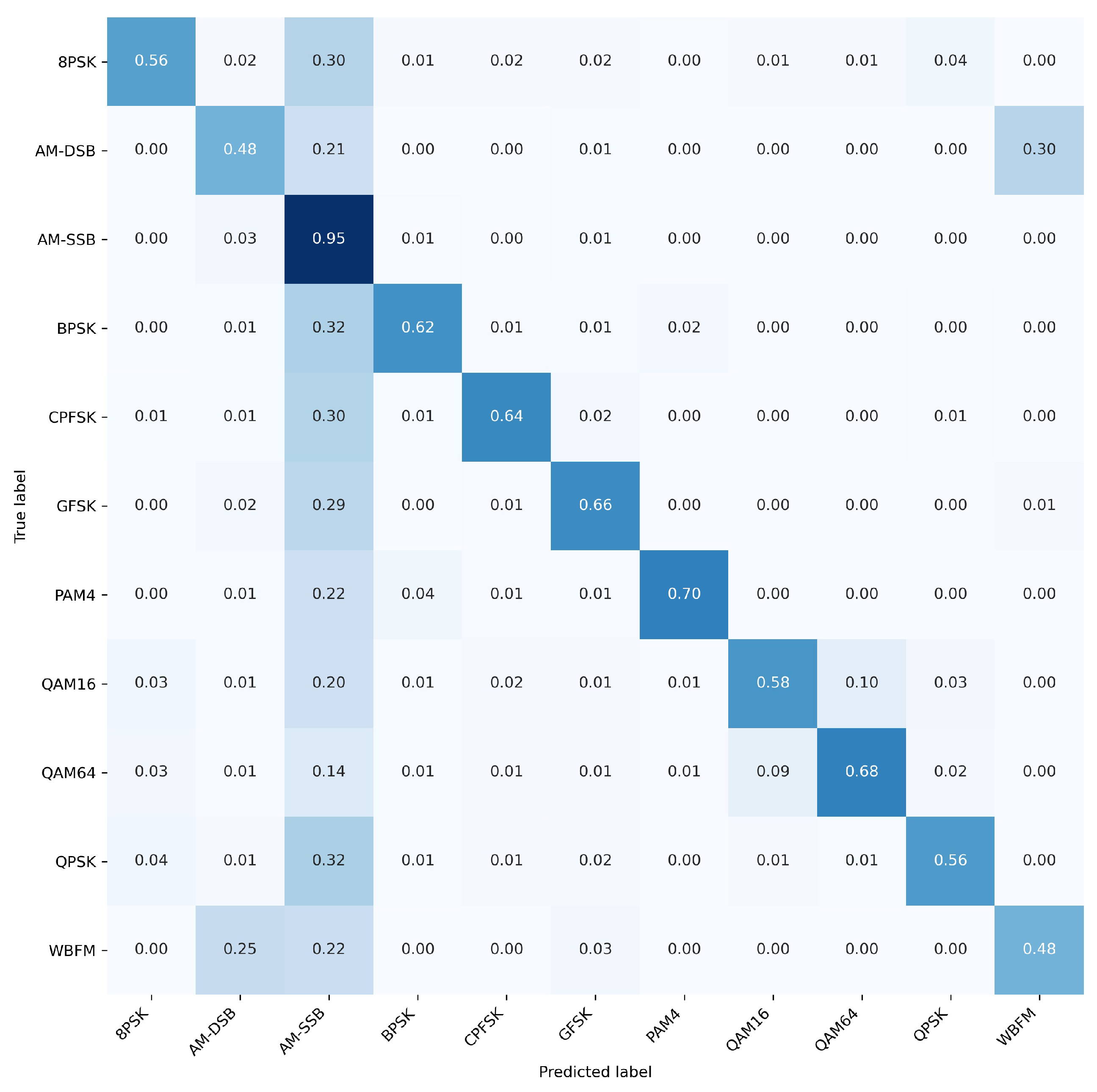
Based on the comparison of the confusion matrices of the two models, as illustrated in Figure 5 and Figure 6, it was found that incorporating the translation variant block improved the model’s recognition rates for modulation schemes including QAM16, QAM64, WBFM, BPSK, and AM-SSB. But the recognition rate of the AM-DSB modulation mode has declined severely. Table 6 provides a detailed comparison of the experiments conducted at −2 dB.
The data presented in Table 6 indicate that the FE-ViT model consistently outperforms the ViT model across most scenarios, achieving an overall recognition accuracy of 83.98%, compared to 80.56% for the ViT model. Notably, the FE-ViT model demonstrates significantly enhanced performance on QAM16 and QAM64 modulation schemes, with accuracies of 84.50% and 90.19%, respectively, in contrast to the ViT model’s performances of 74.00% and 80.88%. Furthermore, a substantial improvement is observed in WBFM for the FE-ViT model, which attains an accuracy of 54.50%, as opposed to just 31.00% for its counterpart. Both models exhibit equivalent performance on BPSK, each achieving an accuracy of 94.94%. However, it is important to note that the ViT model slightly surpasses the FE-ViT model in AM-DSB modulation with an accuracy of 88.01%, compared to the latter’s score of 64.89%. Due to the error occurring in the generation of the analog information source in [32] within RML2016.10a, the low recognition rate of AM-DSB holds scant reference value, as described.
In summary, while both models have their merits, the FE-ViT exhibits superior capabilities particularly concerning higher-order modulation schemes and frequency modulation.
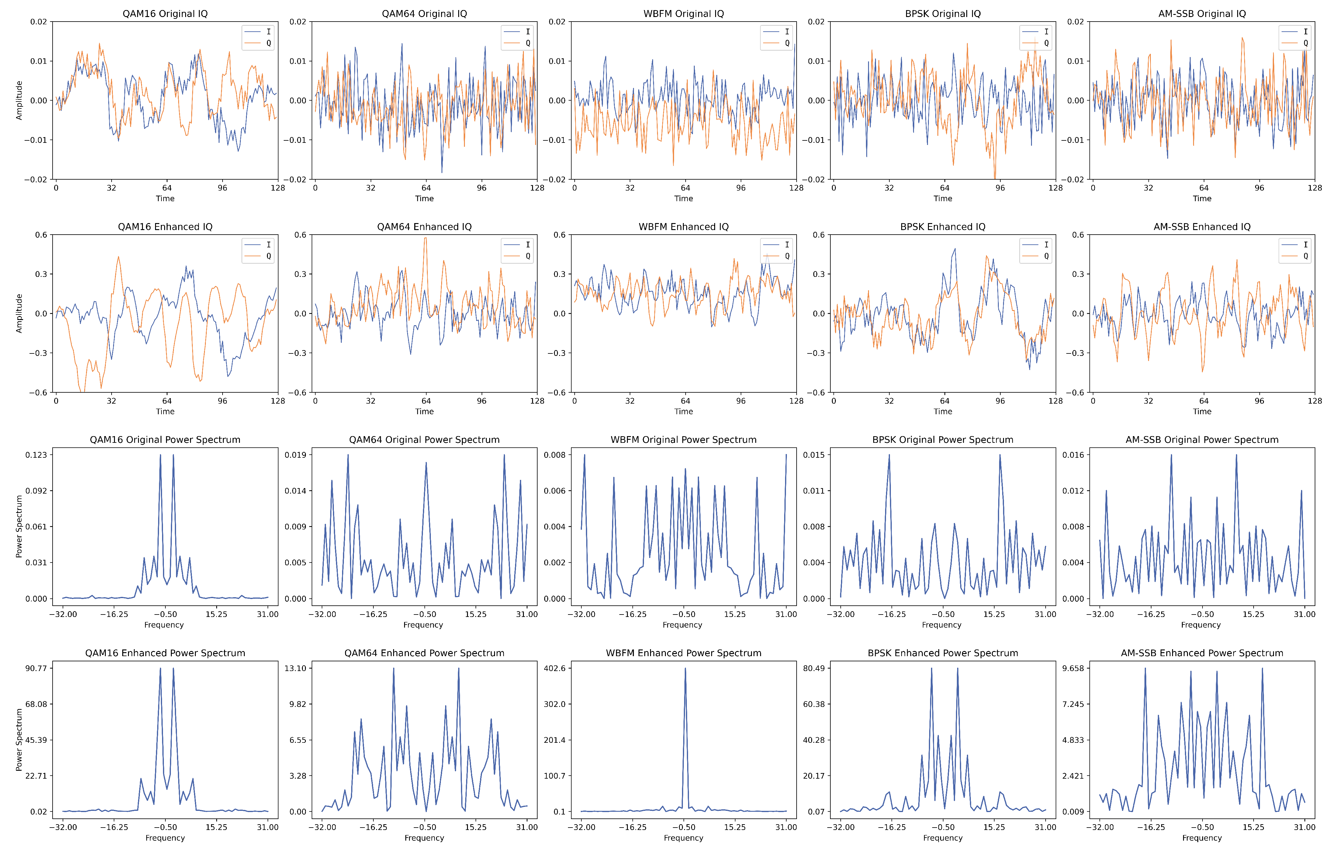
Figure 7 illustrates the effects of a feature-enhanced module for these five modulation schemes.

4.2.3. Feature Visualization

As shown in Figure 7, the initial IQ diagram of QAM16 displays significant noise and irregularity. Following enhancement, it reveals a smoother and more distinguishable signal pattern. The power spectrum also exhibits improved frequency resolution and clearer peaks. Quantitatively, the noise amplitude of the original IQ signal ranges from −0.02 to 0.02, whereas the enhanced signal is notably reduced to between −0.3 and 0.6, thereby improving signal clarity substantially. The original power spectrum presents broad and noisy peaks; however, after enhancement, sharper peaks at critical frequencies are attained, with background noise diminished by approximately 60%.
In the original IQ diagram of QAM64, substantial noise and fluctuations hinder effective signal discrimination. Post-enhancement, both the noise level decreases and clarity improves; nevertheless, the inherent complexity of QAM64 persists as a challenge. The peak in the power spectrum is better defined with reduced noise levels observed overall. Numerically speaking, the fluctuations in the IQ diagram decrease from an initial range of −0.02 to +0.02 to a post-enhancement range of −0.3 to +0.6; concurrently, mid-frequency band signals exhibit more pronounced peaks while background noise diminishes by about 55%.
The initial IQ plot for WBFM contains considerable noise and irregularities; however, in its enhanced version, there is significant suppression of this noise, leading to clearer signal patterns emerging thereafter. The initially broad and noisy power spectrum becomes increasingly concentrated following enhancement efforts undertaken herewith: quantitatively assessed fluctuations within the original IQ signal span from −0.02 to +0.02 but are suppressed downwards into a range between −0.3 and +0.6 upon enhancement application—resulting in nearly a 70% reduction in background noise that now concentrates around central frequencies.
The initial BPSK IQ map demonstrates elevated levels of both noise as well as irregular fluctuations; yet, subsequent enhancements yield decreased levels thereof alongside increased stability within resultant signals produced hereinafter—a transformation wherein previously broad spectra characterized by multiple noisy peaks evolve into distinctly clear singular peak states instead. We specifically note that prior ranges for such noises transition from an interval spanning −0.02 through +2.00 towards one confined strictly between values ranging thusly −0.3 through +0.6, accompanied by notable improvements across respective spectral domains, reflecting reductions approximating 65%.
Lastly, addressing AM-DSB’s original I/Q plots which reveal extensive amounts pertaining toward both noisiness along with erratic patterns present therein, enhanced versions demonstrate marked interference reductions, yielding coherent characteristics conducive towards identification purposes henceforth achieved via concentration focused sharply upon single prominent peak formations rather than diffuse distributions seen earlier on display whereupon noted fluctuation intervals originally ranged broadly −0.02 up until +0.02. These are subsequently compressed downwards, ultimately residing firmly nestled amid tighter confines, extending only throughout limits established above, i.e., −0.3 through +0.6, finally culminating in overall reductions nearing 75% with respect to residual ambient disturbances.
In a word, the feature enhancement module significantly enhances signal quality across various modulation schemes. Enhanced IQ plots consistently show reduced noise and clearer signal patterns. Enhanced power spectrum exhibit more defined peaks and reduced noise, indicating improved frequency resolution. This demonstrates the feature enhancement module’s effectiveness in enhancing signal recognition by improving the clarity and stability of IQ diagrams and power spectra across all tested modulation schemes.

4.3. Ablation Study

As shown in Table 7, FE-SKViT stands out with the highest performance among the models. FE-SKViT’s average accuracies are 63.31 on RML16a, 65.05 on RML16b, and 68.3 on RML22, making it the most accurate, especially on the RML22 dataset. Its superior accuracy highlight its advantage over other models. Subsequently, we standardized the model parameter configurations to enable a consistent comparison of model complexities across different architectures, as shown in Table 8 and Table 9.
The integration of the SKIP module in FE-SKViT results in a notable increase in memory consumption compared to FE-ViT, escalating from 11.76 MB to 35.44 MB. This increase can be attributed to the additional intermediate computations and storage demands imposed by the SKIPAT module. Despite this increase in memory usage, there is a slight enhancement in inference speed, improving from 0.0114 s to 0.0130 s. This improvement stems from SKIPAT’s ability to bypass redundant computations, particularly by reusing attention maps and reducing the number of times the expensive self-attention mechanism needs to be recalculated. As a result, the model achieves a faster forward pass, demonstrating that the trade-off between increased memory consumption and reduced computation can lead to overall performance gains in terms of inference time.

4.4. Performance Comparisons to the State-of-the-Art

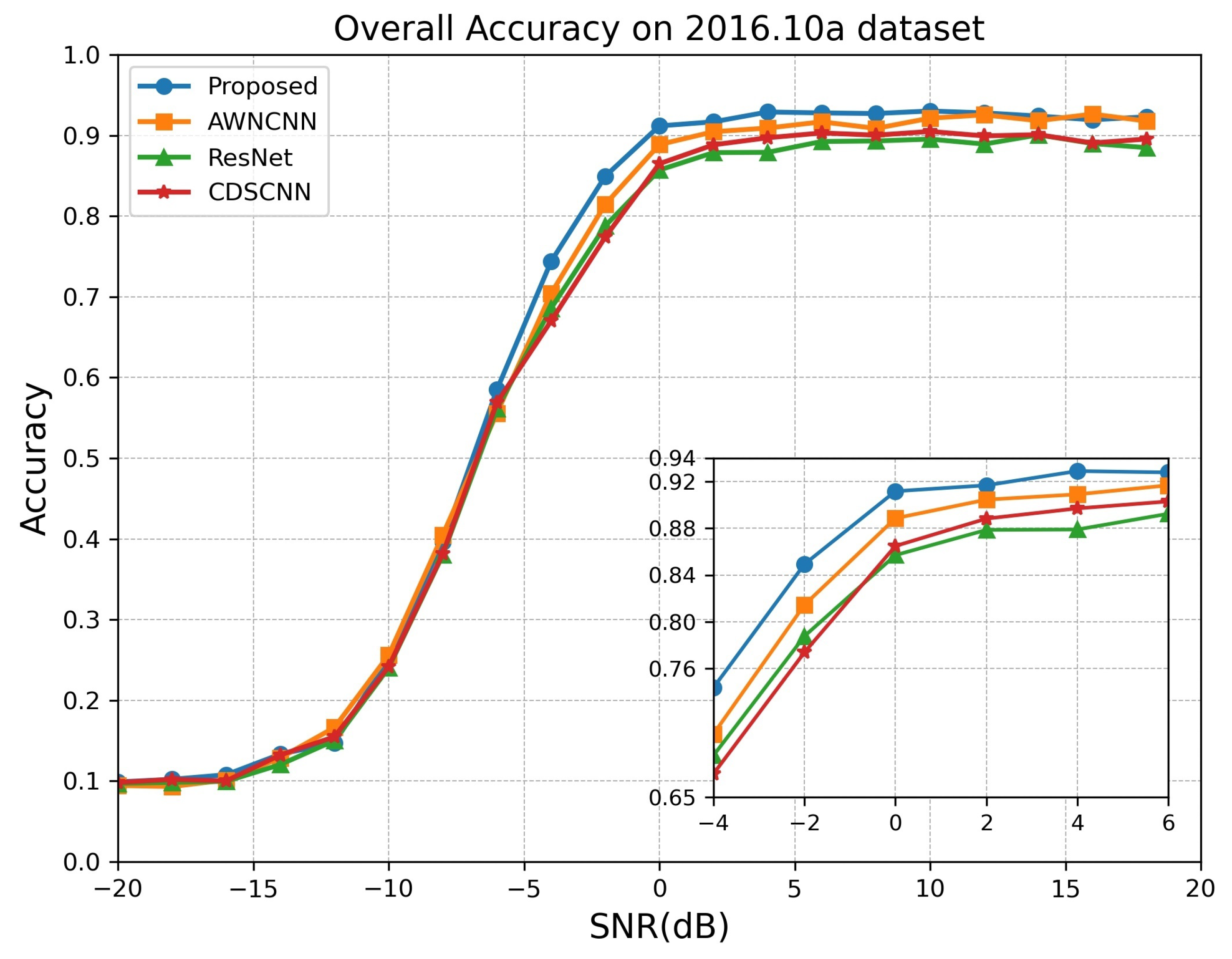
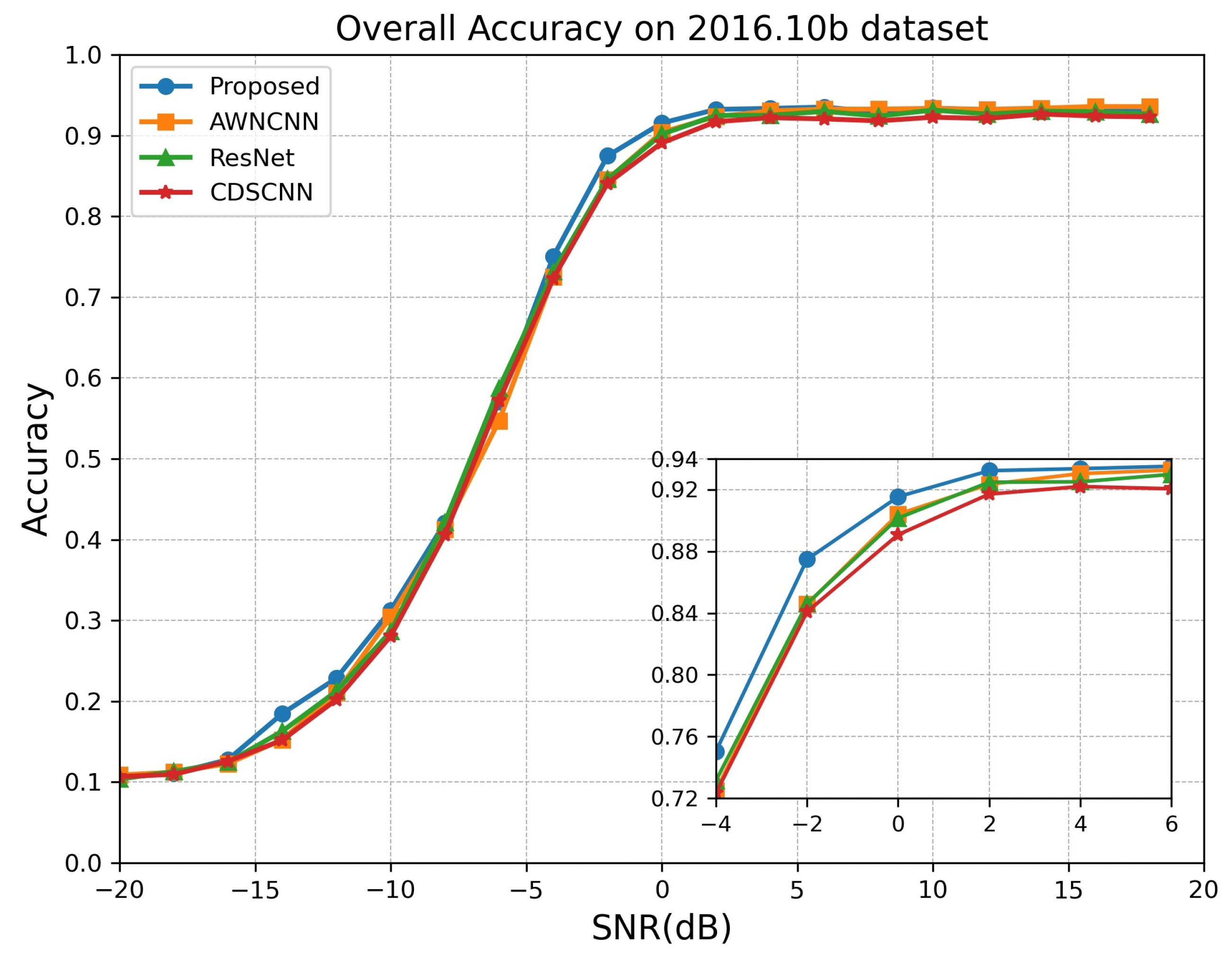
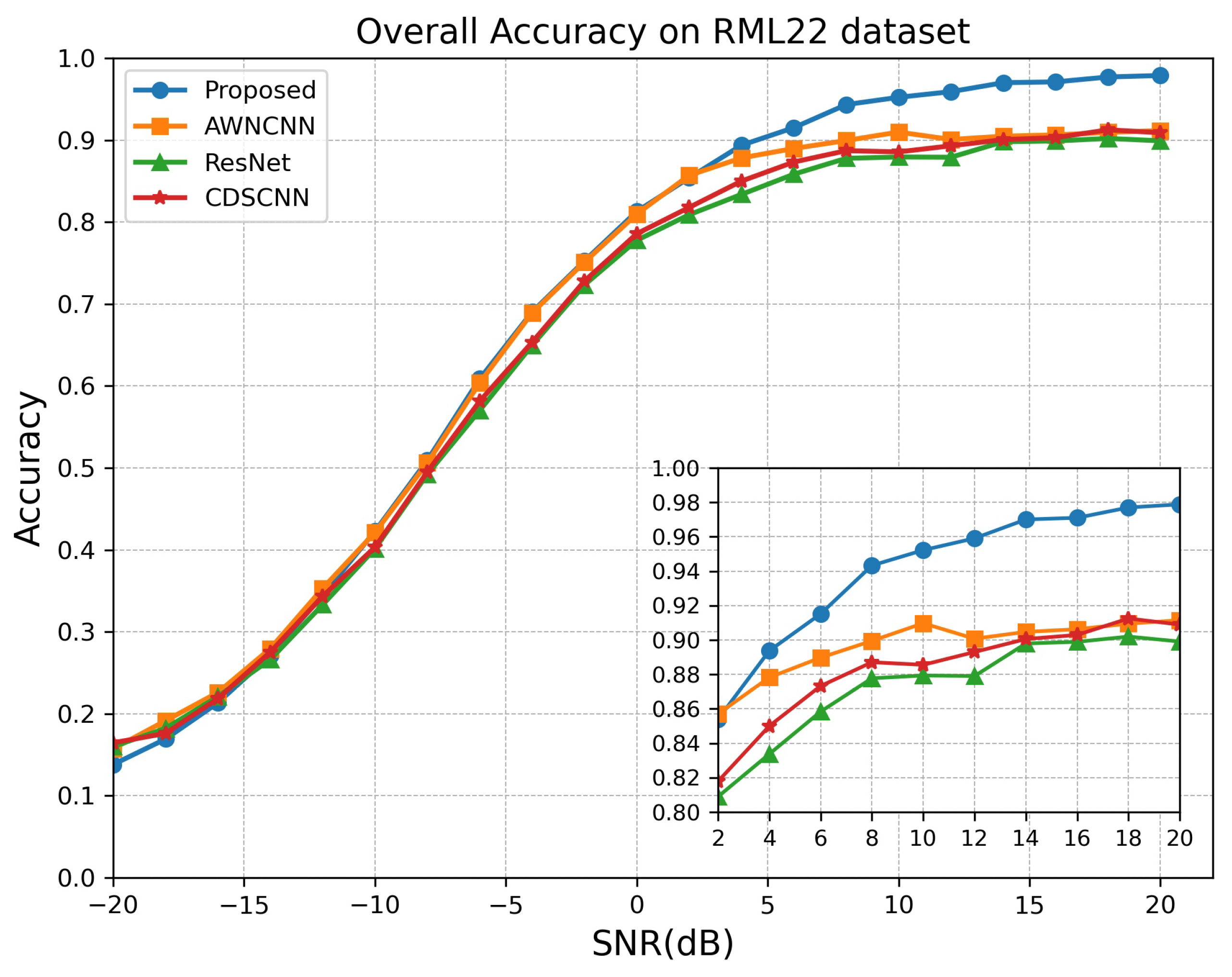
To evaluate the performance of the FE-SKViT presented in this paper, we compared it against four different methods: the adaptive wavelet network (AWN) [35], the deep residual network (ResNet18) [36], the complex-valued depth-wise separable convolutional neural network (CDSCNN) [37], and the Feature-Enhanced Transformer with skip attention (FE-SKViT). The experimental results under different feature extraction modules are illustrated in Figure 8, Figure 9 and Figure 10. Table 10 summarizes the various methods proposed in this paper.
As shown in Table 10, The ResNet18 model includes multiple ResBlocks, each containing a 2D convolution (Conv2d) with a kernel size of 3 × 3, BatchNorm (BN) for normalization to speed up convergence, ReLU as the activation function, and a MaxPooling layer (MaxPool2D) with a kernel size of 2 × 2 to reduce data dimensions. The ResNet18 architecture is composed of these ResBlocks followed by a Flatten layer for transforming the final feature maps into a one-dimensional array for classification.The CDSCNN architecture employs depth-wise separable convolutions to efficiently extract features. Each convolutional layer includes a depth-wise Conv2d followed by a point-wise Conv2d, both using a kernel size of 3 × 3. BatchNorm (BN) is applied after each convolution for normalization, and ReLU serves as the activation function. MaxPooling layers (MaxPool2D) with a kernel size of 2 × 2 are used for dimension reduction. The network ends with a Flatten layer to convert the data into a suitable format for the fully connected layers.The AWN integrates adaptive wavelet decomposition with channel attention mechanisms. Initially, the network comprises Conv2d layers with a kernel size of 3 × 3, followed by BatchNorm (BN) for normalization and ReLU activation functions. MaxPooling layers (MaxPool2D) with a kernel size of 2 × 2 are used to downsample the data. The adaptive wavelet decomposition further refines feature extraction across multiple frequency bands. An attention mechanism is applied to emphasize significant features, and a Flatten layer is used to prepare the data for the final classification stages. The FE-SKViT is illustrated in Figure 1.
We fix the hyper-parameters BLayers, Bchans, and AChans of FE-SKViT as 5, 64, and 4, for a good balance of accuracy and Complexity according to Table 7, and evaluate its performance by SNR and modulation type.The recognition accuracy comparison of FE-SKViT and baseline methods is shown in Table 11.
According to Figure 8, it can be seen that on RML2016.10a, when the SNR is less than −8 dB, FE-SKViT performs slightly weaker than some baseline methods, while when the SNR is greater than −8 dB, FE-SKViT performs better, especially at the −6 to 6 dB SNR range. However, for SNR values above 6 dB, FE-SKViT’s performance is comparable to that of the baseline methods. On the whole, FE-SKViT outperforms the baseline methods by 2.92%, 2.49%, and 1.05% with respect to average accuracy.
According to Figure 9, it can be seen that on RML2016.10b, the FE-SKViT obtains better recognition accuracy than the baseline methods over almost the entire −16 to 6 dB SNR range, and that advantage is more evident at −4 to 6 dB SNRs. On the whole, FE-SKViT outperforms the baseline methods by 0.86%, 1.53%, and 0.87% on the average accuracy.
According to Figure 10, it can be seen that on RML22, when the SNR is less than −10 dB, FE-SKViT performs slightly weaker than some baseline methods, while when the SNR is greater than −10 dB, FE-SKViT performs always better, especially for the 2 to 20 dB SNR range. On the whole, FE-SKViT outperforms the baseline methods by 0.86%, 1.53%, and 0.87% on the average accuracy.
In a word, the FE-SKViT achieves the SOTA recognition performance on RML2016.10a, RML2018.01a, and RML22.

5. Conclusions

In this paper, to solve the problem of automatic modulation recognition of communication signals under conditions of low SNR, a novel model FE-SKViT that can extract local features of signals is proposed. The FE component is utilized to handle large intra-signal variance and small cross-signal variance by employing learnable affinity maps and a weight-generating block, while the SKAT component effectively improving accuracy by skipping redundant self-attention computations across layers. We validated the performance of FE-SKViT on three benchmark datasets, i.e., RML2016.10a, RML2016.10b, and RML22, with recognition accuracy higher than some current mainstream AMR models and robustness to noise. Furthermore, we designed a series of ablation studies and a visualization analysis to demonstrate the effectiveness of the FE-SKViT model. Moreover, the proposed model integrates the SKAT component, resulting in higher recognition accuracy with higher computational and storage cost. The model’s recognition accuracy does not exhibit significant improvement under high SNR conditions. Future works will focus on feature extraction, such as Multi-Frequency Octave [38], Masked Signal Feature Extractor [39], and other content [40,41], to improve performance in actual scenarios. In addition, reducing the complexity of the proposed model is also a direction worth exploring.

Author Contributions

Conceptualization, G.Z. and B.Z.; methodology, G.Z., B.Z. and P.Y.; software, G.Z. and W.Z.; validation, G.Z., B.Z., W.Z. and B.L.; formal analysis, W.Z. and B.L.; investigation, G.Z., B.Z. and P.Y.; resources, B.Z., W.Z. and B.L.; data curation, B.L.; writing—original draft preparation, G.Z. and B.Z.; writing—review and editing, G.Z. and B.Z.; supervision, B.Z., P.Y. and W.Z.; project administration, B.Z. and P.Y.; funding acquisition, B.Z. and P.Y. All authors have read and agreed to the published version of the manuscript.

Funding

This research received no external funding.

Data Availability Statement

In this paper, the RadioML2016.10a, RadioML2016.10b, and RadioML22 datasets are employed for experimental verification. The RadioML2016.10a dataset is a representative dataset for the testing and evaluation of current AMR methods. Readers can obtain the dataset from the author by email ([email protected]).

Acknowledgments

I would like to acknowledge our colleagues for their wonderful collaboration and patient support. I also thank all the reviewers and editors for their great help and useful suggestions.

Conflicts of Interest

The authors declare no conflicts of interest.

References

  1. Wang, J.; Liu, X.; Zhang, Y.; Chen, H. Deep Learning Based Automatic Modulation Recognition: Models, Datasets, and Challenges. arXiv 2022, arXiv:2207.09647. [Google Scholar]
  2. Xia, H. Cellular signal identification using convolutional neural networks: AWGN and Rayleigh fading channels. In Proceedings of the 2019 IEEE International Symposium on Dynamic Spectrum Access Networks (DySPAN), Newark, NJ, USA, 11–14 November 2019. [Google Scholar]
  3. Peng, S.; Sun, S.; Yao, Y.D. A survey of modulation classification using deep learning: Signal representation and data preprocessing. IEEE Trans. Neural Netw. Learn. Syst. 2021, 33, 7020–7038. [Google Scholar] [CrossRef] [PubMed]
  4. Jiang, X.R.; Chen, H.; Zhao, Y.D.; Wang, W.Q. Automatic modulation recognition based on mixed-type features. Int. J. Electron. 2021, 108, 105–114. [Google Scholar] [CrossRef]
  5. Zhang, D.; Lu, Y.; Li, Y.; Ding, W.; Zhang, B.; Xiao, J. Frequency Learning Attention Networks based on Deep Learning for Automatic Modulation Classification in Wireless Communication. Pattern Recognit. 2023, 137, 109345. [Google Scholar] [CrossRef]
  6. Xu, J.L.; Su, W.; Zhou, M. Likelihood-ratio approaches to automatic modulation classification. IEEE Trans. Syst., Man, Cybern. C Appl. Rev. 2011, 41, 455–469. [Google Scholar] [CrossRef]
  7. Al-Sa’d, M.; Boashash, B.; Gabbouj, M. Design of an optimal piece-wise spline wigner-ville distribution for TFD performance 365 evaluation and comparison. IEEE Trans. Signal Process 2021, 69, 3963–3976. [Google Scholar] [CrossRef]
  8. Abd-Elaziz, O.F.; Abdalla, M.; Elsayed, R.A. Deep learning-based automatic modulation classification using robust CNN architecture for cognitive radio networks. Sensors 2023, 23, 9467. [Google Scholar] [CrossRef]
  9. Wang, X.; Li, Y.; Zhang, P.; Wang, Z. RNN-based melody generation using sequence-to-sequence learning. IEEE Access 2019, 7, 165346–165356. [Google Scholar]
  10. Sainath, T.N.; Vinyals, O.; Senior, A.; Sak, H. Convolutional, long short-term memory, fully connected deep neural networks. In Proceedings of the 2015 IEEE International Conference on Acoustics, Speech and Signal Processing (ICASSP), South Brisbane, QLD, Australia, 19–24 April 2015; pp. 4580–4584. [Google Scholar]
  11. Tu, Y.; Lin, Y. Deep neural network compression technique towards efficient digital signal modulation recognition in edge device. IEEE Access 2019, 7, 58113–58119. [Google Scholar] [CrossRef]
  12. Lee, S.H.; Kim, K.-Y.; Kim, J.H.; Shin, Y. Effective feature-based automatic modulation classification method using DNN algorithm. In Proceedings of the 2019 International Conference on Artificial Intelligence in Information and Communication (ICAIIC), Okinawa, Japan, 11–13 February 2019; pp. 557–559. [Google Scholar]
  13. Shi, J.; Hong, S.; Cai, C.; Wang, Y.; Huang, H.; Gui, G. Deep learning based automatic modulation recognition method in the presence of phase offset. IEEE Access 2020, 8, 42841–42847. [Google Scholar] [CrossRef]
  14. Hiremath, S.M.; Behura, S.; Kedia, S.; Deshmukh, S.; Patra, S.K. Deep learning-based modulation classification using time and stockwell domain channeling. In Proceedings of the 2019 National Conference on Communications (NCC), Bangalore, India, 20–23 February 2019; pp. 1–6. [Google Scholar]
  15. Peng, S.; Jiang, H.; Wang, H.; Alwageed, H.; Zhou, Y.; Sebdani, M.M.; Yao, Y.D. Modulation classification based on signal constellation diagrams and deep learning. IEEE Trans. Neural Netw. Learn. Syst. 2019, 30, 718–727. [Google Scholar] [CrossRef] [PubMed]
  16. Wang, D.; Zhang, M.; Li, Z.; Li, J.; Fu, M.; Cui, Y.; Chen, X. Modulation format recognition and OSNR estimation using CNN-based deep learning. IEEE Photon. Technol. Lett. 2017, 29, 1667–1670. [Google Scholar] [CrossRef]
  17. Li, Y.; Shao, G.; Wang, B. Automatic modulation classification based on bispectrum and CNN. In Proceedings of the 2019 IEEE 8th Joint International Information Technology and Artificial Intelligence Conference (ITAIC), Chongqing, China, 24–26 May 2019; pp. 311–316. [Google Scholar]
  18. Mendis, G.J.; Wei, J.; Madanayake, A. Deep learning-based automated modulation classification for cognitive radio. In Proceedings of the 2016 IEEE International Conference on Communication Systems (ICCS), Shenzhen, China, 14–16 December 2016; pp. 1–6. [Google Scholar]
  19. Huang, S.; Jiang, Y.; Gao, Y.; Feng, Z.; Zhang, P. Automatic modulation classification using contrastive fully convolutional network. IEEE Wireless Commun. Lett. 2019, 8, 1044–1047. [Google Scholar] [CrossRef]
  20. Hu, S.; Pei, Y.; Liang, P.P.; Liang, Y.-C. Deep neural network for robust modulation classification under uncertain noise conditions. IEEE Trans. Veh. Technol. 2020, 69, 564–577. [Google Scholar] [CrossRef]
  21. Liu, Y.; Zhang, Y.; Wang, Z. A novel deep learning automatic modulation classifier with fusion of multichannel information using GRU. EURASIP J. Wirel. Commun. Netw. 2023, 2023, 66. [Google Scholar]
  22. Graves, A.; Fernández, S.; Schmidhuber, J. Bidirectional LSTM networks for improved phoneme classification and recognition. In Proceedings of the 15th International Conference on Artificial Neural Networks (ICANN), Warsaw, Poland, 11–15 September 2005; pp. 799–804. [Google Scholar]
  23. Chen, Y.; Li, Q.; Zhao, L.; Wang, M. Enhancing Automatic Modulation Recognition for IoT Applications Using Transformers. arXiv 2023, arXiv:2403.15417. [Google Scholar]
  24. Chen, Y.; Dong, B.; Liu, C.; Xiong, W.; Li, S. Abandon locality: Framewise embedding aided transformer for automatic modulation recognition. IEEE Commun. Lett. 2023, 27, 327–331. [Google Scholar] [CrossRef]
  25. Dosovitskiy, A.; Beyer, L.; Kolesnikov, A.; Weissenborn, D.; Zhai, X.; Unterthiner, T.; Dehghani, M.; Minderer, M.; Heigold, G.; Gelly, S.; et al. An Image is Worth 16x16 Words: Transformers for Image Recognition at Scale. arXiv 2020, arXiv:2010.11929. [Google Scholar]
  26. Dao, T.-T.; Noh, D.-I.; Pham, Q.-V.; Hasegawa, M.; Sekiya, H.; Hwang, W.-J. VT-MCNet: High-Accuracy Automatic Modulation Classification Model Based on Vision Transformer. IEEE Commun. Lett. 2024, 28, 98–102. [Google Scholar] [CrossRef]
  27. Worrall, D.E.; Garbin, S.J.; Turmukhambetov, D.; Brostow, G.J. Harmonic networks: Deep translation and rotation equivariance. In Proceedings of the IEEE Conference on Computer Vision and Pattern Recognition, Honolulu, HI, USA, 21–26 July 2017; pp. 5028–5037. [Google Scholar]
  28. Li, W.; Deng, W.; Wang, K.; You, L.; Huang, Z. A Complex-Valued Transformer for Automatic Modulation Recognition. IEEE Internet Things J. 2024, 11, 22197–22207. [Google Scholar] [CrossRef]
  29. Chen, J.; He, T.; Zhuo, W.; Ma, L.; Ha, S.; Chan, S.H.G. Tvconv: Efficient translation variant convolution for layout-aware visual processing. In Proceedings of the IEEE/CVF Conference on Computer Vision and Pattern Recognition, New Orleans, LA, USA, 18–24 June 2022; pp. 12548–12558. [Google Scholar]
  30. Venkataramanan, S.; Ghodrati, A.; Asano, Y.M.; Porikli, F.; Habibian, A. Skip-attention: Improving vision transformers by paying less attention. arXiv 2023, arXiv:2301.02240. [Google Scholar]
  31. O’shea, T.J.; West, N. Radio machine learning dataset generation with GNU radio. In Proceedings of the 6th GNU Radio Conference, Boulder, CO, USA, 12–16 September 2016; pp. 1–6. [Google Scholar]
  32. Sathyanarayanan, V.; Gerstoft, P.; Gamal, A.E. RML22: Realistic Dataset Generation for Wireless Modulation Classification. IEEE Trans. Wirel. Commun. 2023, 22, 7663–7675. [Google Scholar] [CrossRef]
  33. Chollet, F. Xception: Deep Learning with Depthwise Separable Convolutions. In Proceedings of the IEEE/CVF Conference on Computer Vision and Pattern Recognition (CVPR), Honolulu, HI, USA, 21–26 July 2017; pp. 1251–1258. [Google Scholar]
  34. Wang, Q.; Wu, B.; Zhu, P.; Li, P.; Zuo, W.; Hu, Q. ECA-Net: Efficient Channel Attention for Deep Convolutional Neural Networks. In Proceedings of the IEEE/CVF Conference on Computer Vision and Pattern Recognition (CVPR), Seattle, WA, USA, 13–19 June 2020; Volume 22, pp. 11534–11542. [Google Scholar]
  35. Zhang, J.; Wang, T.; Feng, Z.; Yang, S. Toward the Automatic Modulation Classification With Adaptive Wavelet Network. IEEE Trans. Cogn. Commun. Netw. 2023, 9, 549–563. [Google Scholar] [CrossRef]
  36. Liang, Z.; Tao, M.; Wang, L.; Su, J.; Yang, X. Automatic modulation recognition based on adaptive attention mechanism and ResNeXt WSL model. IEEE Commun. Lett. 2021, 25, 2953–2957. [Google Scholar] [CrossRef]
  37. Xiao, C.; Yang, S.; Feng, Z. Complex-valued Depth-wise Separable Convolutional Neural Network for Automatic Modulation Classification. IEEE Trans. Instrum. Meas. 2023, 72, 1–10. [Google Scholar]
  38. Hao, X.; Feng, Z.; Yang, S.; Wang, M.; Jiao, L. Automatic Modulation Classification via Meta-Learning. IEEE Internet Things J. 2023, 10, 12276–12292. [Google Scholar] [CrossRef]
  39. Wang, S.; Xing, H.; Wang, C.; Zhou, H.; Hou, B.; Jiao, L. SigDA: A Superimposed Domain Adaptation Framework for Automatic Modulation Classification. IEEE Trans. Wirel. Commun. 2024, 23, 13159–13172. [Google Scholar] [CrossRef]
  40. Chen, Y.; Shao, W.; Liu, J.; Yu, L.; Qian, Z. Automatic modulation classification scheme based on LSTM With random erasing and attention mechanism. IEEE Access 2020, 8, 154290–154300. [Google Scholar] [CrossRef]
  41. Huynh-The, T.; Pham, Q.-V.; Nguyen, T.-V.; Nguyen, T.T.; Costa, D.B.D.; Kim, D.-S. RanNet: Learning residual-attention structure in CNNsfor automatic modulation classification. IEEE Wirel. Commun. Lett. 2022, 11, 1243–1247. [Google Scholar] [CrossRef]
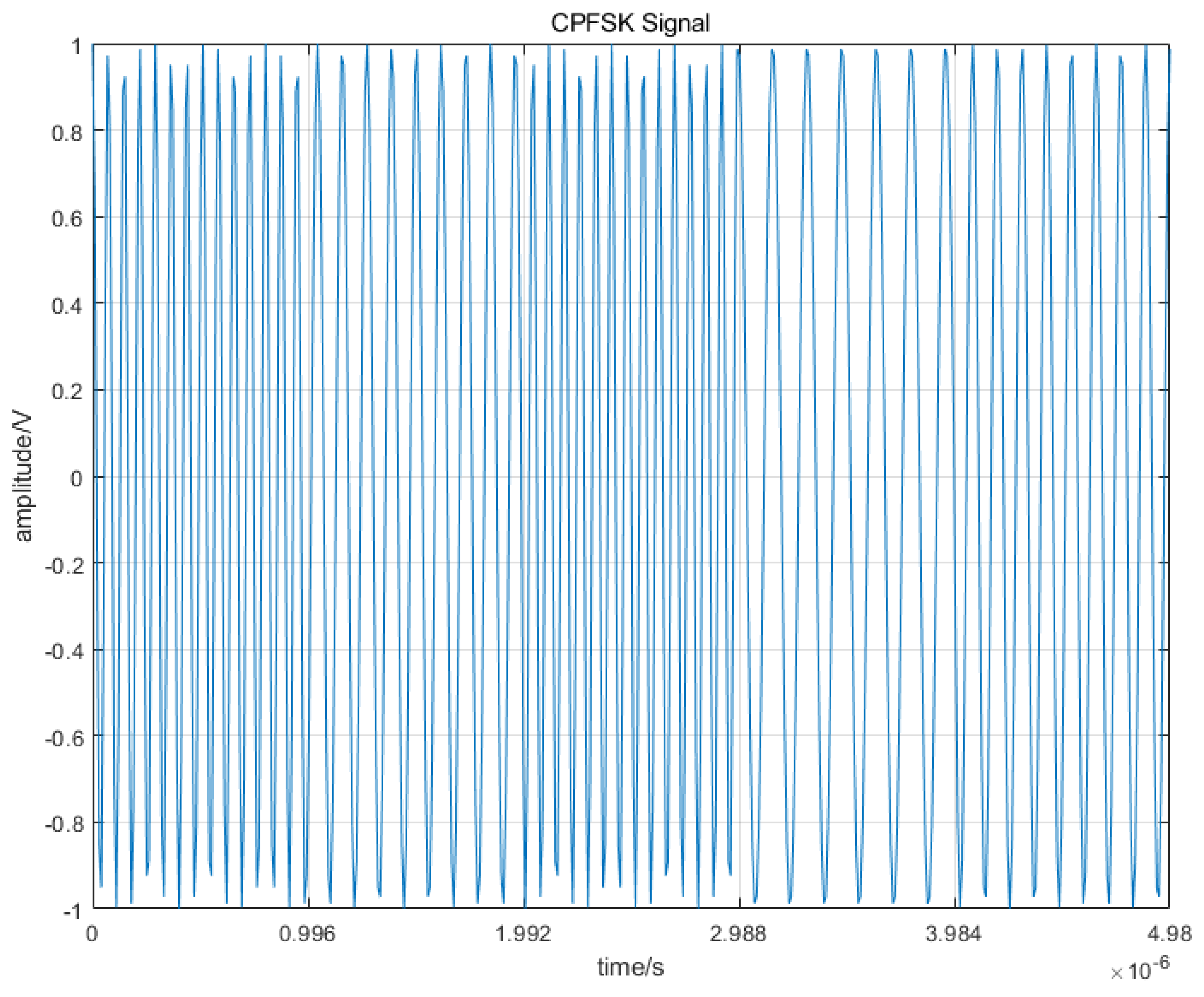
Figure 1. Waveform of the CPFSK signal, which is normalized.
Remotesensing 16 04204 g001
Figure 2. The architecture of FE-SKViT.
Remotesensing 16 04204 g002
Figure 3. The architecture of SKAT.
Remotesensing 16 04204 g003
Figure 4. Intra-signal and Cross-signal variance on RML datasets.
Remotesensing 16 04204 g004
Figure 5. Overall normalized confusion matrix of ViT on RML2016.10a.
Remotesensing 16 04204 g005
Figure 6. Overall normalized confusion matrix of FE-ViT on RML2016.10a.
Remotesensing 16 04204 g006
Figure 7. First channel of QAM16, QAM64, WBFM, BPSK, and AM-SSB signal samples (snr = −2 dB) after feature aggregation.
Remotesensing 16 04204 g007
Figure 8. Recognition accuracy comparison over different SNR levels on RML2016.10a.
Remotesensing 16 04204 g008
Figure 9. Recognition accuracy comparison over different SNR levels on RML2016.10b.
Remotesensing 16 04204 g009
Figure 10. Recognition accuracy comparison over different SNR levels on RML22.
Remotesensing 16 04204 g010
Table 1. The details of the experimental dataset.
ParameterRML2016.10aRML2016.10bRML22
ModulationsBPSK, QPSK, 8PSK, 16QAM, 64QAM, GFSK, CPFSK, PAM4, AM-DSB, AMSSB, WBFMBPSK, QPSK, 8PSK, 16QAM, 64QAM, PAM4, WBFM, CPFSK, GFSK, AM-DSBBPSK, QPSK, 8PSK, 16QAM, 64QAM, PAM4, WBFM, CPFSK, GFSK, AM-DSB
Signal dimension2 × 128(I/Q)2 × 128(I/Q)2 × 128(I/Q)
SNR range−20 dB:2 dB:18 dB−20 dB:2 dB:20 dB−20 dB:2 dB:20 dB
DistortionSample rate offset, Symbol rate offset, Selective fading, Center frequency offset, AWGN noiseThermal Noise, Sample rate offset, Center frequency offset, Channel effects, Doppler frequencyThermal Noise, Sample rate offset, Center frequency offset, Channel effects, Doppler frequency
Number of samples220,000420,000420,000
Split of training, validation, test8:1:18:1:18:1:1
Table 2. The training parameters.
ParametersValue
Learning rate0.0001
OptimizerAdamW
Loss FunctionCross-Entropy Loss
Episode300
Early stopping20
Table 3. Ablation under a varied number of channels for the weight-generating block.
BChansConvergence BatchMinimum Verification LossParameter (m)Overall Acc
1282361.037324.3762.926
722471.035421.7763.058
64401.032311.4863.326
322411.043460.5762.597
162361.049960.2462.357
82401.058100.1162.076
42481.079660.0560.673
Table 4. Ablation under a varied number of channels for the weight-generating block.
AChansConvergence BatchMinimum Verification LossTrainable ParamsOverall Acc
62381.04420389,56862.643
52441.03688388,99263.071
42401.03231388,41663.326
32361.03868387,84062.930
22481.03897387,26462.874
12431.03992386,68862.801
Table 5. Ablation under a varied number of layers for the weight-generating block.
BLayersConvergence BatchMinimum Verification LossParams Size (MB)Overall Acc
62381.037721.7563.048
52401.032311.4863.326
41941.036901.2263.031
32361.037280.9562.928
22421.040060.6862.693
12331.047080.4262.257
Table 6. Recognition accuracy at −2 dB SNR of each algorithm for five modulations.
ModelQAM16QAM64WBFMBPSKAM-DSBAM-SSBOverall Acc
ViT74.0080.8831.0094.9488.0193.1280.17
FE-ViT84.5090.1954.5094.9464.8995.7683.34
Table 7. The performances of ablation experiments on the three datasets.
DatasetModelOAMF1Kappa
RML2016.10aViT0.61840.64010.5801
FE-ViT0.62830.65830.5913
FE-SKViT0.63330.65970.5959
RML2016.10bViT0.64050.64120.5999
FE-ViT0.64450.64240.6044
FE-SKViT0.65030.64790.6106
RML2022ViT0.64830.63980.6087
FE-ViT0.66130.65410.6233
FE-SKViT0.68320.67880.6475
Table 8. The model parameters set for comparing the complexity of different models.
ParametersValue
Input channels2
Patch size(16, 2)
Embed dimensions45
Layers8
SKipped layers3–6
Heads9
Mlp dimensions32
Table 9. Complexity comparison of different models.
ModelFLOPsMemorySpeedParams
ViT0.019 G7.99 MB0.009 s1.118 M
FE-ViT0.0682 G11.76 MB0.0130 s1.520 M
FE-SKViT0.0685 G35.44 MB0.0114 s1.507 M
Table 10. Several different feature extraction module structures.
ResNet18CDSCNNAWNFE-SKViT
Conv2d + BN + ReLU Conv2d + BN + ReLUWeight Generating
Conv2d + BN + ReLU MaxPool2DPatchEmbedding
ResBlockConv2d + BN + ReLUConv2d + BN + ReLUMultiHeadAttention
ResBlockDepth-wise Conv2dAdaptive WaveletBlockSkipAt
ResBlockPointwise Conv2dAttention MechanismMultiHeadAttention
FlattenFlattenFlattenLinear
Table 11. Recognition accuracy.
ModelFLOPsMemorySpeedParamsAverage Accuracy (RML16a)Average Accuracy (RML16b)Average Accuracy (RML22)
ResNet180.022 G15.52 MB0.027 s3.85 MB60.4164.1964.34
ViT0.019 G7.99 MB0.009 s1.118 MB61.8464.0564.83
FE-ViT0.0682 G11.76 MB0.013 s1.52 MB62.8364.4566.13
FE-SKViT0.0685 G35.44 MB0.011 s1.51 MB63.3365.0368.32
CDSCNN0.0095 G7.52 MB0.004 s0.33 MB60.8463.5265.03
AWN0.006 G2.33 MB0.007 s0.12 MB62.2864.1866.45
Disclaimer/Publisher’s Note: The statements, opinions and data contained in all publications are solely those of the individual author(s) and contributor(s) and not of MDPI and/or the editor(s). MDPI and/or the editor(s) disclaim responsibility for any injury to people or property resulting from any ideas, methods, instructions or products referred to in the content.