A Synergistic Framework for Coupling Crop Growth, Radiative Transfer, and Machine Learning to Estimate Wheat Crop Traits in Pakistan

Abstract

The integration of the Crop Growth Model (CGM), Radiative Transfer Model (RTM), and Machine Learning Algorithm (MLA) for estimating crop traits represents a cutting-edge area of research. This integration requires in-depth study to address RTM limitations, particularly of similar spectral responses from multiple input combinations. This study proposes the integration of CGM and RTM for crop trait retrieval and evaluates the performance of CGM output-based RTM spectra generation for multiple crop traits estimation without biased sampling using machine learning models. Moreover, PROSAIL spectra as training against Harmonized Landsat Sentinel-2 (HLS) as testing was also compared with HLS data only as an alternative. It was found that satellite data (HLS, 80:20) not only consistently performed better, but PROSAIL (train) and HLS (test) also had satisfactory results for multiple crop traits from uniform training samples in spite of differences in simulated and real data. PROSAIL-HLS has an RMSE of 0.67 for leaf area index (LAI), 5.66 µg/cm² for chlorophyll ab (Cab), 0.0003 g/cm² for dry matter content (Cm), and 0.002 g/cm² for leaf water content (Cw) against the HLS only, with an RMSE of 0.40 for LAI, 3.28 µg/cm² for Cab, 0.0002 g/cm² for Cm, and 0.001 g/cm² for Cw. Optimized machine learning models, namely Extreme Gradient Boost (XGBoost) for LAI, Support Vector Machine (SVM) for Cab, and Random Forest (RF) for Cm and Cw, were deployed for temporal mapping of traits to be used for wheat productivity enhancement.

1. Introduction

Food security is a fundamental human right and a vital challenge for humanity [1], particularly under the scenario of scarce natural resources [2], population growth, and climatic vulnerability [3]. Various studies suggest different increases in food demand projections, from 45% [4] to 110% [5], with a frequently cited Food and Agriculture Organization (FAO-UN) projection of 70% by 2050 [4]. Addressing this significant challenge requires efforts from all ends, particularly through improved crop management practices. The adoption of resilient technologies and farming practices through precision agriculture is imperative. Precision agriculture targets the spatio-temporal variability of intra- and inter-field comparisons to enable site-specific management. Observing the impact of precision interventions and effective farm operations decision-making based on crop traits is an emerging approach [3].

Crop traits, which are involved in the energy balance and photosynthetic processes, are directly linked to crop growth and development throughout the season. Plant metabolic processes, mainly photosynthesis, depend on these traits, which ultimately contribute to crop yield [6]. Reliable and accurate estimation of crop traits can improve crop growth monitoring to assist farmers in optimizing their crop husbandry measures for high production [7]. Additionally, crop traits serve as reliable indicators for above-ground biomass, nitrogen absorption, and overall health [8]. Moreover, canopy structure is crucial for productivity due to its impact on radiation absorption and conversion to biomass [9]. However, optimal productivity requires an optimal combination of crop traits [10]. For instance, higher chlorophyll content at the same leaf area index (LAI) can result in a low integrated gross photosynthetic rate [10], while reduced chlorophyll concentration at the top of the canopy can enhance light penetration without compromising photosynthetic capacity [11]. Plants, therefore, must tradeoff between various traits to achieve optimal productivity. Additionally, these traits are also valuable for crop insurance claims, damage assessment, and yield modeling [12,13,14].

However, estimation of crop traits remains challenging and requires precise measurement in addition to labor-intensive and destructive sampling. In addition to manual methods, a variety of methods have been developed over the last few decades [7]. These models for crop trait estimation can be broadly categorized into three types: statistical, physical, and hybrid methods. Statistical methods, which include parametric and non-parametric regression techniques, often favor non-parametric machine learning algorithms due to their superior performance in capturing the non-linear relationships between crop variables and the observed radiation signal [15]. However, the effectiveness of statistical methods relies heavily on ground data, limiting their transferability across different sites, vegetation types, or sensors [16]. Despite these challenges, researchers continue to value statistical methods for their flexibility in predicting the variable of interest [17].

Physical methods, such as radiative transfer model (RTM), are general and independent of in situ measurements [16]. Among these, the PROSAIL model is the most widely used for crop trait estimation [14]. The PROSAIL model combines two fundamental RTMs, PROSPECT and SAIL, to simulate the interaction of light with vegetation at the leaf and canopy levels, enabling simulation of canopy reflectance across a range of wavelengths (400–2500 nm). It links the spectral variation of canopy reflectance with its directional variation. The reflectance spectrum of RTM (PROSAIL) model depends on leaf optical properties (PROSPECT), canopy structural properties (SAIL), and environmental/observational conditions (e.g., sun angle, view angle) [18,19]. However, these physical methods are prone to challenges due to the ill-posed problem where similar spectral responses may result from multiple input combinations, leading to inaccuracies [7]. The situation could be more complex in the case of measuring crop traits over time across multiple farm fields, which may produce similar or even identical spectra for different trait values due to differences in sowing time and farm management practices. Additionally, RTM can generate unrealistic spectral reflectance scenarios due to extreme parameter combinations [20]. Measurements, uncertainties, and model assumptions further contribute to reduced accuracy. Regularization schemes, such as incorporating correlated variables and regularizing a Look-Up Table (LUT) inversion approach using the Cholesky method, can improve accuracy [21]. Similarly, prior information on variable correlations from field measurements can also help to reduce unrealistic parameter combinations and improve simulated spectra [22]. Nevertheless, further investigation is required to fill the gap of RTM performance for multi-temporal and multi-farmer scenarios to assess their efficiency at the farm level in the real world without destructive sampling. Destructive sampling at each interval is not only detrimental to crop productivity but is also labor and resource intensive. One alternative is to integrate the crop growth model with actual satellite spectral reflectance data for multi-temporal and geo-tagged multi-farms to analyze crop trait retrieval. This will help to observe the true field performance of various trait combinations under different farm management practices.

The hybrid method represents a promising approach, having a broad scope of multiple integration techniques, with machine learning (ML) algorithms currently trending for training spectra simulated by RTM. The hybrid method leverages the universality and robustness of the physical model with fast performance of non-parametric methods [15]. The RTM mainly generates training datasets or LUTs. However, these datasets are still subject to the ill-posed problem during inversion as mentioned above. Various ML algorithms have been explored to utilize RTM datasets as training datasets for crop trait retrieval [20,23,24,25,26,27]. Among these, Gaussian Process Regression (GPR) and Random Forest Regression (RF) are frequently used due to their efficiency and robustness [7,25,28]. Random Forest, a robust regression-tree-based ensemble algorithm handling numerous input variables without overfitting, is resilient to outliers and noise [29]. Conversely, GPR, grounded in Bayesian theory, excels with smaller training datasets with the additional advantage of minimal hyperparameter tuning requirements [30]. Similarly, Support Vector Machine (SVM) and Extreme Gradient Boosting (XGBoost) are also widely applied in various disciplines, including agriculture [31,32], but less for crop trait retrieval.

Recently, the integration of the crop growth model (CGM) with RTM is trending as an alternate to handle the ill-posed problem by constraining RTM input parameters using crop physiology algorithms within the CGM [23]. Chen et al. [23] conceptualized the integration of the Agricultural Production Systems Simulator Next Generation (APSIM NG) model with the PROSAIL model for estimating crop traits, particularly for LAI, chlorophyll a b (Cab), leaf dry matter content (Cm), and leaf water content (Cw). It was found that incorporating biological constraints by CGM among the related variables significantly improved the accuracy of crop trait estimation with Feedforward Neural Network (FFNN), showing superior accuracy compared to other methods. However, the theoretical accuracy may not be fully realized in practical applications, particularly at the farmer level, due to ongoing uncertainties in measurements and models. This study not only validates the conceptualization of integrating the crop growth model (APSIM) with PROSAIL to apply APSIM-based PROSAIL reflectance in a real-world scenario (satellite data), but also proposes a data-driven approach as an alternative to estimate crop traits.

However, timely temporal observations are essential for addressing crop husbandry issues throughout the growing season, ultimately improving agricultural practices for higher yields [33]. Thus, a CGM-integrated RTM reflectance can provide a training dataset to have temporal observations at the start of the season, as CGM inputs are mostly based on meteorological data and/or traditional farm practices in vogue [34]. Moreover, techniques such as multiple linear regression analysis (MLRA) or other parametric regression methods have also been employed to develop satellite-based retrieval models for traits like LAI in crops [35,36]. For instance, a study of wheat traits in Argentina used a hybrid model by combining a physically based strategy with Gaussian process regression and active learning technique to map LAI, canopy chlorophyll content (CCC), and vegetation water content (VWC) [26]. However, this study faced challenges related to the ill-posed inversion and similar spectral limitations. Among the initially selected 1000 samples, only 112 samples for LAI, 232 samples for VWC, and 137 samples for CCC were used. Use of non-uniform size and different samples for different crop traits is not an efficient approach due to the interconnected relation among traits within the same reflective surface (crop leaves). A more effective approach would involve using a uniform sample size across all traits to better capture ground field crop performance, as proposed in this study.

To address these challenges at the farmer level, one potential solution is to integrate the calibrated CGM for relevant parameter estimation and convert these traits into RTM as input parameters to derive functional traits (such as LAI, Cab, Cm, and Cw). These traits could then be trained and tested against RTM-generated and/or satellite-based spectra to overcome and compare RTM-generated spectra with the satellite observed spectra. Although, spectral reflectance from satellite data may have high reliability in terms of actual crop growth performance and real data as compared to the simulated data of PROSAIL. But PROSAIL spectra on the basis of CGM are still valuable to provide training samples at the start of the season based on general farm practices and meteorological data mostly used by CGM. Moreover, it is cost-effective and fills the gap in case of limited field information. Thus, an interconversion of crop growth simulation to RTM inputs with satellite-based spectral reflectance can provide an optimized solution for crop trait estimation using machine learning methods through inclusion of all ground realities in addition to support from RTM spectra in case of limited ground information and handling of RTM limitations because of CGM integration.

Given the above overview and discussion, this study attempts to explore a synergistic framework for crop trait estimation, particularly in light of RTM limitations for ill-posed inversion or identical spectra of different combinations and non-existent reflectance scenarios due to extreme parameter combinations. The primary objective of this study is to compare the performance of RTM-generated spectra and satellite-observed spectra to develop an efficient hybrid model based on MLA for crop trait estimation. The primary objective is, however, divided into the following secondary objectives: (i) calibration of CGM and conversion of CGM output to RTM inputs; (ii) evaluation of RTM performance for multi-temporal spectral reflectance for multiple crop traits without biased sampling; and (iii) assessment of MLA performance for multi-temporal data to retrieve crop traits based on RTM and satellite spectra (Harmonized Landsat Sentinel).

2. Materials and Methods

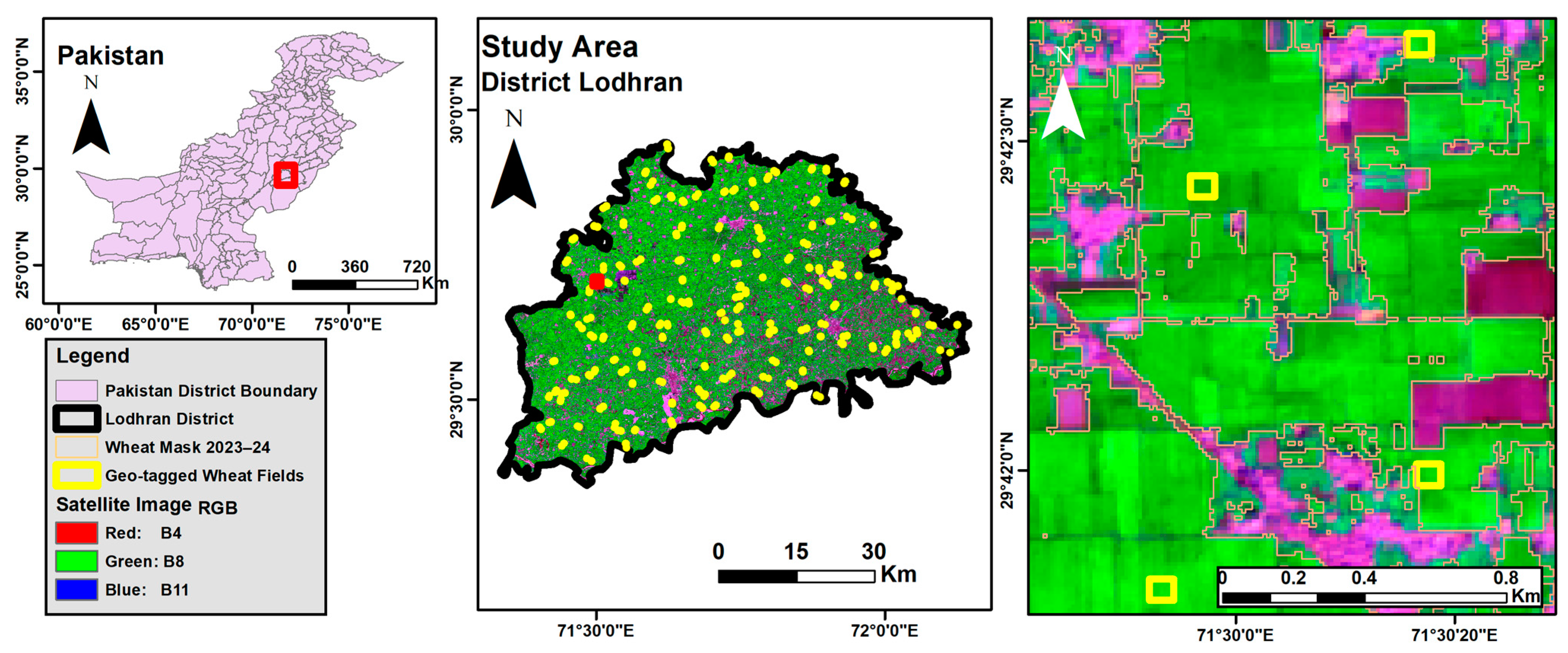
The overall workflow of this study consists of several steps, as outlined in Figure 1. After the study area description, the research methodology has two major components of data collection and preparation, followed by analysis methodology to identify the best-fit model for wheat crop trait mapping.

2.1. Study Area

This study was conducted in Lodhran district, Pakistan, which includes three tehsils: Dunyapur, Kehror Pacca, and Lodhran. Annually, more than 150,000 hectares of wheat are cultivated in this district. According to the Ministry of National Food Security and Research publication “CROPS AREA & PRODUCTION (District wise) 2022–2023,” approximately 155.4 thousand hectares of wheat were cultivated during 2022–2023 [37]. Multiple wheat fields within these tehsils were selected to conduct this study. The map of the Lodhran district with wheat mask 2023–2024 and selected fields are given in Figure 2.

2.2. Geo-Tagged Ground Data Information

The Punjab Agriculture Department collects geo-tagged information from selected farmers’ fields for their crop management practices and yield information. The department records detailed information on farm management practices, including fertilizer, irrigation, seed source, sowing date, plant population, soil type, and more. This geo-tagged information was obtained from the Punjab Agriculture Department to delineate selected farmers’ fields and simulate crop traits using APSIM NG based on sowing time, plant population, amount and time of fertilizer, and irrigation water application. The central point of each field was converted to a 60 × 60 m field boundary against the total field area of 4046.86 m² (one acre) to match the HLS pixel size of 30 m.

2.3. Agricultural Production Systems Simulator Next Generation (APSIM NG)

APSIM NG, an evolved version of APSIM classic 7.10, is a crop growth model that simulates wheat growth and development, like LAI or Above-Ground Biomass (AGB), on a daily time interval under principles of crop physiology based on weather and crop management information [23]. In this study, APSIM 2024.3.7412.0 was used for LAI simulation incorporating the weather and crop management information as input parameters. The weather data consisting of daily temperature (minimum and maximum), rainfall, and solar radiation from 2010 to 2024 were incorporated as the weather file, as crop growth, phenology, and yields are derived by weather variables [38]. The model has been validated for wheat crop in many regions worldwide, including Asia and Pakistan [39,40]. The geometric theory was employed to explore the relationship between LAI and the light extinction coefficient, which is a critical crop trait that influences daily radiation interception. This approach considers the impact of plant row spacing but does not differentiate between direct and diffuse light conditions or variations in radiation throughout the day [41].

2.4. Calibration of APSIM NG

LAI is directly simulated by most crop growth models and is often used for linkage or integration with other models, including RTM [14]. Other parameters like Cab, Cm and Cw, leaf structure (Ns), hotspot, etc. are derived parameters based on conversion formulas, mainly dependent on LAI [23]. Therefore, APSIM NG was calibrated specifically for LAI to ensure reliable estimation. The calibration steps as summarized in Figure 3 are described in the following subsections.

2.4.1. Ground Data Collection

A field campaign was conducted in selected wheat fields to measure LAI. Ground data of seven plots were collected for input information, sample wheat plants, and their count per m² to measure LAI for calibration of APSIM NG. Using this calibrated APSIM NG, LAI and other traits of 281 wheat fields were simulated without destructive sampling, along with saving time and resources. Resultantly, 1281 observations/samples of reflectance and traits were generated after data pre-processing and outlier removals for analysis.

2.4.2. Leaf Area Index Measurement

Due to the unavailability of leaf area meter and other measuring equipment in rural areas, ImageJ software (Ver 1.54i, Java 1.8 0_345) provides an effective way to measure LAI [42,43,44]. The number of plants per square meter was counted, and three plants were uprooted (destructive sampling) to measure leaf area from each selected farmer field. Leaves were detached from the plants and spread over white paper along with the scale to calibrate measurements in ImageJ software. Images were taken by camera and stored for further analysis in the software. During leaf area measurement, the scale was first calibrated in the software to measure the scale for number of pixels per cm. After image conversion to 8-bit and threshold setting, tracing was performed to measure all leaf areas. The average LAI of three plants was multiplied by the number of plants per square meter to obtain LAI.

2.4.3. APSIM NG Simulation

Before starting the APSIM NG simulation, the requisite model parameters, particularly for soil, weather, and wheat varieties, were calibrated in light of the literature relevant to APSIM wheat constants in Pakistan [39,40,45,46]. This calibration was particularly important for simulating wheat phenology under high-temperature conditions. Input parameters, including sowing time, plant population, and fertilizer and irrigation application, were collected from each farmer to have LAI and other relevant parameters on a daily basis.

2.4.4. Model Validation

A scatterplot was used to compare the measured LAI by ImageJ with the LAI simulated by APSIM NG on the date of sampling (14 January 2024) based on root mean square error (RMSE) and coefficient of determination (R²). The results were encouraging, with RMSEs of 0.42 and R² of 0.96, indicating that the APSIM NG model accurately simulated LAI for the selected field data.

2.4.5. Other Crop Trait Calculations

Other crop traits, such as Cab, Cm, and Cw, were calculated through transformation from output parameters of APSIM NG. The transformation from APSIM NG outputs to PROSAIL inputs was achieved for all requisite parameters, including these crop traits, through the formulas given in

Table 1. APSIM NG outputs to PROSAIL input transformation formula and data ranges for reflectance simulation.

Output Parameter (APSIM)	Variable Transformation Formula and Ranges Applied for PROSAIL Reflectance Simulation	Input Variable (PROSAIL)	Unit
SLA	Ns = (0.9 × SLA + 0.025)/(SLA − 0.1) [47] (1.0 to 2.1)	Leaf mesophyll structure (Ns)	Unitless
Zs, LAI total, LAI Dead	$\mathrm{Cw}=\left\{\begin{array}{c}0.000196\cdot Z_s+0.0298,if{f}_{dead}=0;\\ 0.0223\cdot \exp \left(-1.90\cdot f_{dead}\right),if{f}_{dead}>0\end{array}\right\}$[23] where f dead = LAI Dead/LAI Total (0.003829 to 0.027478)	Leaf water content (Cw)	g/cm2
LDW, LAI total,	Cm = 10−4 × LDW/LAI Total where LDW = 10 × LAITotal/SLA [23] (0.005025 to 0.007370)	Leaf dry matter content (Cm)	g/cm2
CNC, LAI total,	Cab = 26 × LNC [48] where LNC = CNC/LAI total (15.83 to 83.92)	Leaf Chlorophyll a and b content (Cab)	µg/cm2
	Car = 0.216 × Cab [48] (3.42 to 18.13)	Leaf carotenoid content (Car)	µg/cm2
LAI	Leaf Area Index (0.008 to 4.58)	LAI	-
LAI total,	hspot = a/LAI [49], where a is an empirical parameter considered as 0.5 (0.098 to 0.224)	Hot spot size parameter (hspot)	m/m1
/	Fixed ALA to 50° [23]	Average Leaf Angle	degree
/	Fixed Cant to 0 [23]	Leaf anthocyanin content (Cant)	µg/cm2
/	Fixed Cbrown to 0 [23]	Cbrown	Unitless
psoil	Fixed psoil to 1 [23]	Reflectance of soil as a libertarian surface	Unitless

SLA = Specific Leaf Area (cm²/mg¹), LDW = g/m².

with data ranges used for PROSAIL reflectance simulation.

2.5. Reflectance Data (RTM and HLS)

2.5.1. Radiative Transfer Model Reflectance

The PROSAIL-5B model was used that requires 14 input parameters, categorized into leaf properties, background soil properties, canopy architecture, and solar-object-sensor observation geometry. Its output includes the directional canopy reflectance across wavelength from 400 to 2500 nm at 1 nm interval.

In this study, the variables listed in Table 1 were used as input parameters for the PROSAIL-5B model to generate the reflectance. The Solar Zenith Angle (SZA), Viewing Zenith Angle (VZA), and Relative Azimuth Angle (RAA) were calculated from harmonized landsat-sentinel-2 (HLS) data. The average SZA, VZA, and RAA were calculated for available dates and farmer fields to be used as input variables in the PROSAIL-5B model.

PROSAIL simulated reflectance was converted to equivalent satellite reflectance datasets using the satellite sensor’s spectral response function (SRF) [50]. The HLS data reference the Operational Land Imager (OLI) spectral bandpasses for common and corresponding bands of Sentinel-2 and Landsat for HLS S30 and L30 products. The transformation of PROSAIL reflectance to equivalent OLI reflectance for crop trait retrieval was performed using the following equation [51]:

$$R_{rs}\left(ban{d}_i\right)={\displaystyle \frac{{\displaystyle {\int }_{{\lambda }_1}^{{\lambda }_2}{R}_{rs}\left(\lambda \right)SRF\left(\lambda \right)d\lambda }}{{\displaystyle {\int }_{{\lambda }_1}^{{\lambda }_2}SRF\left(\lambda \right)d\lambda }}}$$

(1)

where $i$ represents the band number of OLI; $\lambda$₁and $\lambda$₂ is the minimum and maximum wavelengths for ${band}_i$; and $R_{rs}\left(\lambda \right)$ and $SRF\left(\lambda \right)$ denote the PROSAIL simulated reflectance and OLI spectral response function, respectively, at wavelength $\lambda$. Seven common bands of the L30 and S30 products of HLS, as given in

Table 2. Spectral bands information of HLS.

Band Name	Wavelength (Micrometers)	HLS Band Code Name Landsat-8	HLS Band Code Name Sentienl-2
Coastal Aerosol	0.43–0.45	B01	B01
Blue	0.45–0.51	B02	B02
Green	0.53–0.59	B03	B03
Red	0.64–0.67	B04	B04
NIR Narrow	0.85–0.88	B05	B8A
SWIR 1	1.57–1.65	B06	B11
SWIR 2	2.11–2.29	B07	B12

, were selected to estimate the crop traits.

2.5.2. HLS Reflectance (Farmers’ Fields)

NASA initiated the Harmonized Landsat and Sentinel-2 (HLS) project to create a Virtual Constellation (VC) of surface reflectance data from the Operational Land Imager (OLI) on Landsat 8/9 (L30 product) and the Multi-Spectral Instrument (MSI) on Sentinel-2 (S30 product) [50]. The HLS products are generated using a series of algorithms designed to produce seamless data from both sensors, offering improved temporal coverage. In this study, HLS reflectance was processed from available cloud-free images within the active growth period of wheat crop (7 December 2023 to 15 March 2024). The reason for selecting this period was based on the long duration of wheat sowing (end of October to end of November) and start of wheat maturity (end of March). Due to extreme weather conditions during this year, no cloud-free images were available for Landsat and Sentinel-2 for the month of January 2024. Resultantly, the eight available cloud-free images during this period include two images of L30 product (7 December and 4 March) and six images of S30 product (16 and 21 December, 4, 14, and 24 February, and 15 March). Thus, the harmonization of two sensors provides more temporal coverage than a single senor. The average reflectance of each band was processed against the geo-tagged field boundaries of each sample. The common bands of L30 and S30 shown in above Table 2 were used to have consistent data and enhanced temporal coverage to explore the relationships between reflectance and crop traits.

2.5.3. Data Pre-Processing, Standardization, and Feature Selection

To ensure effective analysis of PROSAIL (RTM) as training data, pre-processing [52] and standardization [53] are essential to match and test with satellite-based reflectance (real-world scenarios). Therefore, pre-processing of PROSAIL-5B data was performed through normalization, transformation, and outlier removal. The compatibility between the simulated reflectance spectra from PROSAIL and HLS was assessed through Pearson’s correlation coefficient, with most bands having a strong correlation (r > 0.7). A linear transformation was applied to further align PROSAIL data with HLS data. Outliers were identified on the basis of residuals by calculating the difference between reflectance of two datasets for each band of the corresponding dates. Outliers were detected on the basis of threshold applied to these residuals. Standard deviation and interquartile range methods were applied by following the below equations.

$$Residual=X_{HLS}-X_{PROSAIL}$$

(2)

$$Residual\_outlier=\left\{Residual\right|Residual>\mu \_Residual+3\sigma \_ResidualorResidual<\mu \_Residual-3\sigma \_Residual\}$$

(3)

where μResidual is the mean of the residuals, and σResidual is the standard deviation of the residuals.

$$Residual\_outlier=\left\{Residual\right|Residual>Q\_3^Residual+1.5\ast IQR\_ResidualorResidual<Q\_1^Residual-1.5\ast IQR\_Residual\}$$

(4)

Moreover, feature selection on specific bands and selected dates was also evaluated to observe the accuracy improvement for PROSAIL model reflectance. The inclusion of vegetation indices (NDVI, NDWI EVI) effectively contributed to accuracy improvement [27]. Additionally, LAI has a parabolic nature, having values in descending order after reaching peak vegetative growth identical to the ascending pattern from sowing to peak vegetative growth. So, after maximum LAI or peak vegetative stage, there will be a higher probability of identical spectra by the PROSAIL model. Therefore, selection of suitable duration, particularly up to the peak of crop growth (up to 14 February), can further enhance the accuracy of the PROSAIL-to-HLS alignment.

2.6. Machine Learning Models

Machine learning models are widely applied in agriculture, not only for better understanding crop growth and development but also for developing novel and sustainable crop management practices [54]. Machine learning models are even now utilized for genome editing programs for accelerated crop improvement [54]. Numerous studies [23,26,55,56] have investigated machine learning models for different crop trait retrieval. Keeping in mind the literature and wide applicability of machine learning models, three models, Support Vector Machine (SVM), Random Forest (RF), and Extreme Gradient Boosting (XGBoost), were selected for retrieval of crop traits in this study.

2.6.1. Model Input and Output Parameters

In addition to the reflectance of the seven selected bands, indices like Normalized Difference Vegetation Index (NDVI), Normalized Difference Water Index (NDWI), and Enhanced Vegetation Index (EVI) were also included as input parameters. These indices are also linked to biophysical variables and used for crop growth monitoring and productivity assessment [57]. Thus, a total of 10 parameters (7 band reflectances and 3 indices) were used as input parameters to estimate four output parameters: LAI, Cab, Cm, and Cw. Analysis was performed on two datasets, given in

Table 3. Dataset information used in analyses.

Dataset Name	Dataset Composition	No. of Samples in Dataset	No. of Training and Test Samples
Dataset-1	PROSAIL Reflectance HLS Reflectance	PROSAIL = 1281 HLS = 1281	Training = 1281 Test = 1281
Dataset-2	HLS Reflectance	HLS = 1281	Training = 1010 (80%) Test = 271 (20%)

, to compare the predictive accuracy of crop trait estimation under two different scenarios. Dataset-1, presenting scenario one (simulated vs. satellite), consisted of full uniform PROSAIL-generated reflectance (1281) as the training dataset and HLS surface reflectance as the test dataset (1281). Under scenario two (satellite only), Dataset-2 (test data of scenario one) was prepared by splitting the HLS surface reflectance into 1010 training samples (80%) and 271 test samples (20%) as an alternate approach.

2.6.2. Model Optimization and Performance Analysis

After data pre-processing and normalization, the models were optimized using a grid search combined with cross-validation. Specifically, 5-fold cross-validation was found best for the RF and XGBoost models, and 10-fold cross-validation for the SVM model. Hyperparameter tuning of each model and each trait with relevant parameters is given as

Table 4. Hyperparameters for each model and trait.

Hyperparameters	Dataset-1 (PROSAIL-HLS)				Dataset-2 (HLS; 80:20)
	LAI	Cab	Cm	Cw	LAI	Cab	Cm	Cw
Random Forest
Max Depth	75	100	None	25	25	10	None	10
Min Sample Leaf	4	1	1	1	1	4	1	1
Min Sample Split	10	10	2	5	5	10	2	2
n-estimator	200	100	500	100	100	200	500	100
OOB Error	0.0049	0.4578	3.3 × 10−9	3.7 × 10−8	0.0448	7.613	4.8 × 10−9	6.6 × 10−7
Support Vector Machine
C	100	100	1	250	250	500	1	2000
Gamma	0.1	0.1	0.1	5.0	5.0	1	0.1	0.1
Kernel	rbf	rbf	rbf	rbf	rbf	rbf	rbf	rbf
Epsilon	0.05	0.001	0.1	0.001	0.05	0.05	0.1	0.001
Extreme Gradient Boost
Learning Rate	0.001	0.01	0.001	0.01	0.01	0.01	0.001	0.01
Max Depth	10	100	4	100	10	10	4	10
Regular Lambda	2.0	1.0	1.0	1.0	2.0	2.0	1.0	2.0
n-estimator	750	750	500	750	750	500	500	500

. This approach ensured robust and reliable performance evaluation, improving both predictive accuracy and generalizability. The RMSE, Mean Absolute Error (MAE), and R² metrics were used to evaluate the performance and accuracy of the models based on Dataset-1 and Dataset-2, given above in Table 3. Data consistency was maintained by using the same corresponding datasets for model testing.

3. Results

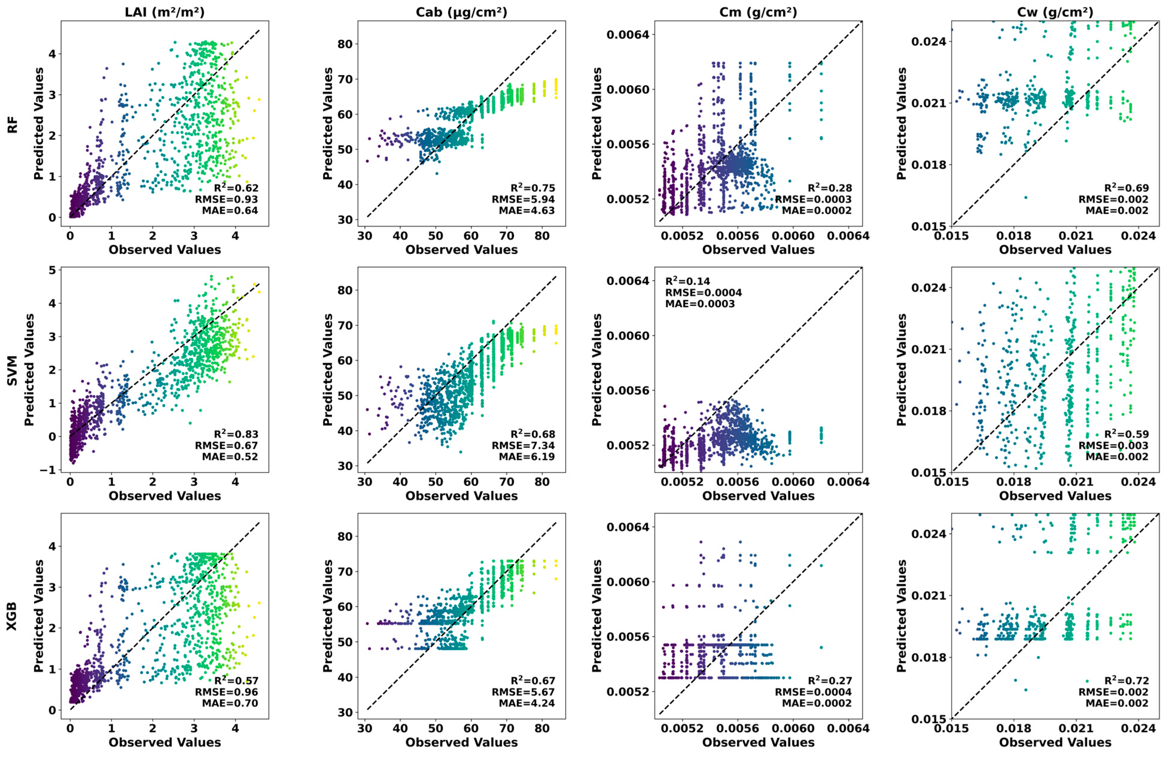
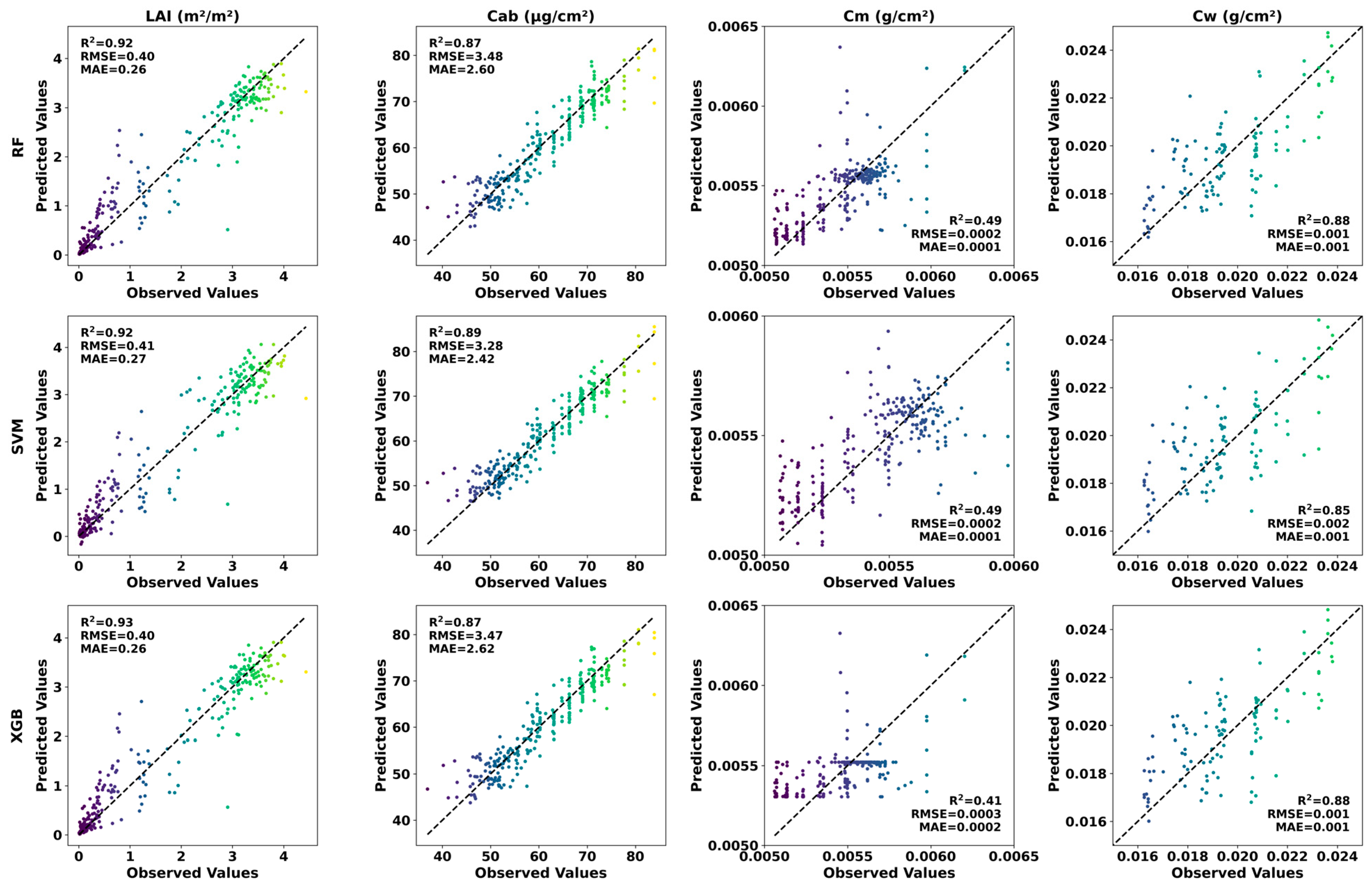
3.1. Model Performance

The performance of machine learning models is summarized in

Table 5. Machine learning model performance evaluation.

Data Type	Model	LAI			Cab (µg/cm2)			Cm (g/cm2)			Cw (g/cm2)
		RMSE	MAE	R2	RMSE	MAE	R2	RMSE	MAE	R2	RMSE	MAE	R2
Dataset-1	RF	0.93	0.64	0.62	5.94	4.63	0.75	0.0003	0.0002	0.28	0.002	0.002	0.69
	SVM	0.67	0.52	0.83	7.34	6.19	0.68	0.0004	0.0003	0.14	0.003	0.002	0.59
	XGBoost	0.96	0.70	0.57	5.66	4.23	0.67	0.0004	0.0002	0.27	0.002	0.002	0.72
Dataset-2	RF	0.40	0.26	0.92	3.48	2.60	0.87	0.0002	0.0001	0.49	0.001	0.001	0.88
	SVM	0.41	0.27	0.92	3.28	2.42	0.89	0.0002	0.0001	0.49	0.002	0.001	0.85
	XGBoost	0.40	0.26	0.93	3.47	2.62	0.87	0.0003	0.0002	0.41	0.001	0.001	0.88

as per the prescribed evaluation criteria for Dataset-1 and Dataset-2. The results indicate that SVM and XGBoost outperformed RF for LAI and Cab on both datasets. SVM predicted LAI with an RMSE of 0.67 and R² of 0.83 for Dataset-1, whereas XGBoost showed superior performance with an RMSE of 0.40 and R² of 0.93 for Dataset-2.

However, in the case of Cab, XGBoost performed best on Dataset-1 with an RMSE of 5.66 µg/cm², MAE of 4.23 µg/cm², and R² of 0.67, whereas SVM excelled on Dataset-2, with RMSE of 3.28 µg/cm², MAE of 2.42 µg/cm², and R² of 0.89. RF also performed well for Cab prediction on Dataset-1 and Dataset-2, as given in Table 5. RF performance on Dataset-2 is similar to XGBoost, with RMSE difference of 0.01 µg/cm². Figure 4 and Figure 5 illustrate the scatterplots for each model performance in estimating the crop traits for Dataset-1 and Dataset-2, respectively.

However, for predicting leaf dry matter content (Cm) and leaf water content (Cw), RF and XGBoost proved more reliable in explaining the variability and understanding relationships between variables from both datasets. RF achieved the best prediction for Cm, with RMSEs of 0.003 g/cm² and 0.002 g/cm², MAEs of 0.002 g/cm² and 0.001 g/cm², and R² of 0.28 and 0.49 on Dataset-1 and Dataset-2, respectively, followed by XGBoost on Dataset-1. SVM performed similar to RF for Cm on Dataset-2, as shown in Table 5. SVM, despite its good performance on LAI and Cab, was less effective for Cm and Cw on Dataset-1, as shown by its low values of evaluation criteria for Dataset-1 (Table 5). XGBoost performed better than others for Cw on both Datasets with RMSE of 0.002 and 0.001 g/cm², MAE of 0.002 and 0.001 g/cm² and R² of 0.72 and 0.88 for Dataset-1 and Dataset-2 respectively. RF also had equivalent performance to XGBoost in predicting Cw on Dataset-2. SVM showed less prediction accuracy compared to other models for Cw on both datasets (Table 5).

Figure 5 highlights the performance differences among the machine learning models in predicting crop traits against Dataset-1. The SVM model effectively predicted LAI values above 4, whereas other models were limited to predictions around 4 against the observed LAI values around 4.60. Similarly, SVM effectively captured the lower LAI values as compared to RF and XGBoost, whereas, in the case of Cab estimation for Dataset-1, XGBoost and RF remained efficient, particularly the XGBoost in the prediction of Cab values above 65 µg/cm². SVM underestimated Cab and remained within the lower ranges of below 50 µg/cm². RF successfully predicted Cm values above 0.0060 g/cm², aligning with the observed values up to 0.0073 g/cm², followed by XGBoost, while SVM was unable to predict values above 0.006 g/cm².

Regarding Cw, XGBoost demonstrated the highest prediction accuracy, particularly for values near the average. The prediction range centered around 0.02 g/cm², with good responsiveness to observed values ranging from 0.0019 to 0.0028 g/cm². However, RF performed better on Dataset-1 in predicting values within the same range as observed, closely matching XGBoost (Figure 4). Machine learning models showed potential for crop trait estimation but had limitations in capturing the full range of observed data for Dataset-1, particularly for Cm and Cw, having narrow variation ranges.

As shown in Figure 5 for Dataset-2, all machine learning models demonstrated a good fit with observed values for both LAI and Cab as compared to Dataset-1. The scatterplots for LAI indicated no significant difference in prediction accuracy among the models. XGBoost and RF demonstrated similar performances for both LAI and Cab. A similar consistent pattern was observed in scatterplots of Cab for all models, with small variations in RMSE of 3.28 to 3.48 µg/cm², MAE of 2.24 to 2.26 µg/cm², and similar R² of 0.87, depicting good response to data variance by all models.

In predicting Cm, the RF model performed best, closely followed by XGBoost, responding well to observed data. In contrast, the SVM model predicted values only below 0.006 g/cm² and struggled to capture the variance effectively, particularly for higher observed values. In the case of Cw, all models performed well, with the best one by XGBoost and RF (Figure 5). Among the models, there was a difference of 0.001 g/cm² RMSE and 0.03 R² between the top ones (XGBoost and RF) and the lower one (SVM). This shows that for Dataset-2, all models effectively responded to data variance for Cw.

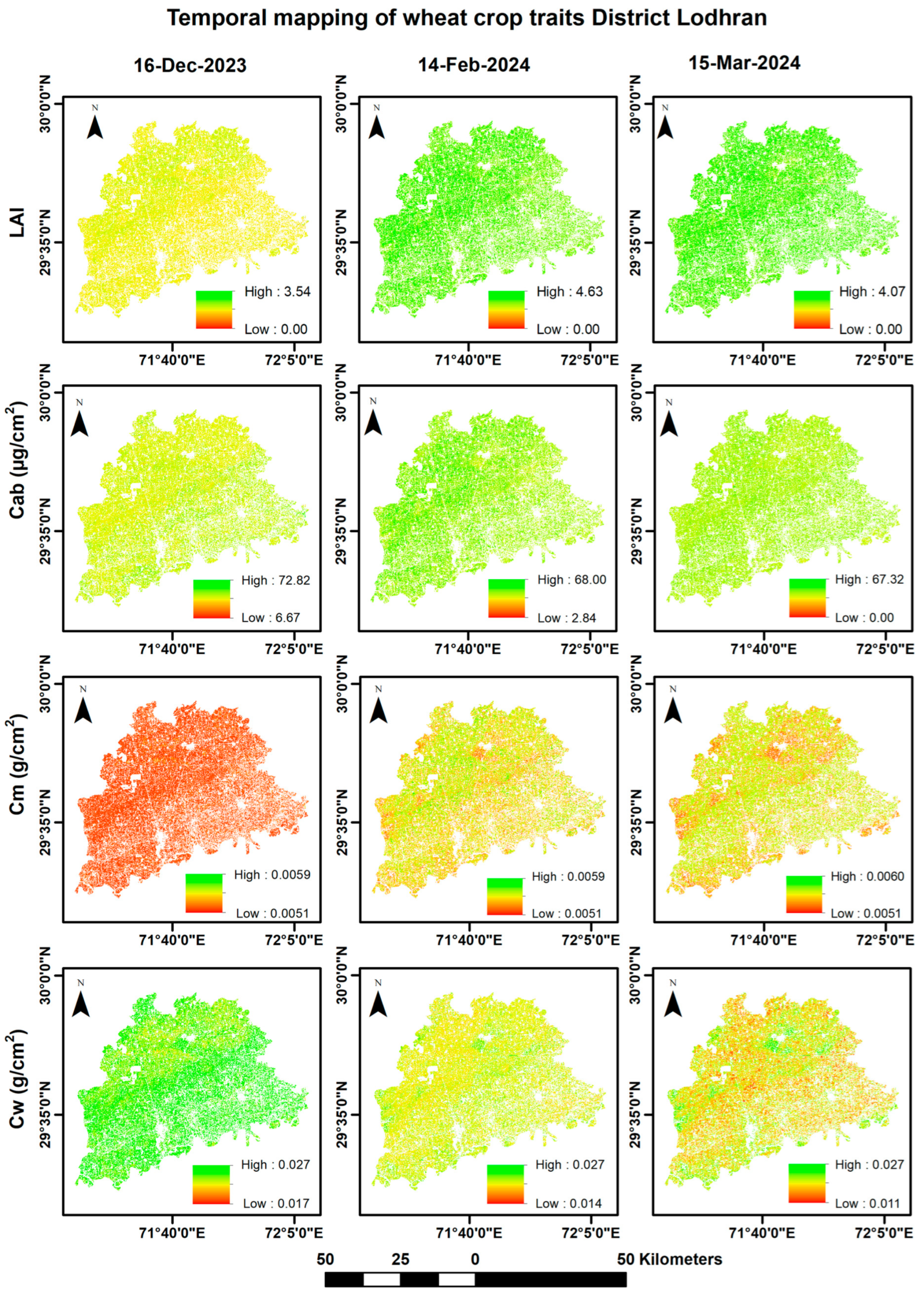
3.2. Wheat Trait Temporal Mapping

Given the superior performance of Dataset-2, the best performing models (XGBoost for LAI, SVM for Cab and RF for Cm and Cw) were applied to estimate wheat crop traits across the Lodhran district using satellite imagery. Among the available eight dates, three key dates were selected for mapping: 16 December (start of season), 14 February (mid-season), and 15 March (end of season). The selected dates are in line with wheat growth duration, having sowing in November and harvesting from the end of March [58]. Figure 6 presents the estimation maps of LAI, Cab, Cm, and Cw for the district on the given dates.

The LAI map for 16 December showed values given in Figure 6, with most pixels clustering around the average estimated value, accurately reflecting wheat growth during the initial period. By 14 February, the model predicted above-average values, with a peak LAI of 4.63, followed by a slight decrease to 4.07 on 15 March [59]. Cab displayed the highest prediction accuracy among wheat traits, tracking a clear decreasing trend consistent with wheat growth stages, mainly due to nutritional redistribution and crop maturity. The maximum Cab predicted on 16 December was gradually decreased on March 15 as shown in Figure 6, in line with wheat crop growth toward maturity [60]. Mapping Cm presented challenges due to narrow variations in observed data. The minimum and maximum values of Cm during the mapping period were 0.0051 and 0.0060, respectively. Most fields exhibited an average Cm value near the lower values, with limited areas showing an above-average Cm value. These values gradually increased as dry matter accumulated till peak vegetative growth stage [61]. Cw mapping was, however, better than Cm, with predicted values given in Figure 6. The gradual decrease in Cw corresponded to reduced moisture content, particularly by 15 March as the crop approaches maturity; otherwise, it adversely affects wheat crop yield [62].

4. Discussion

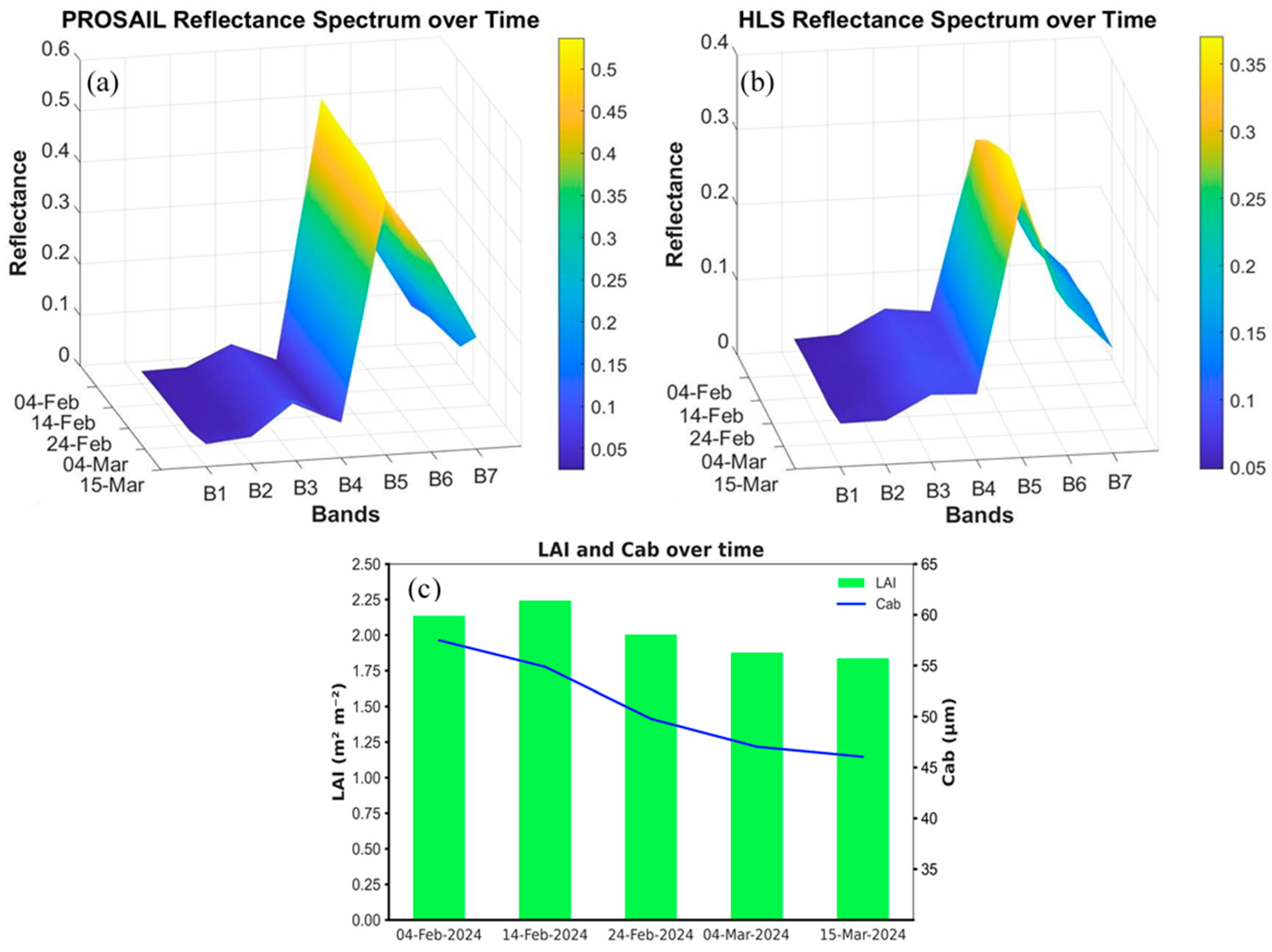
4.1. PROSAIL and HLS Reflectance

A satisfactory retrieval accuracy of crop traits based on reflectance from Dataset-1 demonstrates the potential of using PROSAIL outputs as training data coupled with the APSIM model. The advantage of this approach lies in the generation of uniform PROSAIL training sample for multiple traits rather than a biased and trait-specific sample selection [26]. Although Dataset-2 performed much better than Dataset-1, it requires field coordinates for reflectance extraction to build the training sample. The limitations in Dataset-1 are mainly attributed to generation of the same reflectance for different combinations of crop traits by the PROSAIL model [7,20,23]. But a comparative analysis of two datasets, named cdata and rdata, concluded that integration of CGM-RTM (cdata) outperformed rdata that were synthetic, generated using conventional random ranges and distributions of input parameters with the PROSAIL model alone. The study revealed that the cdata integration significantly outperformed rdata in both correlation coefficients (LAI = 1, Cm = 0.99, Cw = 0.95 for cdata vs. LAI = 0.99, Cm = 0.74, Cw = 0.64 for rdata) and RMSE values (LAI = 0.04, Cm = 0.00013, Cw = 0.0015 for cdata vs. LAI = 0.17, Cm = 0.00084, Cw = 0.0093 for rdata). These findings underscore the superior predictive accuracy and reduced error of the APSIM-PROSAIL integrated approach compared to the standalone PROSAIL model.

Secondly, most RTM-based studies used trait-specific selected reflectance data due to RTM limitations [7,26,63]. This study used full PROSAIL-generated training data for all traits without any biased sample selection addressing the RTM limitations. It is hard to find studies that used all RTM spectra as training data, indicating RTM alone has a limitation in accurately predicting crop traits. The same is also described by these studies [7,26,63] and validated by Chen et al. [23]. The RTM-CGM integration due to biological constraints not only improves retrieval accuracy but also enables joint estimation of multiple traits, particularly the Cm and Cw, as reported in [23] as well. These traits (Cm and Cw) have limited studies with narrow data variation ranges, making their prediction challenging [14]. The effectiveness of this proposed approach can also be supported by the many studies given in

Table 6. Performance of RTM standalone estimation for Cw and Cm.

Crop Trait	Crop	Range of R2/r and RMSE Across Techniques		Reference
		R2/r	RMSE (g/cm2)
Cw	Wheat	r = 0.17–0.74	0.005–0.009	[64]
* CWC	Wheat	R2 = 0.37–0.50	0.0096 to 0.027	[52]
Cw	Wheat and others	R2 = 0.10–0.30	0.019–0.023	[65]
Cm	Wheat	r = 0.36–0.69	0.0005–0.0006	[66]
Cm	Wheat	R2 = 0.00	0.0018	[67]
Cm	Multiple (herbaceous 45 plants)	R2 = 0.01–0.30	0.0015–0.01	[68]

* Canopy Water Content.

, having performance limitations for Cm and Cw with the advantage of uniform full PROSAIL-generated training data for the estimation of multiple crop traits.

Feature importance in the data analysis was in line with the general characteristics of the satellite data bands and indices. Overall, B5, B3, B6, NDWI, EVI, and NDVI have high importance in the prediction of crop traits [69,70,71]. A small variation in their importance is related to crop traits. For example, for LAI and Cab, B5 have the highest importance, followed by NDVI for Cm and NDWI and B6 for Cw. This is because of band sensitivity (B6 sensitive to moisture) and specific features of the indices (NDVI and EVI sensitive to biomass or LAI) to respond to crop characteristics [72,73].

In analyzing data for individual farmers, it was observed that variations in PROSAIL inter and intra bands is non-significant, particularly in consecutive dates of 14 to 24 February and 4 to 15 March over time as compared to HLS reflectance, particularly the NIR band (Band 5). The decreasing trend in LAI and Cab over time was observed (Figure 7). However, the response of PROSAIL reflectance was less pronounced compared to HLS reflectance during this period. Consequently, it is recommended to use higher intervals or distinct variations in farm management practices and field information for PROSAIL spectra generation using APSIM or other crop growth models to avoid producing similar spectra for different trait values.

Satellite reflectance through geo-tagged field data collection may provide better predictions for crop trait estimation, as it not only accounts for crop management operations but also their impact on crop growth and development. Currently, many techniques, like integration of CGM (APSIM), to standardize PROSAIL reflectance are under investigation to improve crop trait estimation [23]. The need for standardizing the PROSAIL model arises due to its tendency to overestimate reflectance [74]. In previous studies, the addition of noise to PROSAIL data used for training canopy water content [52], as well as coupling the PROSAIL model with the unified linearized vector radiative transfer model (UNL-VRTM) for LAI and Cab, proved effective in enhancing accuracy [53]. Similar is the scenario in our study, where APSIM-integration-based PROSAIL reflectance followed by data standardization through linear transformation and suitable duration selection allowed for satisfactory retrieval of multiple crop traits (LAI, Cab, Cm, and Cw) using PROSAIL as training data and HLS as test data (Dataset-1). These findings not only validated the technical innovation from previous research [23], but also demonstrated improved retrieval accuracy for wheat crop traits, particularly Cm and Cw.

Thus, an effective approach for generating PROSAIL reflectance is through CGM integration, which creates unbiased training data for multiple crop traits, avoiding trait-specific sample selection. Satellite-based reflectance offers a promising alternative in the recent era of artificial intelligence, where delineation of functional field boundaries for agricultural operations is under investigation through various models [75,76]. This provides the opportunity to integrate field information from the APSIM model with field-based reflectance, enabling more reliable crop trait estimation.

4.2. Model Performance

Our results showed that XGBoost overall demonstrated superior performance for multiple traits on both datasets, demonstrating its robustness to handle sparse and noisy data. Reflectance data is often noisy due to variations in cloud cover, sunlight, and atmospheric conditions, but XGBoost is suitable for such kinds of data and captures variations in reflectance and indices [77]. On an individual trait basis, SVM performed well for LAI (RMSE = 0.67, and R² = 0.83) on Dataset-1, while the XGBoost excelled on Dataset-2 (RMSE = 0.40 and R² = 0.93). Similarly, for other traits, models generally performed better on Dataset-2 compared to Dataset-1. Better performance of SVM for LAI on Dataset-1 and for Cab on Dataset-2 indicates model strength to find relationships between the reflectance and these two traits. These traits exhibit higher values and greater variability, demonstrating the SVM’s ability to handle large margins and complex data distributions.

In contrast, RF and XGBoost outperformed SVM in predicting Cm and Cw. These traits were characterized by lower values and narrow variations, indicating the robustness of the ensemble-learning approach and effectiveness in capturing the subtle patterns within these more constrained datasets [78]. The ability of average multiple-decision trees by RF and sequential trees building approach by XGBoost reduces variance and enhances accuracy for traits, even with minimal variation in these crop traits [79]. This performance difference highlights the importance of selecting appropriate algorithms based on the specific characteristics and variability of the target traits and datasets. SVM, however, struggled with predicting Cm and Cw, mainly due to the majority of samples clustering near the average and narrow variation range, causing overlapping and noisy data, which make prediction challenging for SVM [80].

Moreover, Dataset-1 showed greater retrieval differences among machine learning models, describing moderate relations among the variables. For example, SVM (the best model for LAI estimation) has an RMSE of 0.67 (R² = 0.83), and XGBoost has an RMSE of 0.96 (R² = 0.57). However, Dataset-2 exhibited less discrepancy among models for estimation of all traits, indicating stronger relations among variables to have consistency and reliability in crop trait estimation. In contrast to Dataset-1, Dataset-2 has an RMSE of 0.40 (R² = 0.93), with XGBoost (best model) compared to the SVM model RMSE of 0.41 (R² = 0.92). Although satellite-based reflectance from geo-tagged field boundaries is more accurate, PROSAIL-generated reflectance data also showed satisfactory results in line with previous studies [23,52,53]. This approach provides an opportunity for applicability under limited ground information scenarios, particularly at the start of the season, offering advantages in labor, cost, and non-destructive crop trait measurement through integration with the APSIM model.

4.3. Traits Performance

Among the crop traits, Cab has the highest predictive accuracy, followed by LAI. This high accuracy for Cab is attributed to its strong relation to green bands and weak to red bands, as reflectance gradually decreases with increasing Cab [81]. Moreover, studies also show that Cab and LAI are sensitive to specific bands, enhancing their prediction accuracy compared to Cm and Cw [53]. Therefore, these traits not only have low RMSE (0.4 and 0.67 for LAI; 3.28 and 5.66 µg/cm² for Cab), but have higher R² values for Dataset-1 and 2 (0.83, 0.92 for LAI; 0.67, 0.89 for Cab).

The simulations showed that Cw is sensitive to the short-wave infrared region, with the best range of 1.391 to 1.830 µm for wheat [82]. However, the narrow variation range makes it challenging to establish a strong prediction relationship but efficient than Cm [14]. Although Cm is sensitive to the NIR band, its contribution is inversely related to LAI, making prediction more challenging, particularly for Dataset-1 [81]. The reason behind this challenge arises from the narrow numerical range and low variation in these traits. Previous studies have similarly shown that limited ranges and variations result in weak correlations and unreliable estimations for both Cm and Cw [14,20,23,83].

4.4. Temporal Mapping of Crop Traits

The temporal maps generated for each trait aligned well with wheat behavior and its physiology. The LAI map for 16 December showed lower values, corresponding to the early growth stage, which increased during February, reflecting the peak growth period. In contrast, Cab values were higher in December and gradually decreased over time, which corresponds to the physiological shift in wheat, where nitrogen and chlorophyll content in the leaves diminishes as nutrients are redirected toward grain formation and production [60].

Cm and Cw, however, remain challenging traits to estimate, as confirmed by multiple studies, mainly due to their lower numerical ranges and narrow variations [14,20,23,83]. Cm exhibited an upward trend, particularly at wheat maturity on 15 March, though its values generally remained within the low to medium range. Cw mapping, in contrast, was better than Cm. Between 16 December and 14 February, the growth of wheat exhibited higher Cw values, indicating more green fields with higher water content due to the increased size and weight of wheat leaves. However, from 14 February to 15 March, Cw showed a downward trend across a large area, indicating the crop development toward maturity. This decline is likely due to reduced leaf growth, limited irrigation, and increased evapotranspiration during March [26].

In summary, these temporal maps provide a comprehensive overview of the spatial and temporal dynamics of key wheat traits. The LAI maps indicate robust leaf growth, with variations across the three dates. The Cab maps reveal moderate chlorophyll content, with a slight decline as the crop matures. The Cm maps indicate consistent leaf mass per area with minor fluctuations, while the Cw maps reveal significant variations in leaf water content, highlighting areas of water stress and recovery. Overall, these maps are critical for monitoring crop health and guiding agricultural practices in the district.

4.5. Limitations of This Study

The unavailability of satellite data due to weather constraints between 21 December and 4 February resulted in a gap and non-uniform crop growth profile. The majority of farmers’ fields have their maximum LAI in late January, which was not taken into consideration due to the unavailability of satellite data. The use of harmonized satellite data or synthetic aperture radar (SAR), like Sentinel-1, can help to overcome this limitation. Additionally, the wheat mask used for temporal mapping, though satisfactory in accuracy, still has the possibility of inaccuracy due to classification limitation. Thus, the potential presence of other crops, particularly of fodders, cannot be ruled out. This presence of other crops may have an impact on mapping of crop traits due to variation in reflectance from other crops causing a change in high or lower range of wheat crop traits. Advancement in crop discrimination techniques can effectively reduce this error.

5. Conclusions

This study demonstrated the effectiveness of integrating the APSIM NG with the PROSAIL model to predict multiple crop traits from uniform spectra without any biased sample selection. The integration of crop growth models enables the generation of realistic trait combination-based spectra instead of random combinations that may not exist, particularly in crop physiology. XGBoost and SVM performed well in estimating LAI (RMSE = 0.4, R² = 0.93) and Cab (RMSE = 3.28 µg/cm², R² = 0.89), whereas RF showed superior performance for Cm (RMSE = 0.0002 g/cm², R² = 0.49) and Cw (RMSE = 0.001 g/cm², R² = 0.88) estimation. In terms of reflectance data type, HLS performed consistently and reliably across all machine learning models, albeit with some variations. This APSIM-PROSAIL integration offers significant advantages in reducing labor, cost, and crop damage by avoiding destructive sampling techniques at various growth stages, with estimation of multiple traits through an interconversion formula used for PROSAIL input parameters. Although PROSAIL combined with HLS has the low performance than HLS alone, it still performs within acceptable limits, providing a viable option for training data under limited field information.

These integrated approaches with new technological advancements in CGM or RTM can lead to highly reliable prescription maps, which are valuable tools for effective decision-making in precision agriculture. The synergistic framework used in this study enables operational temporal mapping of LAI, Cab, Cm, and Cw for large wheat areas and can also be effective for other crops, with the advantages of inclusive coverage of field realities, farm activities, and their impact on crop growth. These crop traits integrally linked to constitute crop production; thus, they can be effective in crop yield modeling, damage assessment, or crop insurance and other relief measures, ultimately contributing to timely decision-making to assure food security.

Among traits, LAI is vital, as crop health and yield are not only directly linked to it but other traits also depend on it because it is an integral part of most transformational formulas. Additionally, reflectance from various bands, particularly of near-infrared and red, is also influenced by LAI. Moreover, future endeavors are focusing toward reliable estimation of LAI and other traits using remote sensing data. This underscores LAI as a key parameter for research involving reflectance and trait prediction across different crops and regions. Hybrid models in combination with active learning strategies also represent another avenue for enhancing the reliable prediction of these traits. Thus, future investigations should explore innovations like CGM integration for reliable LAI and/or other trait estimation and/or PROSAIL data standardization to further improve accuracy through training data and advanced machine learning models from the start of crop season for temporal mapping.

References

1. Clark, M.; Tilman, D. Comparative Analysis of Environmental Impacts of Agricultural Production Systems, Agricultural Input Efficiency, and Food Choice. Environ. Res. Lett. 2017, 12, 064016. [Google Scholar] [CrossRef]
2. De los Santos-Montero, L.A.; Bravo-Ureta, B.E.; von Cramon-Taubadel, S.; Hasiner, E. The Performance of Natural Resource Management Interventions in Agriculture: Evidence from Alternative Meta-Regression Analyses. Ecol. Econ. 2020, 171, 106605. [Google Scholar] [CrossRef]
3. Kganyago, M.; Mhangara, P.; Adjorlolo, C. Estimating Crop Biophysical Parameters Using Machine Learning Algorithms and Sentinel-2 Imagery. Remote Sens. 2021, 13, 4314. [Google Scholar] [CrossRef]
4. van Dijk, M.; Morley, T.; Rau, M.L.; Saghai, Y. A Meta-Analysis of Projected Global Food Demand and Population at Risk of Hunger for the Period 2010–2050. Nat. Food 2021, 2, 494–501. [Google Scholar] [CrossRef] [PubMed]
5. Tilman, D.; Balzer, C.; Hill, J.; Befort, B.L. Global Food Demand and the Sustainable Intensification of Agriculture. Proc. Natl. Acad. Sci. USA 2011, 108, 20260–20264. [Google Scholar] [CrossRef]
6. Croce, R.; Carmo-Silva, E.; Cho, Y.B.; Ermakova, M.; Harbinson, J.; Lawson, T.; McCormick, A.J.; Niyogi, K.K.; Ort, D.R.; Patel-Tupper, D.; et al. Perspectives on Improving Photosynthesis to Increase Crop Yield. Plant Cell 2024, 36, 3944–3973. [Google Scholar] [CrossRef]
7. Abdelbaki, A.; Schlerf, M.; Retzlaff, R.; Machwitz, M.; Verrelst, J.; Udelhoven, T. Comparison of Crop Trait Retrieval Strategies Using UAV-Based VNIR Hyperspectral Imaging. Remote Sens. 2021, 13, 1748. [Google Scholar] [CrossRef]
8. Lu, N.; Wang, W.; Zhang, Q.; Li, D.; Yao, X.; Tian, Y.; Zhu, Y.; Cao, W.; Baret, F.; Liu, S.; et al. Estimation of Nitrogen Nutrition Status in Winter Wheat From Unmanned Aerial Vehicle Based Multi-Angular Multispectral Imagery. Front. Plant Sci. 2019, 10, 1601. [Google Scholar] [CrossRef]
9. Murchie, E.H.; Burgess, A.J. Casting Light on the Architecture of Crop Yield. Crop Environ. 2022, 1, 74–85. [Google Scholar] [CrossRef]
10. Wang, Y.; Yin, Y. Agriculture in Silico: Perspectives on Radiative Transfer Optimization Using Vegetation Modeling. Crop Environ. 2023, 2, 175–183. [Google Scholar] [CrossRef]
11. Walker, B.J.; Drewry, D.T.; Slattery, R.A.; VanLoocke, A.; Cho, Y.B.; Ort, D.R. Chlorophyll Can Be Reduced in Crop Canopies with Little Penalty to Photosynthesis. Plant Physiol. 2018, 176, 1215–1232. [Google Scholar] [CrossRef] [PubMed]
12. Iwahashi, Y.; Sigit, G.; Utoyo, B.; Lubis, I.; Junaedi, A.; Trisasongko, B.H.; Wijaya, I.M.A.S.; Maki, M.; Hongo, C.; Homma, K. Drought Damage Assessment for Crop Insurance Based on Vegetation Index by Unmanned Aerial Vehicle (UAV) Multispectral Images of Paddy Fields in Indonesia. Agriculture 2022, 13, 113. [Google Scholar] [CrossRef]
13. Vollmer, J.; Johnson, B.L.; Deckard, E.L.; Rahman, M. Evaluation of Simulated Hail Damage on Seed Yield and Agronomic Traits in Canola (Brassica Napus L.). Can. J. Plant Sci. 2020, 100, 597–608. [Google Scholar] [CrossRef]
14. Ishaq, R.A.F.; Zhou, G.; Tian, C.; Tan, Y.; Jing, G.; Jiang, H. Obaid-ur-Rehman A Systematic Review of Radiative Transfer Models for Crop Yield Prediction and Crop Traits Retrieval. Remote Sens. 2024, 16, 121. [Google Scholar] [CrossRef]
15. Verrelst, J.; Malenovský, Z.; Van der Tol, C.; Camps-Valls, G.; Gastellu-Etchegorry, J.P.; Lewis, P.; North, P.; Moreno, J. Quantifying Vegetation Biophysical Variables from Imaging Spectroscopy Data: A Review on Retrieval Methods. Surv. Geophys. 2019, 40, 589–629. [Google Scholar] [CrossRef]
16. Gewali, U.B.; Monteiro, S.T.; Saber, E. Gaussian Processes for Vegetation Parameter Estimation from Hyperspectral Data with Limited Ground Truth. Remote Sens. 2019, 11, 1614. [Google Scholar] [CrossRef]
17. Ali, A.M.; Darvishzadeh, R.; Skidmore, A.; Gara, T.W.; Heurich, M. Machine Learning Methods’ Performance in Radiative Transfer Model Inversion to Retrieve Plant Traits from Sentinel-2 Data of a Mixed Mountain Forest. Int. J. Digit. Earth 2021, 14, 106–120. [Google Scholar] [CrossRef]
18. Jacquemoud, S.; Verhoef, W.; Baret, F.; Bacour, C.; Zarco-Tejada, P.J.; Asner, G.P.; François, C.; Ustin, S.L. PROSPECT + SAIL Models: A Review of Use for Vegetation Characterization. Remote Sens. Environ. 2009, 113, S56–S66. [Google Scholar] [CrossRef]
19. Zhou, G.; Niu, C.; Xu, W.; Yang, W.; Wang, J.; Zhao, H. Canopy Modeling of Aquatic Vegetation: A Radiative Transfer Approach. Remote Sens. Environ. 2015, 163, 186–205. [Google Scholar] [CrossRef]
20. Zhang, L.; Jia, M.; Guo, X.; Zhang, L.; Wang, M.; Wang, W. Mapping Mangrove Functional Traits from Sentinel-2 Imagery Based on Hybrid Models Coupled with Active Learning Strategies International Journal of Applied Earth Observation and Geoinformation Mapping Mangrove Functional Traits from Sentinel-2 Imagery Base. Int. J. Appl. Earth Obs. Geoinf. 2024, 130, 103905. [Google Scholar] [CrossRef]
21. Abdelbaki, A.; Schlerf, M.; Verhoef, W.; Udelhoven, T. Introduction of Variable Correlation for the Improved Retrieval of Crop Traits Using Canopy Reflectance Model Inversion. Remote Sens. 2019, 11, 2681. [Google Scholar] [CrossRef]
22. Quan, X.; He, B.; Li, X. A Bayesian Network-Based Method to Alleviate the Ill-Posed Inverse Problem: A Case Study on Leaf Area Index and Canopy Water Content Retrieval. IEEE Trans. Geosci. Remote Sens. 2015, 53, 6507–6517. [Google Scholar] [CrossRef]
23. Chen, Q.; Zheng, B.; Chen, T.; Chapman, S.C. Integrating a Crop Growth Model and Radiative Transfer Model to Improve Estimation of Crop Traits Based on Deep Learning. J. Exp. Bot. 2022, 73, 6558–6574. [Google Scholar] [CrossRef] [PubMed]
24. Li, Z.; Li, Z.; Fairbairn, D.; Li, N.; Xu, B.; Feng, H.; Yang, G. Multi-LUTs Method for Canopy Nitrogen Density Estimation in Winter Wheat by Field and UAV Hyperspectral. Comput. Electron. Agric. 2019, 162, 174–182. [Google Scholar] [CrossRef]
25. De Grave, C.; Verrelst, J.; Morcillo-Pallarés, P.; Pipia, L.; Rivera-Caicedo, J.P.; Amin, E.; Belda, S.; Moreno, J. Quantifying Vegetation Biophysical Variables from the Sentinel-3/FLEX Tandem Mission: Evaluation of the Synergy of OLCI and FLORIS Data Sources. Remote Sens. Environ. 2020, 251, 112101. [Google Scholar] [CrossRef] [PubMed]
26. Caballero, G.; Pezzola, A.; Winschel, C.; Casella, A.; Sanchez Angonova, P.; Rivera-Caicedo, J.P.; Berger, K.; Verrelst, J.; Delegido, J. Seasonal Mapping of Irrigated Winter Wheat Traits in Argentina with a Hybrid Retrieval Workflow Using Sentinel-2 Imagery. Remote Sens. 2022, 14, 4531. [Google Scholar] [CrossRef] [PubMed]
27. Jamali, M.; Soufizadeh, S.; Yeganeh, B.; Emam, Y. Wheat Leaf Traits Monitoring Based on Machine Learning Algorithms and High-Resolution Satellite Imagery. Ecol. Inform. 2023, 74, 101967. [Google Scholar] [CrossRef]
28. Luo, S.; He, Y.; Li, Q.; Jiao, W.; Zhu, Y.; Zhao, X. Nondestructive Estimation of Potato Yield Using Relative Variables Derived from Multi-Period LAI and Hyperspectral Data Based on Weighted Growth Stage. Plant Methods 2020, 16, 1–14. [Google Scholar] [CrossRef]
29. Danner, M.; Berger, K.; Wocher, M.; Mauser, W.; Hank, T. Efficient RTM-Based Training of Machine Learning Regression Algorithms to Quantify Biophysical & Biochemical Traits of Agricultural Crops. ISPRS J. Photogramm. Remote Sens. 2021, 173, 278–296. [Google Scholar] [CrossRef]
30. Zhang, Y.; Yang, J.; Liu, X.; Du, L.; Shi, S.; Sun, J.; Chen, B. Estimation of Multi-Species Leaf Area Index Based on Chinese GF-1 Satellite Data Using Look-up Table and Gaussian Process Regression Methods. Sensors 2020, 20, 2460. [Google Scholar] [CrossRef]
31. Kganyago, M.; Adjorlolo, C.; Mhangara, P. Exploring Transferable Techniques to Retrieve Crop Biophysical and Biochemical Variables Using Sentinel-2 Data. Remote Sens. 2022, 14, 3968. [Google Scholar] [CrossRef]
32. Ahmed, M.S.; Tazwar, M.T.; Khan, H.; Roy, S.; Iqbal, J.; Rabiul Alam, M.G.; Hassan, M.R.; Hassan, M.M. Yield Response of Different Rice Ecotypes to Meteorological, Agro-Chemical, and Soil Physiographic Factors for Interpretable Precision Agriculture Using Extreme Gradient Boosting and Support Vector Regression. Complexity 2022, 2022, 5305353. [Google Scholar] [CrossRef]
33. Chergui, N.; Kechadi, M.T. Data Analytics for Crop Management: A Big Data View. J. Big Data 2022, 9, 123. [Google Scholar] [CrossRef]
34. Chapagain, R.; Remenyi, T.A.; Harris, R.M.B.; Mohammed, C.L.; Huth, N.; Wallach, D.; Rezaei, E.E.; Ojeda, J.J. Decomposing Crop Model Uncertainty: A Systematic Review. Field Crops Res. 2022, 279, 108448. [Google Scholar] [CrossRef]
35. Pasqualotto, N.; D’Urso, G.; Bolognesi, S.F.; Belfiore, O.R.; Van Wittenberghe, S.; Delegido, J.; Pezzola, A.; Winschel, C.; Moreno, J. Retrieval of Evapotranspiration from Sentinel-2: Comparison of Vegetation Indices, Semi-Empirical Models and SNAP Biophysical Processor Approach. Agronomy 2019, 9, 663. [Google Scholar] [CrossRef]
36. Amin, E.; Verrelst, J.; Rivera-Caicedo, J.P.; Pipia, L.; Ruiz-Verdú, A.; Moreno, J. Prototyping Sentinel-2 Green LAI and Brown LAI Products for Cropland Monitoring. Remote Sens. Environ. 2021, 255, 112168. [Google Scholar] [CrossRef]
37. Government of Pakistan. Crops Area & Production (District Wise) 2022–2023; Ministry of National Food Security and Research (Economic Wing): Islamabad, Pakistan, 2024.
38. Togliatti, K.; Archontoulis, S.V.; Dietzel, R.; Puntel, L.; VanLoocke, A. How Does Inclusion of Weather Forecasting Impact In-Season Crop Model Predictions? Field Crops Res. 2017, 214, 261–272. [Google Scholar] [CrossRef]
39. Gaydon, D.S.; Balwinder-Singh, J.; Wang, E.; Poulton, P.L.; Ahmad, B.; Ahmed, F.; Akhter, S.; Ali, I.; Amarasingha, R.; Chaki, A.K.; et al. Evaluation of the APSIM Model in Cropping Systems of Asia. Field Crops Res. 2017, 204, 52–75. [Google Scholar] [CrossRef]
40. Shahid, M.R.; Wakeel, A.; Ullah, M.S.; Gaydon, D.S. Identifying Changes to Key APSIM-Wheat Constants to Sensibly Simulate High Temperature Crop Response in Pakistan. Field Crops Res. 2024, 307, 109265. [Google Scholar] [CrossRef]
41. Holzworth, D.; Huth, N.I.; Fainges, J.; Brown, H.; Zurcher, E.; Cichota, R.; Verrall, S.; Herrmann, N.I.; Zheng, B.; Snow, V. APSIM Next Generation: Overcoming Challenges in Modernising a Farming Systems Model. Environ. Model. Softw. 2018, 103, 43–51. [Google Scholar] [CrossRef]
42. Martin, T.N.; Fipke, G.M.; Winck, J.E.M.; Marchese, J.A. ImageJ Software as an Alternative Method for Estimating Leaf Area in Oats. Acta Agron. 2020, 69, 162–169. [Google Scholar] [CrossRef]
43. Easlon, H.M.; Bloom, A.J. Easy Leaf Area: Automated Digital Image Analysis for Rapid and Accurate Measurement of Leaf Area. Appl. Plant Sci. 2014, 2, 2–5. [Google Scholar] [CrossRef] [PubMed]
44. Singh Negi, N.; Singh, M. An Image Analysis Based System (Image J) for Determination of Leaf Area in Seven Chrysanthemum Varieties. Pharma Innov. J. 2023, 12, 2275–2281. [Google Scholar]
45. Hussain, J.; Khaliq, T.; Ahmad, A.; Akhtar, J. Performance of Four Crop Model for Simulations of Wheat Phenology, Leaf Growth, Biomass and Yield across Planting Dates. PLoS ONE 2018, 13, e0197546. [Google Scholar] [CrossRef] [PubMed]
46. Azmat, M.; Ilyas, F.; Sarwar, A.; Huggel, C.; Vaghefi, S.A.; Hui, T.; Qamar, M.U.; Bilal, M.; Ahmed, Z. Impacts of Climate Change on Wheat Phenology and Yield in Indus Basin, Pakistan. Sci. Total Environ. 2021, 790, 148221. [Google Scholar] [CrossRef]
47. Jacquemoud, S.; Baret, F. PROSPECT: A Model of Leaf Optical Properties Spectra. Remote Sens. Environ. 1990, 34, 75–91. [Google Scholar] [CrossRef]
48. Yang, G.; Zhao, C.; Pu, R.; Feng, H.; Li, Z.; Li, H.; Sun, C. Leaf Nitrogen Spectral Reflectance Model of Winter Wheat (Triticum aestivum) Based on PROSPECT: Simulation and Inversion. J. Appl. Remote Sens. 2015, 9, 095976. [Google Scholar] [CrossRef]
49. Verhoef, W.; Bach, H. Simulation of Hyperspectral and Directional Radiance Images Using Coupled Biophysical and Atmospheric Radiative Transfer Models. Remote Sens. Environ. 2003, 87, 23–41. [Google Scholar] [CrossRef]
50. Claverie, M.; Ju, J.; Masek, J.G.; Dungan, J.L.; Vermote, E.F.; Roger, J.C.; Skakun, S.V.; Justice, C. The Harmonized Landsat and Sentinel-2 Surface Reflectance Data Set. Remote Sens. Environ. 2018, 219, 145–161. [Google Scholar] [CrossRef]
51. Ali, A.; Zhou, G.; Pablo Antezana Lopez, F.; Xu, C.; Jing, G.; Tan, Y. Deep Learning for Water Quality Multivariate Assessment in Inland Water across China. Int. J. Appl. Earth Obs. Geoinf. 2024, 133, 104078. [Google Scholar] [CrossRef]
52. Zhu, J.; Lu, J.; Li, W.; Wang, Y.; Jiang, J.; Cheng, T.; Zhu, Y.; Cao, W.; Yao, X. Estimation of Canopy Water Content for Wheat through Combining Radiative Transfer Model and Machine Learning. Field Crops Res. 2023, 302, 109077. [Google Scholar] [CrossRef]
53. Ji, J.; Wang, X.; Ma, H.; Zheng, F.; Shi, Y.; Cui, H.; Zhao, S. Synchronous Retrieval of Wheat Cab and LAI from UAV Remote Sensing: Application of the Optimized Estimation Inversion Framework. Agronomy 2024, 14, 359. [Google Scholar] [CrossRef]
54. Chen, L.; Liu, G.; Zhang, T. Integrating Machine Learning and Genome Editing for Crop Improvement. aBIOTECH 2024, 5, 262–277. [Google Scholar] [CrossRef] [PubMed]
55. Yang, H.; Yin, H.; Li, F.; Hu, Y.; Yu, K. Machine Learning Models Fed with Optimized Spectral Indices to Advance Crop Nitrogen Monitoring. Field Crops Res. 2023, 293, 108844. [Google Scholar] [CrossRef]
56. Wang, T.; Gao, M.; Cao, C.; You, J.; Zhang, X.; Shen, L. Winter Wheat Chlorophyll Content Retrieval Based on Machine Learning Using in Situ Hyperspectral Data. Comput. Electron. Agric. 2022, 193, 106728. [Google Scholar] [CrossRef]
57. Wang, Q.; Moreno-Martínez, Á.; Muñoz-Marí, J.; Campos-Taberner, M.; Camps-Valls, G. Estimation of Vegetation Traits with Kernel NDVI. ISPRS J. Photogramm. Remote Sens. 2023, 195, 408–417. [Google Scholar] [CrossRef]
58. Qayyum, A.; Pervaiz, M.K. Full Length Research Paper A Detailed Descriptive Study of All the Wheat Production Parameters in Punjab, Pakistan. Afr. J. Agric. Res. 2013, 8, 4209–4230. [Google Scholar] [CrossRef]
59. Bao, X.; Liu, X.; Hou, X.; Yin, B.; Duan, W.; Wang, Y.; Ren, J.; Gu, L.; Zhen, W. Single Irrigation at the Four-Leaf Stage in the Spring Optimizes Winter Wheat Water Consumption Characteristics and Water Use Efficiency. Sci. Rep. 2022, 12, 14257. [Google Scholar] [CrossRef]
60. Li, J.; Lu, X.; Ju, W.; Li, J.; Zhu, S.; Zhou, Y. Seasonal Changes of Leaf Chlorophyll Content as a Proxy of Photosynthetic Capacity in Winter Wheat and Paddy Rice. Ecol. Indic. 2022, 140, 109018. [Google Scholar] [CrossRef]
61. Liu, K.; Zhang, C.; Guan, B.; Yang, R.; Liu, K.; Wang, Z.; Li, X.; Xue, K.; Yin, L.; Wang, X. The Effect of Different Sowing Dates on Dry Matter and Nitrogen Dynamics for Winter Wheat: An Experimental Simulation Study. PeerJ 2021, 9, e11700. [Google Scholar] [CrossRef]
62. Liu, X.; Yin, B.; Bao, X.; Hou, X.; Wang, T.; Shang, C.; Yang, M.; Zhen, W. Optimization of Irrigation Period Improves Wheat Yield by Regulating Source-Sink Relationship under Water Deficit. Eur. J. Agron. 2024, 156, 127164. [Google Scholar] [CrossRef]
63. Tomíček, J.; Mišurec, J.; Lukeš, P. Prototyping a Generic Algorithm for Crop Parameter Retrieval across the Season Using Radiative Transfer Model Inversion and Sentinel-2 Satellite Observations. Remote Sens. 2021, 13, 3659. [Google Scholar] [CrossRef]
64. Sehgal, V.K.; Chakraborty, D.; Sahoo, R.N. Inversion of Radiative Transfer Model for Retrieval of Wheat Biophysical Parameters from Broadband Reflectance Measurements. Inf. Process. Agric. 2016, 3, 107–118. [Google Scholar] [CrossRef]
65. Boren, E.J.; Boschetti, L. Landsat-8 and Sentinel-2 Canopy Water Content Estimation in Croplands through Radiative Transfer Model Inversion. Remote Sens. 2020, 12, 2803. [Google Scholar] [CrossRef]
66. Lunagaria, M.M.; Patel, H.R. Evaluation of PROSAIL Inversion for Retrieval of Chlorophyll, Leaf Dry Matter, Leaf Angle, and Leaf Area Index of Wheat Using Spectrodirectional Measurements. Int. J. Remote Sens. 2019, 40, 8125–8145. [Google Scholar] [CrossRef]
67. Jiang, J.; Comar, A.; Burger, P.; Bancal, P.; Weiss, M.; Baret, F. Estimation of Leaf Traits from Reflectance Measurements: Comparison between Methods Based on Vegetation Indices and Several Versions of the PROSPECT Model. Plant Methods 2018, 14, 1–16. [Google Scholar] [CrossRef]
68. Schiefer, F.; Schmidtlein, S.; Kattenborn, T. The Retrieval of Plant Functional Traits from Canopy Spectra through RTM-Inversions and Statistical Models Are Both Critically Affected by Plant Phenology. Ecol. Indic. 2021, 121, 107062. [Google Scholar] [CrossRef]
69. Shrestha, A.; Bheemanahalli, R.; Adeli, A.; Samiappan, S.; Czarnecki, J.M.P.; McCraine, C.D.; Reddy, K.R.; Moorhead, R. Phenological Stage and Vegetation Index for Predicting Corn Yield under Rainfed Environments. Front. Plant Sci. 2023, 14, 1168732. [Google Scholar] [CrossRef]
70. Xue, J.; Su, B. Significant Remote Sensing Vegetation Indices: A Review of Developments and Applications. J. Sensors 2017, 2017, 1353691. [Google Scholar] [CrossRef]
71. Ge, Y.; Atefi, A.; Zhang, H.; Miao, C.; Ramamurthy, R.K.; Sigmon, B.; Yang, J.; Schnable, J.C. High-Throughput Analysis of Leaf Physiological and Chemical Traits with VIS-NIR-SWIR Spectroscopy: A Case Study with a Maize Diversity Panel. Plant Methods 2019, 15, 1–12. [Google Scholar] [CrossRef]
72. Kamenova, I.; Dimitrov, P. Evaluation of Sentinel-2 Vegetation Indices for Prediction of LAI, FAPAR and FCover of Winter Wheat in Bulgaria. Eur. J. Remote Sens. 2021, 54, 89–108. [Google Scholar] [CrossRef]
73. Braga, P.; Crusiol, L.G.T.; Nanni, M.R.; Caranhato, A.L.H.; Fuhrmann, M.B.; Nepomuceno, A.L.; Neumaier, N.; Farias, J.R.B.; Koltun, A.; Gonçalves, L.S.A.; et al. Vegetation Indices and NIR-SWIR Spectral Bands as a Phenotyping Tool for Water Status Determination in Soybean. Precis. Agric. 2021, 22, 249–266. [Google Scholar] [CrossRef]
74. Zhou, G.; Tian, C.; Han, Y.; Niu, C.; Miao, H.; Jing, G.; Lopez, F.P.A.; Yan, G.; Najjar, H.S.M.; Zhao, F.; et al. Canopy Reflectance Modeling of Row Aquatic Vegetation: AVRM and AVMC. Remote Sens. Environ. 2024, 311, 114296. [Google Scholar] [CrossRef]
75. Shah, S.R.A.; Ishaq, R.A.F.; Shabbir, Y.; Ahmad, I. Deep Learning on High Spatial and Temporal Cadence Satellite Imagery for Field Boundary Delineation. In Proceedings of the 2021 7th International Conference on Aerospace Science and Engineering, ICASE 2021, Islamabad, Pakistan, 14–16 December 2021. [Google Scholar]
76. D’andrimont, R.; Claverie, M.; Kempeneers, P.; Muraro, D.; Yordanov, M.; Peressutti, D.; Batič, M.; Waldner, F. AI4Boundaries: An Open AI-Ready Dataset to Map Field Boundaries with Sentinel-2 and Aerial Photography. Earth Syst. Sci. Data 2023, 15, 317–329. [Google Scholar] [CrossRef]
77. Shao, Z.; Ahmad, M.N.; Javed, A. Comparison of Random Forest and XGBoost Classifiers Using Integrated Optical and SAR Features for Mapping Urban Impervious Surface. Remote Sens. 2024, 16, 665. [Google Scholar] [CrossRef]
78. Fawagreh, K.; Gaber, M.M.; Elyan, E. Random Forests: From Early Developments to Recent Advancements. Syst. Sci. Control Eng. 2014, 2, 602–609. [Google Scholar] [CrossRef]
79. Omer, Z.M.; Shareef, H. Comparison of Decision Tree Based Ensemble Methods for Prediction of Photovoltaic Maximum Current. Energy Convers. Manag. X 2022, 16, 100333. [Google Scholar] [CrossRef]
80. Ma, T.; Lu, S.; Jiang, C. A Membership-Based Resampling and Cleaning Algorithm for Multi-Class Imbalanced Overlapping Data. Expert Syst. Appl. 2024, 240, 122565. [Google Scholar] [CrossRef]
81. Zheng, F.; Wang, X.; Ji, J.; Ma, H.; Cui, H.; Shi, Y.; Zhao, S. Synchronous Retrieval of LAI and Cab from UAV Remote Sensing: Development of Optimal Estimation Inversion Framework. Agronomy 2023, 13, 1119. [Google Scholar] [CrossRef]
82. Zhang, Y.; Wu, J.; Wang, A. Comparison of Various Approaches for Estimating Leaf Water Content and Stomatal Conductance in Different Plant Species Using Hyperspectral Data. Ecol. Indic. 2022, 142, 109278. [Google Scholar] [CrossRef]
83. Estévez, J.; Salinero-Delgado, M.; Berger, K.; Pipia, L.; Rivera-Caicedo, J.P.; Wocher, M.; Reyes-Muñoz, P.; Tagliabue, G.; Boschetti, M.; Verrelst, J. Gaussian Processes Retrieval of Crop Traits in Google Earth Engine Based on Sentinel-2 Top-of-Atmosphere Data. Remote Sens. Environ. 2022, 273, 112958. [Google Scholar] [CrossRef] [PubMed]
Figure 1. Methodology flowchart.
Remotesensing 16 04386 g001
Figure 2. Location map.
Remotesensing 16 04386 g002
Figure 3. APSIM calibration for LAI.
Remotesensing 16 04386 g003
Figure 4. Scatterplots showing each model performance on Dataset-1 (PROSAIL-HLS) against each crop trait.
Remotesensing 16 04386 g004
Figure 5. Scatterplots showing each model performance on Dataset-2 (HLS only) against each crop trait.
Remotesensing 16 04386 g005
Figure 6. Temporal mapping of wheat crop traits.
Remotesensing 16 04386 g006
Figure 7. Reflectance differences and changes in traits over time (Abdul Sattar Village Massa Kota). (a) PROSAIL reflectance over time. (b) HLS reflectance over time. (c) LAI and Cab over time.
Remotesensing 16 04386 g007