Abstract
Oceanic mesoscale eddies are a kind of typical geostrophic dynamic process which can cause vertical movement in water bodies, thereby changing the temperature, salinity, density, and chlorophyll concentration of the surface water in the eddy. Based on multisource remote sensing data and Argo profiles, this study analyzes and compares the mesoscale eddy properties in four major western boundary current regions (WBCs), i.e., the Kuroshio Extension (KE), the Gulf Stream (GS), the Agulhas Current (AC), and the Brazil Current (BC). The 30-year sea surface height anomaly (SSHA) data are used to identify mesoscale eddies in the four WBCs. Among the four WBCs, the GS eddies have the largest amplitude and the BC eddies have the smallest amplitude. Combining the altimeter-detected eddy results with the simultaneous observations of sea surface temperature, sea surface salinity, sea surface density, and chlorophyll concentration, the local impacts of eddy activities in each WBCs are analyzed. The eddy surface temperature and salinity signals are positively correlated with the eddy SSHA signals, while the eddy surface density and chlorophyll concentrations are negatively correlated with eddy SSHA signals. The correlation analysis of eddy surface signals in the WBCs reveals that eddies have regional differences in the surface signal changes of eddy activities. Based on the subsurface temperature and salinity information provided by Argo profiles, the analysis of the vertical thermohaline characteristics of mesoscale eddies in the four WBCs is carried out. Eddies in the four WBCs have deep influence on the vertical thermohaline characteristics of water masses, which is not only related to the strong eddy activities but also to the thick thermocline and halocline of water masses in the WBCs.
1. Introduction
The oceanic mesoscale eddy is a type of energetic, swirling, time-dependent vortex current, characterized by temperature and salinity anomalies with associated flow anomalies that are nearly in geostrophic balance [1]. For nearly 30 years, with the abundance of satellite remote sensing data, it has become possible to detect mesoscale eddies in the global ocean [2,3,4]. The discovery of a large number of mesoscale eddies has led people to the realization that oceanic eddies are widely present in the global ocean, and their most important feature is the nonlinear coherent structure, which differs from linear planetary waves, allowing eddies to carry water inside them for long distances in the ocean [2,5,6,7]. Although only the surface expression of mesoscale eddies is visible in satellite images of sea surface height or temperature, they are, in fact, three-dimensional structures that reach down into the pycnocline or deeper [8,9,10]. Mesoscale eddies typically exhibit different properties than their surroundings, and transport water, heat, salt, and other tracers inside them as they propagate in the ocean, with physical, chemical, biological, and geophysical impacts on climate and the global ecosystem [11,12,13,14].
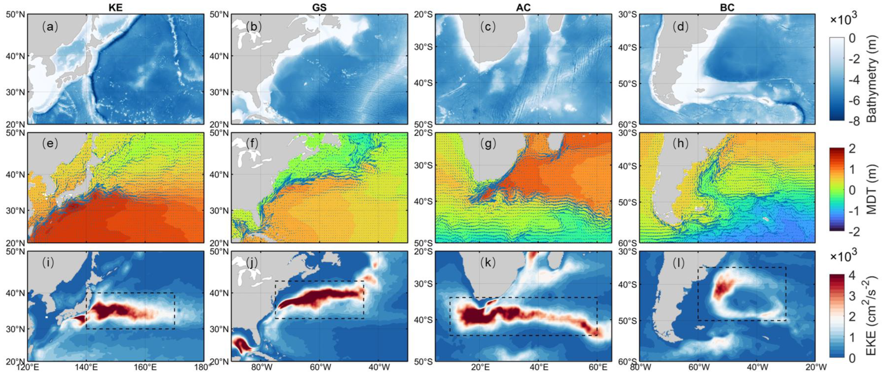
Mesoscale eddies are abundant and vigorous in the major western boundary current regions (WBCs) of the global ocean, i.e., the Kuroshio Extension (KE), the Gulf Stream (GS), the Agulhas Current (AC), and the Brazil Current (BC) [2,15,16,17]. Figure 1 gives the maps of bathymetry, mean dynamic topography, and eddy kinetic energy (EKE) in the four major WBCs. The four WBCs are all located in the western part of the wide oceans, and each has a strong pole-ward current along the western continental shelf. The Kuroshio and Gulf Stream are the two narrow and intense western boundary currents in the Northern Hemisphere. The main steams of the Kuroshio and Gulf Stream flow northward or northeastward along the continental shelf, and flow eastward as they break away from the shelf due to wind forcing, friction, and nonlinearity, forming strong eastward extension currents. Hence, the KE in this study is actually referred to as the Kuroshio after separation from the coast (Figure 1i). Studies have shown that the bends of the Kuroshio and Gulf Stream extension current often shed off many large cold and warm eddies which are visible in the satellite infrared images [18,19]. The western boundary current of the South Indian Ocean is the narrow, swift, westward Agulhas Current, which is one of the strongest currents in the global ocean, with maximum speeds that exceed 2.5 m/s [20,21]. Unlike the other three western boundary currents, the Agulhas Current overshoots the African coast (Agulhas leakage) and flows westward into the South Atlantic, and then part of it retroflects back at 20°E (Agulhas Retroflection) into the Indian Ocean and forms the eastward Agulhas Return Current. The large anticyclonic, warm, and saline eddies, known as the Agulhas rings, pinch off from the Agulhas Retroflection and play important roles in water exchange between the South Indian Ocean and the South Atlantic [22,23,24,25,26]. The Brazil Current is the western boundary current in the South Atlantic, which flows southward along the Brazil coast and meets the northward subantarctic Malvinas Current at about 38°S-40°S, forming the Brazil–Malvinas Confluence. The four WBCs are the regions with the highest eddy kinetic energy in the global ocean (Figure 1i–l); the energy is mainly from unstable currents and vigorous eddy activities [5,27]. Affected by strong eddy activities as well as strong current variabilities, the eddy–mean flow interaction is significant in the WBCs, through which the mean flow and eddies can exchange energy and momentum [28,29,30,31,32].
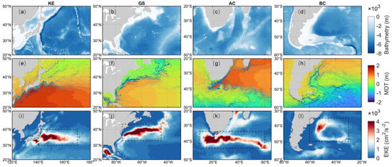
Figure 1.
The maps of bathymetry (a–d), geostrophic current and mean dynamic topography (MDT, e–h), and eddy kinetic energy (EKE, i–l) in the four WBCs (KE: Kuroshio Extension, GS: Gulf Stream, AC: Agulhas Current, BC: Brazil Current). The specific ranges of the four WBCs (KE: 30–40°N, 140–170°E; GS: 33–43°N, 45–75°W; AC: 34–44°S, 10–60°E; BC: 35–50°S, 30–60°W) are marked by dashed rectangles in (i–l).
Studies show that abundant and vigorous eddies have a significant impact on the heat and salt transport, air–sea interaction, and mixing in the WBCs [32,33,34,35]. Based on sixteen years of sea surface height fields, reference [2] provided a detailed investigation of mesoscale eddies in the global ocean and found that eddies in the WBCs have the largest amplitudes and are highly nonlinear (the ratio of the rotational speed to the movement speed). In most of the global ocean, eddies propagate westward with nearly the speed of the long baroclinic Rossby wave phase speed, while some eddies, limited in the WBCs, propagate eastward with the strong eastward background currents [36,37,38]. Based on satellite-derived sea surface height and temperature fields, the eddy identification in the KE and GS regions shows that the cyclonic-cold eddies predominantly exist on the south side of the mainstream, and anticyclonic-warm eddies are more likely distributed on the north side [39,40,41]. Reference [42] analyzed the statistical characteristics of mesoscale eddies in the North Pacific from satellite altimetry, and the results show that eddies have the largest amplitude and EKE in the KE region. Eddies in the KE region are generated through horizontal shear flow instability (barotropic instability) and meander development of the flow path [43,44,45]. Combining satellite data and Argo profiles, the three-dimensional eddy structure in the KE region was investigated, and a general westward strengthening and deepening of eddy anomalies were clearly observed [46,47,48]. Based on a high-resolution ocean model, reference [41] studied the eddy characteristics in the GS region and found that cyclonic eddies are smaller in size, but more energetic, and remain coherent longer than anticyclones. Recent analyses of eddies in the GS region reveal that cyclonic eddies contain cold water with elevated chlorophyll concentration and nutrients, while anticyclonic eddies contain warm water with reduced chlorophyll concentration and nutrients [49,50,51]. In the AC region, the Agulhas rings generally have long lifetimes and propagation distances (some of which can even reach the South American coast) and contribute a large part of Indian Ocean leakage into the Atlantic [26,52,53,54]. The census of AC eddies from satellite altimetry reveals that eddies with large radius and amplitude mainly occur in the Agulhas Retroflection [25,55,56]. In the BC region, the eddy identification and tracking show that most of the BC eddies do not propagate beyond the Argentine Basin and are advected by the Malvinas Current and the Zapiola Drift [55,57]. Reference [58] suggested that Zapiola Drift sheds anticyclonic eddies to its outer portion and cyclonic eddies to its inner portion.
At present, the studies of oceanic mesoscale eddies usually use some statistics of eddy kinetic properties in the global ocean based on altimetry sea surface height data, or some local studies of eddy vertical structures and thermohaline properties in a certain region based on multisource data. Studies on mesoscale eddies in the four major WBCs of the global ocean have not been systematically carried out. There is a lack of comparative analysis of eddy properties in the four WBCs, especially the different effects of eddy activities on local sea surface temperature, salinity, density, chlorophyll concentration, and vertical thermohaline structure in different WBCs. Mesoscale eddies can cause the sea surface to rise or fall due to the geostrophic motion, which can generally be identified as enclosed regions in the sea surface height anomaly (SSHA) field. In this study, based on long time series of satellite altimeter SSHA data, the eddy identification and tracking are carried out in the four WBCs, and the eddy properties (e.g., eddy trajectory, lifetime, propagation distance, amplitude, radius) are systematically analyzed. Mesoscale eddies can also change the temperature, salinity, density, and chlorophyll concentration of the surface water due to the vertical movement of water bodies in the eddy. The multisource satellites provide the daily sea surface temperature (SST), sea surface salinity (SSS), sea surface density (SSD), and chlorophyll concentration (CHL) products. Therefore, combining the altimeter-detected eddy results with the simultaneous observations of SST, SSS, SSD, and CHL, the local impacts of eddy activities in each WBC are analyzed. In addition, the ocean subsurface temperature and salinity information can be provided by Argo profiles. Through the temporal–spatial matching of eddy results and Argo profiles, the analysis on the vertical thermohaline characteristics of mesoscale eddies in the four WBCs is carried out. This work helps us to increase our knowledge of mesoscale eddy properties in four major WBCs of the global ocean and to understand the regional effects of eddy activities on surface temperature, salinity, density, and chlorophyll concentration, as well as the subsurface thermohaline structure. The comparative analysis of eddy properties is important for further research on the eddy-induced volume transport, the regional balance of heat and salinity, and the local air–sea interaction in the WBCs.
The rest of the paper is organized as follows. Section 2 describes the materials and methods. Section 3 presents the results of eddy properties in the four WBCs based on satellite altimeter SSHA data. Section 4 discusses the surface temperature, salinity, density, and chlorophyll concentration characteristics, as well as the vertical thermohaline characteristics of mesoscale eddies in the four WBCs. Finally, the summary and conclusions are given in Section 5.
2. Materials and Methods
2.1. Data
2.1.1. The Multi-Altimeter Merged SSHA Product
Mesoscale eddies are generally identified as enclosed regions in the satellite altimeter SSHA field. The sea surface height anomaly (SSHA) data used in this study are the multi-altimeter merged sea level product (SEALEVEL_GLO_PHY_L4_MY_008_047, https://doi.org/10.48670/moi-00148, accessed on 12 June 2023), which is daily, global coverage, with a spatial resolution of 1/4°. This product is processed by the Ssalto/Duacs multimission altimeter data processing system and distributed by the European Copernicus Marine Environment Monitoring Service (CMEMS) [59]. In this study, a 30-year period of the SSHA product from January 1993 to December 2022 is used to determine the presence and positions of mesoscale eddies in the four WBCs.
2.1.2. The NOAA OISST Product
The satellite SST maps can capture the surface temperature changes caused by mesoscale eddies. The NOAA provides the daily Optimum Interpolation SST (OISST) product Version 2.1 (https://doi.org/10.25921/RE9P-PT57, accessed on 15 November 2023) on a regular grid of 1/4°, which is constructed by using satellite SST maps from the Advanced Very High-Resolution Radiometer (AVHRR) [60,61]. This study used 30 years of the OISST product, from January 1993 through December 2022. In order to identify mesoscale variabilities, the daily SST anomalies (SSTAs) are calculated by subtracting the seasonal-mean climatologic fields computed by averaging all SST fields in the season. The SST climatologic season (including the latter SSS, SSD, and CHL) are consistent with the World Ocean Atlas 2023, as Jan.–Mar., Apr.–Jun., Jul.–Sep., and Oct.–Dec.
2.1.3. The Sea Surface Salinity and Density Product
The multi-observation global ocean sea surface salinity (SSS) and sea surface density (SSD) product (MULTIOBS_GLO_PHY_S_SURFACE_MYNRT_015_013, https://doi.org/10.48670/moi-00051, accessed on 6 August 2023) consists of daily global gap-free analyses of the SSS and SSD at 1/8° of spatial resolution, developed by the Consiglio Nazionale delle Ricerche and distributed by CMEMS [62]. In this study, a 30-year period of the product from January 1993 to December 2022 is used to determine the SSS and SSD signals of mesoscale eddies. Similarly to the SSTAs, the daily SSS anomalies (SSSAs) and SSD anomalies (SSDAs) are calculated by subtracting the seasonal-mean climatologic fields computed by averaging all SSS and SSD fields in the season.
2.1.4. The Global Ocean Color Product
The global ocean color product (OCEANCOLOUR_GLO_BGC_L4_MY_009_104, https://doi.org/10.48670/moi-00281, accessed on 15 November 2023) from multi-sensor observations provides the daily global chlorophyll-a (CHL) concentration in sea water, with a spatial resolution of 4 km. The merging CHL product is processed the Copernicus-GlobColour project and distributed by CMEMS [63]. In this study, a 25-year period of the product from January 1998 to December 2022 is used to determine the CHL variances of mesoscale eddies. Similarly to the SSTAs, the CHL anomalies (CHLAs) are calculated by subtracting the seasonal-mean climatologic fields computed by averaging all CHL fields in the season.
2.1.5. Argo Profiles Data
The effect of eddies on the vertical temperature and salinity are studied using available Argo profiles in the global ocean, provided by the Coriolis Global Data Acquisition Center of France (https://data-argo.ifremer.fr, accessed on 20 October 2023). In the analysis, we have taken pressure, temperature, and salinity profiles with quality flag 1 from January 1998 to December 2022. Furthermore, following references [64,65], all profiles were selected under the conditions: (1) the shallowest data are located between the surface (0 dbar) and 10 dbar pressure, and the deepest data are below 1000 dbar; (2) the pressure difference between two consecutive records does not exceed a given limit (25 dbar for the 0–100 dbar layer, 50 dbar for the 100–300 dbar layer, 100 dbar for the 300–1000 dbar layer); (3) each profile should contain at least 30 valid records in the upper 1000 dbar; (4) any suspicious profiles with evident errors (e.g., the Pauta criterion) in temperature or salinity records are discarded. The final dataset includes a total more than two million (2,196,009) available profiles in the global ocean. Potential temperature θ and salinity S data in each profile were linearly interpolated onto the vertical normal levels from the surface (0 dbar) to 2000 dbar (or to the deepest layer of the profile, if the profile did not exceed 2000 dbar) with an interval of 20 dbar, using the Akima spline method. To get the thermohaline structures of mesoscale eddies, the potential temperature anomaly θ′ and salinity anomaly S′ of the Argo profiles were computed by removing seasonal-mean climatologic fields on a 1° grid for the three decades of 1991–2020 from the World Ocean Atlas 2023 [66].
2.2. Eddy Identification and Tracking
Mesoscale eddies can cause the sea surface to rise or fall due to geostrophic motion, which can generally be identified as enclosed regions in the SSHA field. Based on the daily SSHA field from January 1993 to December 2022, mesoscale eddies are identified through Chelton’s geometric algorithm of SSHA-enclosed contours in the four WBCs [2]. For the SSHA field with a 1/4° spatial grid, identified eddies should include at least 8 grid cells and fewer than 1000 grid cells to avoid too-small or too-large vortex-like features. Based on the eddy identification results in the continuous time series, the evolution process of eddies (eddy trajectories) in the ocean can be tracked by comparing the eddy positions and dynamic properties [67,68]. As long as an eddy appears or disappears within the four WBCs, its complete eddy trajectory is tracked and preserved. In the study, only eddies with a lifetime ≥ 30 days (1 month) are analyzed to ensure that the eddy results identified from the SSHA field are coherent mesoscale dynamic process, rather than transient turbulence signals.
2.3. Eddy Surface and Vertical Signals
Mesoscale eddies are a kind of typical geostrophic dynamic process which can cause vertical movement of water bodies, thereby changing the temperature, salinity, density, and chlorophyll concentration of the surface water in the eddy. Based on a 30-year period of SSHA-identified mesoscale eddies with a lifetime ≥ 1 month, eddy surface signals are analyzed through temporal–spatial matching of eddies with daily SSTA, SSSA, SSDA, and CHLA data. Surface remote sensing data on the same day as the eddy results and located within the range of two times the eddy radius are selected for the study of eddy surface signals. The remote sensing data in the eddy are transformed into a normalized and non-dimensional eddy-coordinate system by calculating the relative position of the remote sensing data to the eddy core [50,69]. The averaged SSTA, SSSA, SSDA, and CHLA signals of the normalized eddies in each WBC region are calculated based on all the matched results of eddies and the surface data on long time series.
The surface signals of mesoscale eddies are easily observed by multi-source remote sensing. Moreover, mesoscale eddies can cause the vertical temperature and salinity changes of the water masses due to upwelling and downwelling, which can be captured by in situ Argo float profiles. The eddy vertical signal is constructed by surfacing the Argo float profiles into SSHA-identified eddy areas [64,65]. The Argo profiles on the same day as the eddy results and located within the eddies are selected for eddy vertical signal analysis. Through temporal–spatial matching of the SSHA-identified eddies and Argo profiles over a long time (from the year 1998 to 2022), a large number of Argo profiles within eddies can be obtained. The thermohaline structure of eddies in each WBC region can be obtained by averaging all vertical temperature and salinity signals based on all Argo profiles within regional eddies [40,46].
3. Results
3.1. Eddy Trajectory, Lifetime, and Propagation Distance
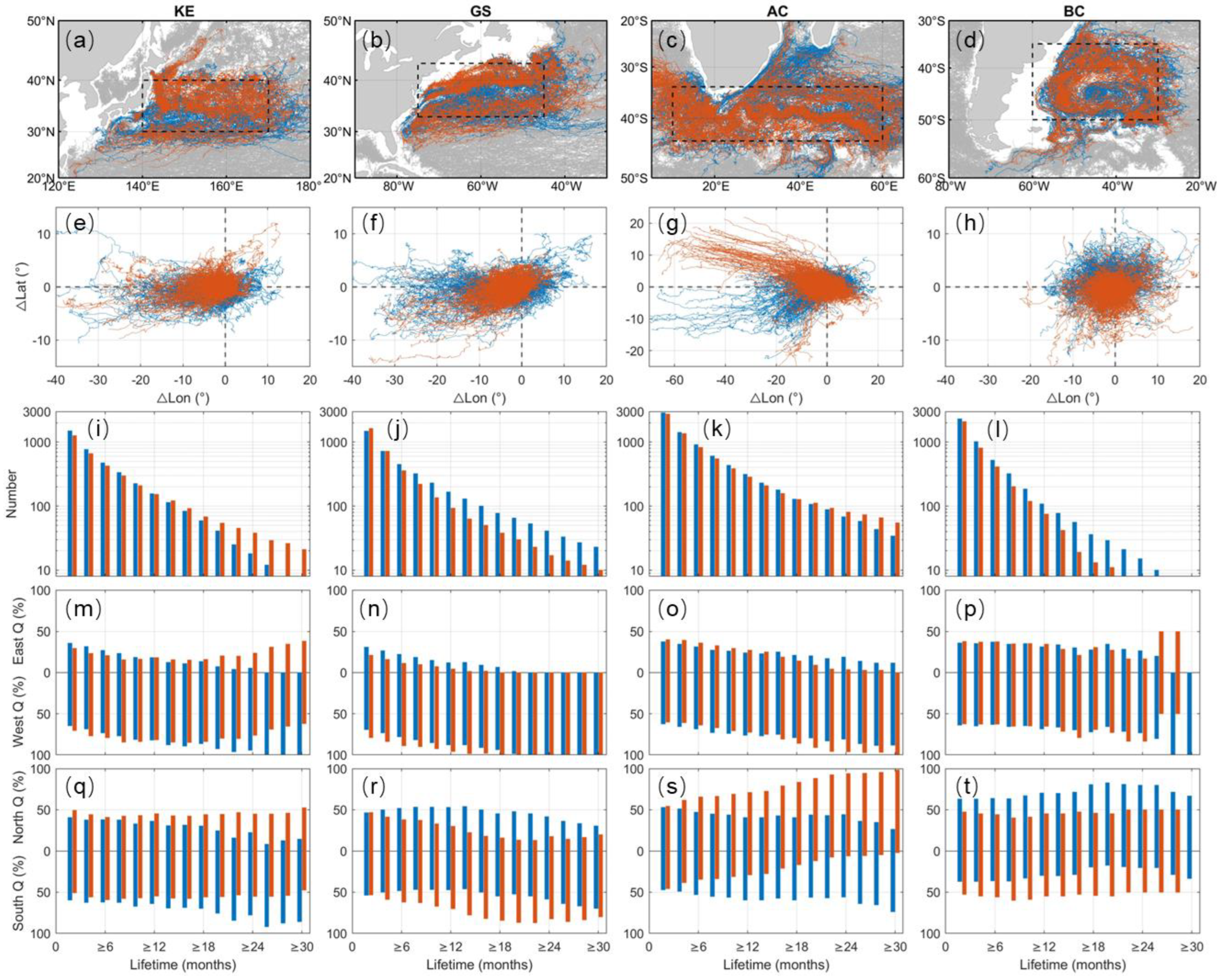
Based on 30 years of satellite altimeter SSHA data from January 1993 to December 2022, the identification and tracking of mesoscale eddies in the four WBCs are carried out, and the results of mesoscale eddies with a lifetime ≥ 1 month are obtained. In order to reveal the geographical distribution of mesoscale eddies in the four WBCs, eddy trajectories with a lifetime ≥ 6 months are displayed in Figure 2a–d (not all eddy trajectories are displayed to avoid a chaotic and unreadable map). It can be seen that both cyclonic eddies and anticyclonic eddies are abundant in the four WBCs, and many eddies that appear in the WBCs can still move farther away when they move outside the WBCs. To observe the propagation directions of mesoscale eddies, the apparent positions of eddy trajectories are moved to the origin position, and the relative propagation trajectories of eddies are obtained (Figure 2e–h). Eddies with long distances in the KE, GS, and AC regions show an obvious westward propagation trend. In contrast, fewer eddies in the BC region have long propagation trajectories. Eddies in the BC region are largely confined to the Brazil–Malvinas confluence due to the restriction of the South American continent to the west and the influence of the eastward Antarctic Circumpolar Current to the south [55,56]. In the four WBCs, there are a certain number of eddies with eastward propagation trajectories, which are advected by the strong eastward extension currents [2,36]. Compared to the westward eddies, the eastward eddies do not propagate far due to the high sensitivity to changes in flow and wind speed [37,70]. It is worth noting that in the KE region, some anticyclonic eddies that formed along the Japan Trench or split off from the western meander of the Kuroshio can move a long distance northward and eastward along the Kuril Trench [71], this feature being remarkably different from the other WBCs.
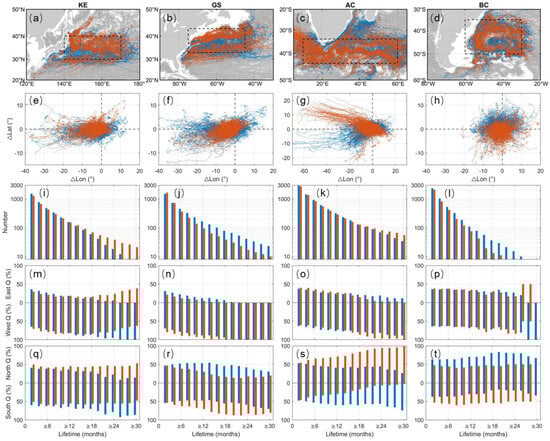
Figure 2.
The map of eddy trajectories (a–d) and relative propagation trajectories (e–h) with a lifetime ≥ 6 months; the numbers (i–l), the west- and eastward proportions Q (m–p), and the south- and northward proportions Q (q–t) of eddy trajectories exceeding a certain lifetime (e.g., 2, 4, 6 months, etc.) in the four WBCs. The blue lines or bars represent cyclonic eddies, the red lines or bars represent anticyclonic eddies, and the dashed lines in a-d are the specific ranges of the four WBC; the gray lines in a-d represent eddy trajectories that do not enter the WBCs.
The numbers of mesoscale eddies exceeding a certain lifetime (e.g., 2, 4, 6 months, etc.) in the four WBCs are given in Figure 2i–l. The eddy number decreases rapidly with the increase in lifetime, indicating that most eddies still exhibit short lifetimes in the WBCs. Compared with the other three WBCs, the AC region has the highest number of long-lived eddies (e.g., lifetime exceeding 1 year). This is because the AC is not blocked by continents on the western side, and mesoscale eddies (especially, the Agulhas rings) generated in the region can propagate westward across the southern coast of Africa into the broad South Atlantic Ocean, and then continue to propagate westward for a long distance (Figure 2c,g). In terms of eddy polarity, long-lived eddies in the KE region are predominantly anticyclonic eddies, while long-lived eddies in the GS and BC region are predominantly cyclonic eddies, and the polarity difference is not obvious in the AC region. The analysis of long-lived eddy trajectories shows that the KE region has many anticyclonic eddies with long lifetimes on the north side of the KE, especially for the Tohoku anticyclonic eddies, which slowly drift northeastward along the Japan–Kuril Trench (Figure 2a) [71,72]. In the GS region, there are fewer long-lived anticyclonic eddies on the north side of the mainstream, while cyclonic eddies on the south side of the current have a broad space to propagate in the ocean, and their lifetimes and propagation distances are longer.
In order to further analyze the propagation direction of eddies in the four WBCs, the westward and eastward proportions (Figure 2m–p) and the southward and northward proportions (Figure 2q–t) of eddy trajectories exceeding a certain lifetime (e.g., 2, 4, 6 months, etc.) are calculated. It can be seen that eddies in the WBCs mainly propagate westward, especially with the increase in lifetime, and that the proportions of westward eddies are higher (except for the anticyclonic eddies in the KE region). This indicates that westward eddies generally have longer lifetimes, while eastward eddies tend to have short lifetimes and propagation distances. In terms of the south- and northward proportions (Figure 2q–t), eddies in different regions show different propagation tendencies. In the KE region (Figure 2q), the southward proportion of the cyclonic eddies increases with the increase in lifetime, whereas the anticyclonic eddies have little difference in the south- and northward proportions. The long-lived anticyclonic eddies in the GS region (Figure 2r) show a southward tendency. In the AC region (Figure 2s), the cyclonic and anticyclonic eddies show obvious southward and northward tendencies, respectively, which become more pronounced with the increase in lifetime. The different propagation directions of different types of mesoscale eddies are critical for the transport of water masses carried within the eddies [38,73,74].
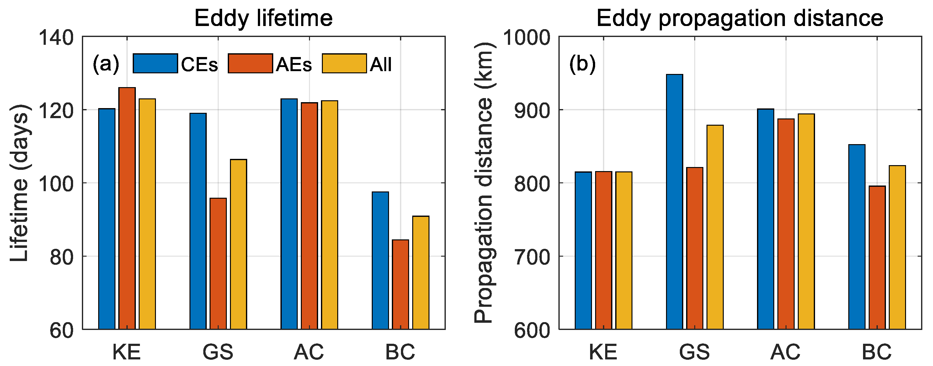
The mean lifetime and propagation distance of all eddies with a lifetime ≥ 1 month in the four WBCs are given in Figure 3. Eddies in the KE and AC regions have longer lifetimes; the mean lifetimes of both regions exceed 120 days (4 months). Eddies in the GS region have a mean lifetime of 106 days (about 3.5 months), and eddies in the BC region have the shortest mean lifetime of only 91 days (about 3 months). The mean propagation distance of eddies in the AC region is the largest, nearly 900 km, which is mainly due to the fact that some long-lived eddies can propagate westward for a long distance (Figure 2c,g). Among the four WBCs, eddies in the KE region have the smallest propagation distance but a long lifetime, which indicates that KE eddies propagate relatively more slowly. In terms of eddy polarity, in the GS and BC regions, the mean lifetime and propagation distance of cyclonic eddies are larger than those of anticyclonic eddies. The polarity difference of eddies in the KE and AC regions is small.
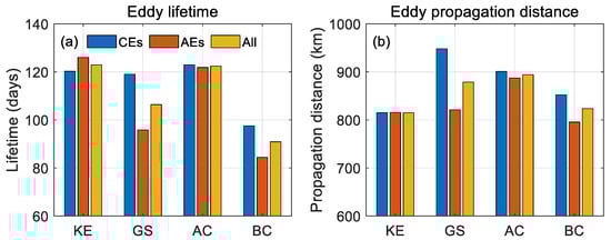
Figure 3.
The mean lifetime (a) and propagation distance (b) of all SSHA-identified eddies (CEs are cyclonic eddies; AEs are anticyclonic eddies; All includes all eddies) with a lifetime ≥ 1 month in the four WBCs.
3.2. Geographical Distributions of Eddy Number, Polarity, Amplitude, and Radius
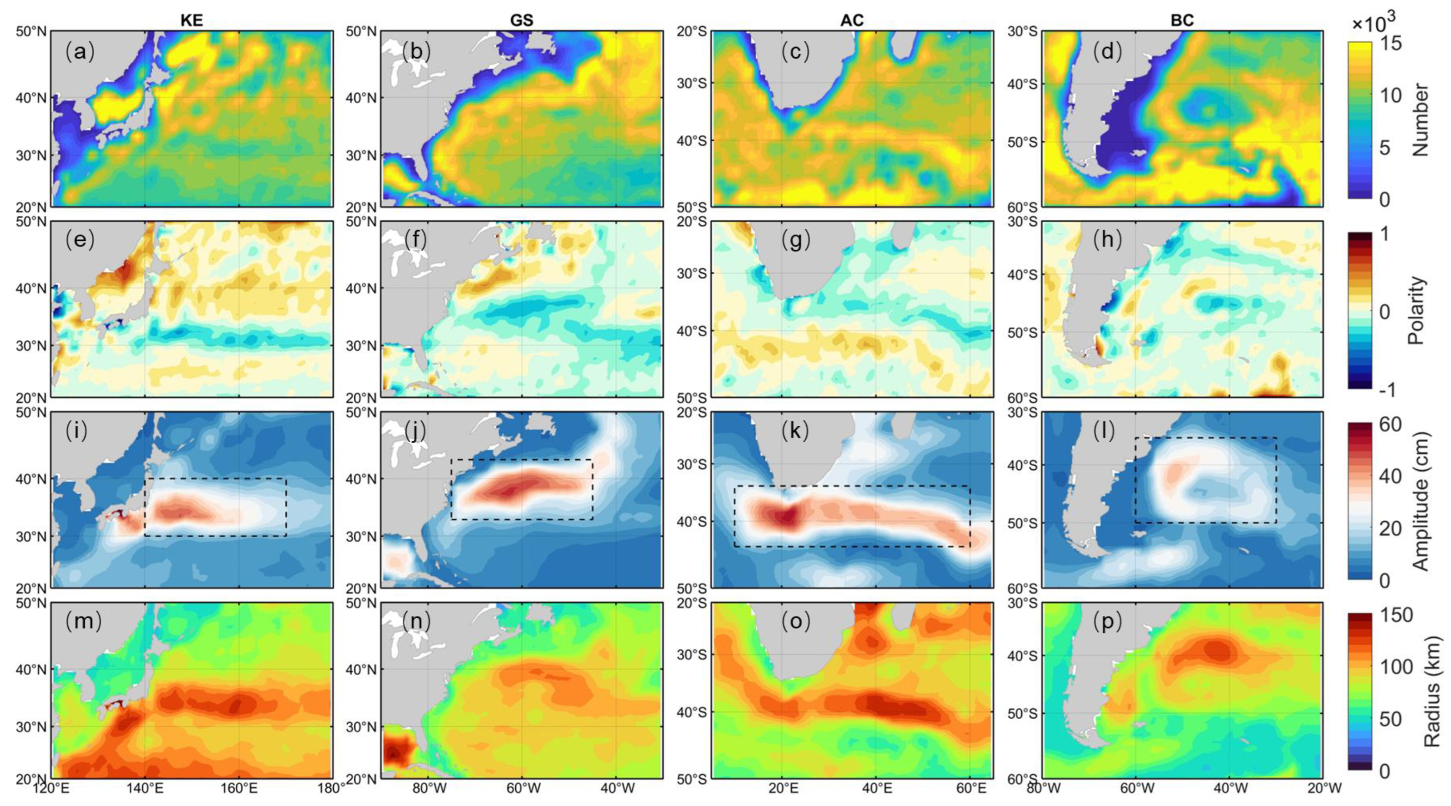
In order to reveal the geographical distribution of eddy properties in the four WBCs, the eddy number, polarity, amplitude, and radius in grid windows of 1° × 1° are counted based on 30 years of SSHA-identified eddies. The eddy polarity in a grid indicates that eddies in the grid tend to be cyclonic (when the value is negative) or anticyclonic (when the value is positive) [67]; it is calculated as Polarity = (NAE – NCE)/(NAE + NCE), where NAE and NCE are the numbers of anticyclonic and cyclonic eddies in one region, respectively. The eddy amplitude is the difference between the minimum and maximum values of the SSHA in the eddy area, which generally represents eddy strength. The eddy radius is defined as the equivalent radius of a circle with the same area as the eddy. The maps of eddy number, polarity, amplitude, and radius in the four WBCs are given in Figure 4.
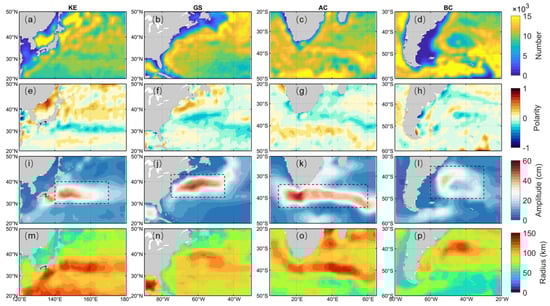
Figure 4.
The maps of eddy number (a–d), polarity (e–h), amplitude (i–l), and radius (m–p) from SSHA-identified eddies with a lifetime ≥ 1 month in the four WBCs. The specific ranges of the four WBCs are marked by dashed lines in (i–l).
The geographical distributions of eddy number (Figure 4a–d) shows that eddies are clustered along the mainstream axis in the four WBCs. In particular, the high occurrence of eddies in the BC region forms a ring shape along the Brazil–Malvinas confluence, inside which the eddy number is low. The maps of eddy polarity (Figure 4e–h) shows that there are different types of eddy tendencies to the north and south sides of the WBC mainstream. Specifically, for the KE and GS in the Northern Hemisphere, eddies on the north side of the mainstream tend to be anticyclonic, and eddies on the south side tend to be cyclonic. The eddy preference is due to the fact that the eastward mainstream bends to the north and spins off clockwise vortices with anticyclonic vorticity on the north side (generally carrying warm water), and the eastward mainstream bends to the south and spins off counterclockwise vortices with cyclonic vorticity on the south side (generally carrying cold water) [39,40,41]. In contrast to the KE and GS, the AC and BC in the Southern Hemisphere tend to have cyclonic eddies (cold eddies) on the north side and anticyclonic eddies (warm eddies) on the south side of the mainstream. On the whole, eddies in the WBCs have an anticyclonic preference on the polar-ward side and a cyclonic preference on the equator-ward side.
From the maps of eddy amplitude (Figure 4i–l), it can be seen that eddy amplitudes are significantly higher in the four WBCs than in the other oceans. The Agulhas Retroflection (Figure 4k), where the AC reverses to form the return current, has the highest eddy amplitude in the global ocean, with an average amplitude of more than 50 cm. The AC is the fastest ocean current, and once it reverses, it pinches off fast-rotating eddies (which can also be seen from the EKE map in Figure 1k), which can cause large sea surface height fluctuations. Therefore, strong eddies with large amplitudes can be often observed here [25,30,55]. In contrast, the eddy amplitude in the BC region is relatively low. The southward Brazil Current is not as strong as the other three WBCs [33] (also as shown in Figure 1h,l), and it encounters the northward Malvinas Current along the western margin of the Argentine Basin and forms the Brazil–Malvinas Confluence, where the current velocity is weakened. As a result, eddies generated in the BC region have relatively low strength, caused by sea surface height fluctuations, not as large as in the other three WBCs. The geographical distributions of eddy radius in the four WBCs are shown in Figure 4m–p. Similarly to the maps of eddy amplitude, the eddy radii are significantly larger in these WBCs than in the other oceans (especially compared to the same latitude regions). Among the four WBCs, eddies in the Kuroshio extension region and the Agulhas return current region have the largest radius, which can reach an average radius of 150 km.
In order to quantitatively compare eddy properties in the four WBCs, the regionally averaged amplitude and radius of mesoscale eddies are calculated and given in Figure 5. It can be seen that the average amplitude of eddies in the GS region is the largest (about 21 cm), while that in the BC region is the smallest (about 15 cm). The average amplitudes of eddies in the KE and AC regions are about 17 cm and 18 cm, respectively. An interesting point is that the average amplitude of the cyclonic eddies is higher than that of the anticyclonic eddies in all four WBCs, especially for the GS region. In terms of eddy radius, the average radii of eddies in the four WBCs are not much different. Eddy radius is slightly larger in the KE region and slightly smaller in the BC region, and the polarity difference of eddy radius is not significant.
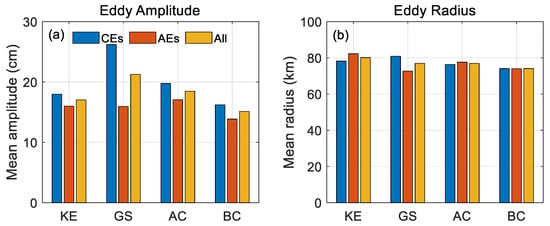
Figure 5.
The regionally averaged amplitude (a) and radius (b) of all SSHA-identified eddies (CEs are cyclonic eddies; AEs are anticyclonic eddies; All includes all eddies) with a lifetime ≥ 1 month in the four WBCs.
4. Discussion
4.1. Characteristics of Surface Temperature, Salinity, Density, and Chlorophyll Concentration of Mesoscale Eddies
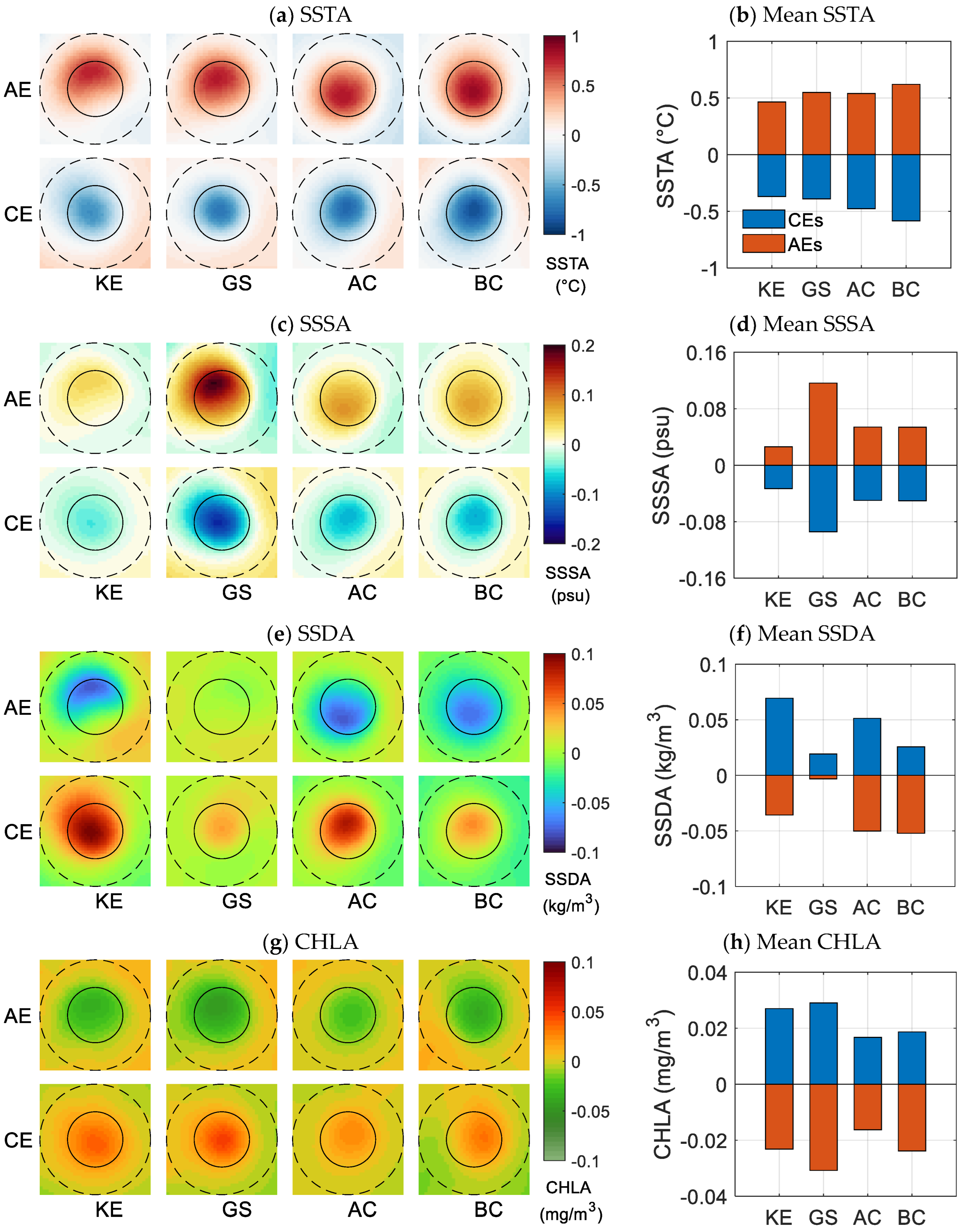
The most obvious feature of mesoscale eddies on the sea surface is that they can cause sea surface height fluctuations, so it is easy to observe and identify them from the satellite SSHA field. At present, most of mesoscale eddy research in the ocean is based on the satellite altimetry data. A mesoscale eddy is a kind of typical geostrophic dynamic process which can cause vertical movement of water bodies, thereby changing the temperature, salinity, density, and chlorophyll concentration of the surface water in the eddy [9,51,69]. Based on a 30-year period of SSHA-identified mesoscale eddies with a lifetime ≥ 1 month, eddy surface signals are analyzed through temporal–spatial matching of eddies with the simultaneous observations of SSTA, SSSA, SSDA, and CHLA data. The average statistical results of eddy SSTA, SSSA, SSDA, and CHLA signals over 30 years are shown in Figure 6 (there were only 25 years of CHLA data).
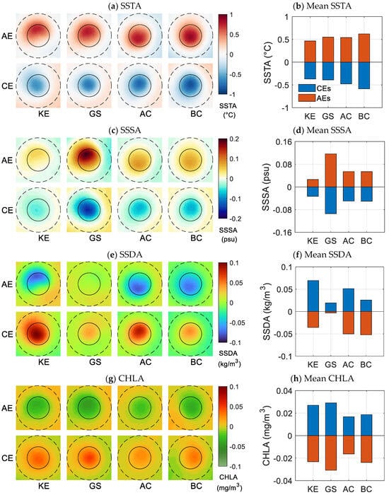
Figure 6.
The SSTA (a), SSSA (c), SSDA (e), and CHLA (g) signals of the normalized eddy (CE is the cyclonic eddy; AE is anticyclonic eddy; the solid lines represent the normalized eddy area; the dotted lines represent the range of two times the eddy radius), and the averaged SSTA (b), SSSA (d), SSDA (f), and CHLA (h) values within the normalized eddy area (solid line) in the WBCs based on a 30-year period of SSHA-identified eddies and multi-source remote sensing data.
For the eddy-induced SST changes (Figure 6a), the SSTA signals within eddies are basically the same in the four WBCs, with positive SSTAs (warm eddies) in the anticyclonic eddies and negative SSTAs (cold eddies) in the cyclonic eddies, and the SSTA signals outside eddies are weak. Although some studies have found that there are some “abnormal” eddies (e.g., cyclonic warm eddies or anticyclonic cold eddies) in the ocean [75,76], the average statistical results on long time series show that the climatological state of SSTA signals in eddies is normal in the four WBCs, i.e., cyclonic cold eddies and anticyclonic warm eddies. In terms of the magnitude of eddy-induced SSTA signals (Figure 6b), the BC region has the largest value for both anticyclonic and cyclonic eddies (exceeding 0.6 °C), while the KE region has the smallest value. Similarly to eddy SSTA signals, the mean SSSA signals within eddies (Figure 6c,d) are positive for anticyclonic eddies and negative for cyclonic eddies in all four WBCs, but the magnitude of SSSAs varies greatly in different regions. Compared with the other three WBCs, eddies in the GS region have the largest magnitude of SSSA signals, with a mean SSSA of about 0.11 psu for anticyclones and closing to −0.1 psu for cyclones. This is partly due to the large vertical salinity gradient in the GS region, where the vertical movement of eddies causes large changes in sea surface salinity. On the other hand, the meridional gradient of surface salinity in the GS region is also larger than that of the other three WBCs [19]; the meridional movement of eddies causes a larger salinity difference between the surface waters within eddies and the surrounding waters. The mean SSSA magnitude of eddies in the KE region is the smallest (due to both the small vertical salinity gradient and the small meridional gradient of surface salinity), less than 0.03 psu, and the values in the AC and BC regions are around 0.05 psu.
For the eddy-induced sea surface density changes (Figure 6e,f), the mean SSDA signals within eddies are negative for anticyclonic eddies and positive for cyclonic eddies, which are opposite to those of eddy SSTA and SSSA signals. The magnitude of mean SSDA signals within eddies in the KE region is the largest, and the value in the GS region is the smallest. The weak SSDA signals of eddies in the GS region are mainly due to the large SSSA neutralizing the density changes in surface waters caused by temperature changes. For example, in the GS region, a positive (negative) SSTA within the anticyclonic (cyclonic) eddies causes a decrease (increase) in the density, but the corresponding high positive (negative) SSSA can cause an increase (decrease) in the density. As a result, the two effects neutralize each other, making the density changes of surface water within eddies insignificant. The weak SSSA signals of eddies has little influence on the surface density changes, so the SSDAs of eddies mainly caused by SSTAs are large in the KE region. The surface density changes of eddies in the AC and BC regions are similar to those of the KE region. Consistent with SSDA signals, the mean CHLA signals within eddies (Figure 6g,h) are negative for anticyclones and positive for cyclones in all four WBCs. In general, the upwelling caused by cyclonic eddies brings nutrients from under the ocean to the surface, which can contribute to phytoplankton growth and increase CHL concentrations (i.e., positive CHLA) [9,13,51]. In contrast, anticyclonic eddies have fewer nutrients on the surface due to the convergence of the water, which can hinder phytoplankton growth and reduce the CHL concentrations (i.e., positive CHLA). Regionally, the magnitudes of eddy CHLA signals are larger in the KE and GS regions and smaller in the AC and BC regions.
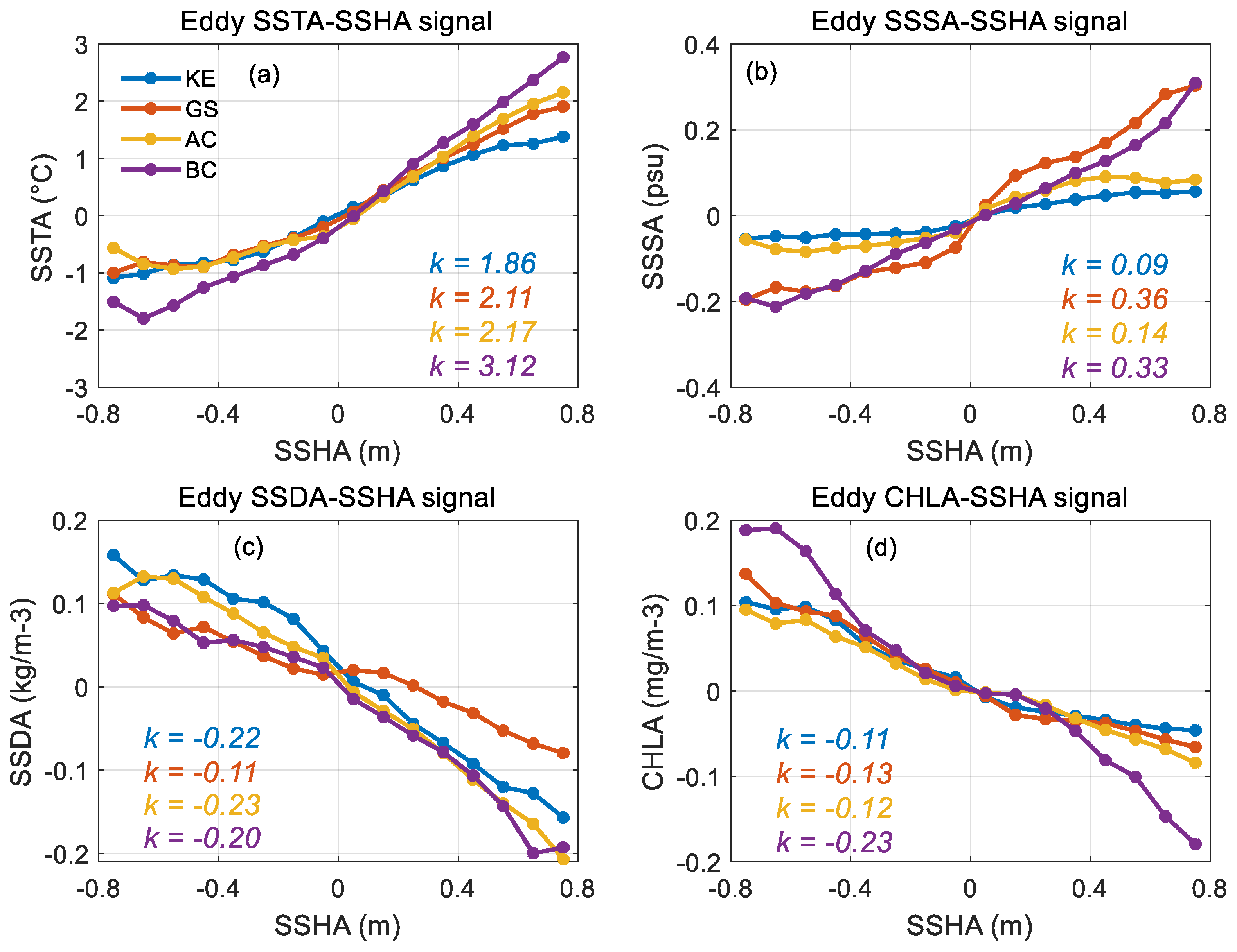
Compared with the eddy amplitude for the four WBCs in Figure 5a, the SSTA, SSSA, SSDA, and CHLA signals in mesoscale eddies show more regional differences. In order to study the relationship between the changes in eddy surface signals and the SSH changes in eddies in the different regions, the correlations between eddy SSTA, SSSA, SSDA, and CHLA signals with eddy SSHA signal are analyzed. In this analysis, the averages of the surface signals in the eddy area with the same SSHA signals are calculated in the four WBCs, and the results are shown in Figure 7. In addition, the linear regression coefficients k(surface signals/SSHA) are also given in the figure. Overall, in all four WBCs, the eddy SSTA and SSSA signals are positively correlated with the eddy SSHA signal, while the eddy SSDA and CHLA signals are negatively correlated with the eddy SSHA signal. The correlations of eddy SSTA–SSHA signals (Figure 7a) show that the coefficient k(SSTA/SSHA) is largest in the BC region and smallest in the KE region. This suggests that mesoscale eddies with the same intensity can cause a large SST change in the BC region, but less change in the KE region. This also explains that eddies in the BC region have the largest SSTA signal, although their mean eddy amplitude is the smallest among the four WBCs. The correlations of eddy SSSA–SSHA signals (Figure 7b) show that the coefficient k(SSTA/SSHA) is large in the GS and BC regions, and small in the KE and AC regions. The correlations of eddy SSDA–SSHA signals (Figure 7c) show that the coefficient k(SSDA/SSHA) is small in the GS region, which suggests that the eddy-induced density change is weak (Figure 6f). The correlations of eddy CHLA–SSHA signals (Figure 7d) show that the eddy CHLA signal does not differ much in the four WBCs for low SSHA eddies, but the CHLA is significantly larger in the BC region when the eddy SSHA exceeds ±0.4 m.
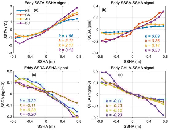
Figure 7.
The average of SSTA (a), SSSA (b), SSDA (c), and CHLA (d) signals of eddies for the different SSHA signals in the four WBCs; the regression coefficients k(SSTA/SSHA), k(SSSA/SSHA), k(SSDA/SSHA), and k(CHLA/SSHA) are labeled in the figure.
4.2. Vertical Thermohaline Characteristics of Mesoscale Eddies in the Four WBCs
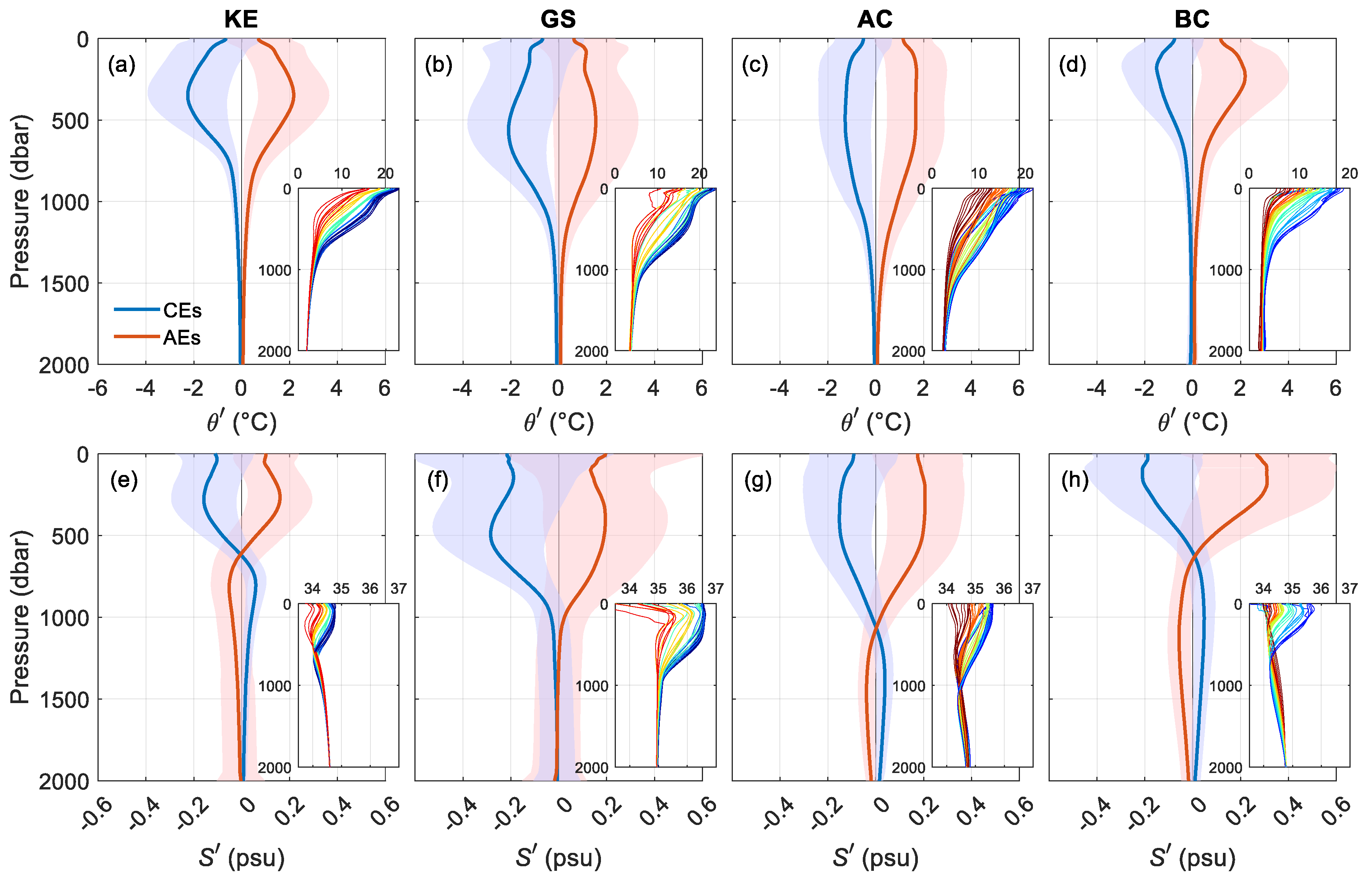
Combining the SSHA-identified eddies with Argo profile data over a 25-year period from 1998 to 2022, the vertical thermohaline characteristics of mesoscale eddies in the four WBCs were analyzed by three-dimensional eddy reconstruction. Mean vertical profiles of temperature anomaly θ′ and salinity anomaly S′ inside eddies in the four WBCs are shown in Figure 8. The vertical θ′ profiles (Figure 8a–d) show that mean θ′ caused by eddies is negative for cyclonic eddies and positive for anticyclonic eddies in all four WBCs. The vertical temperature changes in eddies are not only related to the vertical downwelling of waters in eddies, but also relate to the eddy movement (e.g., for the KE and GS regions, cyclonic eddies carry subpolar cold water equator-ward and anticyclonic eddies carry subtropical warm water pole-ward). The maximum eddy θ′ values in the KE and GS regions are ±2 °C, with the corresponding depths at 400 dbar and 600 dbar, respectively, which are consistent with the previous researches [46,48,77]. The maximum eddy θ′ values in the AC and BC regions are about ±1.5 °C, with the corresponding depths at 500 dbar and 200 dbar. In comparison, the vertical temperature changes caused by eddies in the KE and BC regions are shallow, largely concentrated at depths shallower than 600 dbar (corresponding to the depth of the main thermocline, as shown in the lower-right subfigure in Figure 8a). In particular, in the BC region, the eddy influence on underwater temperature is largely concentrated in the subsurface ocean, with the largest θ′ close to sea surface, which may also explain why eddies in the BC region have the lowest eddy amplitude, but the largest SSTA signal (Figure 6a,b). In the GS and AC regions, mesoscale eddies have a deep vertical temperature influence, exceeding 1000 dbar. Especially in the AC region, although the maximum eddy θ′ is lower than that in the KE and GS regions, eddies have large and similar-size θ′ at the depths of 200–1000 dbar, and the influence of depth on vertical temperature is the deepest among the four WBCs.
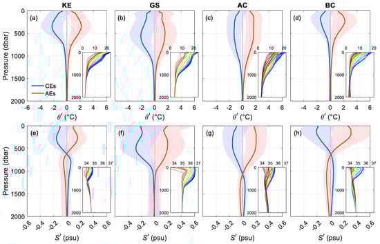
Figure 8.
Mean vertical profiles of temperature anomaly θ′ (a–d) and salinity anomaly S′ (e–h) inside eddies (CEs are cyclonic eddies; AEs are anticyclonic eddies) in the four WBCs; the shading indicates one standard deviation value range. The climatological temperature and salinity profiles of water masses based on WOA 2023 in a 5°lon × 2°lat subregion for the four WBCs are also given in the lower-right corner of the figure (colors represent different latitudes, blue represents the low latitude, and red represents the high latitude; absolute values are taken for the latitudes of AC and BC in the Southern Hemisphere).
Compared with vertical temperature changes, the vertical salinity changes inside eddies (Figure 8e–h) are more variable. In the upper layers of the ocean in the four WBCs, cyclonic eddies have negative S′ (upwelling of low-saline water) and anticyclonic eddies have positive S′ (sinking of high-saline surface water). However, in the shallow water layers (shallower than 100 dbar), some regions are covered with low-saline surface water, so that eddy S′ has a large fluctuation range, even opposite sign near the sea surface (e.g., a large standard deviation in the GS region, as shown in Figure 8f). In comparison, eddies have the maximum S′ exceeding ±0.2 psu at the depths of about 500 dbar in the GS region and near the surface in the BC region. In the KE and AC regions, the maximum values of eddy S′ are located at the depths of about 300 dbar and 400 dbar, respectively. In the GS region, the mean vertical profiles of eddy S′ have a single sign from the surface to the deep ocean. In contrast, below a certain depth in the other three WBCs (about 600 dbar for the KE and BC region, and 1000 dbar for the AC region), the signs of eddy S′ are reversed, with positive values in cyclones and negative values in anticyclones. The reversed signs of eddy S′ in the lower layers are also reported by references [44,57]. This is closely related to the salinity changes in water masses with depth in these regions: salinity decreases with increasing depth above a certain depth, and salinity increases with increasing depth below a certain depth (the lower-right subfigure in Figure 8e,g,h). Therefore, the upwelling or downwelling caused by eddies can lead to different S′ signals above or below the depth in the KE, AC, and BC regions. Moreover, the magnitudes of eddy S′ in the deep ocean are significantly weakened compared to that in the upper ocean. Compared with other regions of the global ocean, e.g., the marginal seas [78,79,80,81], the subtropical and middle oceans [65,82,83,84,85], and the eastern boundary current systems [86,87], eddies in the four WBCs have deeper influence depths on the vertical thermohaline characteristics of water masses. This is not only related to the strong eddy activities (as shown in Figure 4i–l) but also to the thick thermoclines and haloclines of water masses (the lower-right subfigure in Figure 8) in the WBCs.
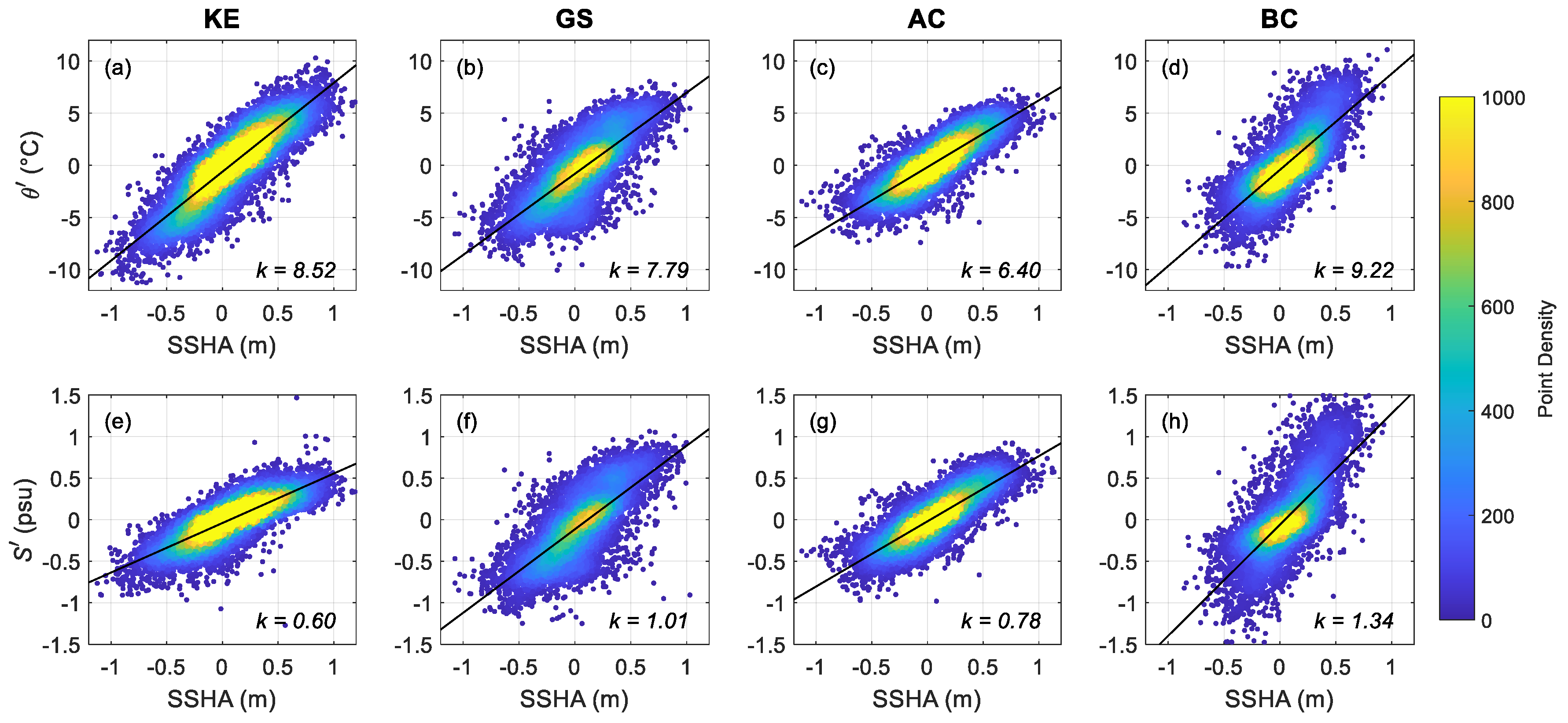
In order to further study the vertical thermohaline changes caused by eddy activities in the four WBCs, the correlation analysis of the maximum vertical thermohaline signals and SSHA signals of mesoscale eddies is given for each WBC, and the results are shown in Figure 9. The maximum vertical temperature or salinity signal of an eddy is the value of the eddy θ′ or S′ profile at the depth of the maximum mean θ′ or S′ profile of all eddies in Figure 8. In the mesoscale eddies, the vertical thermohaline signals have a good consistency with the SSHA signals for all four WBCs; the large eddy SSHA signals correspond to the large temperature and salinity anomalies. Based on the scatterplots of SSHA signals and maximum vertical thermohaline signals of eddies, the linear regression coefficients k of the scatterplots are calculated. In comparison, the regression coefficient k(θ′/SSHA) of eddies is the largest (about 9.2 °C/m) in the BC region and the smallest (about 6.2 °C/m) in the AC region, and the values are 8.5 °C/m and 7.8 °C/m in the KE and GS region, respectively. This suggests that mesoscale eddies with the same intensity can cause large vertical temperature changes in the BC region, but small changes in the AC region due to the deep thermoclines of water masses there. In terms of the regression coefficient k(S′/SSHA) of eddies, the value is the largest in the BC region and the smallest in the KE region. These all indicate that there are significant regional variations in the vertical thermohaline changes and the SSHA signals of mesoscale eddies, which are mainly influenced by local eddy strengths and the characteristics of water masses in different WBCs.
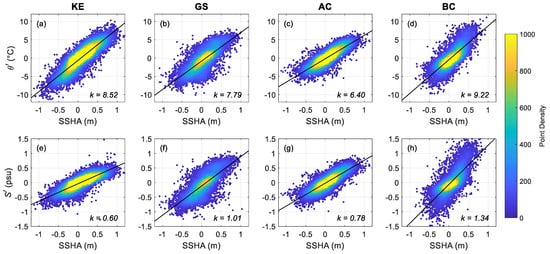
Figure 9.
(a–d) The scatterplots of SSHA signals and maximum vertical temperature anomaly θ′ of eddies, (e–h) the scatterplots of SSHA signals and maximum vertical salinity anomaly S′ of eddies in the four WBCs. The maximum vertical θ′ or S′ of an eddy is the value of the eddy θ′ or S′ profile at the depth of maximum mean θ′ or S′ profile of all eddies in Figure 8. Colors indicate the point density, the black lines are the linear regression of the scatterplots, and the regression coefficients k(θ′/SSHA) and k(S′/SSHA) are labeled in the figure.
5. Conclusions
Oceanic mesoscale eddies are abundant and vigorous in the four major WBC regions, i.e., the KE, GS, AC, and BC. Based on long time series of satellite altimeter data, the eddy identification and tracking show that eddies with long lifetimes and distances in the WBCs have a westward propagation trend, especially for the KE, GS, and AC regions. Eddies in the BC region are largely confined to the Brazil–Malvinas confluence and advected by the Malvinas Current and the Zapiola Drift. Eddies in the WBCs are clustered along the mainstream axis with anticyclonic preference in the pole-ward side and cyclonic preference in the equator-ward side. The GS eddies have the largest amplitude and BC eddies have the smallest amplitude.
Combining the altimeter-detected eddy results with the simultaneous observations of sea surface temperature, salinity, density, and chlorophyll concentration, the local impacts of eddy activities in each WBC were also analyzed. The eddy surface temperature and salinity signals are positively correlated with the eddy SSHA signal, while the eddy surface density and chlorophyll concentration are negatively correlated with the eddy SSHA signal. The correlation analysis of eddy surface signals in the WBCs reveals that eddies have regional differences in the surface signal changes of eddy activities. The different magnitudes of eddy surface signals in the four WBCs imply that eddies in different regions may have different contributions to eddy–atmosphere interactions. The large coefficient k(SSTA/SSHA) in the BC region explains that BC eddies have the largest SSTA signals, although their mean eddy amplitude is the smallest among the four WBCs. Based on the subsurface temperature and salinity information provided by Argo profiles, the analysis of the vertical thermohaline characteristics of mesoscale eddies in the four WBCs was carried out. The maximum eddy θ′ values in the KE and GS regions are ±2 °C, with the corresponding depths at 400 dbar and 600 dbar, respectively. The maximum eddy θ′ values in the AC and BC regions are about ±1.5 °C, with the corresponding depths at 500 dbar and 200 dbar. In the GS region, the mean vertical profiles of eddy S′ have a single sign from the surface to the deep ocean. In contrast, below a certain depth in the other three WBCs, the signs of eddy S′ are reversed to the upper layers. Eddies in the four WBCs have deep influence depths on the vertical thermohaline characteristics of water masses, which is not only related to the strong eddy activities but also to the thick thermoclines and haloclines of water masses in the WBCs. The different thermohaline characteristics of eddies in the four WBCs indicate that the heat and salt carried within the eddies are different in different regions, which is critical for the estimation of eddy-induced heat and salt transport in different regions.
In this study, the analysis of mesoscale eddy properties in the four WBCs is based on 30 years of merged SSHA data from multisource along-track altimeters. Considering that high-spatial-resolution altimetry satellites (e.g., SWOT, with a radar interferometer, which was launched in December 2022) will be available in the future to observe mesoscale/submesoscale dynamical processes, more abundant information about oceanic eddies can be obtained, which may further improve our understanding of eddy activities in the western boundary current. Moreover, this work only analyzes the climatic-mean state of eddy effect on surface temperature, salinity, density, and chlorophyll concentration, as well as the sub-surface thermohaline structure. Further studies on the seasonal and interannual variabilities of eddy effect, eddy–atmosphere interactions, interactions with other ocean currents, and eddy-induced heat and salt transport could be valuable in the four WBCs.
Author Contributions
J.Y. and C.Z. designed the experiments and W.C. carried them out. W.C. performed the data processing and analysis, plotted the figures, and wrote the manuscript. C.Z. led the research and improved the manuscript. All authors have read and agreed to the published version of the manuscript.
Funding
This research was funded by the Hainan Provincial Joint Project of Sanya Yazhou Bay Science and Technology City (2021CXLH0019), the National Natural Science Foundation of China (42106178 and 62231028), and the Science Foundation of Donghai Laboratory (DH-2022KF01014).
Data Availability Statement
The multi-altimeter merged SSHA product (SEALEVEL_GLO_PHY_L4_MY_008_047, https://doi.org/10.48670/moi-00148, accessed on 12 June 2023), the multi-observation global ocean SSS and SSD product (MULTIOBS_GLO_PHY_S_SURFACE_MYNRT_015_013, https://doi.org/10.48670/moi-00051, accessed on 6 August 2023), and the global ocean color product (OCEANCOLOUR_GLO_BGC_L4_MY_009_104, https://doi.org/10.48670/moi-00281, accessed on 15 November 2023) are distributed by the European Copernicus Marine Environment Monitoring Service (CMEMS). The daily OISST product Version 2.1 from AVHRR is provided by NOAA (https://doi.org/10.25921/RE9P-PT57 or https://data.nodc.noaa.gov, accessed on 15 November 2023). The Argo profiles are provided by Coriolis Global Data Acquisition Center of France (https://doi.org/10.17882/42182 or https://data-argo.ifremer.fr/ accessed on 20 October 2023). The World Ocean Atlas 2023 is provided by National Centers for Environmental Information, NOAA (https://www.ncei.noaa.gov/access/world-ocean-atlas-2023/, accessed on 16 March 2024).
Acknowledgments
The authors acknowledge all the data providers for the data utilized in this study.
Conflicts of Interest
The authors declare no conflicts of interest.
References
- Fu, L.-L.; Cazenave, A. Satellite Altimetry and Earth Sciences: A Handbook of Techniques and Applications (Google EBook). In Satellite Altimetry and Earth Sciences A Handbook of Techniques and Applications; Academic Press: Cambridge, MA, USA, 2000. [Google Scholar]
- Chelton, D.B.; Schlax, M.G.; Samelson, R.M. Global Observations of Nonlinear Mesoscale Eddies. Prog. Oceanogr. 2011, 91, 167–216. [Google Scholar] [CrossRef]
- Faghmous, J.H.; Frenger, I.; Yao, Y.; Warmka, R.; Lindell, A.; Kumar, V. A Daily Global Mesoscale Ocean Eddy Dataset from Satellite Altimetry. Sci. Data 2015, 2, 150028. [Google Scholar] [CrossRef]
- Dong, C.; Liu, L.; Nencioli, F.; Bethel, B.J.; Liu, Y.; Xu, G.; Ma, J.; Ji, J.; Sun, W.; Shan, H.; et al. The Near-Global Ocean Mesoscale Eddy Atmospheric-Oceanic-Biological Interaction Observational Dataset. Sci. Data 2022, 9, 436. [Google Scholar] [CrossRef]
- Ferrari, R.; Wunsch, C. Ocean Circulation Kinetic Energy: Reservoirs, Sources, and Sinks. Annu. Rev. Fluid Mech. 2009, 41, 253–282. [Google Scholar] [CrossRef]
- Zhang, Z.; Wang, W.; Qiu, B. Oceanic Mass Transport by Mesoscale Eddies. Science 2014, 345, 322–324. [Google Scholar] [CrossRef]
- Xu, C.; Shang, X.D.; Huang, R.X. Estimate of Eddy Energy Generation/Dissipation Rate in the World Ocean from Altimetry Data. Ocean Dyn. 2011, 61, 525–541. [Google Scholar] [CrossRef]
- Klein, P.; Lapeyre, G. The Oceanic Vertical Pump Induced by Mesoscale and Submesoscale Turbulence. Annu. Rev. Mar. Sci. 2009, 1, 351–375. [Google Scholar] [CrossRef]
- McGillicuddy, D.J. Mechanisms of Physical-Biological-Biogeochemical Interaction at the Oceanic Mesoscale. Annu. Rev. Mar. Sci. 2016, 8, 125–159. [Google Scholar] [CrossRef] [PubMed]
- Xu, L.; Li, P.; Xie, S.P.; Liu, Q.; Liu, C.; Gao, W. Observing Mesoscale Eddy Effects on Mode-Water Subduction and Transport in the North Pacific. Nat. Commun. 2016, 7, 10505. [Google Scholar] [CrossRef]
- Mathis, J.T.; Pickart, R.S.; Hansell, D.A.; Kadko, D.; Bates, N.R. Eddy Transport of Organic Carbon and Nutrients from the Chukchi Shelf: Impact on the Upper Halocline of the Western Arctic Ocean. J. Geophys. Res. Oceans 2007, 112, C05011. [Google Scholar] [CrossRef]
- Dong, C.; McWilliams, J.C.; Liu, Y.; Chen, D. Global Heat and Salt Transports by Eddy Movement. Nat. Commun. 2014, 5, 3294. [Google Scholar] [CrossRef] [PubMed]
- Maúre, E.R.; Ishizaka, J.; Sukigara, C.; Mino, Y.; Aiki, H.; Matsuno, T.; Tomita, H.; Goes, J.I.; Gomes, H.R. Mesoscale Eddies Control the Timing of Spring Phytoplankton Blooms: A Case Study in the Japan Sea. Geophys. Res. Lett. 2017, 44, 11115–11124. [Google Scholar] [CrossRef]
- Bian, C.; Jing, Z.; Wang, H.; Wu, L.; Chen, Z.; Gan, B.; Yang, H. Oceanic Mesoscale Eddies as Crucial Drivers of Global Marine Heatwaves. Nat. Commun. 2023, 14, 2970. [Google Scholar] [CrossRef]
- Zu, Y.; Fang, Y.; Sun, S.; Gao, L.; Yang, Y.; Guo, G. Seasonal Variation of Mesoscale Eddy Intensity in the Global Ocean. Acta Oceanol. Sin. 2024, 43, 48–58. [Google Scholar] [CrossRef]
- Zhai, X.; Johnson, H.L.; Marshall, D.P. Significant Sink of Ocean-Eddy Energy near Western Boundaries. Nat. Geosci. 2010, 3, 608–612. [Google Scholar] [CrossRef]
- Tang, B.; Hou, Y.; Yin, Y.; Hu, P. Probability Distributions of Statistical Characteristics of Mesoscale Eddies in the Global Ocean. Int. J. Remote Sens. 2019, 40, 6283–6297. [Google Scholar] [CrossRef]
- Richardson, P.L. Gulf Stream Rings. In Eddies in Marine Science; Robinson, A.R., Ed.; Springer: Berlin/Heidelberg, Germany, 1983; pp. 19–45. [Google Scholar]
- Talley, L.D.; Pickard, G.L.; Emery, W.J.; Swift, J.H. Descriptive Physical Oceanography: An Introduction, 6th ed.; Academic Press: Cambridge, MA, USA, 2011. [Google Scholar]
- Beal, L.M.; Bryden, H.L. The Velocity and Vorticity Structure of the Agulhas Current at 32°S. J. Geophys. Res. Oceans 1999, 104, 5151–5176. [Google Scholar] [CrossRef]
- Beal, L.M.; Elipot, S.; Houk, A.; Leber, G.M. Capturing the Transport Variability of a Western Boundary Jet: Results from the Agulhas Current Time-Series Experiment (ACT). J. Phys. Oceanogr. 2015, 45, 1302–1324. [Google Scholar] [CrossRef]
- Beal, L.M.; De Ruijter, W.P.M.; Biastoch, A.; Zahn, R.; Cronin, M.; Hermes, J.; Lutjeharms, J.; Quartly, G.; Tozuka, T.; Baker-Yeboah, S.; et al. On the Role of the Agulhas System in Ocean Circulation and Climate. Nature 2011, 472, 429–436. [Google Scholar] [CrossRef]
- Lutjeharms, J.R.E.; Van Ballegooyen, R.C. The Retroflection of the Agulhas Current. J. Phys. Oceanogr. 1988, 18, 1570–1583. [Google Scholar] [CrossRef]
- Richardson, P.L. Agulhas Leakage into the Atlantic Estimated with Subsurface Floats and Surface Drifters. Deep Sea Res. Part I Oceanogr. Res. Pap. 2007, 54, 1361–1389. [Google Scholar] [CrossRef]
- Wei, L.; Wang, C. Characteristics of Ocean Mesoscale Eddies in the Agulhas and Tasman Leakage Regions from Two Eddy Datasets. Deep Sea Res. Part II Top. Stud. Oceanogr. 2023, 208, 105264. [Google Scholar] [CrossRef]
- Xia, Q.; Dong, C.; He, Y.; Li, G.; Dong, J. Lagrangian Study of Several Long-Lived Agulhas Rings. J. Phys. Oceanogr. 2022, 52, 1049–1072. [Google Scholar] [CrossRef]
- Storer, B.A.; Buzzicotti, M.; Khatri, H.; Griffies, S.M.; Aluie, H. Global Energy Spectrum of the General Oceanic Circulation. Nat. Commun. 2022, 13, 5314. [Google Scholar] [CrossRef] [PubMed]
- Kang, D.; Curchitser, E.N. Energetics of Eddy-Mean Flow Interactions in the Gulf Stream Region. J. Phys. Oceanogr. 2015, 45, 1103–1120. [Google Scholar] [CrossRef]
- Waterman, S.; Hogg, N.G.; Jayne, S.R. Eddy-Mean Flow Interaction in the Kuroshio Extension Region. J. Phys. Oceanogr. 2011, 41, 1182–1208. [Google Scholar] [CrossRef]
- Adeagbo, O.S.; Du, Y.; Wang, T.; Wang, M. Eddy–Mean Flow Interactions in the Agulhas Leakage Region. J. Oceanogr. 2022, 78, 151–161. [Google Scholar] [CrossRef]
- Qiu, B.; Chen, S. Eddy-Mean Flow Interaction in the Decadally Modulating Kuroshio Extension System. Deep Sea Res. Part II Top. Stud. Oceanogr. 2010, 57, 1098–1110. [Google Scholar] [CrossRef]
- Ma, X.; Jing, Z.; Chang, P.; Liu, X.; Montuoro, R.; Small, R.J.; Bryan, F.O.; Greatbatch, R.J.; Brandt, P.; Wu, D.; et al. Western Boundary Currents Regulated by Interaction between Ocean Eddies and the Atmosphere. Nature 2016, 535, 533–537. [Google Scholar] [CrossRef]
- Garzoli, S.L.; Garraffo, Z. Transports, Frontal Motions and Eddies at the Brazil-Malvinas Currents Confluence. Deep. Sea Res. Part A Oceanogr. Res. Pap. 1989, 36, 681–703. [Google Scholar] [CrossRef]
- Leyba, I.M.; Saraceno, M.; Solman, S.A. Air-Sea Heat Fluxes Associated to Mesoscale Eddies in the Southwestern Atlantic Ocean and Their Dependence on Different Regional Conditions. Clim. Dyn. 2017, 49, 2491–2501. [Google Scholar] [CrossRef]
- Mason, E.; Pascual, A.; Gaube, P.; Ruiz, S.; Pelegrí, J.L.; Delepoulle, A. Subregional Characterization of Mesoscale Eddies across the Brazil-Malvinas Confluence. J. Geophys. Res. Oceans 2017, 122, 3329–3357. [Google Scholar] [CrossRef]
- Fu, L.L. Pattern and Velocity of Propagation of the Global Ocean Eddy Variability. J. Geophys. Res. Oceans 2009, 114, C11017. [Google Scholar] [CrossRef]
- Peng, L.; Chen, G.; Guan, L.; Tian, F. Contrasting Westward and Eastward Propagating Mesoscale Eddies in the Global Ocean. IEEE Trans. Geosci. Remote Sens. 2022, 60, 4504710. [Google Scholar] [CrossRef]
- Ni, Q.; Zhai, X.; Wang, G.; Marshall, D.P. Random Movement of Mesoscale Eddies in the Global Ocean. J. Phys. Oceanogr. 2020, 50, 2341–2357. [Google Scholar] [CrossRef]
- Itoh, S.; Yasuda, I. Water Mass Structure of Warm and Cold Anticyclonic Eddies in the Western Boundary Region of the Subarctic North Pacific. J. Phys. Oceanogr. 2010, 40, 2624–2642. [Google Scholar] [CrossRef]
- Cui, W.; Yang, J.; Jia, Y.; Zhang, J. Oceanic Eddy Detection and Analysis from Satellite-Derived SSH and SST Fields in the Kuroshio Extension. Remote Sens. 2022, 14, 5776. [Google Scholar] [CrossRef]
- Kang, D.; Curchitser, E.N. Gulf Stream Eddy Characteristics in a High-Resolution Ocean Model. J. Geophys. Res. Oceans 2013, 118, 4474–4487. [Google Scholar] [CrossRef]
- Cheng, Y.H.; Ho, C.R.; Zheng, Q.; Kuo, N.J. Statistical Characteristics of Mesoscale Eddies in the North Pacific Derived from Satellite Altimetry. Remote Sens. 2014, 6, 5164–5183. [Google Scholar] [CrossRef]
- Qiu, B. Kuroshio Extension Variability and Forcing of the Pacific Decadal Oscillations: Responses and Potential Feedback. J. Phys. Oceanogr. 2003, 33, 2465–2482. [Google Scholar] [CrossRef]
- Ji, J.; Dong, C.; Zhang, B.; Liu, Y.; Zou, B.; King, G.P.; Xu, G.; Chen, D. Oceanic Eddy Characteristics and Generation Mechanisms in the Kuroshio Extension Region. J. Geophys. Res. Oceans 2018, 123, 8548–8567. [Google Scholar] [CrossRef]
- Yang, C.; Yang, H.; Chen, Z.; Gan, B.; Liu, Y.; Wu, L. Seasonal Variability of Eddy Characteristics and Energetics in the Kuroshio Extension. Ocean Dyn. 2023, 73, 531–544. [Google Scholar] [CrossRef]
- Dong, D.; Brandt, P.; Chang, P.; Schütte, F.; Yang, X.; Yan, J.; Zeng, J. Mesoscale Eddies in the Northwestern Pacific Ocean: Three-Dimensional Eddy Structures and Heat/Salt Transports. J. Geophys. Res. Oceans 2017, 122, 9795–9813. [Google Scholar] [CrossRef]
- Sun, W.; Dong, C.; Wang, R.; Liu, Y.; Yu, K. Vertical Structure Anomalies of Oceanic Eddies in the Kuroshio Extension Region. J. Geophys. Res. Oceans 2017, 122, 1476–1496. [Google Scholar] [CrossRef]
- Yao, H.; Ma, C.; Jing, Z.; Zhang, Z. On the Vertical Structure of Mesoscale Eddies in the Kuroshio-Oyashio Extension. Geophys. Res. Lett. 2023, 50, e2023GL105642. [Google Scholar] [CrossRef]
- Zhang, S.; Curchitser, E.N.; Kang, D.; Stock, C.A.; Dussin, R. Impacts of Mesoscale Eddies on the Vertical Nitrate Flux in the Gulf Stream Region. J. Geophys. Res. Oceans 2018, 123, 497–513. [Google Scholar] [CrossRef]
- Gaube, P.; McGillicuddy, D.J. The Influence of Gulf Stream Eddies and Meanders on Near-Surface Chlorophyll. Deep Sea Res. Part I Oceanogr. Res. Pap. 2017, 122, 1–16. [Google Scholar] [CrossRef]
- Gaube, P.; McGillicuddy, D.J.; Chelton, D.B.; Behrenfeld, M.J.; Strutton, P.G. Regional Variations in the Influence of Mesoscale Eddies on Near-Surface Chlorophyll. J. Geophys. Res. Oceans 2014, 119, 8195–8220. [Google Scholar] [CrossRef]
- Wang, X.; Zhang, S.; Lin, X.; Qiu, B.; Yu, L. Characteristics of 3-Dimensional Structure and Heat Budget of Mesoscale Eddies in the South Atlantic Ocean. J. Geophys. Res. Oceans 2021, 126, e2020JC016922. [Google Scholar] [CrossRef]
- Laxenaire, R.; Speich, S.; Blanke, B.; Chaigneau, A.; Pegliasco, C.; Stegner, A. Anticyclonic Eddies Connecting the Western Boundaries of Indian and Atlantic Oceans. J. Geophys. Res. Oceans 2018, 123, 7651–7677. [Google Scholar] [CrossRef]
- Nencioli, F.; Dall’Olmo, G.; Quartly, G.D. Agulhas Ring Transport Efficiency From Combined Satellite Altimetry and Argo Profiles. J. Geophys. Res. Oceans 2018, 123, 5874–5888. [Google Scholar] [CrossRef]
- Pilo, G.S.; Mata, M.M.; Azevedo, J.L.L. Eddy Surface Properties and Propagation at Southern Hemisphere Western Boundary Current Systems. Ocean Sci. 2015, 11, 629–641. [Google Scholar] [CrossRef]
- Halo, I.; Raj, R.P. Comparative Oceanographic Eddy Variability During Climate Change in the Agulhas Current and Somali Coastal Current Large Marine Ecosystems. Environ. Dev. 2020, 36, 100586. [Google Scholar] [CrossRef]
- Rykova, T.; Oke, P.R.; Griffin, D.A. A Comparison of the Structure, Properties, and Water Mass Composition of Quasi-Isotropic Eddies in Western Boundary Currents in an Eddy-Resolving Ocean Model. Ocean Model. 2017, 114, 1–13. [Google Scholar] [CrossRef]
- Saraceno, M.; Provost, C. On Eddy Polarity Distribution in the Southwestern Atlantic. Deep Sea Res. Part I Oceanogr. Res. Pap. 2012, 69, 62–69. [Google Scholar] [CrossRef]
- Pujol, M.I. PRODUCT USER MANUAL. For Sea Level Altimeter Products (Issue: 8.0); CMEMS-SL-PUM-008-032-062; MERCATOR OCEAN: Toulouse, France, 2023. [Google Scholar]
- Huang, B.; Liu, C.; Banzon, V.; Freeman, E.; Graham, G.; Hankins, B.; Smith, T.; Zhang, H.M. Improvements of the Daily Optimum Interpolation Sea Surface Temperature (DOISST) Version 2.1. J. Clim. 2021, 34, 2923–2939. [Google Scholar] [CrossRef]
- Reynolds, R.W.; Smith, T.M.; Liu, C.; Chelton, D.B.; Casey, K.S.; Schlax, M.G. Daily High-Resolution-Blended Analyses for Sea Surface Temperature. J. Clim. 2007, 20, 5473–5496. [Google Scholar] [CrossRef]
- Sammartino, M.; Aronica, S.; Santoleri, R.; Nardelli, B.B. Retrieving Mediterranean Sea Surface Salinity Distribution and Interannual Trends from Multi-Sensor Satellite and In Situ Data. Remote Sens. 2022, 14, 2502. [Google Scholar] [CrossRef]
- Colella, S.; Böhm, E.; Cesarini, C.; Garnesson, P.; Netting, J.; Calton, B. PRODUCT USER MANUAL. For Ocean Colour Products (Issue: 4.0); MERCATOR OCEAN: Toulouse, France, 2023. [Google Scholar]
- Chaigneau, A.; Le Texier, M.; Eldin, G.; Grados, C.; Pizarro, O. Vertical Structure of Mesoscale Eddies in the Eastern South Pacific Ocean: A Composite Analysis from Altimetry and Argo Profiling Floats. J. Geophys. Res. Oceans 2011, 116, C11025. [Google Scholar] [CrossRef]
- Yang, G.; Wang, F.; Li, Y.; Lin, P. Mesoscale Eddies in the Northwestern Subtropical Pacific Ocean: Statistical Characteristics and Three-Dimensional Structures. J. Geophys. Res. Oceans 2013, 118, 1906–1925. [Google Scholar] [CrossRef]
- Reagan, J.R.; Garcia, H.E.; Boyer, T.P.; Baranova, O.K.; Bouchard, C.; Cross, S.L.; Dukhovskoy, D.; Grodsky, A.I.; Locarnini, R.A.; Mishonov, A.V.; et al. World Ocean Atlas 2023: Product Documentation; Ocean Climate Laboratory: Silver Spring, MD, USA, 2024. [Google Scholar]
- Chaigneau, A.; Gizolme, A.; Grados, C. Mesoscale Eddies off Peru in Altimeter Records: Identification Algorithms and Eddy Spatio-Temporal Patterns. Prog. Oceanogr. 2008, 79, 106–119. [Google Scholar] [CrossRef]
- Souza, J.M.A.C.; De Boyer Montégut, C.; Le Traon, P.Y. Comparison Between Three Implementations of Automatic Identification Algorithms for the Quantification and Characterization of Mesoscale Eddies in the South Atlantic Ocean. Ocean Sci. 2011, 7, 317–334. [Google Scholar] [CrossRef]
- Roman-Stork, H.L.; Byrne, D.A.; Leuliette, E.W. MESI: A Multiparameter Eddy Significance Index. Earth Space Sci. 2023, 10, e2022EA002583. [Google Scholar] [CrossRef]
- Ding, M.; Liu, H.; Lin, P.; Meng, Y.; Yu, Z. Evaluating Westward and Eastward Propagating Mesoscale Eddies Using a 1/10° Global Ocean Simulation of CAS-LICOM3. Ocean Model. 2024, 189, 102373. [Google Scholar] [CrossRef]
- Ueno, H.; Bracco, A.; Barth, J.A.; Budyansky, M.V.; Hasegawa, D.; Itoh, S.; Kim, S.Y.; Ladd, C.; Lin, X.; Park, Y.G.; et al. Review of Oceanic Mesoscale Processes in the North Pacific: Physical and Biogeochemical Impacts. Prog. Oceanogr. 2023, 212, 102955. [Google Scholar] [CrossRef]
- Itoh, S.; Yasuda, I. Characteristics of Mesoscale Eddies in the Kuroshio-Oyashio Extension Region Detected from the Distribution of the Sea Surface Height Anomaly. J. Phys. Oceanogr. 2010, 40, 1018–1034. [Google Scholar] [CrossRef]
- Morrow, R.; Birol, F.; Griffin, D.; Sudre, J. Divergent Pathways of Cylonic and Anti-Cyclonic Ocean Eddies. Geophys. Res. Lett. 2004, 31, 1–5. [Google Scholar] [CrossRef]
- Chen, G.; Chen, X.; Cao, C. Divergence and Dispersion of Global Eddy Propagation from Satellite Altimetry. J. Phys. Oceanogr. 2022, 52, 705–722. [Google Scholar] [CrossRef]
- Liu, Y.; Zheng, Q.; Li, X. Characteristics of Global Ocean Abnormal Mesoscale Eddies Derived From the Fusion of Sea Surface Height and Temperature Data by Deep Learning. Geophys. Res. Lett. 2021, 48, e2021GL094772. [Google Scholar] [CrossRef]
- Sun, W.; Dong, C.; Tan, W.; He, Y. Statistical Characteristics of Cyclonic Warm-Core Eddies and Anticyclonic Cold-Core Eddies in the North Pacific Based on Remote Sensing Data. Remote Sens. 2019, 11, 208. [Google Scholar] [CrossRef]
- Castelao, R.M. Mesoscale Eddies in the South Atlantic Bight and the Gulf Stream Recirculation Region: Vertical Structure. J. Geophys. Res. Oceans 2014, 119, 2048–2065. [Google Scholar] [CrossRef]
- Sun, W.; Dong, C.; Tan, W.; Liu, Y.; He, Y.; Wang, J. Vertical Structure Anomalies of Oceanic Eddies and Eddy-Induced Transports in the South China Sea. Remote Sens. 2018, 10, 795. [Google Scholar] [CrossRef]
- Zhang, Z.; Tian, J.; Qiu, B.; Zhao, W.; Chang, P.; Wu, D.; Wan, X. Observed 3D Structure, Generation, and Dissipation of Oceanic Mesoscale Eddies in the South China Sea. Sci. Rep. 2016, 6, 24349. [Google Scholar] [CrossRef] [PubMed]
- Cui, W.; Zhang, J.; Yang, J. Seasonal Variation in Eddy Activity and Associated Heat/Salt Transport in the Bay of Bengal Based on Satellite, Argo, and 3D Reprocessed Data. Ocean Sci. 2022, 18, 1645–1663. [Google Scholar] [CrossRef]
- Mason, E.; Ruiz, S.; Bourdalle-Badie, R.; Reffray, G.; García-Sotillo, M.; Pascual, A. New Insight into 3-D Mesoscale Eddy Properties from CMEMS Operational Models in the Western Mediterranean. Ocean Sci. 2019, 15, 1111–1131. [Google Scholar] [CrossRef]
- Yang, G.; Yu, W.; Yuan, Y.; Zhao, X.; Wang, F.; Chen, G.; Liu, L.; Duan, Y. Characteristics, Vertical Structures, and Heat/Salt Transports of Mesoscale Eddies in the Southeastern Tropical Indian Ocean. J. Geophys. Res. Oceans 2015, 120, 6733–6750. [Google Scholar] [CrossRef]
- Schütte, F.; Brandt, P.; Karstensen, J. Occurrence and Characteristics of Mesoscale Eddies in the Tropical Atlantic Ocean. Ocean Sci. 2016, 12, 663–685. [Google Scholar] [CrossRef]
- Amores, A.; Melnichenko, O.; Maximenko, N. Coherent Mesoscale Eddies in the North Atlantic Subtropical Gyre: 3-D Structure and Transport with Application to the Salinity Maximum. J. Geophys. Res. Oceans 2017, 122, 23–41. [Google Scholar] [CrossRef]
- Keppler, L.; Cravatte, S.; Chaigneau, A.; Pegliasco, C.; Gourdeau, L.; Singh, A. Observed Characteristics and Vertical Structure of Mesoscale Eddies in the Southwest Tropical Pacific. J. Geophys. Res. Oceans 2018, 123, 2731–2756. [Google Scholar] [CrossRef]
- Pegliasco, C.; Chaigneau, A.; Morrow, R. Main Eddy Vertical Structures Observed in the Four Major Eastern Boundary Upwelling Systems. J. Geophys. Res. Oceans 2015, 120, 6008–6033. [Google Scholar] [CrossRef]
- Chenillat, F.; Franks, P.J.S.; Capet, X.; Rivière, P.; Grima, N.; Blanke, B.; Combes, V. Eddy Properties in the Southern California Current System. Ocean Dyn. 2018, 68, 761–777. [Google Scholar] [CrossRef]

Disclaimer/Publisher’s Note: The statements, opinions and data contained in all publications are solely those of the individual author(s) and contributor(s) and not of MDPI and/or the editor(s). MDPI and/or the editor(s) disclaim responsibility for any injury to people or property resulting from any ideas, methods, instructions or products referred to in the content. |
© 2024 by the authors. Licensee MDPI, Basel, Switzerland. This article is an open access article distributed under the terms and conditions of the Creative Commons Attribution (CC BY) license (https://creativecommons.org/licenses/by/4.0/).