
Residual-Based Implicit Neural Representation for Synthetic Aperture Radar Images


Abstract
:1. Introduction
- We pioneer the exploration of continuous representation with INRs for SAR images, finding that INRs can benefit from first learning the intra-pixel independent mapping.
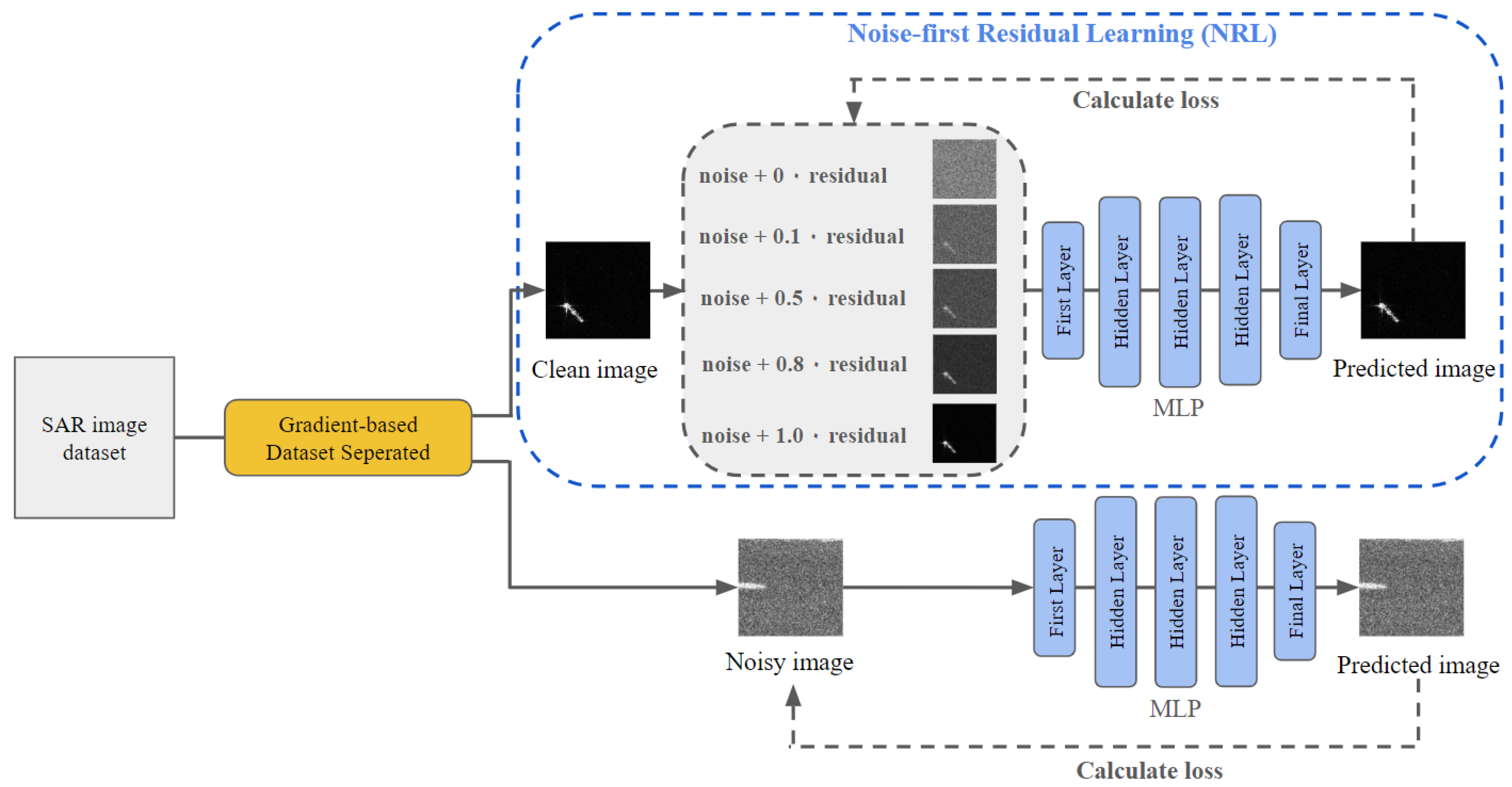
- We propose a noise-first residual learning process which first learns the uniform noise (intra-pixel independent mapping), then gradually incorporates the residual image (inter-pixel relationships) into the optimization target.
- Extensive experiments demonstrate that our noise-first residual learning approach significantly improves performance over multiple state-of-the-art INR baseline methods.
2. Related Work
2.1. Implict Neural Representation
2.2. Synthetic Aperture Radar Images
3. Background and Method
3.1. Background
3.2. Our Proposed Method
3.2.1. Noise-First Residual Learning for INR
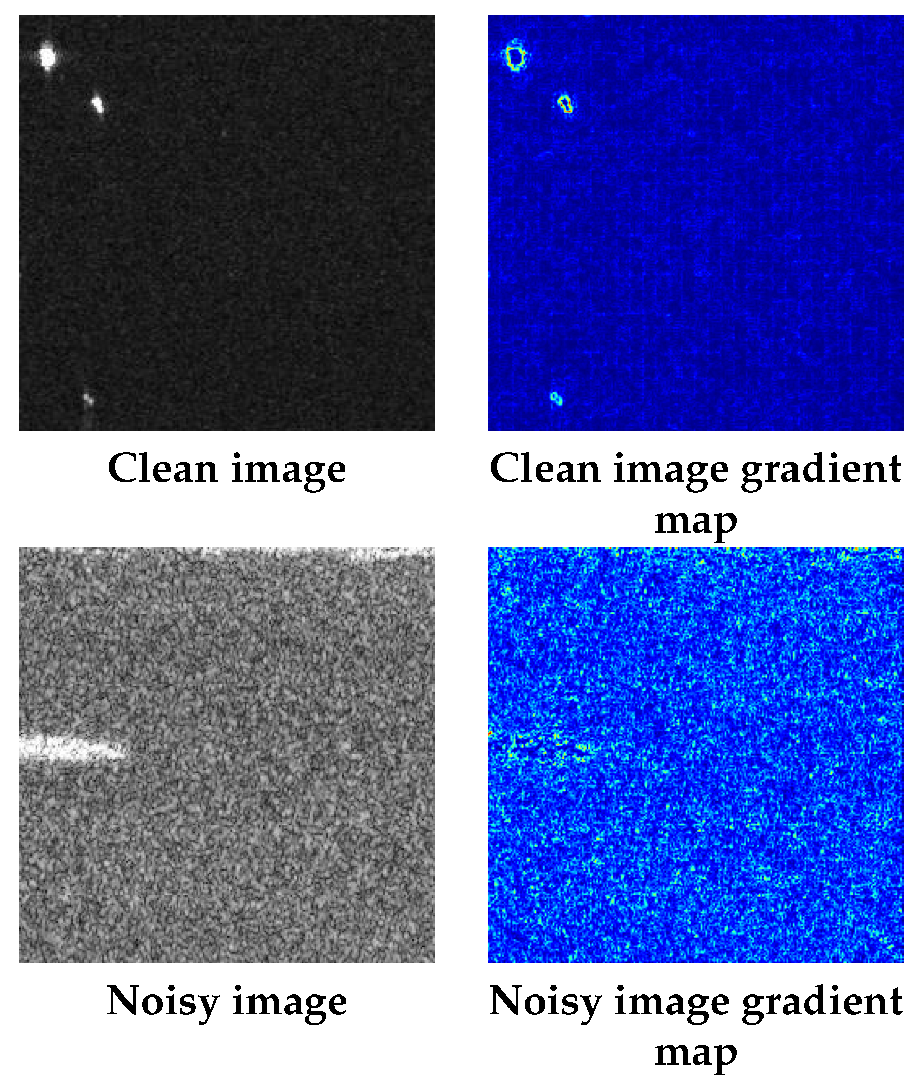
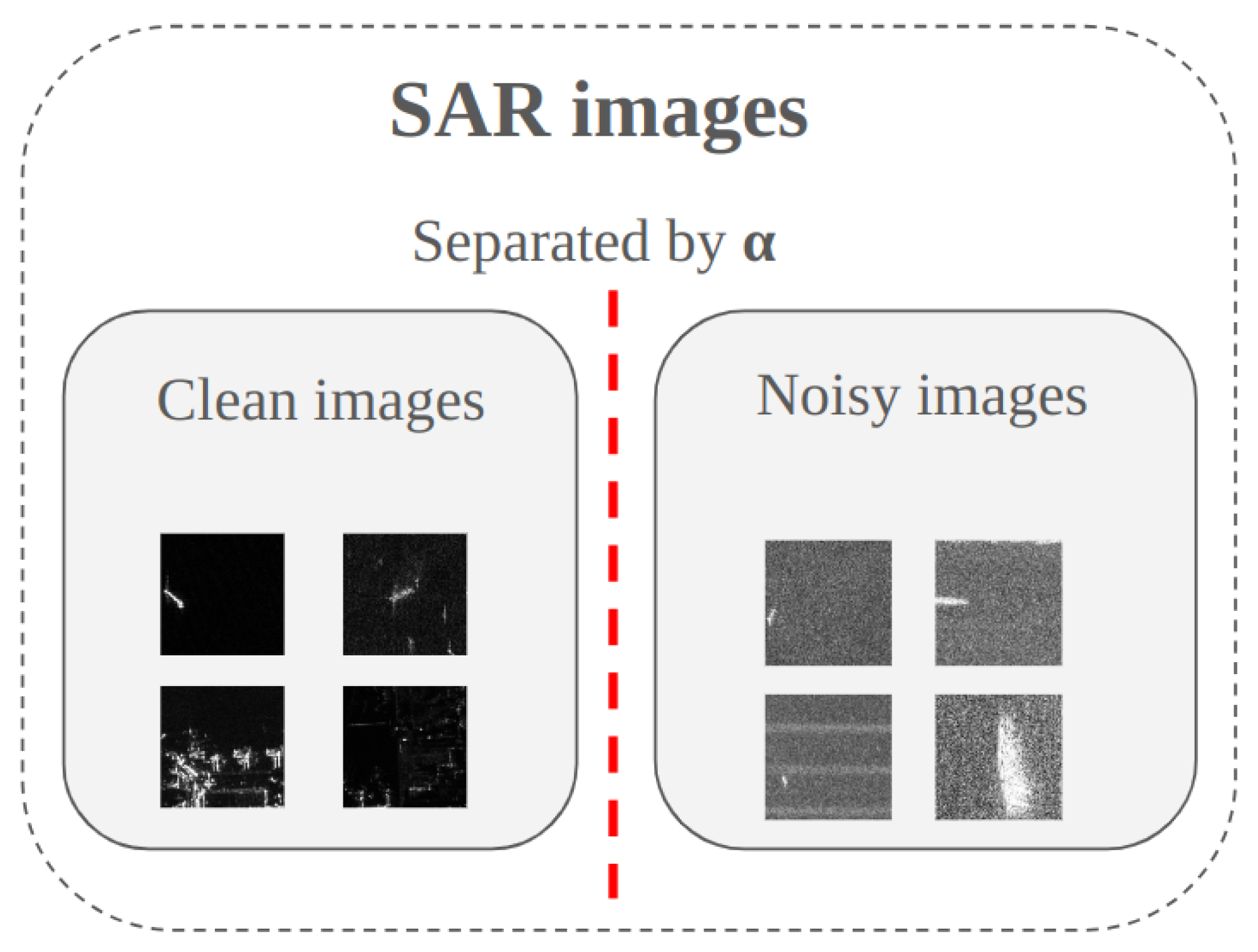
3.2.2. Gradient-Based Dataset Separation
4. Experiments
4.1. Implementation Details and Evaluation Metrics
4.2. SARDet-100K Dataset
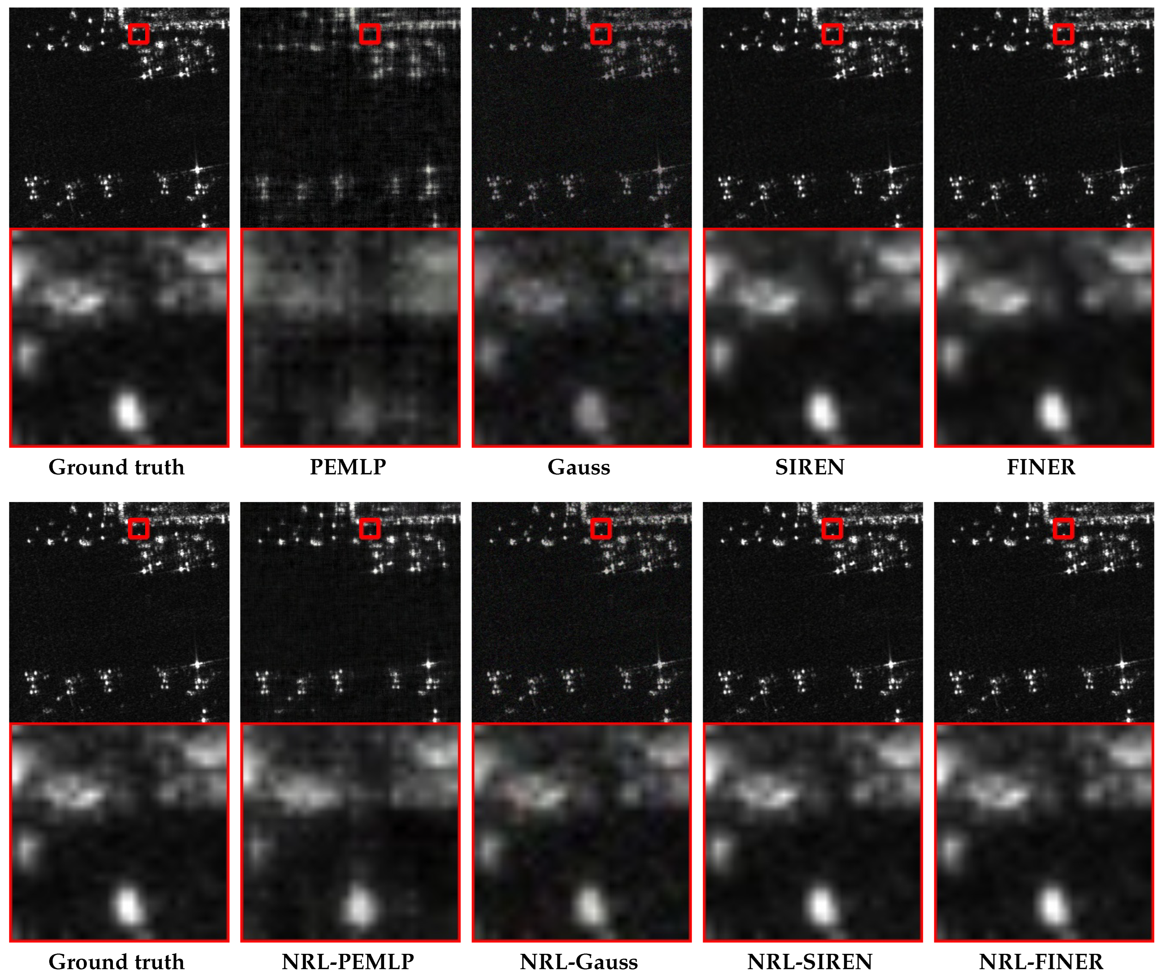
4.3. SAR Image Representation
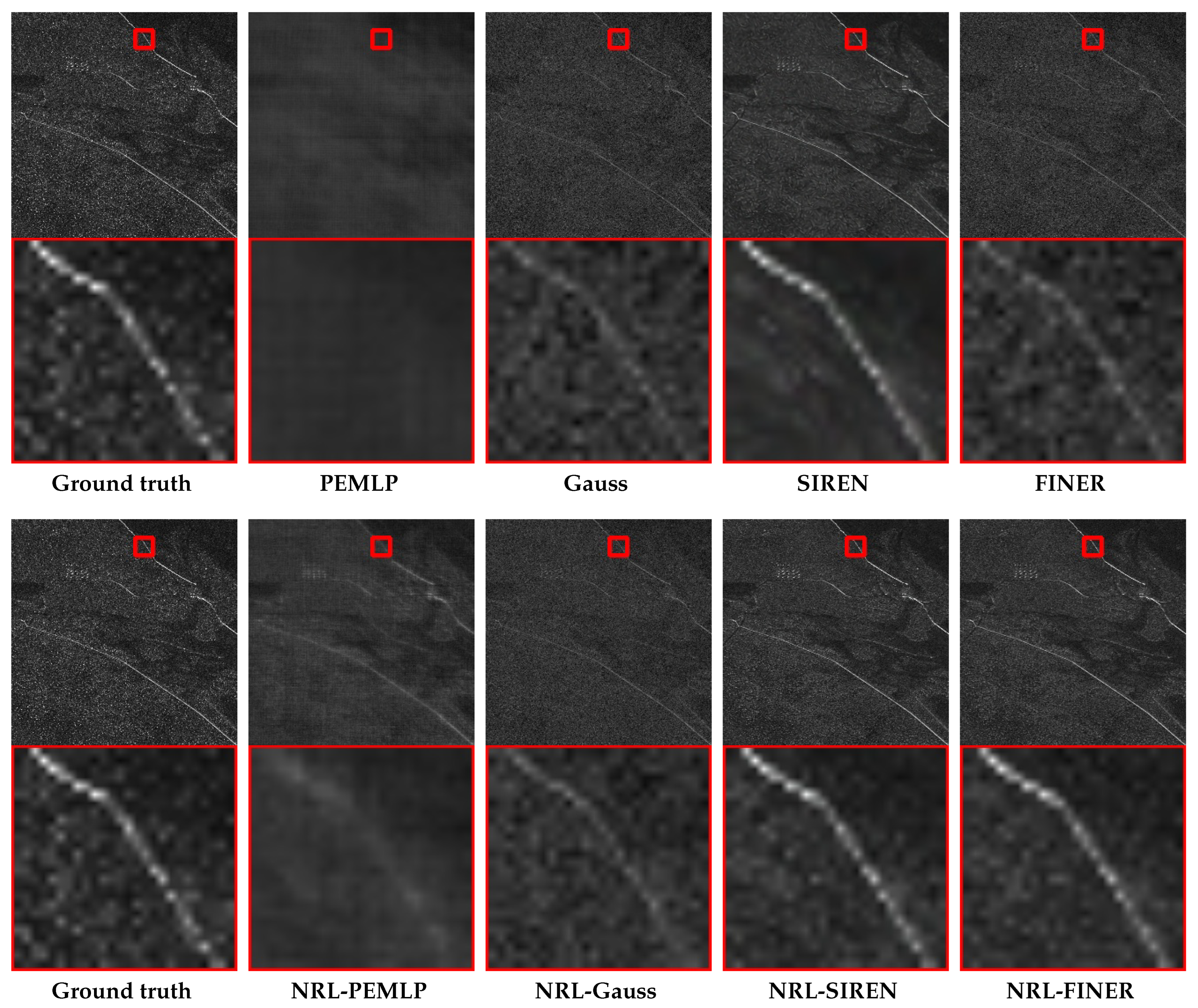
4.4. High-Resolution SAR Image Representation
4.5. Ablation Study
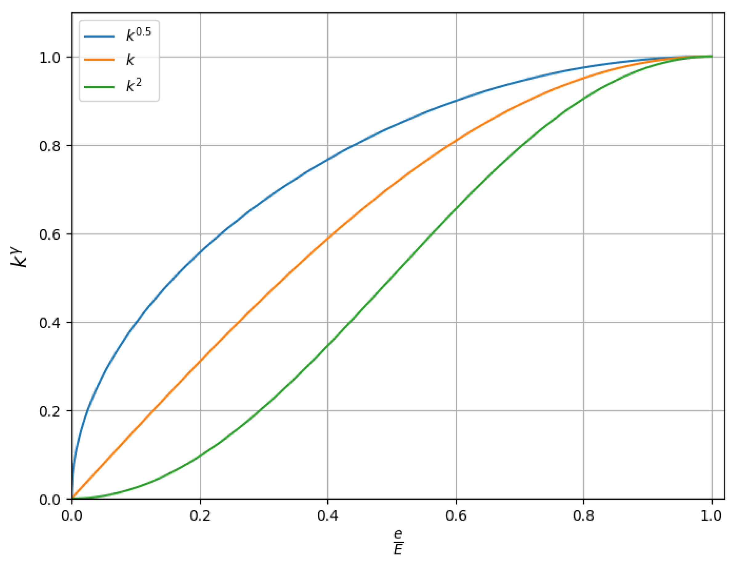
4.5.1. Ablation Study of Focusing Parameter
4.5.2. Ablation Study on Learning Epochs for Target Image
4.5.3. Ablation Study on Noise Level
5. Discussion
6. Conclusions
Author Contributions
Funding
Data Availability Statement
Acknowledgments
Conflicts of Interest
Abbreviations
| INRs | Implicit Neural Representations |
| SAR | Synthetic Aperture Radar |
| NRL | Noise-first Residual Learning |
| MLP | Multi-Layer Perceptron |
| MSE | Mean Squared Error |
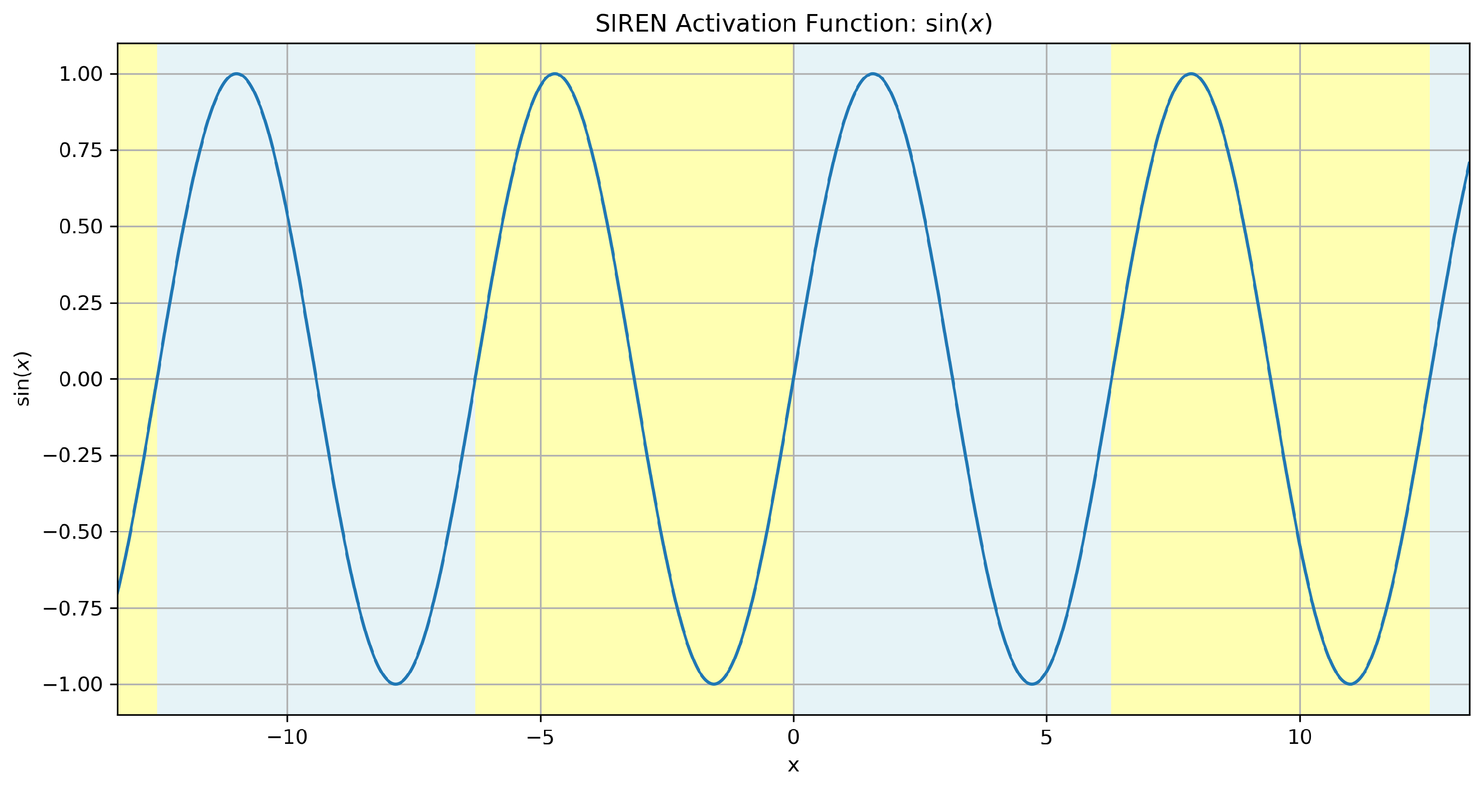
| SIREN | Sinusoidal Representation Network |
| PEMLP | Position Embedding Multi-Layer Perceptron |
| FINER | Flexible spectral-bias tuning in Implicit Neural Representation |
| WIRE | Wavelet Implicit Neural Representation |
| PSNR | Peak Signal-to-Noise Ratio |
| SSIM | Structural Similarity Index |
| MSFA | Multi-Stage Filter Augmentation |
| CNN | Convolutional Neural Network |
| ReLU | Rectified Linear Unit |
| HVS | Human Visual System |
References
- Park, J.J.; Florence, P.; Straub, J.; Newcombe, R.; Lovegrove, S. Deepsdf: Learning continuous signed distance functions for shape representation. In Proceedings of the IEEE/CVF conference on Computer Vision and Pattern Recognition, Long Beach, CA, USA, 15–20 June 2019; pp. 165–174. [Google Scholar]
- Mildenhall, B.; Srinivasan, P.P.; Tancik, M.; Barron, J.T.; Ramamoorthi, R.; Ng, R. Nerf: Representing scenes as neural radiance fields for view synthesis. Commun. ACM 2021, 65, 99–106. [Google Scholar] [CrossRef]
- Mescheder, L.; Oechsle, M.; Niemeyer, M.; Nowozin, S.; Geiger, A. Occupancy networks: Learning 3D reconstruction in function space. In Proceedings of the IEEE/CVF Conference on Computer Vision and Pattern Recognition, Long Beach, CA, USA, 15–20 June 2019; pp. 4460–4470. [Google Scholar]
- Molaei, A.; Aminimehr, A.; Tavakoli, A.; Kazerouni, A.; Azad, B.; Azad, R.; Merhof, D. Implicit neural representation in medical imaging: A comparative survey. In Proceedings of the IEEE/CVF International Conference on Computer Vision, Paris, France, 1–6 October 2023; pp. 2381–2391. [Google Scholar]
- Sitzmann, V.; Martel, J.N.; Bergman, A.W.; Lindell, D.B.; Wetzstein, G. Light field networks: Neural scene representations with single-evaluation rendering. Adv. Neural Inf. Process. Syst. 2021, 34, 19313–19325. [Google Scholar]
- Sitzmann, V.; Martel, J.; Bergman, A.; Lindell, D.; Wetzstein, G. Implicit neural representations with periodic activation functions. Adv. Neural Inf. Process. Syst. 2020, 33, 7462–7473. [Google Scholar]
- Rahaman, N.; Baratin, A.; Arpit, D.; Draxler, F.; Lin, M.; Hamprecht, F.; Bengio, Y.; Courville, A. On the spectral bias of neural networks. In Proceedings of the International Conference on Machine Learning, PMLR, Long Beach, CA, USA, 9–15 June 2019; pp. 5301–5310. [Google Scholar]
- Tancik, M.; Srinivasan, P.; Mildenhall, B.; Fridovich-Keil, S.; Raghavan, N.; Singhal, U.; Ramamoorthi, R.; Barron, J.; Ng, R. Fourier features let networks learn high frequency functions in low dimensional domains. Adv. Neural Inf. Process. Syst. 2020, 33, 7537–7547. [Google Scholar]
- Sitzmann, V.; Zollhöfer, M.; Wetzstein, G. Scene representation networks: Continuous 3d-structure-aware neural scene representations. Adv. Neural Inf. Process. Syst. 2019, 32. [Google Scholar]
- Martel, J.N.; Lindell, D.B.; Lin, Z.; Chan, E.R.; Wetzstein, G. ACORN: Adaptive coordinate networks for neural scene representation. arXiv 2021, arXiv:2104.09575. [Google Scholar] [CrossRef]
- Passah, A.; Sur, S.N.; Paul, B.; Kandar, D. SAR image classification: A comprehensive study and analysis. IEEE Access 2022, 10, 20385–20399. [Google Scholar] [CrossRef]
- Chen, S.; Wang, H. SAR target recognition based on deep learning. In Proceedings of the 2014 International Conference on Data Science and Advanced Analytics (DSAA), IEEE, Shanghai, China, 30 October–1 November 2014; pp. 541–547. [Google Scholar]
- Denis, L.; Dalsasso, E.; Tupin, F. A review of deep-learning techniques for SAR image restoration. In Proceedings of the 2021 IEEE International Geoscience and Remote Sensing Symposium IGARSS, IEEE, Brussels, Belgium, 11–16 July 2021; pp. 411–414. [Google Scholar]
- Skrunes, S.; Johansson, A.M.; Brekke, C. Synthetic aperture radar remote sensing of operational platform produced water releases. Remote Sens. 2019, 11, 2882. [Google Scholar] [CrossRef]
- Zhang, T.; Zeng, T.; Zhang, X. Synthetic aperture radar (SAR) meets deep learning. Remote Sens. 2023, 15, 303. [Google Scholar] [CrossRef]
- Lee, J.S.; Jurkevich, L.; Dewaele, P.; Wambacq, P.; Oosterlinck, A. Speckle filtering of synthetic aperture radar images: A review. Remote Sens. Rev. 1994, 8, 313–340. [Google Scholar] [CrossRef]
- Chierchia, G.; Scarpa, G.; Poggi, G.; Verdoliva, L.; Ciotola, M. Speckle2Void: Deep Self-Supervised SAR Despeckling with Blind-Spot Convolutional Neural Networks. IEEE Trans. Geosci. Remote Sens. 2021, 59, 9814–9826. [Google Scholar]
- Liu, K.; Liu, F.; Wang, H.; Ma, N.; Bu, J.; Han, B. Partition speeds up learning implicit neural representations based on exponential-increase hypothesis. In Proceedings of the IEEE/CVF International Conference on Computer Vision, Paris, France, 1–6 October 2023; pp. 5474–5483. [Google Scholar]
- Shen, L.; Pauly, J.; Xing, L. NeRP: Implicit neural representation learning with prior embedding for sparsely sampled image reconstruction. IEEE Trans. Neural Networks Learn. Syst. 2022, 35, 770–782. [Google Scholar] [CrossRef]
- Fang, W.; Tang, Y.; Guo, H.; Yuan, M.; Mok, T.C.; Yan, K.; Yao, J.; Chen, X.; Liu, Z.; Lu, L.; et al. CycleINR: Cycle Implicit Neural Representation for Arbitrary-Scale Volumetric Super-Resolution of Medical Data. In Proceedings of the IEEE/CVF Conference on Computer Vision and Pattern Recognition, Seattle, WA, USA, 16–22 June 2024; pp. 11631–11641. [Google Scholar]
- Rumelhart, D.E.; Hinton, G.E.; Williams, R.J. Learning representations by back-propagating errors. Nature 1986, 323, 533–536. [Google Scholar] [CrossRef]
- Chen, Z.; Zhang, H. Learning implicit fields for generative shape modeling. In Proceedings of the IEEE/CVF Conference on Computer Vision and Pattern Recognition, Long Beach, CA, USA, 15–20 June 2019; pp. 5939–5948. [Google Scholar]
- Genova, K.; Cole, F.; Sud, A.; Sarna, A.; Funkhouser, T. Deep structured implicit functions. arXiv 2019, arXiv:1912.06126. [Google Scholar]
- Niemeyer, M.; Mescheder, L.; Oechsle, M.; Geiger, A. Differentiable volumetric rendering: Learning implicit 3D representations without 3D supervision. In Proceedings of the IEEE/CVF Conference on Computer Vision and Pattern Recognition, Seattle, WA, USA, 14–19 June 2020; pp. 3504–3515. [Google Scholar]
- Liu, L.; Lin, W.; Bao, Y.; Bai, X.; Kavan, L.; Wu, J.; Tong, X. Neural sparse voxel fields. Adv. Neural Inf. Process. Syst. 2020, 33, 15651–15663. [Google Scholar]
- Xie, S.; Zhu, H.; Liu, Z.; Zhang, Q.; Zhou, Y.; Cao, X.; Ma, Z. DINER: Disorder-invariant implicit neural representation. In Proceedings of the IEEE/CVF Conference on Computer Vision and Pattern Recognition, Vancouver, BC, Canada, 17–24 June 2023; pp. 6143–6152. [Google Scholar]
- Saragadam, V.; LeJeune, D.; Tan, J.; Balakrishnan, G.; Veeraraghavan, A.; Baraniuk, R.G. Wire: Wavelet implicit neural representations. In Proceedings of the IEEE/CVF Conference on Computer Vision and Pattern Recognition, Vancouver, BC, Canada, 17–24 June 2023; pp. 18507–18516. [Google Scholar]
- Liu, Z.; Zhu, H.; Zhang, Q.; Fu, J.; Deng, W.; Ma, Z.; Guo, Y.; Cao, X. FINER: Flexible spectral-bias tuning in Implicit NEural Representation by Variable-periodic Activation Functions. In Proceedings of the IEEE/CVF Conference on Computer Vision and Pattern Recognition, Seattle, WA, USA, 16–22 June 2024; pp. 2713–2722. [Google Scholar]
- Chen, Z.; Zhang, K.; Gao, S.; Zhang, H.; Tong, X. MetaSDF: Meta-learning signed distance functions. Adv. Neural Inf. Process. Syst. 2022, 33, 10136–10147. [Google Scholar]
- Chen, A.; Xu, Z.; Geiger, A.; Yu, J.; Su, H. TensoRF: Tensorial radiance fields. arXiv 2022, arXiv:2203.09517. [Google Scholar]
- Schowengerdt, R.A. Remote Sensing: Models and Methods for Image Processing; Elsevier: Amsterdam, The Netherlands, 2006. [Google Scholar]
- Moreira, A.; Prats-Iraola, P.; Younis, M.; Krieger, G.; Hajnsek, I.; Papathanassiou, K.P. A tutorial on synthetic aperture radar. IEEE Geosci. Remote Sens. Mag. 2013, 1, 6–43. [Google Scholar] [CrossRef]
- Elachi, C.; Van Zyl, J.J. Introduction to the Physics and Techniques of Remote Sensing; John Wiley & Sons: Hoboken, NJ, USA, 2021. [Google Scholar]
- Navalgund, R.R.; Jayaraman, V.; Roy, P. Remote sensing applications: An overview. Curr. Sci. 2007, 93, 1747–1766. [Google Scholar]
- Monserrat, O.; Crosetto, M.; Luzi, G. A review of ground-based SAR interferometry for deformation measurement. ISPRS J. Photogramm. Remote Sens. 2014, 93, 40–48. [Google Scholar] [CrossRef]
- Wang, S.; He, F.; Dong, Z. A Novel Intrapulse Beamsteering SAR Imaging Mode Based on OFDM-Chirp Signals. Remote Sens. 2023, 16, 126. [Google Scholar] [CrossRef]
- Chang, Y.L.; Anagaw, A.; Chang, L.; Wang, Y.C.; Hsiao, C.Y.; Lee, W.H. Ship detection based on YOLOv2 for SAR imagery. Remote Sens. 2019, 11, 786. [Google Scholar] [CrossRef]
- Koo, V.; Chan, Y.K.; Vetharatnam, G.; Chua, M.Y.; Lim, C.H.; Lim, C.S.; Thum, C.; Lim, T.S.; bin Ahmad, Z.; Mahmood, K.A.; et al. A new unmanned aerial vehicle synthetic aperture radar for environmental monitoring. Prog. Electromagn. Res. 2012, 122, 245–268. [Google Scholar] [CrossRef]
- McNairn, H.; Shang, J. A review of multitemporal synthetic aperture radar (SAR) for crop monitoring. In Multitemporal Remote Sensing: Methods and Applications; Springer: Cham, Switzerland, 2016; pp. 317–340. [Google Scholar]
- Henderson, F.M.; Xia, Z.G. SAR applications in human settlement detection, population estimation and urban land use pattern analysis: A status report. IEEE Trans. Geosci. Remote Sens. 1997, 35, 79–85. [Google Scholar] [CrossRef]
- Melillos, G.; Themistocleous, K.; Papadavid, G.; Agapiou, A.; Kouhartsiouk, D.; Prodromou, M.; Michaelides, S.; Hadjimitsis, D.G. Using field spectroscopy combined with synthetic aperture radar (SAR) technique for detecting underground structures for defense and security applications in Cyprus. In Proceedings of the Detection and Sensing of Mines, Explosive Objects, and Obscured Targets XXII, SPIE, Anaheim, CA, USA, 10–12 April 2017; Volume 10182, pp. 23–35. [Google Scholar]
- Li, Y.; Li, X.; Li, W.; Hou, Q.; Liu, L.; Cheng, M.M.; Yang, J. Sardet-100k: Towards open-source benchmark and toolkit for large-scale sar object detection. arXiv 2024, arXiv:2403.06534. [Google Scholar]
- Chi, M.; Plaza, A.; Benediktsson, J.A.; Sun, Z.; Shen, J.; Zhu, Y. Big data for remote sensing: Challenges and opportunities. Proc. IEEE 2016, 104, 2207–2219. [Google Scholar] [CrossRef]
- Blasch, E.; Majumder, U.; Zelnio, E.; Velten, V. Review of recent advances in AI/ML using the MSTAR data. In Proceedings of the Algorithms for Synthetic Aperture Radar Imagery XXVII, Online Only, 27 April–8 May 2020; Volume 11393, pp. 53–63. [Google Scholar]
- Wang, P.; Zhang, H.; Patel, V.M. SAR image despeckling using a convolutional neural network. IEEE Signal Process. Lett. 2017, 24, 1763–1767. [Google Scholar] [CrossRef]
- Gao, F.; Huang, T.; Sun, J.; Wang, J.; Hussain, A.; Yang, E. A new algorithm for SAR image target recognition based on an improved deep convolutional neural network. Cogn. Comput. 2019, 11, 809–824. [Google Scholar] [CrossRef]
- Zheng, C.; Jiang, X.; Liu, X. Semi-supervised SAR ATR via multi-discriminator generative adversarial network. IEEE Sensors J. 2019, 19, 7525–7533. [Google Scholar] [CrossRef]
- Zheng, S.; Hao, X.; Zhang, C.; Zhou, W.; Duan, L. Towards Lightweight Deep Classification for Low-Resolution Synthetic Aperture Radar (SAR) Images: An Empirical Study. Remote Sens. 2023, 15, 3312. [Google Scholar] [CrossRef]
- Zhao, P.; Liu, K.; Zou, H.; Zhen, X. Multi-stream convolutional neural network for SAR automatic target recognition. Remote Sens. 2018, 10, 1473. [Google Scholar] [CrossRef]
- Ma, L.; Liu, Y.; Zhang, X.; Ye, Y.; Yin, G.; Johnson, B.A. Deep learning in remote sensing applications: A meta-analysis and review. ISPRS J. Photogramm. Remote Sens. 2019, 152, 166–177. [Google Scholar] [CrossRef]
- Zhang, L.; Zhang, L.; Du, B. Deep learning for remote sensing data: A technical tutorial on the state of the art. IEEE Geosci. Remote Sens. Mag. 2016, 4, 22–40. [Google Scholar] [CrossRef]
- Van Den Oord, A.; Kalchbrenner, N.; Kavukcuoglu, K. Pixel recurrent neural networks. In Proceedings of the International Conference on Machine Learning, PMLR, New York, NY, USA, 19–24 June 2016; pp. 1747–1756. [Google Scholar]
- Wang, Z.; Bovik, A.C.; Sheikh, H.R.; Simoncelli, E.P. Image Quality Assessment: From Error Visibility to Structural Similarity. IEEE Trans. Image Process. 2004, 13, 600–612. [Google Scholar] [CrossRef] [PubMed]
- Ramasinghe, S.; Lucey, S. Beyond periodicity: Towards a unifying framework for activations in coordinate-mlps. In Proceedings of the European Conference on Computer Vision, Tel Aviv, Israel, 23–27 October 2022; pp. 142–158. [Google Scholar]
- Lundberg, M.; Ulander, L.M.; Pierson, W.E.; Gustavsson, A. A challenge problem for detection of targets in foliage. In Proceedings of the Algorithms for Synthetic Aperture Radar Imagery XIII, SPIE, Kissimmee, FL, USA, 17–20 April 2006; Volume 6237, pp. 160–171. [Google Scholar]
- Fathony, R.; Sahu, A.K.; Willmott, D.; Kolter, J.Z. Multiplicative filter networks. In Proceedings of the International Conference on Learning Representations, Addis Ababa, Ethiopia, 30 April 2020. [Google Scholar]


| Image | Metrics | SIREN | NRL-SIREN |
|---|---|---|---|
| Clean | PSNR | 30.12 | 54.62 |
| SSIM | 0.692 | 0.996 | |
| Noisy | PSNR | 45.62 | 43.87 |
| SSIM | 0.998 | 0.997 |
| Metrics | PEMLP | Gauss | SIREN | FINER | ||||
|---|---|---|---|---|---|---|---|---|
| w/o NRL | w NRL | w/o NRL | w NRL | w/o NRL | w NRL | w/o NRL | w NRL | |
| PSNR (dB) | 24.80 | 32.21 | 28.13 | 31.50 | 32.68 | 50.94 | 35.91 | 53.24 |
| SSIM | 0.626 | 0.763 | 0.628 | 0.754 | 0.881 | 0.997 | 0.928 | 0.998 |
| Category | Metrics | PEMLP | Gauss | SIREN | FINER | ||||
|---|---|---|---|---|---|---|---|---|---|
| w/o NRL | w NRL | w/o NRL | w NRL | w/o NRL | w NRL | w/o NRL | w NRL | ||
| Aircraft | PSNR (dB) | 25.85 | 34.15 | 29.22 | 35.68 | 38.54 | 50.21 | 39.71 | 51.64 |
| SSIM | 0.648 | 0.895 | 0.740 | 0.905 | 0.945 | 0.993 | 0.950 | 0.994 | |
| Ship | PSNR (dB) | 24.92 | 33.67 | 28.05 | 34.32 | 37.95 | 49.67 | 39.03 | 50.92 |
| SSIM | 0.637 | 0.891 | 0.720 | 0.899 | 0.940 | 0.992 | 0.946 | 0.993 | |
| Car | PSNR (dB) | 25.30 | 34.12 | 28.50 | 35.50 | 38.21 | 50.32 | 39.45 | 51.75 |
| SSIM | 0.646 | 0.893 | 0.735 | 0.902 | 0.943 | 0.993 | 0.948 | 0.994 | |
| Bridge | PSNR (dB) | 23.70 | 31.12 | 26.90 | 32.28 | 35.82 | 47.45 | 36.97 | 48.89 |
| SSIM | 0.625 | 0.880 | 0.705 | 0.888 | 0.925 | 0.985 | 0.930 | 0.987 | |
| Tank | PSNR (dB) | 24.88 | 33.88 | 28.17 | 34.92 | 38.08 | 49.34 | 39.30 | 50.78 |
| SSIM | 0.628 | 0.889 | 0.728 | 0.898 | 0.941 | 0.992 | 0.947 | 0.993 | |
| Harbor | PSNR (dB) | 23.55 | 30.34 | 26.75 | 31.28 | 35.45 | 46.42 | 36.61 | 48.54 |
| SSIM | 0.620 | 0.875 | 0.700 | 0.883 | 0.923 | 0.979 | 0.928 | 0.986 | |
| Metrics | PEMLP | Gauss | SIREN | FINER | ||||
|---|---|---|---|---|---|---|---|---|
| w/o NRL | w NRL | w/o NRL | w NRL | w/o NRL | w NRL | w/o NRL | w NRL | |
| PSNR (dB) | 18.10 | 19.19 | 19.69 | 20.71 | 20.17 | 21.32 | 20.41 | 21.98 |
| SSIM | 0.132 | 0.169 | 0.398 | 0.431 | 0.410 | 0.441 | 0.423 | 0.459 |
| Metrics | 0 | 0.5 | 1 | 2 |
|---|---|---|---|---|
| PSNR (dB) | 32.68 | 50.94 | 48.95 | 46.73 |
| SSIM | 0.881 | 0.997 | 0.995 | 0.990 |
| Metrics | Baseline | 0 | 50 | 180 | 210 |
|---|---|---|---|---|---|
| PSNR (dB) | 32.68 | 42.38 | 50.94 | 50.24 | 49.12 |
| SSIM | 0.881 | 0.972 | 0.997 | 0.995 | 0.991 |
| Metrics | Baseline | 1.3 | 1.1 | 1 | 0.9 | 0.7 |
|---|---|---|---|---|---|---|
| PSNR (dB) | 32.68 | 38.91 | 47.91 | 50.94 | 46.72 | 42.12 |
| SSIM | 0.881 | 0.942 | 0.991 | 0.997 | 0.987 | 0.962 |
| Metrics | MFNs | SIREN | NRL-SIREN |
|---|---|---|---|
| PSNR (dB) | 28.93 | 32.68 | 50.94 |
| SSIM | 0.847 | 0.881 | 0.997 |
| Image | Metrics | SIREN | NRL-SIREN |
|---|---|---|---|
| Magnitude | PSNR (dB) | 44.19 | 53.19 |
| SSIM | 0.973 | 0.992 | |
| Real | PSNR (dB) | 43.75 | 52.63 |
| SSIM | 0.961 | 0.990 | |
| Imaginary | PSNR (dB) | 44.53 | 53.29 |
| SSIM | 0.975 | 0.992 |
Disclaimer/Publisher’s Note: The statements, opinions and data contained in all publications are solely those of the individual author(s) and contributor(s) and not of MDPI and/or the editor(s). MDPI and/or the editor(s) disclaim responsibility for any injury to people or property resulting from any ideas, methods, instructions or products referred to in the content. |
© 2024 by the authors. Licensee MDPI, Basel, Switzerland. This article is an open access article distributed under the terms and conditions of the Creative Commons Attribution (CC BY) license (https://creativecommons.org/licenses/by/4.0/).
Share and Cite
Han, D.; Zhang, C. Residual-Based Implicit Neural Representation for Synthetic Aperture Radar Images. Remote Sens. 2024, 16, 4471. https://doi.org/10.3390/rs16234471
Han D, Zhang C. Residual-Based Implicit Neural Representation for Synthetic Aperture Radar Images. Remote Sensing. 2024; 16(23):4471. https://doi.org/10.3390/rs16234471
Chicago/Turabian StyleHan, Dongshen, and Chaoning Zhang. 2024. "Residual-Based Implicit Neural Representation for Synthetic Aperture Radar Images" Remote Sensing 16, no. 23: 4471. https://doi.org/10.3390/rs16234471
APA StyleHan, D., & Zhang, C. (2024). Residual-Based Implicit Neural Representation for Synthetic Aperture Radar Images. Remote Sensing, 16(23), 4471. https://doi.org/10.3390/rs16234471