SAR-MINF: A Novel SAR Image Descriptor and Matching Method for Large-Scale Multidegree Overlapping Tie Point Automatic Extraction

Abstract

The automatic extraction of large-scale tie points (TPs) for Synthetic Aperture Radar (SAR) images is crucial for generating SAR Digital Orthophoto Maps (DOMs). This task involves matching SAR images under various conditions, such as different resolutions, incidence angles, and orbital directions, which is highly challenging. To address the feature extraction challenges of different SAR images, we propose a Gamma Modulated Phase Congruency (GMPC) model. This improved phase congruency model is defined by a Gamma Modulation Filter (GMF) and an adaptive noise model. Additionally, to reduce layover interference in SAR images, we introduce a GMPC-Harris feature point extraction method with layover perception. We also propose a matching method based on the SAR Modality Independent Neighborhood Fusion (SAR-MINF) descriptor, which fuses feature information from different neighborhoods. Furthermore, we present a graph-based overlap extraction algorithm and establish an automated workflow for large-scale TP extraction. Experiments show that the proposed SAR-MINF matching method increases the Correct Match Rate (CMR) by an average of 31.2% and the matching accuracy by an average of 57.8% compared with other prevalent SAR image matching algorithms. The proposed TP extraction algorithm can extract full-degree TPs with an accuracy of less than 0.5 pixels for more than 98% of 2-degree TPs and over 95% of multidegree TPs, meeting the requirements of DOM production.

1. Introduction

With the development of space-borne Synthetic Aperture Radars (SARs), the application range of SAR imagery is becoming increasingly more comprehensive, and its imaging modes are becoming more diverse [1,2]. Among these, the production of Digital Orthophoto Maps (DOM) [3] serves as a preliminary step for applications such as SAR change detection [4,5], target detection [6], multitemporal fusion [7,8], and Digital Surface Model (DSM) production [9]. Tie points provide the relative positional constraints between images, making the stable and automated extraction of large-scale tie points crucial [10,11,12]. Firstly, urgent research is needed to enhance the success rate and robustness of SAR image matching, which is the core of tie point extraction. Secondly, for the automated extraction of large-scale tie points, rational data organization, matching, and extraction workflows are crucial to improving the stability and efficiency of the algorithms.

Typically, traditional image matching methods are divided into area-based and feature-based matching. The former uses the grayscale values of the image for template matching, such as normalized cross-correlation (NCC) [13], mutual information (MI) [14], and frequency domain-based methods [15]. Feature-based methods aim to mine common features of images, such as points [16], lines [17], and areas [18]. Among these, point-feature-based matching methods represented by SIFT [19] and its improved algorithms (e.g., BFSIFT [20], SAR-SIFT [21], KAZE-SAR [22]) have become mainstream in feature-based matching methods. However, in practical applications, SIFT-like algorithms have significant limitations, such as high time complexity, uneven distribution of matching points, and difficulty in extracting stable common matching points. In recent years, area-feature-based matching methods that integrate the above two matching approaches, such as CFOG [23], OSPC [24], AWOG [25], and SFOC [26], have attracted widespread attention in heterogeneous remote sensing image matching. They can mine deeper feature information, better adapt to the radiometric differences between images, and stably obtain common matching points, thus achieving significant performance improvements.

Even though there will not be fundamental differences between SAR images, as there might be between SAR and optical or other multimodal remote sensing images, in the extraction of tie points, there are often SAR images under different imaging conditions. Variations such as different wavebands, polarization modes, resolutions, incidence angles, orbital directions, sensor payloads, and even differences in imaging times can lead to different representations of the same terrain features in the images. These differences pose significant challenges to the matching between SAR images, with the main impacts including the following:

• Differences in bands and resolution can lead to inconsistent noise distribution in images, necessitating a feature extraction method that can adapt to different levels of noise distribution;
• Differences in bands, polarization, and resolution can cause inconsistencies in the representation of terrain features, thus requiring matching algorithms to have the capability to match multimodal imagery;
• Differences in incidence angles and orbital directions, along with the layover issues encountered in high-resolution urban SAR imagery, necessitate the need for feature points to avoid layover areas;
• Differences in resolution can lead to scale discrepancies in images, requiring enhanced capability in extracting local information features;
• In extracting tie points, especially for multidegree overlapping, feature-based matching algorithms may struggle to extract common tie points stably.

In response to the need for the automated extraction of large-scale, multidegree overlapping tie points, Xiong et al. [27] proposed a SAR tie point extraction method based on the closed areas of image segmentation. Zhang et al. [28] used the SAR Range-Doppler (RD) positioning model to construct all homonymous image blocks corresponding to ground grid points. They then obtained multidegree overlapping tie points based on NCC matching. Yin et al. [29] selected a reference image for segmentation and feature point extraction, then used the Rational Polynomial Coefficient (RPC) positioning model and Digital Elevation Model (DEM) to obtain the object-side coordinates of the feature points, which were then inversely calculated to the image-side coordinates of the target image to be matched, thus constructing phase correlation matching windows to obtain multidegree overlapping tie points. Wang et al. [30] calculated the corner points of each image using the RPC positioning model to obtain the image’s circumscribed rectangle, then constructed intersecting polygons to obtain the image overlap rate, thereby selecting image groups with high overlap rates and using area-based matching algorithms to obtain tie points. Therefore, in this paper, we propose a matching method based on SAR Modality Independent Neighborhood Fusion (SAR-MINF) descriptors. It is a feature-area-based matching method. On this basis, combined with RPC coarse orthorectification and a graph-based overlap extraction algorithm, we propose a novel and robust framework for the automated extraction of large-scale SAR multidegree overlapping tie points. The main contributions of the article are as follows:

• To overcome the varying noise distribution present in SAR images of different imaging modes and resolutions, a Gamma Modulation Filter (GMF) is proposed. Based on this, a SAR local energy model and an adaptive noise model are constructed, leading to the proposal of Gamma Modulation Phase Congruency (GMPC);
• The multiscale GMPC is used in place of the Laplacian of Gaussian (LoG) method in the Harris algorithm, leading to the introduction of the GMPC-Harris keypoint detection operator. This enhancement improves feature detection capabilities compared with both the traditional Harris and SAR-Harris methods;
• Based on GMPC, a layover perception algorithm is developed to eliminate pseudo-feature points in layover areas, thereby enhancing the matching performance of images in mountainous regions and different orbits;
• Based on GMPC, the maximum moment is improved, leading to the proposal of the Modality Independent Neighborhood Fusion (SAR-MINF) descriptor for SAR images. This aims to enhance the local feature information extraction capability for SAR images with radiometric differences, scale variations, and other discrepancies;
• A graph-based overlap extraction algorithm is proposed, and using the multidegree overlapping graph combined with a position-relationship-based fusion matching algorithm, a process for the automated extraction of large-scale SAR tie points was developed.

The rest of this article is organized as follows. Section 2 describes the proposed method. Section 3 provides the results and analysis of comparison and ablation experiments. Section 4 gives the conclusion of this article.

2. Materials and Methods

2.1. Gamma Modulation Phase Congruency (GMPC) Model

2.1.1. Original Phase Congruency (PC) Model

In 1986, Morrone and Owens [31] applied the local energy theory to feature detection, enabling the identification of different types of edge features. This theory posited that features often correspond to the points of maximum phase congruency in the Fourier series expansion. Figure 1 gives the Fourier fourth-order series expansion for square waves and triangular waves, where at the step points of the square wave, the phases of the Fourier components are either 0 or $\pi$, and at the peak points of the triangular wave, the phases of the Fourier components are ${\displaystyle \frac{\pi }{2}}$.

In 1989, Venkatesh and Owens [32] noted that phase congruency is proportional to the local energy model and can be represented by computing the local energy through the convolution of an orthogonal filter bank, thereby indicating phase congruency. Based on this, Kovesi [33] extended the local energy concept to two-dimensional space and proposed a two-dimensional phase congruency model:

$$PC={\displaystyle \frac{{\sum }_o{W}_o⌊E_o-T_o⌋}{{\sum }_o{\sum }_s{A}_s+\epsilon }}$$

(1)

In the numerator of Equation (1), $W_o$ is the weight function used to suppress points with lower responses across different scales and to mitigate the influence of high scales on high-frequency components. $T_o$ represents noise, and Kovesi estimates the Gaussian noise distribution using the response of the smallest scale filter. $E_o$ represents the local energy at different orientations o, which is accumulated by convolving the image with the real part $LG{F}_{s,o}^e$ (even-symmetric component) and imaginary part $LG{F}_{s,o}^o$ (odd-symmetric component) of Log Gabor Filters (LGF) across multiple directions and scales:

$$E_o=\sqrt{{(\sum _{s,o}e)}^2+{(\sum _{s,o}o)}^2}$$

(2)

where e, o are the convolution of image I and $LG{F}_{s,o}^e$ and $LG{F}_{s,o}^o$, respectively,

$$\begin{array}{cc}\hfill e& =I\ast LG{F}_{s,o}^e\hfill \\ \hfill o& =I\ast LG{F}_{s,o}^o\hfill \end{array}$$

(3)

In the denominator of Equation (1), $\epsilon$ is used to avoid division by zero, and $A_s$ represents the amplitude at different scales s:

$$A_s=\sqrt{e^2+o^2}$$

(4)

2.1.2. GMPC

For conventional images, phase congruency exhibits good robustness. However, due to the high multiplicative noise of SAR images, the local energy calculation method and the Gaussian noise estimation approach used by PC significantly degrade performance. In response to this issue, Xiang et al. [34] constructed a local energy model for SAR images using a ratio operator and designed a corresponding noise model for the ratio operator, thereby introducing SAR-PC. SAR-PC significantly enhances feature extraction performance for SAR images. However, it still suffers from issues such as poor continuity at the edges of maximum moments, directional errors in phase congruency, and an inability to adjust the noise threshold adaptively. Inspired by these challenges, we proposed GMPC.

First, we need to introduce the Gamma Modulation Filter (GMF) to construct the local energy. It is a Gabor-like filter composed of a Gamma kernel function and a modulated sine wave. The odd and even parts are defined, respectively, as follows:

$$\begin{array}{cc}\hfill G{M}_o(x,y)& =GK·sin\left({\displaystyle \frac{2\pi (xcos(\theta )+ysin(\theta \left)\right)}{\lambda }}\right)\hfill \\ \hfill G{M}_e(x,y)& =GK·cos\left({\displaystyle \frac{2\pi (xcos(\theta )+ysin(\theta \left)\right)}{\lambda }}-t\right)\hfill \end{array}$$

(5)

where,

$$GK={\displaystyle \frac{r^{k-1}{e}^{-r/\sigma }}{{\sigma }^k\Gamma \left(k\right)}}$$

(6)

$r=x^2+y^2$, k is the shape parameter, $\sigma$ is the scale parameter, $\Gamma \left(k\right)$ denotes the Gamma function, $\theta$ is the orientation of the filter, and t is a constant term to eliminate the DC component, as illustrated in Figure 2. Figure 2a represents the Gamma kernel function, and Figure 2b,c, respectively, depict the odd and even parts at $\theta ={\displaystyle \frac{\pi }{4}}$. Their sub-windows can be represented as

$$\begin{array}{cccc}\hfill G{M}_{o1}(x,y)& =-G{M}_o(x,y),\hfill & \hfill xcos\theta +ysin\theta & <0\hfill \\ \hfill G{M}_{o2}(x,y)& =G{M}_o(x,y),\hfill & \hfill xcos\theta +ysin\theta & >0\hfill \\ \hfill G{M}_{e1}(x,y)& =G{M}_e(x,y),\hfill & \hfill |xcos\theta +ysin\theta |& <d\hfill \\ \hfill G{M}_{e2}(x,y)& =G{M}_e(x,y),\hfill & \hfill xcos\theta +ysin\theta & <-d\hfill \\ \hfill G{M}_{e3}(x,y)& =G{M}_e(x,y),\hfill & \hfill xcos\theta +ysin\theta & >d\hfill \end{array}$$

(7)

where d denotes the width of the intermediate sub-window in Figure 2c.

Convolving sub-windows with the image can obtain the local means of the respective windows $[{\mu }_o^1,{\mu }_o^2]$ and $[{\mu }_e^1,{\mu }_e^2,{\mu }_e^3]$. Thus, e and o can be represented as follows:

$$o_{sar}=\left|log{\displaystyle \frac{{\mu }_o^1}{{\mu }_o^2}}\right|$$

(8)

$$e_{sar}=\sqrt{{\left|log{\displaystyle \frac{{\mu }_e^2}{{\mu }_e^1}}\right|}^2+{\left|log{\displaystyle \frac{{\mu }_e^3}{{\mu }_e^1}}\right|}^2}$$

(9)

From Equations (2)–(4), the local energy $E_{o-sar}$ and amplitude $A_{s-sar}$ of SAR can be derived, as shown in Figure 3. For the line features in the simulated SAR images, $GM{F}_o$ exhibits a bilateral edge response. This can lead to localization errors in the feature regions, such as buildings, ridges and rivers. In SAR images, while $GM{F}_e$ can correctly identify these features. Besides, $GM{F}_o$ and $GM{F}_e$ exhibit high robustness against multiplicative noise. So, the local energy model is more aligned with the distribution characteristics of SAR data.

Xiang [34] pointed out in SAR-PC that the coefficient of variation ($cv$) can be used to calculate the decision threshold for SAR image noise statistics:

$$T_{sar}=alog(1/cv)+b$$

(10)

a controls the rate of change, and $cv$ is the coefficient of variation:

$$cv=\sigma /\mu$$

(11)

where $\sigma$ is the standard deviation of the grayscale values within the bilateral filter window, and $\mu$ is the mean of the grayscale values within the bilateral filter window. In SAR-PC, the authors calculated $cv$ based on the window of the ROA operator, which requires recalculating the filter window size for each scale. Therefore, $GM{F}_o$ can be seen as a bilateral filter, with its effective window sizes $W_x$ and $W_y$ being

$$\begin{array}{ccc}\hfill W_x& =\sum _{j=1}^N\left[{max}_i\left(\right|F_{ij}\left|\right)>T_G\right],\hfill & \hfill i=1,2,\dots ,M\\ \hfill W_y& =\sum _{i=1}^M\left[{max}_j\left(\right|F_{ij}\left|\right)>T_G\right],\hfill & \hfill j=1,2,\dots ,N\end{array}$$

(12)

the effective threshold $T_G$ of the filter template is set to $T_G=0.01$. M and N are the number of rows and columns of the filter template. We equate the filter window to a rectangular window of size $W_x\times W_y$. By calculating different scales $cvs=\{c{v}_1,c{v}_2,\dots ,c{v}_s\}$, the smallest value among them is selected as the final $cv$ for the image.

In Equation (10), b is a constant term. Wei et al. [35] pointed that when $Th<0.6$, the false alarm rate approaches zero, and the false alarm rate is not sensitive to changes in the threshold $Th$; therefore, $b=0.6$. However, this value is derived based on the ROA model. Since GMF exhibits strong suppression capability for multiplicative noise, the value is not applicable to GMF. Moreover, the noise distribution varies significantly across different imaging modes, making it impractical to use a constant value to accommodate different SAR imaging modes. Therefore, the parameter in GMPC is defined as follows:

$$b=mean\left(cvs\right)$$

(13)

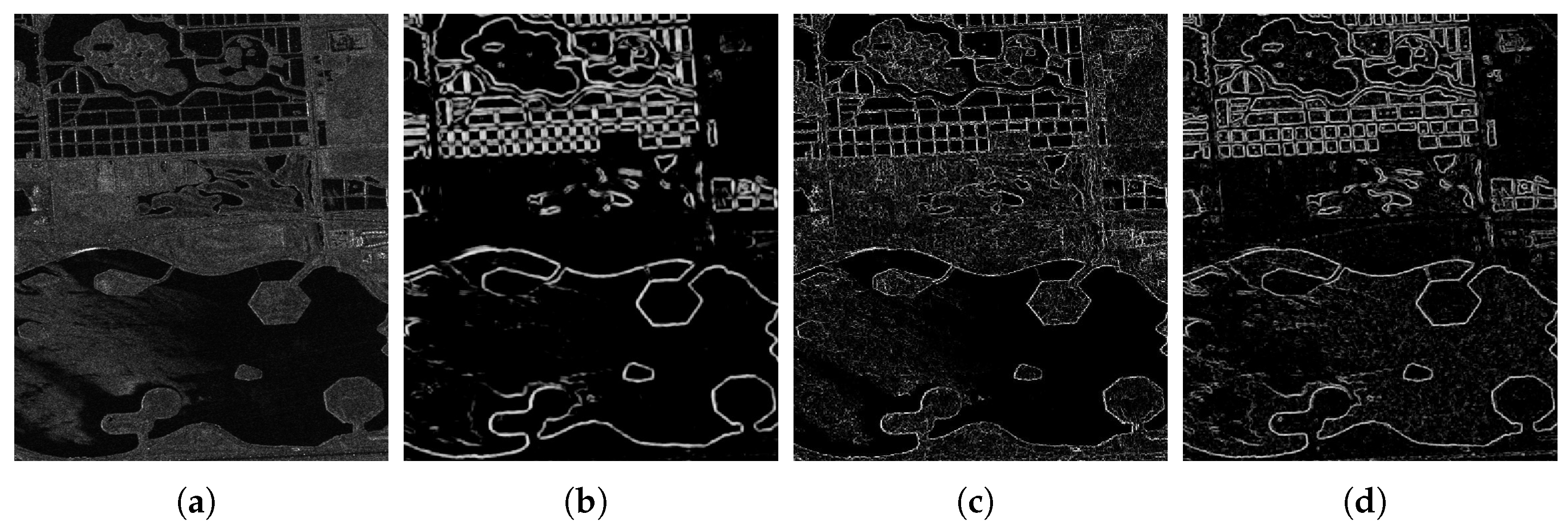
In order to compare the feature extraction capabilities of PC, SAR-PC, and GMPC, we tested them using real SAR images, as shown in Figure 4. For SAR images, the most important drawback of the traditional PC model is its sensitivity to multiplicative noise. Since the PC model assumes that the image noise is Gaussian white noise, it is difficult to cope with the strong scattering noise of SAR images. Both GMPC and SAR-PC are set to scale $s=3$ and the number of directions $n=6$, and the size of the GMF is kept the same as that of the Gabor filter used in SAR-PC. The rest of the parameters of SAR-PC follow the parameter settings suggested by the authors. In Figure 4b,d, GMPC has achieved better noise suppression capability.

2.2. SAR Modality Independent Neighborhood Fusion (SAR-MINF) Matching Algorithm

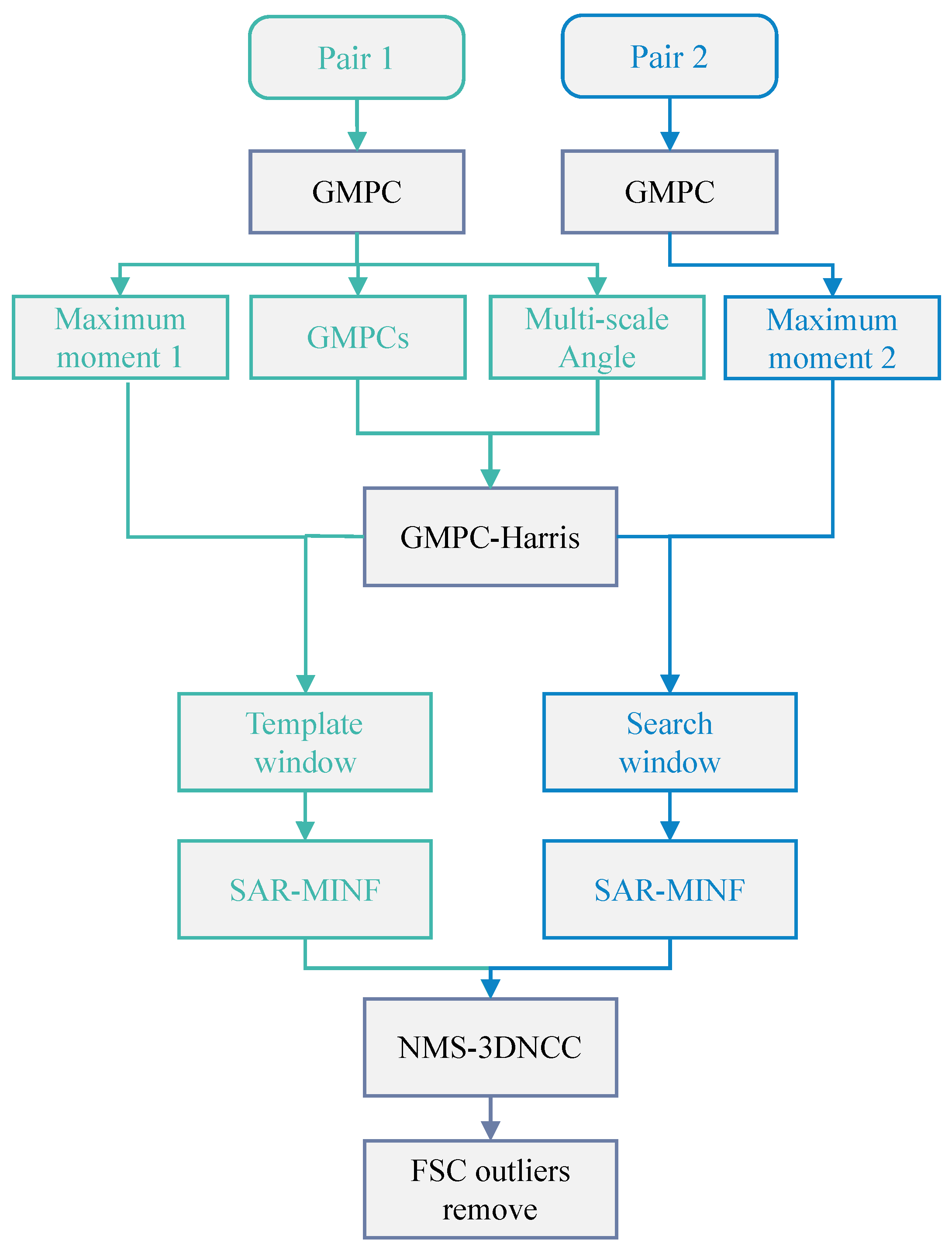
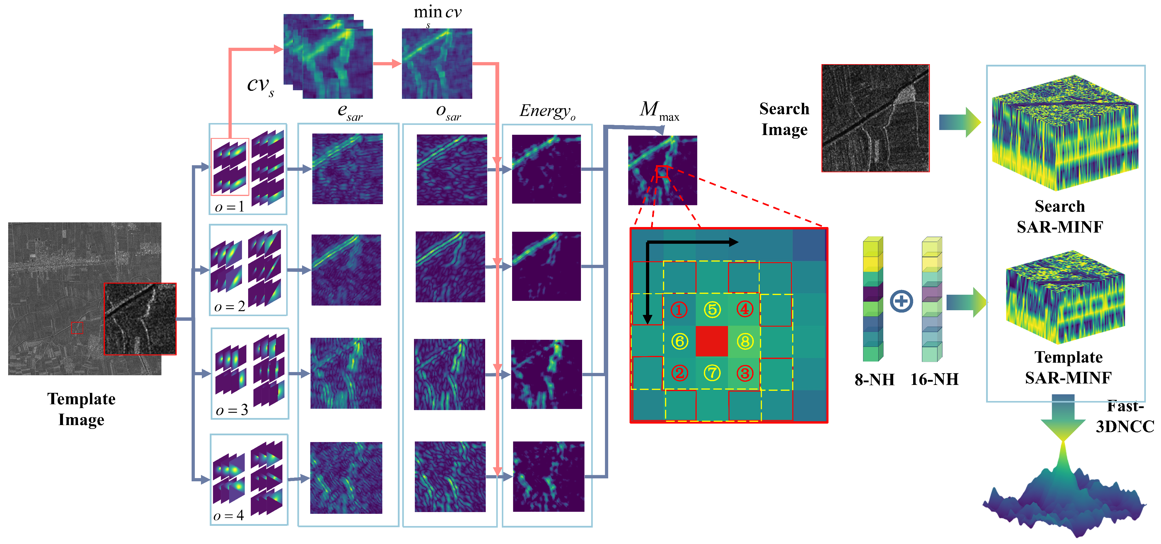
The complete matching flowchart is shown in the Figure 5. It follows the conventional matching process of this kind of method: keypoint detection, feature extraction, and template matching. For the feature matching step, to ensure efficiency and success rate of matching within the largest possible search window, we use the previously proposed NMS-3DNCC fast template matching algorithm [36]. Then, we introduce the keypoint detection and feature extraction parts in detail.

2.2.1. GMPC-Harris Keypoint Detection Based on Layover Perception

Due to the reliance on second-order derivatives of the Laplacian of Gaussian (LoG) and Hessian matrices for Harris keypoint extraction, the traditional Harris algorithm struggles to adapt to multiplicative noise. Based on the multiscale Harris function and GMPC, we propose a novel keypoint detection algorithm, GMPC-Harris. For the single-scale horizontal and vertical directions, $GMP{C}_s^x$ and $GMP{C}_s^y$ are defined as

$$\begin{array}{cc}\hfill GMP{C}_s^x& =⌊{\displaystyle \frac{{\sum }_o{W}_o(E_s^{\theta }-T_s)}{{\displaystyle \sum _s}{A}_s}}cos\theta ⌋,\theta =0\hfill \\ \hfill GMP{C}_s^y& =⌊{\displaystyle \frac{{\sum }_o{W}_o(E_s^{\theta }-T_s)}{{\displaystyle \sum _s}{A}_s}}sin\theta ⌋,\theta ={\displaystyle \frac{\pi }{2}}\hfill \end{array}$$

(14)

where $E_s^{\theta }$ represents the SAR energy function at scale s and angle $\theta$, and $T_s$ is the noise threshold corresponding to the $cv$ at scale s. From this, we can obtain GMPCs at different scales. The new multiscale GMPC-Harris matrix and the multiscale GMPC-Harris function, respectively, are obtained as follows:

$$\begin{array}{cc}\hfill & C_{MH}(x,y,s)={\mathcal{G}}_{\sqrt{2}·s}\ast \hfill \\ \hfill & \left[\begin{array}{cc}{\left(GMP{C}_s^x\right)}^2& \left(GMP{C}_s^x\right)·\left(GMP{C}_s^y\right)\\ \left(GMP{C}_s^x\right)·\left(GMP{C}_s^y\right)& {\left(GMP{C}_s^y\right)}^2\end{array}\right]\hfill \\ \hfill & R_{MH}(x,y,s)=det\left(C_{MH}(x,y,s)\right)-d·\mathrm{tr}\left(C_{MH}(x,y,s)\right)\hfill \end{array}$$

(15)

here, s denotes the current scale, and ${\mathcal{G}}_{\sqrt{2}·s}$ represents the Gaussian function at the current scale, with the scale parameter $\sigma$ of the Gamma filter as the standard deviation. d is an arbitrary parameter.

The angles of GMPC at different scales are defined as

$$Angl{e}_s=arctan\left({\displaystyle \frac{GMP{C}_s^y}{GMP{C}_s^x}}\right)$$

(16)

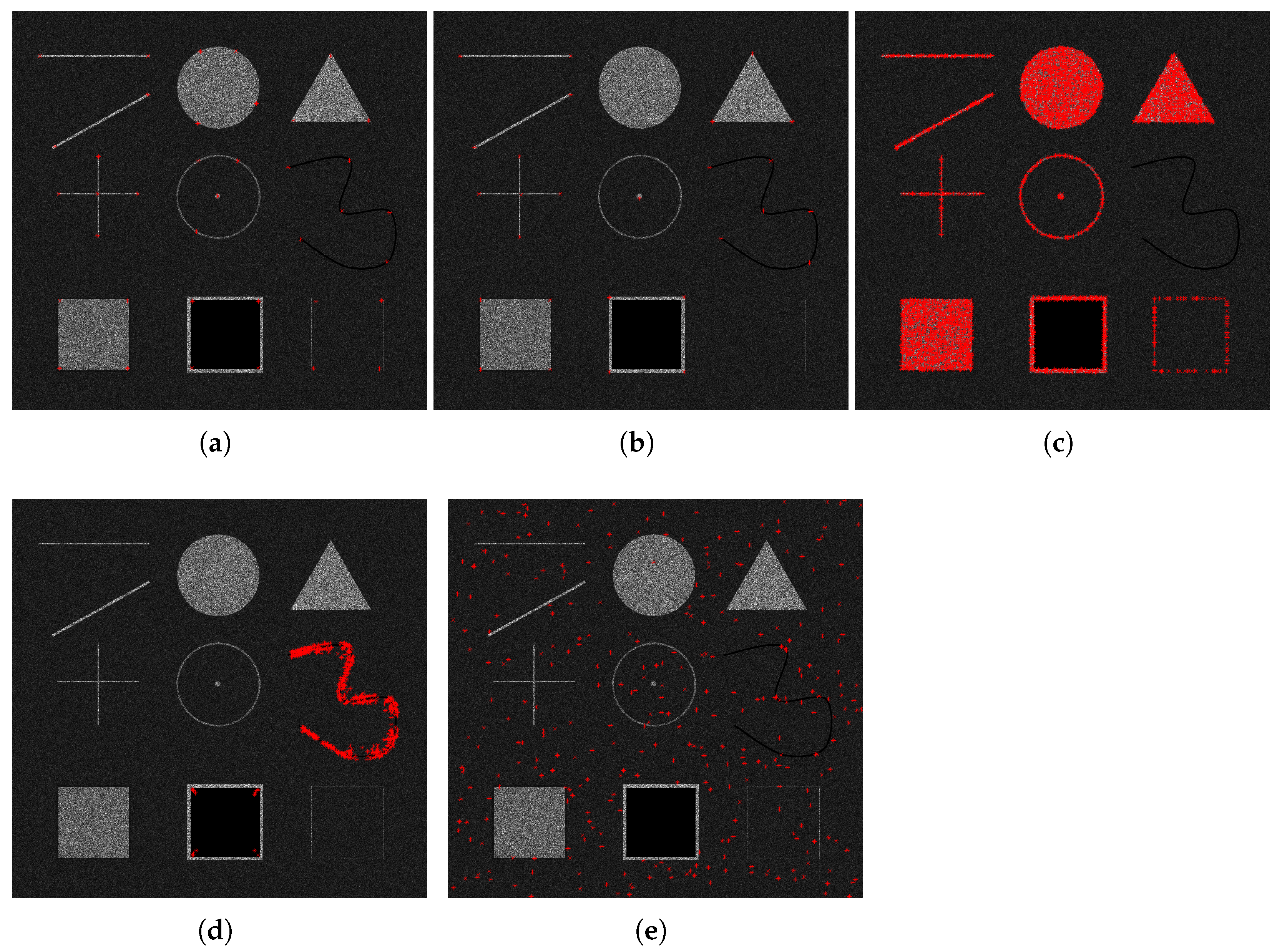
The process of identifying keypoints involves selecting local extrema at each scale space. These extrema are used as keypoint candidates, and their sub-pixel precision is refined by bilinear interpolation. To eliminate edges and low-contrast points, a threshold $d_{SH}$ is applied, allowing us to obtain the positions of the extrema and their response magnitudes. Non-maximum suppression is then performed based on the response values, ultimately identifying the keypoints with the strongest local responses. Figure 6 compares the effectiveness of different keypoint extraction methods on a simulated SAR image in Figure 3a. We use consistent parameter settings in both GMPC-Harris and SAR-Harris. Both methods exhibit superior keypoint distribution compared with other common algorithms. Notably, GMPC-Harris can detect subtle line features in the lower right of the image that SAR-Harris missed. Other algorithms, such as Harris, SURF, and FAST, struggled with noisy images and had difficulty detecting features.

Figure 7a showcases the actual image of a layover area. The fake texture facilitates the easier detection of keypoints. However, the textures in this area are considered invalid and can significantly impair matching accuracy and success rate. As depicted in Figure 7b, a layover or topographic displacement occurs when the radar beam reaches the top of a slope, point B, more quickly than it reaches the bottom, point A. This results in the reverse order of recording topographic features, with point b recorded before point a. The radar’s depression angle, local incidence angle, and ground point slope all influence layover. The impact of layover areas is more pronounced in ascending and descending orbits and mountainous regions. Hence, a method to identify and exclude these layover areas is necessary to enhance the overall quality of image matching.

As shown in Figure 7b, the identification of layover areas is fundamentally a geometric issue. In theory, we can approximate the satellite’s incidence angle and the local incidence angle by Digital Elevation Model (DEM) and the Rigorous SAR Positioning (RD) Model to identify the layover areas [37,38,39]. However, employing geometric models would necessitate the introduction of new parameter files, and the high computational complexity of the RD model would significantly reduce efficiency. Additionally, identifying layover areas for keypoint detection could lead to substantial redundant computations, making this approach impractical for SAR matching application. Therefore, a simpler and more effective method is needed to determine whether keypoints are located within layover areas.

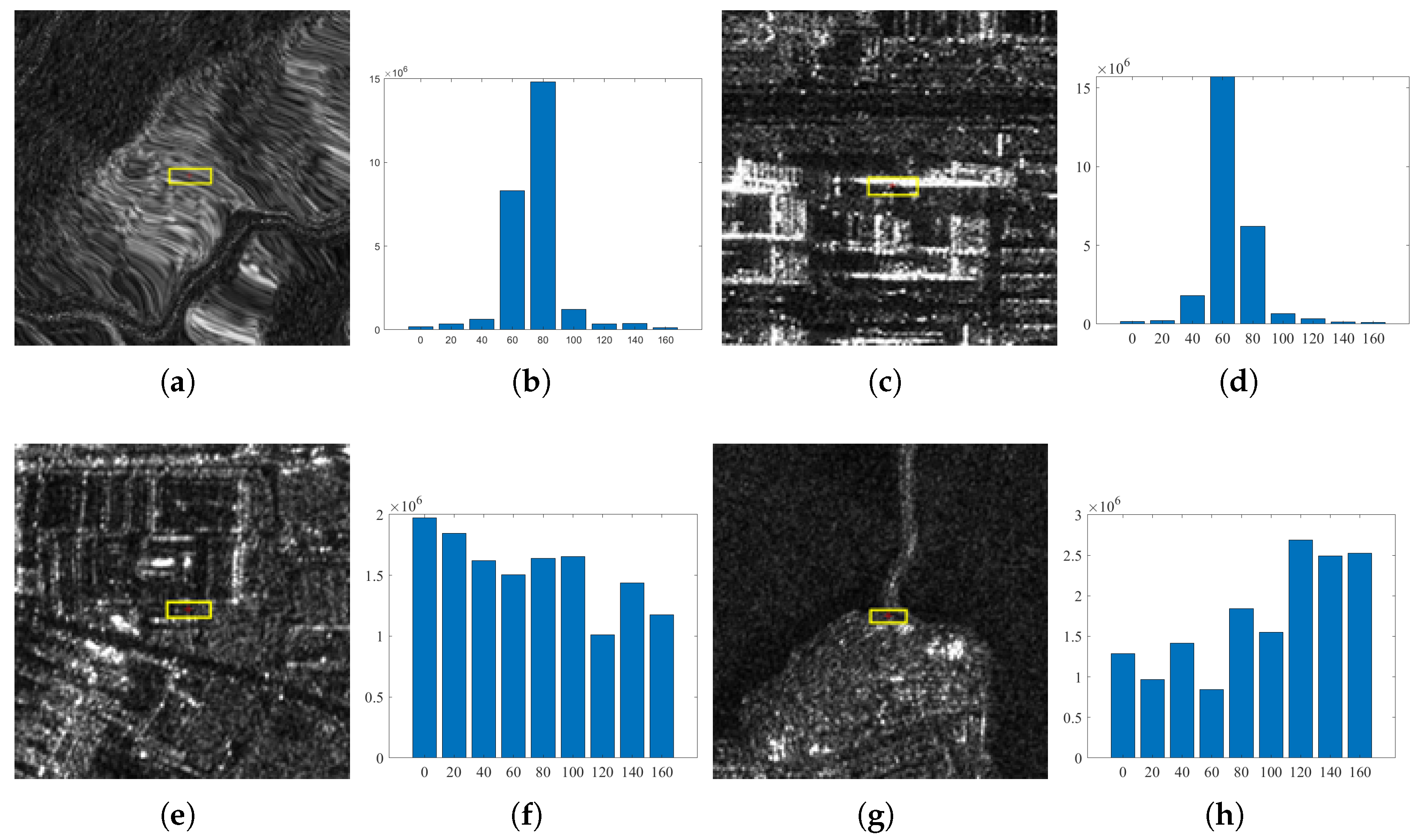
Observing layover areas, their textures typically exhibit strong directionality. Therefore, a layover area awareness method based on GMPC orientation histograms is proposed here to mitigate the impact of layovers on keypoint extraction. As shown in Figure 8, for a keypoint p, the first step is to construct its layover feature region. Since layover orientations generally occur along the range direction of SAR images, a rectangular template with $r_x>r_y$ is chosen to define this feature region. Given that excessively large R values not only reduce feature directionality but also increase computational complexity, we recommend to set $r_x=15,r_y=5$. The horizontal and vertical GMPCs $GMP{C}_s^x$ and $GMP{C}_s^y$ at different scales within the feature region can be obtained by Equation (14). The angle map $Angl{e}_s$ can be obtained from Equation (16), where the smallest scale is chosen as its angle map. Define the direction intervals $n_{bins}$ and assign gradient magnitudes to the corresponding $n_{bin}$, then, the GMPC orientation histogram $H_{GMPC}$ can be counted.

Compared with regular areas, layover areas exhibit a much stronger directionality, typically manifesting along the range direction. So it is possible to achieve layover area awareness for keypoints by this characteristic. Thus, by sorting all $n_{bins}$ in $H_{GMPC}$, and comparing the maximum value interval with the average of the other intervals, a region is identified as a layover area if it exceeds the threshold $t_f$:

$${\displaystyle \frac{V_{maxbin}}{V_{meanbins}}}>t_f$$

(17)

where $n_{bins}$ is usually set to 6, and $t_f$ can be set to 3. We test the images of mountainous areas and urban buildings, as shown in Figure 9. The yellow points represent the points in the layover areas, and the red points are the GMPC-Harris feature points that were ultimately detected. It can be observed that the proposed algorithm effectively eliminates pseudo-feature points in the layover areas while preserving the genuine feature points in the non-layover areas.

2.2.2. Feature Extraction Based on SAR-MINF

The GMPC is extended to use phase congruency in angular space to construct the maximum moments for edge feature detection:

$$GMPC=\sum _{o}GMPC\left({\theta }_o\right)$$

(18)

Then, the maximum moment of the GMPC is recorded as follows:

$$M_{max}={\displaystyle \frac{1}{2}}\left(a+c+\sqrt{b^2+{(a-c)}^2}\right)$$

(19)

where,

$$a=\sum {(GMPC\left(\theta \right)cos\left(\theta \right))}^2$$

(20)

$$b=2\sum \left(GMPC\right(\theta )cos(\theta \left)\right)·\left(GMPC\right(\theta )sin(\theta \left)\right)$$

(21)

$$c=\sum {(GMPC\left(\theta \right)sin\left(\theta \right))}^2$$

(22)

Based on the GMPC maximum moments, we propose the SAR Modality Independent Neighborhood Fusion (SAR-MINF) descriptor by integrating the Modality Independent Neighborhood Descriptor (MIND) [40]. The MIND descriptor leverages the concept of image self-similarity, extracting unique structures within a local neighborhood based on the similarity of image patches. The MIND is defined as follows:

$$MIND(I,\overrightarrow{x},\overrightarrow{r})={\displaystyle \frac{1}{n}}exp\left(-{\displaystyle \frac{Dp(I,\overrightarrow{x},\overrightarrow{x}+\overrightarrow{r})}{V(I,\overrightarrow{x})}}\right),\overrightarrow{r}\in \mathbb{R}$$

(23)

where n is a normalizing constant, $\mathbb{R}$ is the set of all pixels (defined by relative shifts from x) involved in the search space, $D_p$ refers to the distance between the patch centered at point x and the patch centered at point $x+r$, which is the squared difference between the two patches:

$$D_p\left(I,\overrightarrow{x},\overrightarrow{x}+\overrightarrow{r}\right)=\sum _{\overrightarrow{p}\in P}{\left(I\left(\overrightarrow{x}+\overrightarrow{p}\right)-I(\overrightarrow{x}+\overrightarrow{r}+\overrightarrow{p})\right)}^2$$

(24)

$V(I,x)$ is the $D_p(I,\overrightarrow{x},\overrightarrow{x}+\overrightarrow{r})$ summed average of the points in the neighborhood search space of the point x in the image. Mattias P. Heinrich et al. [40] provided the neighborhood space for 2D-MIND, which includes common configurations like the four-neighborhood and eight-neighborhood. Feature descriptors such as GLOH [41] and DAISY [42] have demonstrated the advantages of circular sampling methods. Consequently, we have redefined the neighborhood sampling space for SAR-MINF, which is similar to GLOH and DAISY, as illustrated in Figure 10a. For a pixel $(x_0,y_0)$ within the region, we initially construct an 8-NH MIND descriptor for its eight-neighborhood. Additionally, to enhance the descriptor’s robustness, we construct a 16-NH MIND descriptor for the adjacent pixels in the four-neighborhood (indicated by the yellow dashed lines in Figure 10c) and the D-neighborhood (indicated by the red solid lines in Figure 10c). The descriptor is weighted by L2 normalization based on the distance to the central pixel, and then merged with the 8-NH MIND for corresponding pixels to obtain an eight-dimensional descriptor for the central pixel. Finally, a Gaussian kernel with ${\mathcal{G}}_{s=5,\sigma =1}$ is convolved with the Z-axis to obtain the SAR-MINF descriptor for pixel $(x_0,y_0)$, where convolution aims to further enhance resistance to noise and local deformations. By computing the descriptor for each pixel within the region, we achieve a dense representation of the SAR-MINF feature descriptors for the area.

SAR-MINF is constructed as follows:

• For a pixel $(x_0,y_0)$ within a region, an 8-NH MIND descriptor is initially constructed for its eight-neighborhood to capture local structure;
• To enhance the robustness of the descriptor, a 16-NH MIND descriptor is constructed for the adjacent pixels in its four-neighborhood (indicated by the yellow dashed lines in Figure 10c) and the D-neighborhood (indicated by the red solid lines in Figure 10c);
• The descriptors are weighted by L2 normalization based on their distance to the central pixel and then fused with the 8-NH MIND to form an eight-dimensional descriptor for the central pixel;
• To further improve resilience against noise and local deformations, the SAR-MINF descriptor for pixel $(x_0,y_0)$ is obtained by convolving the descriptor with a Gaussian kernel $G_{s=5,\sigma =1}$ along the Z-axis;
• The dense representation of the SAR-MINF feature descriptors for the region is achieved by aggregating the descriptors for each pixel within the area.

The complete construction process of SAR-MINF is shown in Figure 11. To ensure both matching efficiency and success rate under as large a search window as possible, we adopted the Fast-3DNCC matching strategy proposed in our previous research [36].

2.3. Large-Scale Tie Point Automatic Extraction Method

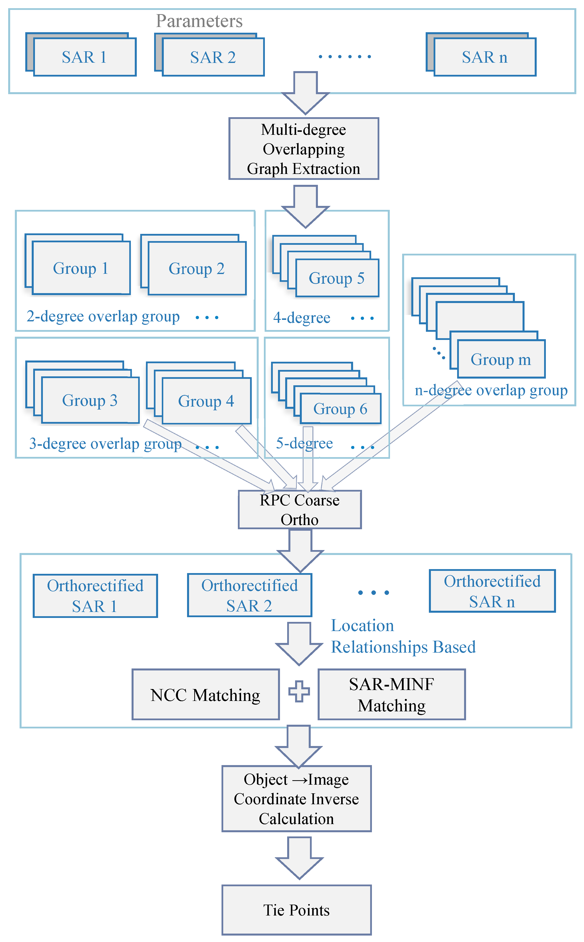
For large-scale tie point extraction, there is often a need to extract tie points between multiple images sharing common overlapping regions. Most tie point extraction methods currently available concentrate on matching between two images and then evaluating the overlap during the application process. This approach is similar to random events and can often lead to a shortage of tie points in areas where there is a high amount of overlap. To address this issue, we have refined the matching process for tie points, as illustrated in Figure 12.

2.3.1. Graph-Based Extraction of Multidegree Overlapping Regions

A graph $G=(V,E)$ is a set of connectivity relations consisting of nodes and edges, where nodes are the basic elements of the graph, usually denoted by V, and edges denote line segments connecting two nodes in the graph, usually denoted by E.

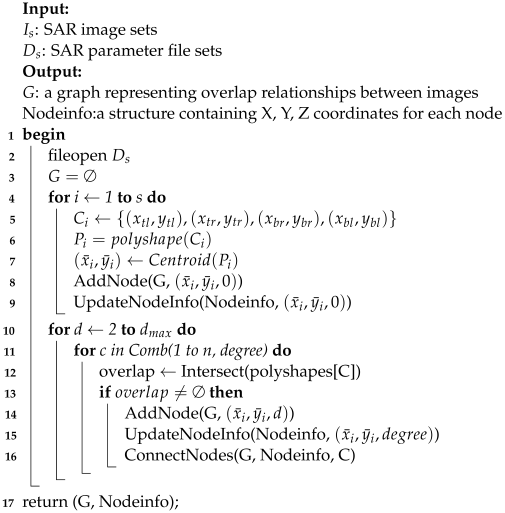
In this section, a multilevel graph structure is defined to represent the spatial relationships that exist between mutiple SAR images. Each SAR image is considered a node V in the graph and placed on the first level of the multilevel graph. The overlapping regions are represented by edges E, where an edge signifies an overlapping relationship between two nodes $(V_i,V_j)$. For image nodes with overlapping relationships, the overlapping regions will be added as a new overlapping node to a new level of the graph. To extract the overlapping regions and add them to the graph as nodes, a layer-by-layer scanning strategy is used here. For each potential overlap combination, the presence of an overlapping region is determined by calculating the intersection of polygons. If a non-empty overlap region is found, it is added as a new node to the graph, and edges are used to connect it to the original image nodes or lower-level overlap nodes that comprise the overlap region. Additionally, each overlap node is assigned an overlap degree label, which not only marks the coordinate information and the number of images involved in the overlap region but also indicates the level of the overlap in the graph. As the degree of overlap increases, highly overlapping nodes are placed at higher levels of the graph. The pseudocode for the algorithm is provided in Algorithm 1.

Algorithm 1: Algorithm of multidegree overlapping graph extraction.

The process of graph-based SAR multidegree overlapping regions extraction is as follows:

• Input Image and Parameter Files: The input SAR images here is Level 1 products, so each data package contains the SAR image data file $I_s$ and the SAR parameter data file $D_s$.
• Graph structure initialization: for each image $D_i\in D_s$, its quadrangle coordinates $C_i$ are obtained and polygonized to $P_i$. The centroid of each polygon ${\overline{x}}_i,{\overline{y}}_i$ is used as the position of the image nodes in graph G, and the Node and NodeInfo are initialized with level 0, to denote that they represent separate images instead of overlapping regions.
• Construction of overlapping region nodes: the algorithm further examines all possible combinations from two to n images to identify and construct overlapping region nodes. For each combination C, the algorithm computes the intersection of the polygons in the combination. If this intersection is non-empty, it indicates the existence of an overlapping region. The geometric centroid of the overlap area is used as the position for the new node. Subsequently, Node and NodeInfo are updated, with the level d, which signifies the degree of overlap.
• Nodes Connections: Each overlap region node needs to be connected to the image nodes or other overlap region nodes that make up that overlap region.
• Output: The output of the algorithm is the graph G, which accurately represents the muiltdegree overlapping relationships between the input SAR images. Additionally, the output includes the nodeInfo structure, which contains detailed information about each node within the graph.

2.3.2. Fusion Matching Method Based on Location Relationships

For the extraction of large-scale tie points from multiple SAR images, the positional relationships of SAR images are complex. However, the most common scenarios involve standard-width images derived from the same data segment through logical scene division, or data from the same orbit and same side-looking direction. For such images, the characteristics of the overlapping regions can remain essentially consistent or even completely identical, and the NCC algorithm is particularly suitable for the matching of these kinds of images due to its efficiency and stability. However, for images with significant differences, such as different orbits or side-looking directions, this consistency no longer exists, and traditional matching algorithms often struggle to deal with such complexity. In these situations, the SAR-MINF algorithm demonstrates its advantages, which can effectively deal with the matching problem in these complex cases and realize higher quality matching results. Therefore, we propose a fusion matching method based on the positional relationship of SAR images, which adopts different matching algorithms for image groups with different positional categories.

For the set of images within an overlapping group, a reference image must first be selected, with the remaining images serving as those to be matched. In the multidegree overlap graph, the node labels store the range of the overlap areas for each overlapping group. Based on this range, an external rectangular bounding box is delineated. Using the six coefficients of the reference image, all coarse orthorectified SAR images in the overlap group can be reprojected and cropped, thus obtaining matching images that are roughly aligned in both the image and object spaces, to complete the matching task for multiple degrees of overlap. The fusion matching method based on positional relationship is used to match each group of images, and the matched points are finally outputted as tie points after the Fast Sample Consensus (FSC) algorithm [43] of affine transform model, and then the final output is the object-to-image computation by the RPC model. This method, which integrates various algorithms and models, not only fully leverages their respective advantages but also effectively compensates for the shortcomings of each algorithm, providing an efficient and precise matching solution for SAR images under complex matching conditions.

3. Results and Discussion

To evaluate the proposed matching algorithm and tie point extraction method, this section conducts experiments on both. In the SAR-MINF matching experiment, SAR-MINF is first compared with various SAR image matching algorithms, including the traditional NCC algorithm, the SAR-PC algorithm based on regional feature matching [44], and feature-based algorithms such as SAR-SIFT [21], RIFT [45], and KAZE-SAR [22]. In the experiment on large-scale automatic tie point extraction, two sets of real SAR image experimental data are designed, and the results of the multidegree overlapping graph and tie point extraction are statistically analyzed.

3.1. SAR-MINF Matching Experiment

3.1.1. Data Sets and Parameter Settings

In order to cover SAR images with different imaging conditions as much as possible, eight groups of SAR image data were used here, such as in

Table 1. Information of the Test Images.

Pair	Sensor	Resolution	Band	Polarization	Orbit	Size	Region
A	ALOS2	2.5 m	L	HH	DEC	$1900\times 1900$	Urban
	GF3	3 m	C	DH	ASC
B	GF3	10 m	C	HH	DEC	$1239\times 1296$	Urban
	Sentinal-1A	10 m	C	VV	ASC
C	LT-1	3 m	L	HH	DEC	$2963\times 2963$	Urban, Mountain
	GF3	10 m	C	VV	ASC
D	GF3	10 m	C	HH	ASC	$2460\times 2460$	Airport
	GF3	10 m	C	HV	ASC
E	GF3	5 m	C	DH	DEC	$3287\times 2561$	Suburbs, Paddy
	GF3	3 m	C	DH	ASC
F	GF3	3 m	C	DH	ASC	$2133\times 1800$	Urban, Mountain
	GF3	3 m	C	DH	DEC
G	LT-1	3 m	L	HH	ASC	$1401\times 1401$	Urban
	GF3	3 m	C	VV	DEC
H	UMBRA	0.5 m	X	VV	ASC	$1953\times 1976$	Airport Terminal
	UMBRA	0.5 m	X	VV	ASC

and Figure 13, which cover different sensors, resolutions, wavebands, polarization modes, orbital orientations, and feature coverage scenes. Pair A includes images with differences in band and orbital direction. Due to the ALOS2 satellite being an L-band, urban scene interference is severe, making the noise more complex. Pair B consists of images from the same band and resolution but different sensors, with polarization and orbital direction variations. Pair C contains images with significant resolution, band, and polarization differences. Besides, it covers challenging matching scenes like mountainous areas. Pair D includes images with different polarization directions, which are relatively easier to match. Pair E to G all contain images from different orbital directions, with Pair E having differences in resolution, Pair F covering mountainous scenes, and Pair G showing differences in band and polarization mode. Pair H consists of public data from the UMBRA satellite [46], with a resolution of 0.5 m, classified as Very High Resolution (VHR) images, which are more challenging to match. All data have been orthorectified with RPC and cropped. The sixth pair employed DEM for orthorectification, which might result in distortion of the terrain features, while the other images were orthorectified using an average elevation.

The filter template radius determines the template size of the filter, thereby affecting the sharpness of the extracted features. A too small radii reduces the filter’s ability to resist noise, whereas an excessively large radii compromises feature localization accuracy. Similarly, the scale parameter influences the utilization of multiscale information. However, like the filter template radius, too few scales result in features being overly affected by noise, while too many scales reduce the feature localization capability. The initial scale parameter corresponds to the smallest scale of the filter, and the scale parameters for other scales are determined by multiplying the initial scale with the scale ratio coefficient.

The experimental parameter settings were as follows: In the GMF, the filter template radius $r=15$, the shape parameter $k=1$, and the constant term $t=2$. The scale parameter ${\sigma }_1=2$, the scale ratio ${\sigma }_i/{\sigma }_{i-1}=1.8$, the number of scales $s=3$, and the number of directions $n=6$. For the proposed algorithm, NCC, and SAR-PC method, the sizes of the template window and search window depended on the experimental data. The proposed algorithm used the GMPC-Harris keypoint extraction with layover perception (LP), and its parameter settings followed those outlined previously. The keypoint extraction of SAR-PC and NCC did not use the LP function. The other three algorithms, SAR-SIFT, KAZE-SIFT, and RIFT, belong to feature-based matching algorithms, and all their parameters followed the recommended settings in the original papers. All algorithms employ the FSC algorithm to eliminate outliers with $RMSE<3$. The experiments were conducted on an i9-13900K @5.4GHz, 64GB RAM, and MATLAB 2023B environment.

3.1.2. Evaluation Criteria

• Number of Correct Matches (NCM): The number of correct matches after the outlier removal step.
• Correct Matching Rate (CMR):

  $$CMR={\displaystyle \frac{NCM}{N_{total}}}$$

  (25)
  $N_{total}$ is the number of keypoints, that is, the total number of points to be matched.
• Root Mean Squared Error (RMSE):

  $$RMSE=\sqrt{{\displaystyle \frac{1}{N}}\sum _{i=1}^N({({x^{\prime }}_i-x_i^{gt})}^2+{({y^{\prime }}_i-y_i^{gt})}^2)}$$

  (26)
  We selected 10–20 pairs of corresponding points manually as the ground truth, including the keypoints $(x_i,y_i)$ of the template image and the matched points $(x_i^{gt},y_i^{gt})$ of the search image. $({x^{\prime }}_i,{y^{\prime }}_i)=\mathbf{H}\times (x_i,y_i)$, $\mathbf{H}$ is the affine transformation matrix.

3.1.3. Results and Discussion

The comparison of the experimental results for the eight sets of data is displayed in

Table 2. Numbers of keypoints, NCM, CMR, RMSE, total time, and TPP of Different Descriptors.

Pair	Template Radius	Search Radius	Performance	SAR-MINF	SAR-MINF (Without LP)	NCC	SAR-PC	SAR-SIFT *	KAZE-SAR *	RIFT *
A	105	75	Keypoints	382	440	440	440	\	\	\
			NCM	295	327	47	258	5	3	116
			CMR	77.23%	74.32%	10.68%	58.64%	\	\	\
			RMSE	1.1274	1.1306	7.4491	1.5483	587.3138	1337.36	1.5794
B	65	35	Keypoints	209	278	278	278	\	\	\
			NCM	191	252	173	231	19	12	221
			CMR	91.39%	90.65%	62.23%	83.09%	\	\	\
			RMSE	1.6674	1.7491	2.6119	2.014	3.1713	7.5040	1.9173
C	65	35	Keypoints	781	931	931	931	\	\	\
			NCM	704	829	817	841	330	267	326
			CMR	90.14%	89.04%	87.76%	90.33%	\	\	\
			RMSE	0.7864	0.8232	0.9755	0.7967	1.1739	1.0559	1.0824
D	70	40	Keypoints	467	493	493	493	\	\	\
			NCM	426	446	413	426	222	414	369
			CMR	91.22%	90.47%	83.77%	86.41%	\	\	\
			RMSE	0.3189	0.3274	0.9182	0.4710	2.4707	0.3902	0.3498
E	60	35	Keypoints	747	1081	1081	1081	\	\	\
			NCM	677	924	907	928	366	217	202
			CMR	90.63%	85.48%	83.90%	85.58%	\	\	\
			RMSE	0.8973	0.8981	1.1818	1.1179	1.2343	0.9228	1.7696
F	55	15	Keypoints	239	276	276	276	\	\	\
			NCM	208	231	111	183	40	25	260
			CMR	87.03%	83.70%	40.22%	66.30%	\	\	\
			RMSE	0.8782	0.9574	2.2352	1.1126	2.0194	4.264	1.6853
G	65	35	Keypoints	352	388	388	388	\	\	\
			NCM	241	246	37	238	9	1	137
			CMR	68.47%	63.40%	9.54%	61.34%	\	\	\
			RMSE	0.6029	0.7298	7.7269	0.5596	38.6447	1218.50	2.0871
H	80	40	Keypoints	451	457	457	457	\	\	\
			NCM	225	230	169	172	24	64	110
			CMR	49.81%	50.33%	36.98%	37.64%	\	\	\
			RMSE	1.1357	1.077	2.4045	1.7218	99.7471	34.3372	3.817

* SAR-SIFT, KAZE-SAR, and RIFT belong to feature-based matching methods; therefore, the NCM and CMR are not counted. The optimal values in the table are in bold and the suboptimal values are in italics.

and Figure 14, where the optimal values are shown in bold.

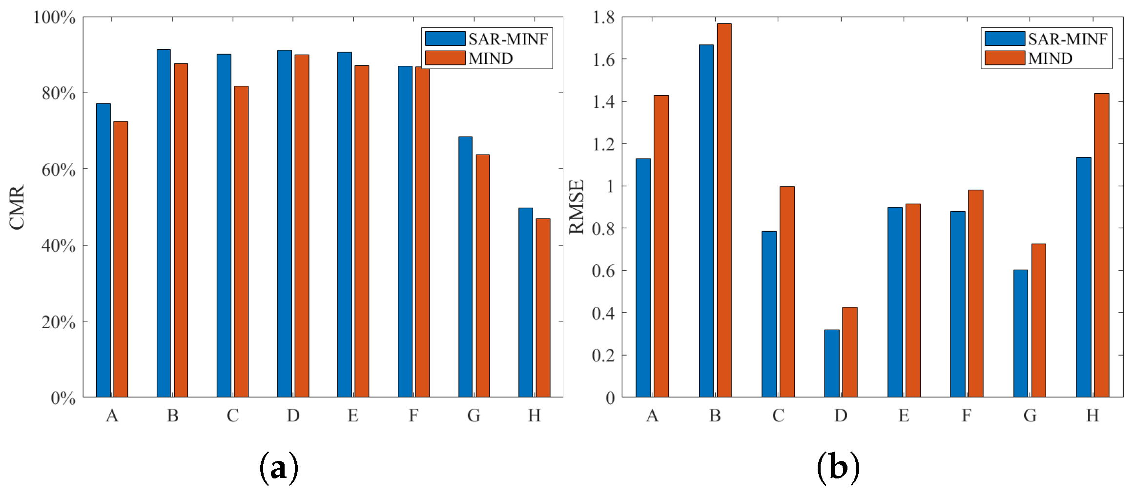
SAR-MINF exhibits better RMSE and CMR in most test data sets. Compared with SAR-MINF without LP, its CMR is ahead by 2.97% on average, and in the higher resolution ascending–descending orbit image pairs A, E, F, and G, it leads by an average of 6.00%. Except for pair H, its RMSE has also improved across the board; however, since the number of successfully matched points is already high, the increase in RMSE is not significant.

Compared with the commonly used NCC algorithm, the CMR of the proposed algorithm has an average lead of 182.30% for all data, while it is substantially ahead of the five pairs of images, A, B, F, G, and H, with an average lead of 287.76%; and the average lead in RMSE across all scenarios is 54.43%.

When compared with the SAR-PC algorithm, the proposed algorithm’s CMR leads by an average of 16.02% across all scenarios, although the SAR-PC algorithm does lead in CMR for pair C. The average lead in RMSE across all scenarios is 18.14%, with the SAR-PC algorithm leading in RMSE for pair G and performing similarly to the proposed algorithm in pairs C and D, which are standard scenarioss. However, SAR-PC’s performance is slightly inferior in more complex scenarios such as ascending–descending orbits and VHR, but it still leads the other algorithms.

SAR-SIFT, KAZE-SAR, and RIFT are all feature-based matching algorithms, and their CMRs are not strictly comparable with the previous three algorithms; among them, the SAR-SIFT algorithm fails to match in the pairs A, G, and H; the KAZE-SAR fails to match in the pairs A, B, G, and H; the performance of RIFT is the best among the three, while second only to SAR-PC; and the proposed algorithm improves the RMSE by 39.55% on average in all scenes compared with RIFT. However, we found that the results of the RIFT algorithm are random. For example, we conducted five consecutive RIFT matches on pair G and recorded the NCM and RMSE, as shown in Figure 15, and the RMSE can even vary up to approximately threefold. Therefore, the average of five consecutive experiments was taken as the final result. Additionally, the unstable performance of RIFT makes it challenging to apply in engineering applications.

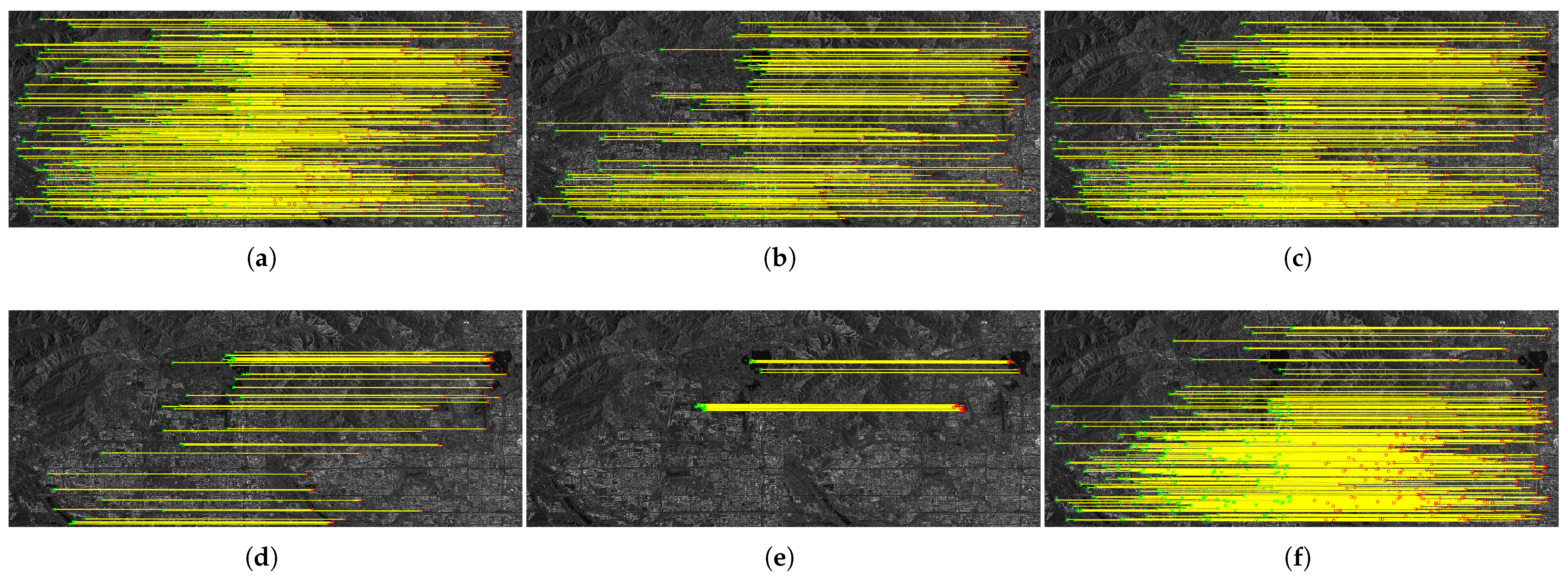
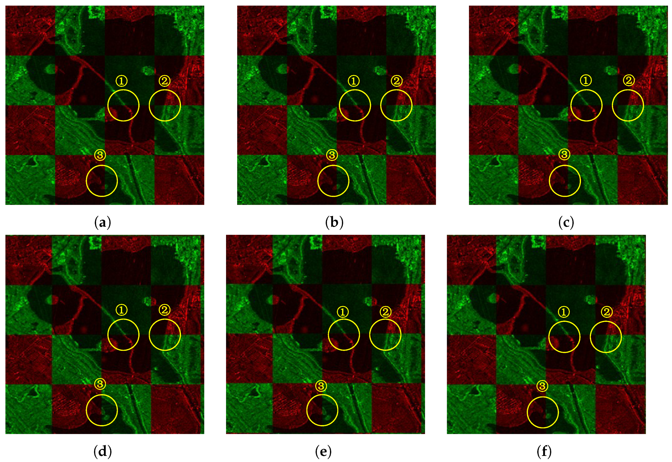
In order to visually compare the matching effect of different algorithms, we select the pair F that is successfully matched by each algorithm and give the matching result diagrams of different algorithms (Figure 16) and the enlarged checkboard mosaic sub-images (Figure 17). To clearly display the SAR images, the results are color-processed separately for the two images, with the red one representing the image to be matched and the green one representing the target image. In Figure 16, SAR-MINF has the most uniform distribution of matched points and successfully matches the feature points of the mountainous areas in the upper left part of the images, while the other algorithms do not.

In Figure 17, SAR-MINF achieves the best registration at ①–③; NCC exhibits a vertical axis offset at the shoreline in ① and ③; SAR-PC shows a horizontal axis offset at ①; SAR-SIFT has horizontal axis offsets at the shoreline in ① and the islet in ③; KAZE-SAR presents horizontal axis offsets at the shoreline in ① and ②, and islet in ③; and RIFT demonstrates horizontal axis offsets at the shoreline in ② and the islet in ③. These results are consistent with the data for pair F presented in Table 2.

In order to visualize the matching results of the proposed algorithm, the checkerboard mosaics of all the experimental images of the SAR-MINF algorithm and their enlarged sub-images are given below in Figure 18.

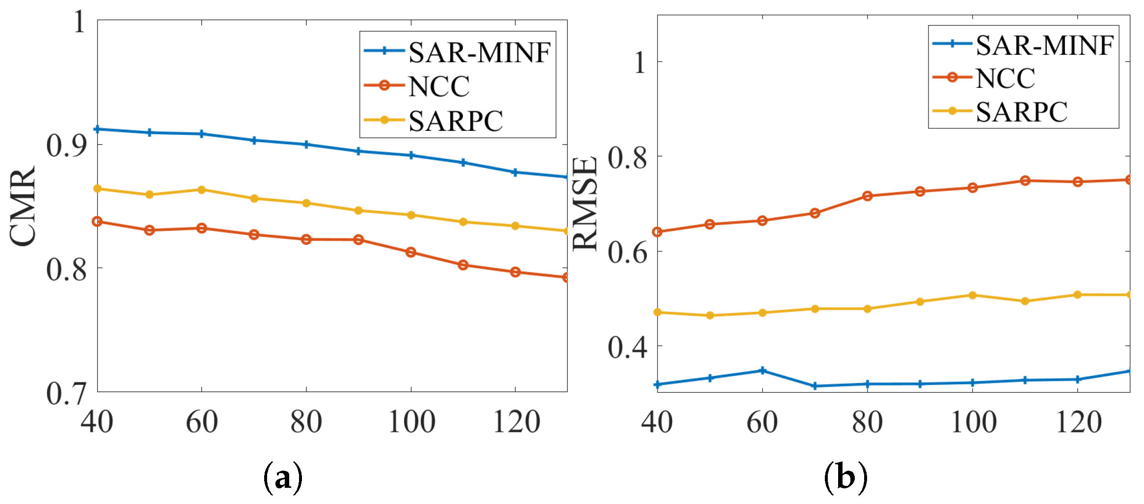
In practical applications such as tie point extraction, the performance of matching methods under large search radii is crucial. To evaluate the performance of the proposed method under different search radii, we conduct experiments on three area-based matching methods by pair D. The CMR and RMSE were recorded as shown in Figure 19. As the search window size increased, the CMR of all three algorithms decreased to some extent, with SAR-MINF consistently maintaining the highest CMR among the three algorithms. NCC’s RMSE increased to a certain degree, while the RMSE for SAR-MINF and SAR-PC algorithms remained relatively stable, demonstrating robustness to large search radii.

To evaluate the effectiveness of SAR-MINF neighborhood fusion, an ablation experiment was conducted. In this experiment, only the neighborhood feature was statistically analyzed using the feature sampling space of the MIND, without performing the feature fusion step. The CMR and RMSE were computed, as shown in Figure 20. Compared with the case without neighborhood fusion, the proposed algorithm achieved an average improvement of 4.81% in CMR and a reduction of 14.47% in RMSE.

The running efficiency statistics of different algorithms are shown in

Table 3. The comparison of algorithms efficiency.

Pair	SAR-MINF	NCC	SAR-PC	SAR-SIFT	KAZE-SAR	RIFT
B	15.65 s	5.06 s	14.15 s	98.48 s	20.97 s	6.10 s
C	47.35 s	15.23 s	44.98 s	708.86 s	363.53 s	20.71 s

, taking pairs B and C as examples. The computational complexity of the proposed algorithm is approximately 3.1 times that of NCC and about 1.1 times that of the SAR-PC algorithm, and its time to complete the matching is acceptable. Since NCC does not need to perform any feature extraction process, it has high computational efficiency, which is the reason why NCC is used in our proposed fusion matching method for tie point extraction. On the other hand, SAR-SIFT and KAZE-SAR, due to extracting a large number of feature points during the feature point extraction stage and their high feature dimensions, result in extremely high time complexity. The RIFT algorithm is more efficient, but due to its significant randomness, it needs to be run multiple times to achieve optimal matching, thus the actual algorithm time is higher.

In order to determine the impact of the LP strategy on the efficiency of the algorithm, we calculated the running time of the LP strategy. As shown in

Table 4. Impact of LP strategy on algorithm efficiency.

Pair	A	B	C	D	E	F	G	H
GMPC-Harris	2.851 s	1.458 s	7.375 s	4.855 s	7.384 s	3.105 s	1.822 s	2.976 s
GMPC-Harris+LP	2.97 s	1.535 s	7.587 s	4.983 s	7.615 s	3.209 s	1.931 s	3.105 s
LP	0.119 s	0.077 s	0.212 s	0.128 s	0.231 s	0.104 s	0.109 s	0.129 s

, It can be seen that the LP strategy has little impact on the efficiency of the algorithm, due to the fact that the histogram of directions is already obtained when computing the GMPC, and therefore, it is only necessary to compare them statistically without having to compute them again.

3.2. Tie Point Automatic Extraction Experiment

3.2.1. Data Sets and Parameter Settings

We selected two sets of SAR images to test the proposed large-scale automatic tie point extraction workflow, as shown in Figure 21. The first set contains eight SAR images of FSII mode from Gaofen-3(GF3), primarily covering the Shandong province. This set includes six ascending right-looking images and two descending right-looking images, and it features a significant difference in incidence angles. This set was designed to evaluate the algorithm’s ability to extract tie points under complex imaging conditions. The second set contains 34 SAR images of FSI mode from GF-3, covering a more comprehensive range, including Hebei, Shanxi, and parts of Beijing and Inner Mongolia. With a more extensive data volume and a more diverse range of geographic features, this set more closely represents the data distribution scenarios typically encountered in producing real surveying and mapping products. It was primarily used to test the stability of the proposed algorithm with a large volume of data. Specific information about the two data sets is provided in

Table 5. Information for the TPs test data.

Parameter	First Set of Images	Second Set of Images
Number of Images	8 scenes	34 scenes
Sensor	GF3	GF3
Imaging Mode	FSII	FSI
Nominal Resolution	10 m	5 m
Ortho Raster Resolution	3.4 m × 4.2 m	3.1 m × 3.8 m
Swath Width	About 110 km	About 50 km
Orbital Direction	2 descending and 6 ascending	All descending
Polarization Direction	HH	HH
Incidence Angle Difference	${22.53}^{°}\sim {34.78}^{°}$	${33.15}^{°}\sim {38.52}^{°}$
Slant Range Dimension	About $\mathrm{29,000}\times \mathrm{27,000}$	About $\mathrm{15,000}\times \mathrm{20,000}$
Terrain Features	Plains, cities, mountains, etc.	Mountains, cities, plains, etc.

.

We implemented the proposed algorithms with C++. Additionally, we developed an independent module for large-scale automatic tie point extraction. To achieve the intersection of polygons, we used the GEOS library [47]. Also, we used GDAL [48] for raster operations, including ortho, reprojection, and I/O. The core parts of the algorithms were mainly developed by OpenCV [49], Eigen [50], and FFTW [51] libraries. The experiments were conducted on a Windows 11 PC with an i9-13900K @5.4GHz processor, 64GB DDR5 memory, and 4TB PCIE4.0 SSD.

In the preprocessing step, the RPC model was used for ortho, with the resolution of the orthoimages being automatically calculated by the model. Contrast stretching of the SAR images was performed using a lower threshold of $1\%$ and an upper threshold of $99\%$. For the first set of images, the maximum degree of overlap was set to 5; and for the second set, it was set to 3. In the matching step, for the first set of images, the maximum number of keypoints for each overlapping group was limited to 300; and for the second set, due to the large number of images and the complexity of the overlapping relationships, the maximum number of keypoints for each overlapping group was set to 100. The parameter settings for the SAR-MINF feature part in this section remained consistent with the earlier sections; the template radius was set at 35, and the search radius was established at 150. The threshold for the ratio of the primary to secondary peak values was set at 0.6. Outliers were eliminated using an affine transformation model and the FSC algorithm, with $RMSE=3$.

3.2.2. Experimental Results and Discussion

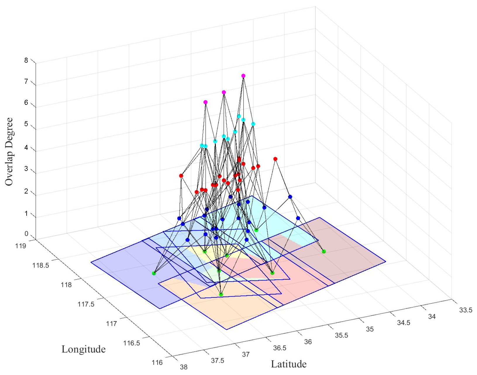
For the first set of images, their multidegree overlapping graph is shown in Figure 22. Nodes of different colors in the graph indicate overlapping groups with different degrees of overlap, and the lines between the nodes indicate that they have overlapping relationships. This group of images has regions with up to 6 degrees of overlap. However, due to the minimal area covered by the 6-degree overlap regions, the maximum degree of overlap for this set of images was set to 5.

The ground control points were extracted by the multisource remote sensing image matching algorithm proposed by us [36]. Subsequently, block adjustment based on the RD model was performed separately for each group of images. The relative accuracy of tie points was calculated and summarized, as shown in

Table 6. Experimental results for the TPs extraction.

Group	ID	2-Degree Overlapping TPs			Multiple-Degree Overlapping TPs			RMSE
		Total Points	<0.5 ps Points	Percentage	Total Points	<0.5 ps Points	Percentage
1	1	375	371	98.93%	176	164	93.17%	0.1998
	2	791	777	98.23%	318	313	98.42%	0.1774
	3	751	739	98.40%	143	141	98.60%	0.1739
	4	548	538	98.17%	175	172	98.28%	0.1774
	5	550	542	98.55%	121	119	98.35%	0.1762
	6	238	233	97.89%	113	106	93.80%	0.1914
	7	491	487	99.18%	137	133	97.08%	0.1780
	8	517	511	98.83%	124	117	94.35%	0.1776
2	Total	4992	4869	97.53%	1183	1148	97.04%	0.1702

. For the first group of images, the number of tie points for each scene was tallied, while for the second group, with its larger number of images, a total number of all tie points was collected.

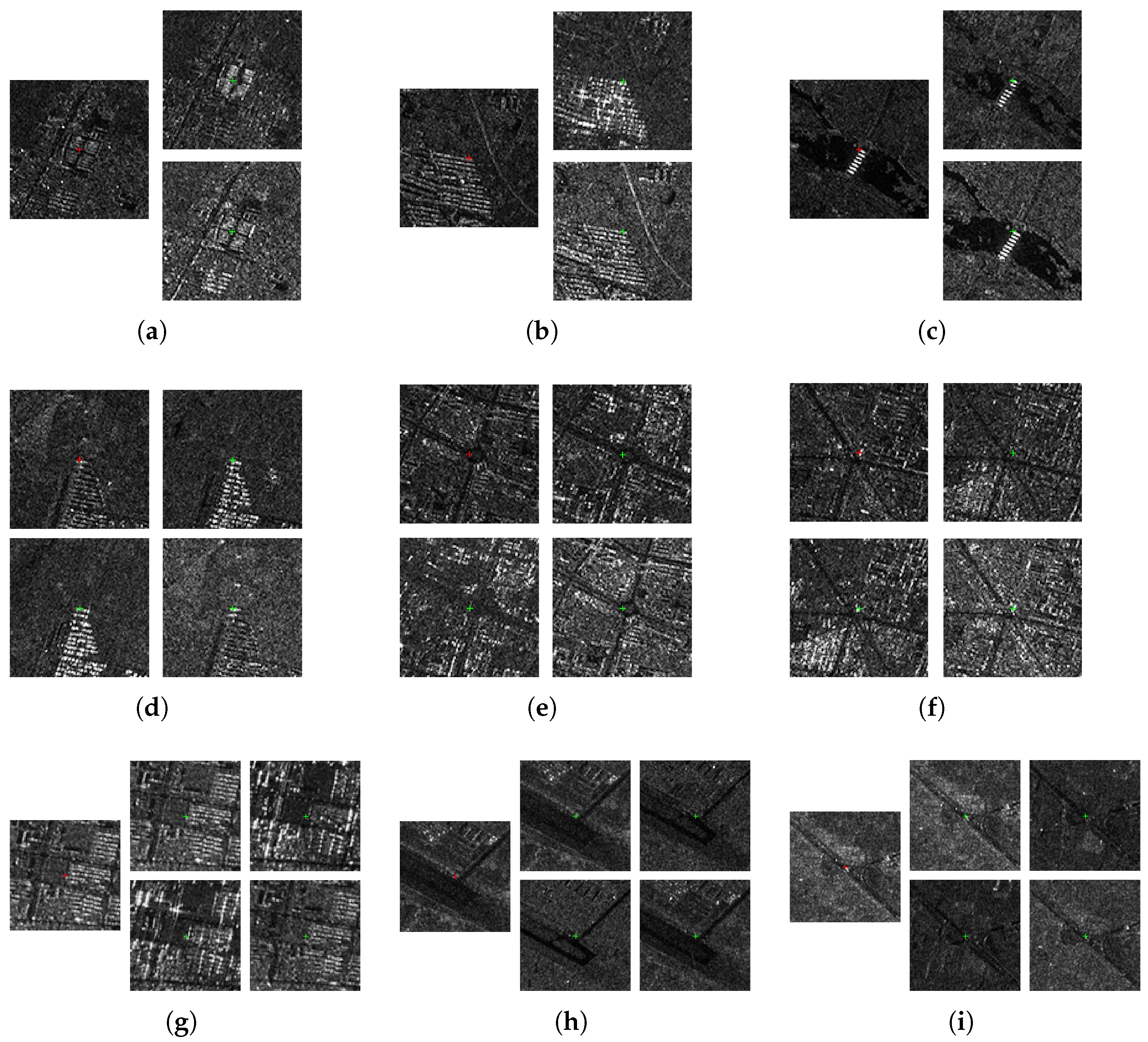
For the 2-degree tie points, the proposed algorithm demonstrated high matching precision, with the average proportion of tie points with $RMSE<0.5$ exceeding 98%. For multidegree tie points, the proportion of tie points with $RMSE<0.5$ decreased slightly due to the increased difficulty of matching, however, the average percentage was still over 95%. To intuitively understand the RMSE distribution of the two data sets, the histograms are illustrated as Figure 23. The majority of the tie points, both in 2-degree and multidegree overlapping areas, exhibited accuracies within sub-pixel error, which is sufficient for application needs. To visually demonstrate the matching results in multidegree overlapping areas, some of the 3- to 5-degree overlap tie points from the first data set are shown in Figure 24.

4. Conclusions

In this paper, to address the challenge of automatically extracting large-scale tie points of SAR images, we first introduced a novel SAR image matching algorithm SAR-MINF tailored to various imaging conditions. We established the novel matching algorithm for the extraction of SAR image tie points by benefiting the Gamma modulation phase congruency model, the layover perception algorithm, the GMPC-Harris feature point extraction algorithm, and the neighborhood feature fusion dense descriptor. Furthermore, a workflow for automatically extracting large-scale SAR tie points was built using a graph-based overlap degree extraction algorithm and a fusion matching method based on positional relationships. Experimental results show that SAR-MINF effectively improves the success rate and accuracy of SAR image matching under different imaging conditions. The proposed workflow for extracting large-scale tie points can achieve stable, high-precision extraction of multidegree overlapping tie points.

Although this study provides significant insights into SAR image matching under different imaging conditions and TPs automated extraction, the ability to extract TPs from SAR imagery in certain complex scenarios still requires improvement. Specifically, tie point extraction poses significant challenges in images with weak textures and rapid variations, such as those of deserts and large water bodies, as well as in images with substantial differences in incidence angles or pronounced terrain elevation changes. These challenges necessitate further in-depth research to achieve effective solutions.

References

1. Moreira, A.; Prats-Iraola, P.; Younis, M.; Krieger, G.; Hajnsek, I.; Papathanassiou, K.P. A tutorial on synthetic aperture radar. IEEE Geosci. Remote Sens. Mag. 2013, 1, 6–43. [Google Scholar] [CrossRef]
2. Li, Y.; Wu, J.; Mao, Q.; Xiao, H.; Meng, F.; Gao, W.; Zhu, Y. A Novel Two-Dimensional Autofocusing Algorithm for Real Airborne Stripmap Terahertz Synthetic Aperture Radar Imaging. IEEE Geosci. Remote Sens. Lett. 2023, 20, 4012405. [Google Scholar] [CrossRef]
3. Guo, L.; Wang, X.; Wang, Y.; Yue, M. A new approach of digital orthorectification map generation for GF3 satellite data. In Proceedings of the 2019 6th Asia-Pacific Conference on Synthetic Aperture Radar (APSAR), Xiamen, China, 26–29 November 2019; IEEE: Piscataway, NJ, USA, 2019; pp. 1–4. [Google Scholar]
4. Rignot, E.J.; Van Zyl, J.J. Change detection techniques for ERS-1 SAR data. IEEE Trans. Geosci. Remote Sens. 1993, 31, 896–906. [Google Scholar] [CrossRef]
5. Marin, C.; Bovolo, F.; Bruzzone, L. Building change detection in multitemporal very high resolution SAR images. IEEE Trans. Geosci. Remote Sens. 2014, 53, 2664–2682. [Google Scholar] [CrossRef]
6. Mao, Q.; Li, Y.; Zhu, Y. A hierarchical feature fusion and attention network for automatic ship detection from SAR images. IEEE J. Sel. Top. Appl. Earth Obs. Remote Sens. 2024, 17, 13981–13994. [Google Scholar] [CrossRef]
7. Chanussot, J.; Mauris, G.; Lambert, P. Fuzzy fusion techniques for linear features detection in multitemporal SAR images. IEEE Trans. Geosci. Remote Sens. 1999, 37, 1292–1305. [Google Scholar] [CrossRef]
8. Shakya, A.; Biswas, M.; Pal, M. Fusion and classification of multi-temporal SAR and optical imagery using convolutional neural network. Int. J. Image Data Fusion 2022, 13, 113–135. [Google Scholar] [CrossRef]
9. Wang, J.; Lv, X.; Huang, Z.; Fu, X. An Epipolar HS-NCC Flow Algorithm for DSM Generation Using GaoFen-3 Stereo SAR Images. Remote Sens. 2022, 15, 129. [Google Scholar] [CrossRef]
10. Kennedy, R.; Cohen, W. Automated designation of tie-points for image-to-image coregistration. Int. J. Remote Sens. 2003, 24, 3467–3490. [Google Scholar] [CrossRef]
11. Liu, L.; Wang, Y.; Wang, Y. SIFT based automatic tie-point extraction for multitemporal SAR images. In Proceedings of the 2008 International Workshop on Education Technology and Training & 2008 International Workshop on Geoscience and Remote Sensing, Washington, DC, USA, 21–22 December 2008; IEEE: Piscataway, NJ, USA, 2008; Volume 1, pp. 499–503. [Google Scholar]
12. Zou, W.; Chen, L. Determination of optimum tie point interval for SAR image coregistration by decomposing autocorrelation coefficient. IEEE Trans. Geosci. Remote Sens. 2019, 57, 5067–5084. [Google Scholar] [CrossRef]
13. Shi, W.; Su, F.; Wang, R.; Fan, J. A visual circle based image registration algorithm for optical and SAR imagery. In Proceedings of the 2012 IEEE International Geoscience and Remote Sensing Symposium, Munich, Germany, 22–27 July 2012; IEEE: Piscataway, NJ, USA, 2012; pp. 2109–2112. [Google Scholar]
14. Suri, S.; Reinartz, P. Mutual-information-based registration of TerraSAR-X and Ikonos imagery in urban areas. IEEE Trans. Geosci. Remote Sens. 2009, 48, 939–949. [Google Scholar] [CrossRef]
15. Kuglin, C.D. The phase correlation image alignment methed. In Proceedings of the International Conference Cybernetics Society, San Francisco, CA, USA, 23–25 September 1975. [Google Scholar]
16. Yu, L.; Zhang, D.; Holden, E.J. A fast and fully automatic registration approach based on point features for multi-source remote-sensing images. Comput. Geosci. 2008, 34, 838–848. [Google Scholar] [CrossRef]
17. Shi, X.; Jiang, J. Automatic registration method for optical remote sensing images with large background variations using line segments. Remote Sens. 2016, 8, 426. [Google Scholar] [CrossRef]
18. Ying, X.; Yan, Z. Sar Image Registration Using a New Approach Based on the Region Feature. In Proceedings of the Foundations of Intelligent Systems: Proceedings of the Eighth International Conference on Intelligent Systems and Knowledge Engineering (ISKE 2013), Shenzhen, China, 20–23 November 2013; Springer: Berlin/Heidelberg, Germany, 2014; pp. 603–613. [Google Scholar]
19. Lowe, D.G. Distinctive image features from scale-invariant keypoints. Int. J. Comput. Vis. 2004, 60, 91–110. [Google Scholar] [CrossRef]
20. Wang, S.; You, H.; Fu, K. BFSIFT: A novel method to find feature matches for SAR image registration. IEEE Geosci. Remote Sens. Lett. 2011, 9, 649–653. [Google Scholar] [CrossRef]
21. Dellinger, F.; Delon, J.; Gousseau, Y.; Michel, J.; Tupin, F. SAR-SIFT: A SIFT-like algorithm for SAR images. IEEE Trans. Geosci. Remote Sens. 2014, 53, 453–466. [Google Scholar] [CrossRef]
22. Pourfard, M.; Hosseinian, T.; Saeidi, R.; Motamedi, S.A.; Abdollahifard, M.J.; Mansoori, R.; Safabakhsh, R. KAZE-SAR: SAR image registration using KAZE detector and modified SURF descriptor for tackling speckle noise. IEEE Trans. Geosci. Remote Sens. 2021, 60, 1–12. [Google Scholar] [CrossRef]
23. Ye, Y.; Bruzzone, L.; Shan, J.; Bovolo, F.; Zhu, Q. Fast and robust matching for multimodal remote sensing image registration. IEEE Trans. Geosci. Remote Sens. 2019, 57, 9059–9070. [Google Scholar] [CrossRef]
24. Xiang, Y.; Tao, R.; Wan, L.; Wang, F.; You, H. OS-PC: Combining feature representation and 3-D phase correlation for subpixel optical and SAR image registration. IEEE Trans. Geosci. Remote Sens. 2020, 58, 6451–6466. [Google Scholar] [CrossRef]
25. Zhongli, F.; Li, Z.; Qingdong, W.; Siting, L.; Yuanxin, Y. A fast matching method of SAR and optical images using angular weighted orientated gradients. Acta Geod. Cartogr. Sin. 2021, 50, 1390. [Google Scholar]
26. Ye, Y.; Zhu, B.; Tang, T.; Yang, C.; Xu, Q.; Zhang, G. A robust multimodal remote sensing image registration method and system using steerable filters with first-and second-order gradients. ISPRS J. Photogramm. Remote Sens. 2022, 188, 331–350. [Google Scholar] [CrossRef]
27. Xiong, B.; He, Z.; Hu, C.; Chen, Q.; Jiang, Y.; Kuang, G. A method of acquiring tie points based on closed regions in SAR images. In Proceedings of the 2012 IEEE International Geoscience and Remote Sensing Symposium, Munich, Germany, 22–27 July 2012; IEEE: Piscataway, NJ, USA, 2012; pp. 2121–2124. [Google Scholar]
28. Zhang, J.; Yang, S.; Zhao, Z.; Huang, G.; Lu, L.; Cheng, C. An Automatic Extraction Method for SAR Image Regional Network Adjustment Connection Points. 2015. Available online: https://xueshu.baidu.com/usercenter/paper/show?paperid=1v060px0gp610m80rs1d0jq06y335605&site=xueshu_se&hitarticle=1 (accessed on 1 November 2024).
29. Yin, F.; Yu, H.; Lai, Y.; Liang, P. A Full Scale Connection Point Matching Method for High Overlap Remote Sensing Images Based on Phase Correlation. 2019. Available online: https://xueshu.baidu.com/usercenter/paper/show?paperid=1s1a02m0rt2n0x60tc3e0jp0gj316563&site=xueshu_ses (accessed on 1 November 2024).
30. Wang, T.; Cheng, Q.; Li, X. A Remote Sensing Image Fusion Method and Computer-Readable Medium that Takes into Account Image Distortion. 2023. Available online: https://www.zhangqiaokeyan.com/patent-detail/06120115594588.html (accessed on 1 November 2024).
31. Morrone, M.C.; Owens, R.A. Feature detection from local energy. Pattern Recognit. Lett. 1987, 6, 303–313. [Google Scholar] [CrossRef]
32. Venkatesh, S.; Owens, R.A. An energy feature detection scheme. In Proceedings of the International Conference on Image Processing, Singapore, 5–8 September 1989. [Google Scholar]
33. Kovesi, P. Phase congruency detects corners and edges. In Proceedings of the Australian Pattern Recognition Society Conference: DICTA, Sydney, Australia, 10–12 December 2003; Volume 2003. [Google Scholar]
34. Xiang, Y.; Wang, F.; Wan, L.; You, H. SAR-PC: Edge detection in SAR images via an advanced phase congruency model. Remote Sens. 2017, 9, 209. [Google Scholar] [CrossRef]
35. Wei, Q.R.; Feng, D.Z.; Yuan, M.D. Automatic local thresholding algorithm for SAR image edge detection. In Proceedings of the IET International Radar Conference 2013, Xi’an, China, 14–16 April 2013. [Google Scholar]
36. Li, S.; Lv, X.; Wang, H.; Li, J. A Novel Fast and Robust Multimodal Images Matching Method Based on Primary Structure-Weighted Orientation Consistency. IEEE J. Sel. Top. Appl. Earth Obs. Remote Sens. 2023, 16, 9916–9927. [Google Scholar] [CrossRef]
37. Chen, E. Study on Ortho-rectification Methodology of Space-borne Synthetic Aperture Radar Imagery. PhD Thesis, Chinese Academy of Forestry, Beijing, China, 2004. [Google Scholar]
38. Tongtong, Z.; Honglei, Y.; Dongming, L.; Yongjie, L.; Junnan, L. Identification of layover and shadows regions in SAR images: Taking Badong as an example. Bull. Surv. Mapp. 2019, 85. [Google Scholar]
39. Ren, Y. Research on Layover and Shadow Detecting in InSAR. PhD Thesis, Graduate School of National University of Defense Technology, Changsha, China, 2013. [Google Scholar]
40. Heinrich, M.P.; Jenkinson, M.; Bhushan, M.; Matin, T.; Gleeson, F.V.; Brady, S.M.; Schnabel, J.A. MIND: Modality independent neighbourhood descriptor for multi-modal deformable registration. Med. Image Anal. 2012, 16, 1423–1435. [Google Scholar] [CrossRef]
41. Mikolajczyk, K.; Schmid, C. A performance evaluation of local descriptors. IEEE Trans. Pattern Anal. Mach. Intell. 2005, 27, 1615–1630. [Google Scholar] [CrossRef]
42. Tola, E.; Lepetit, V.; Fua, P. Daisy: An efficient dense descriptor applied to wide-baseline stereo. IEEE Trans. Pattern Anal. Mach. Intell. 2009, 32, 815–830. [Google Scholar] [CrossRef]
43. Wu, Y.; Ma, W.; Gong, M.; Su, L.; Jiao, L. A novel point-matching algorithm based on fast sample consensus for image registration. IEEE Geosci. Remote Sens. Lett. 2014, 12, 43–47. [Google Scholar] [CrossRef]
44. Xiang, Y.; Peng, L.; Wang, F.; Qiu, X. Fast registration of multiview slant-range SAR images. IEEE Geosci. Remote Sens. Lett. 2021, 19, 1–5. [Google Scholar] [CrossRef]
45. Li, J.; Hu, Q.; Ai, M. RIFT: Multi-modal image matching based on radiation-variation insensitive feature transform. IEEE Trans. Image Process. 2019, 29, 3296–3310. [Google Scholar] [CrossRef] [PubMed]
46. Umbra Lab Inc. Umbra Synthetic Aperture Radar (SAR) Open Data. 2023. Available online: https://registry.opendata.aws/umbra-open-data (accessed on 1 November 2024).
47. GEOS Contributors. GEOS Coordinate Transformation Software Library; Open Source Geospatial Foundation: Beaverton, OR, USA, 2021. [Google Scholar]
48. GDAL/OGR Contributors. GDAL/OGR Geospatial Data Abstraction Software Library. 2024. Available online: https://gdal.org (accessed on 1 November 2024).
49. Bradski, G. The opencv library. Dr. Dobb’s J. Softw. Tools Prof. Program. 2000, 25, 120–123. [Google Scholar]
50. Eigen: A C++ Template Library for Linear Algebra. Available online: https://eigen.tuxfamily.org (accessed on 10 April 2023).
51. Frigo, M.; Johnson, S.G. The design and implementation of FFTW3. Proc. IEEE 2005, 93, 216–231. [Google Scholar] [CrossRef]
Figure 1. The Fourier series expansions for (a) square waves and (b) triangular waves are depicted, where the black solid line represents the original function, the blue solid line represents the sum of the first four terms of the Fourier series expansion, and the dashed lines represent the individual Fourier series expansion terms.
Remotesensing 16 04696 g001
Figure 2. The two-dimensional Gamma Modulation Filter consists of (a) the Gamma kernel function part, (b) the odd part G M F o , and (c) the even part G M F e .
Remotesensing 16 04696 g002
Figure 3. (a) Simulated SAR images with multiplicative noise and the definitions of (b) o s a r , (c) e s a r , and (d) SAR local energy E s a r with two-dimensional Gamma Modulation Filter at θ = 0 .
Remotesensing 16 04696 g003
Figure 4. Comparison of (b) GMPC, (c) PC, and (d) SAR-PC on (a) real SAR images.
Remotesensing 16 04696 g004
Figure 5. SAR-MIND Matching Process.
Remotesensing 16 04696 g005
Figure 6. Comparison of different keypoint extraction algorithms: (a) GMPC-Harris, (b) SAR-Harris, (c) Harris, (d) SURF, (e) FAST.
Remotesensing 16 04696 g006
Figure 7. (a) The layover area in SAR image and (b) its geometric relationships.
Remotesensing 16 04696 g007
Figure 8. Comparison of H G M P C between layover and normal area. (b,d,f,h) is the GMPC orientation histogram of the yellow region in (a,c,e,g), respectively.
Remotesensing 16 04696 g008
Figure 9. GMPC-Harris keypoints based on Layover perception. (a) Mountain area. (b) Building area.
Remotesensing 16 04696 g009
Figure 10. Sampling space for different feature descriptors: (a) DAISY, (b) GLOH, (c) SAR-MINF.
Remotesensing 16 04696 g010
Figure 11. The construction process of the SAR-MINF descriptor.
Remotesensing 16 04696 g011
Figure 12. Flowchart of large-scale tie point automatic extraction.
Remotesensing 16 04696 g012
Figure 13. Experimental images for SAR-MINF matching. (ah) Pair A–H.
Remotesensing 16 04696 g013
Figure 14. (a) CMR and (b) RMSE of different algorithms.
Remotesensing 16 04696 g014
Figure 15. Data from five experiments of RIFT with pair G.
Remotesensing 16 04696 g015
Figure 16. Matching results of Pair F: (a) SAR-MINF, (b) NCC, (c) SAR-PC, (d) SAR-SIFT, (e) KAZE-SAR, (f) RIFT.
Remotesensing 16 04696 g016
Figure 17. Enlarged checkboard mosaic sub-images of pair F: (a) SAR-MINF, (b) NCC, (c) SAR-PC, (d) SAR-SIFT, (e) KAZE-SAR, (f) RIFT.
Remotesensing 16 04696 g017
Figure 18. Checkboard mosaic images and enlarged sub-images of all images under the SAR-MINF algorithm. (ah) Pair A–H.
Remotesensing 16 04696 g018
Figure 19. (a) CMR and (b) RMSE of the varying search radius.
Remotesensing 16 04696 g019
Figure 20. Ablation experiment for neighborhood fusion. (a) CMR. (b) RMSE.
Remotesensing 16 04696 g020
Figure 21. Geographical distribution of (a) the first and (b) the second set of TPs test data.
Remotesensing 16 04696 g021
Figure 22. The multidegree overlapping graph of the first set of images.
Remotesensing 16 04696 g022
Figure 23. Histogram of RMSE distribution for TPs. (a) First group of 2-degree TPs. (b) First group of multi-degree TPs. (c) Second group of 2-degree TPs. (d) Second group of multi-degree TPs.
Remotesensing 16 04696 g023
Figure 24. Partial multidegree overlapping TPs’ slices. (ac) 3-degree overlapping TPs, (df) 4-degree overlapping TPs, (gi) 5-degree overlapping TPs.
Remotesensing 16 04696 g024