High-Resolution Gravity Measurements on Board an Autonomous Underwater Vehicle: Data Reduction and Accuracy Assessment

Abstract

Gravity on Earth is of great interest in geodesy, geophysics, and natural resource exploration. Ship-based gravimeters are a widely used instrument for the collection of surface gravity field data in marine regions. However, due to the considerable distance from the sea surface to the seafloor, the spatial resolution of surface gravity data collected from ships is often insufficient to image the detail of seafloor geological structures and to explore offshore natural minerals. Therefore, the development of a mobile underwater gravimetry system is necessary. The GraviMob gravimeter, developed for a moving underwater platform by Geo-Ocean (UMR 6538 CNRS-Ifremer-UBO-UBS), GeF (UR4630, Cnam) and MAPPEM Geophysics, has been tested over the last few years. In this study, we report on the high-resolution gravity measurements from the GraviMob system mounted on an Autonomous Underwater Vehicle, which can measure at depths of up to several kilometres. The dedicated GraviMob underwater gravity measurements were conducted in the Mediterranean Sea in March 2016, with a total of 26 underwater measurement profiles. All these measurement profiles were processed and validated. In a first step, the GraviMob gravity measurements were corrected for temperature based on a linear relationship between temperature and gravity differences. Through repeated profiles, we acquired GraviMob gravity measurements with an estimated error varying from 0.8 to 2.6 mGal with standard deviation after applying the proposed temperature correction. In a second step, the shipborne gravity data were downward continued to the measurement depth to validate the GraviMob measurements. Comparisons between the corrected GraviMob gravity anomalies and downward continued surface shipborne gravity data revealed a standard deviation varying from 0.8 to 3.2 mGal and a mean bias value varying from −0.6 to 0.6 mGal. These results highlight the great potential of the GraviMob system in measuring underwater gravity.

1. Introduction

Gravity is one of the keys to understanding subsurface structures. Gravity measurements allow for mapping tectonic structures [1,2]; studying ocean trenches [3], mid-ocean ridges [4], volcanoes [5] and earthquakes [6]; or exploring oil, gas and mineral deposits [7]. Gravimeters on board ships are widely used instruments for the collection of surface gravity data at sea and allow researchers to easily acquire gravity field data over large regions [8]. However, due to the considerable distance from the sea surface to the seafloor, the spatial resolution of shipborne gravity data is often insufficient to image the seafloor’s small-scale geological structures and explore offshore mineral deposits. Frequently, such applications require gravity field data with spatial resolutions of up to several hundred meters or even finer [9]. On the other hand, seafloor gravimeters have the capability to measure gravity on the seafloor with high resolution [10]. However, the challenge with these gravimeters lies in their limited capacity to take measurements at many points on the seafloor, since they are static instruments and the deployment conditions on the ocean floor are complex. In recent years, our knowledge of the Earth’s gravity field has progressed enormously due to developments in mobile measuring instruments. Obviously, the number of measurements carried out continuously or regularly along profiles is much higher than those obtained by traditional methods. Due to the development of Autonomous Underwater Vehicles (AUVs) and Remotely Operated Vehicles (ROVs), as well as progress in positioning methods, it is now possible to conduct underwater gravity measurements using an AUV or a ROV. In this context, an innovative mobile gravimeter, named GraviMob, was developed by Geo-Ocean (UMR 6538 CNRS-Ifremer-UBO-UBS), GeF (UR4630, Cnam) and MAPPEM Geophysics. This instrument can be mounted on a small AUV and therefore enables the dynamic observation of the gravity field very close to submarine geological structures (i.e., the spatial resolution of GraviMob gravity measurements can be up to 50–100 m). Therefore, gravity field maps generated from these high-resolution measurements contribute to providing unprecedentedly refined images of submarine structures in various geophysical contexts. Several organizations are also researching and developing underwater mobile gravity measurement systems, e.g., the Woods Hole Oceanographic Institute (WHOI) in the USA [11], the Japan Agency for Marine-Earth Science and Technology (JAMSTEC) in Japan [12] and in China [13]. GraviMob is the first underwater gravity system capable of measuring the gravimetry vector by estimating its north, east and up gravity components [14].

In March 2016, the first measurement cruise using the GraviMob sensor was conducted in the Mediterranean Sea. In [14], two repeated measurement profiles out of a total of 26 were processed and reported. The great potential of GraviMob has been shown through a good agreement between these two profiles. However, a large bias (210 mGal) in the measured gravity anomaly was also observed in these two profiles when compared with shipborne gravity data. Taking into account the sensitivity of accelerometers to temperature and its variations, as indicated in [15], it has been suggested that this erroneous information is due to temperature differences occurring during GraviMob measurements in the water column and during laboratory calibrations. On the other hand, since the temperature at the measurement depth was considered to be relatively stable, a temperature stabilisation box was not used in order to optimize the space, weight and power of the GraviMob system. However, besides the temperature variation of the environment, heat also gradually increases inside the accelerometer due to power consumption. As a result, these temperature variations lead to a long-term drift in the accelerometers. In this study, the problem of temperature correction in GraviMob measurements will be analysed. It should be noted that the GraviMob and shipborne gravity anomalies used in [14] were located at two different height levels. The former was calculated at the measurement depth in the water column, while the latter was at the sea surface. Furthermore, the normal gravity on the reference ellipsoid (Somigliana’s rigorous formula, Equations (2)–(146) in [16]) was used to calculate the GraviMob gravity anomaly in [14], which did not yield a true gravity anomaly when the gravity measurements were taken at depths of up to about 2000 m below the mean sea surface. Considering the significant depth of the underwater gravity survey, the normal gravity must take into account the water column correction as well as the second-order terms of the vertical gradient [16]. Thus, although the GraviMob equipment system and its observations were described in detail in [14], a specific study on the temperature correction and validation problems of the GraviMob measurements has, so far, never been carried out. The present study therefore aims to address these problems. This article presents the processing results of all the measurement profiles from the first GraviMob cruise.

There are two strategies to solve the temperature problem in the GraviMob gravimetric system:

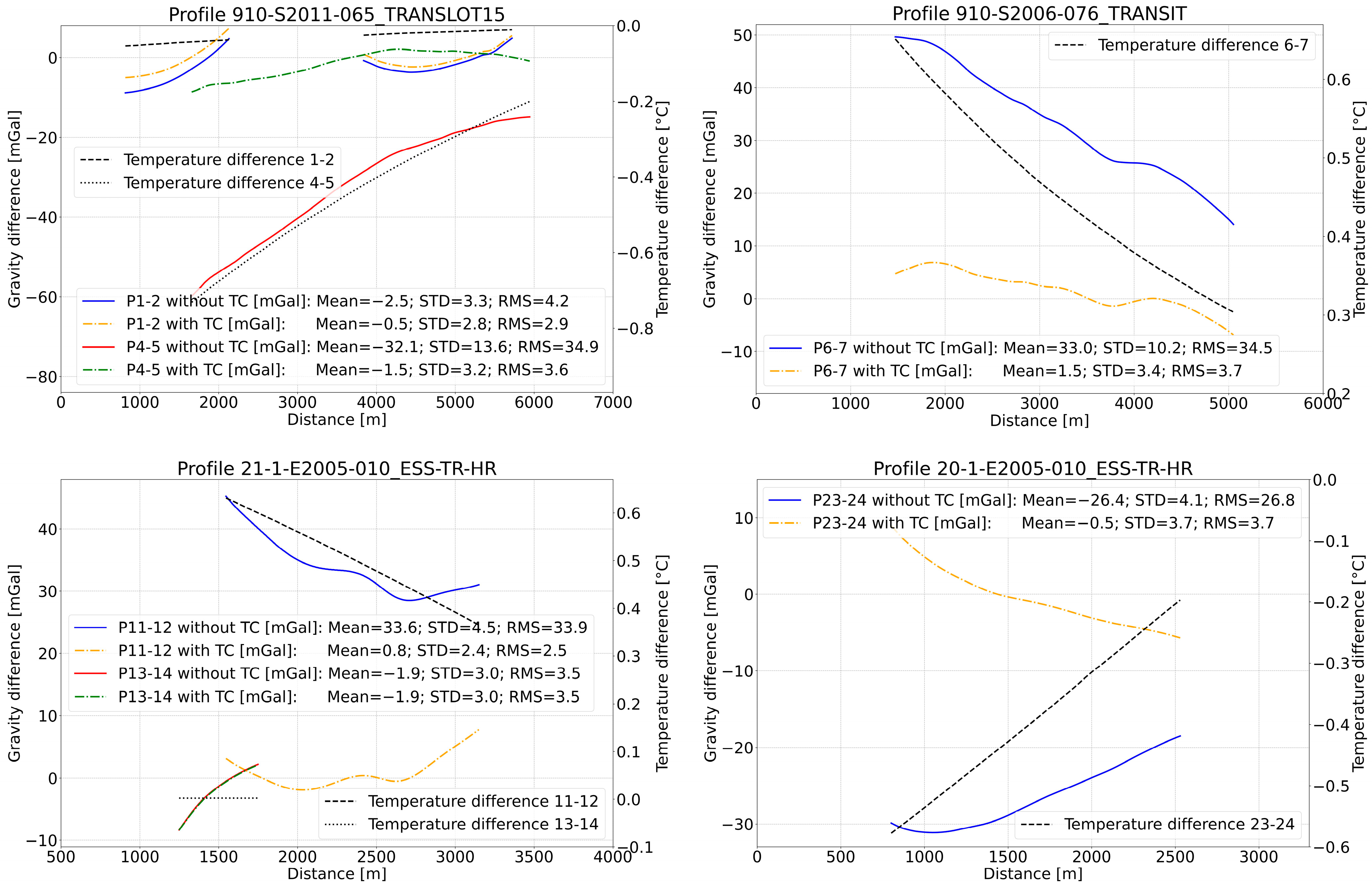
• Utilizing prior knowledge concerning the accelerometer errors, such as those obtained from thermal calibration in the laboratory, to mitigate sensor bias and drift. A simple thermal calibration was carried out, in which the GraviMob gravimeter was subjected to varying temperatures at the gravity point in the GeF laboratory, and the outputs were compared with the available reference gravity value at this point to determine the temperature gradient. This calibrated temperature gradient was used to process data acquired during the GraviMob cruise, but the bias is still significant. This is probably due to the significant difference between the laboratory and actual underwater environments. This calibration method is highly recommended only when used with a climate chamber that subjects the GraviMob system to the actual temperature variations encountered underwater.
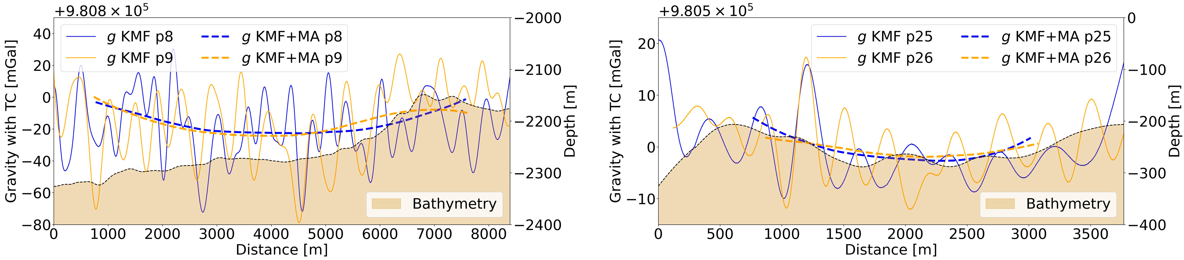
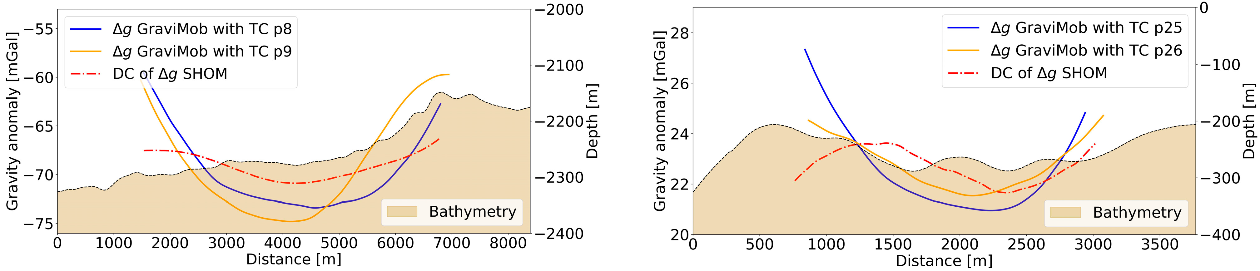
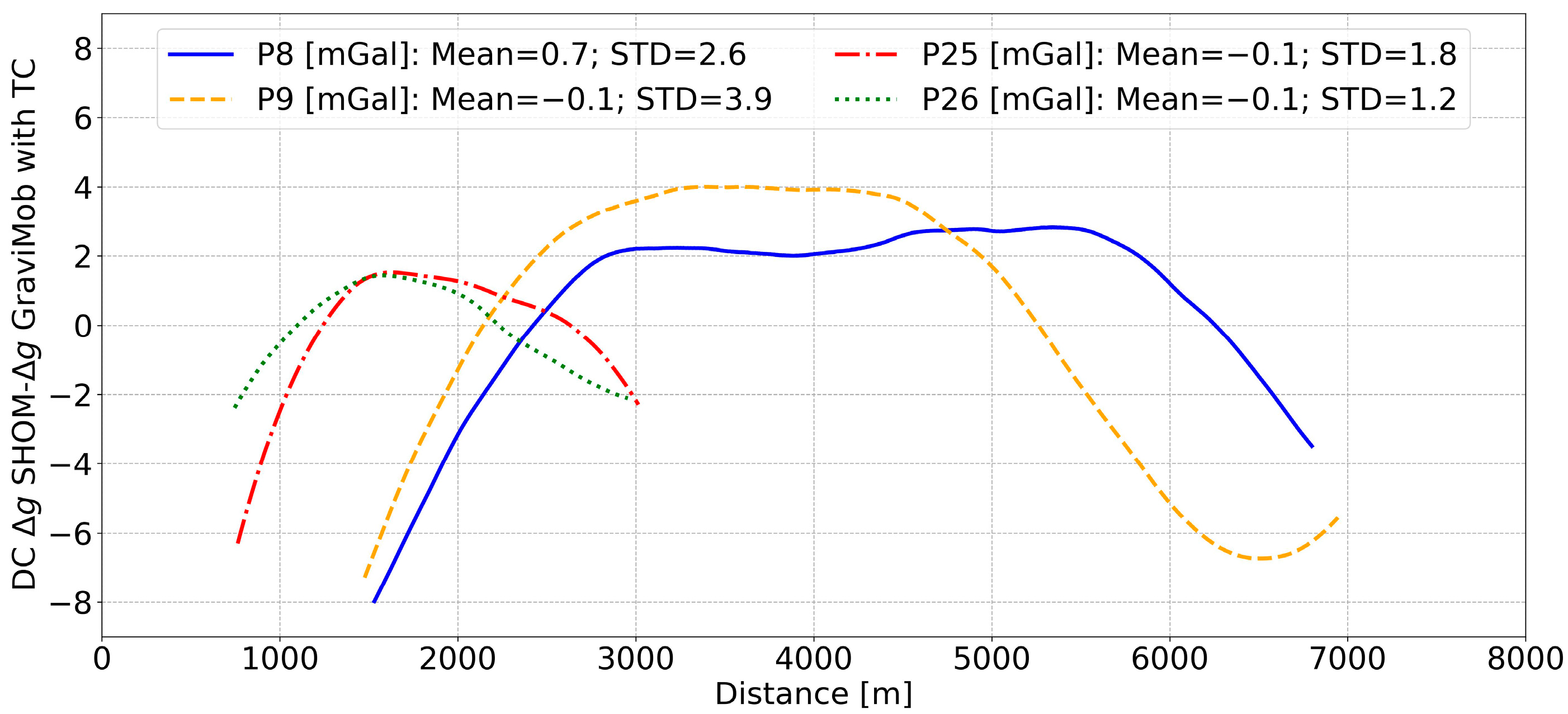
• Employing external reference data, such as those derived from available surface shipborne gravity or from Global Gravity field Models (GGMs), and/or redundant measurements like intersection points or repeated profiles to determine the accelerometer drift and bias present in gravity estimates. This method is often known as the correction technique. However, the availability and spatial resolution of such data are often limited, e.g., the spatial resolution of surface shipborne/GGM-derived gravity is usually lower than that of underwater gravimetry. The terrain effects derived from a high-resolution Digital Bathymetry Model (DBM) can be used to improve the spatial resolution of the surface/GGM-derived gravity data when these data are downward continued (DC) to the measurement depth to be employed as external reference data.

In this study, we focus on the second strategy. To do this, the DC shipborne gravity anomaly is proposed as the external reference data at the measurement depth. Therefore, the downward continuation method, applied through the water layer, will be analysed in detail. Fortunately, the shipborne gravity data have relatively good spatial coverage in the study region. The comparison results between DC shipborne and GraviMob gravity data are used to detect and correct absolute biases as well as drifts. As a result, the temperature correction parameter is determined from these comparison results. To avoid an overcorrection, the corrected sensor bias is considered to be linear over time, while any nonlinear sensor drifts, if present, remain in the GraviMob gravity data. In addition, the internal validation of repeated profiles is also used to estimate the stability of the GraviMob measurements. Here, we report the data processing, temperature correction and validation results of this innovative mobile underwater gravimetry system. In the first part, the data processing procedures to estimate the gravity anomaly at the measurement depth as well as the downward continuation method will be explained. In the second part, the results of the GraviMob cruise will be shown. In the third part, the shipborne gravity data will be downward continued to the measurement depth for comparison with the GraviMob gravity anomaly. Finally, in the last part, the temperature correction results will be validated and discussed.

2. Methods

2.1. GraviMob-Measured Data Processing

The GraviMob system comprises two triads, each with an orthogonal axes in a two-by-two configuration. Each of these triads is equipped with three QFLEX-QA 3000 electrostatic accelerometers, which are produced by the American company Honeywell (Charlotte, NC, USA). This configuration enables the measurement of the three components of the specific force vector [14]. This specific force ($a$) comprises both the gravitational attraction ($g$) and acceleration resulting from the movement of the carrying vehicle ($\ddot{X}$):

$$a=\ddot{X}-g$$

(1)

where the navigation system provides the position and rotation angles of the AUV-transported GraviMob to estimate the acceleration $\ddot{X}$, and thus we can separate this acceleration from the specific force to calculate the gravitational attraction. This navigation system includes: (1) An Inertial Navigation System (INS) provided by iXBlue company; (2) an ultrasonic Doppler velocimeter and an Ultra-Short BaseLine (USBL) positioning system. The former measures the velocity relative to the seafloor and the latter provides the distance and the direction (bearing) between the transceiver installed on the vessel and the acoustic transponder integrated in the AUV. All measurements are used by the INS to determine the AUV’s position; and (3) Global Navigation Satellite System (GNSS) receivers installed on the vessel to ensure precise position determination.

The data processing from GraviMob acceleration measurements and GNSS data has been thoroughly outlined in [14,17]. In this Section, we will present a brief description of this procedure. An Unscented Kalman Filter (UKF) was employed to filter the three components of the gravimetry vector. This filter method is characterized by an evolution model and an observation model. The primary function of the evolution model is to establish the connection between the parameters at a specific time to those at the preceding time. The parameter’s vector ($X_k$) at time $k{T}_e$, with $T_e$ representing the sampling period, is defined as follows:

$$X_k={\left[P\dot{P}\ddot{P}\theta \dot{\theta }\ddot{\theta }g\dot{g}\ddot{g}\right]}_k^T$$

(2)

where $P$ includes the geodetic latitude ($\phi$), geodetic longitude ($\lambda$) and geometric height ($h$) of the AUV. $\dot{P}$ and $\ddot{P}$ are the first and second derivatives of $P$, respectively. $\theta$, $\dot{\theta }$ and $\ddot{\theta }$ are the rotation angles of the vector, and its first and second derivatives, respectively. $g$, $\dot{g}$ and $\ddot{g}$ are the gravity components vector in the navigation frame (n-frame), and its first and second derivatives, respectively. Therefore, there are a total of 27 different parameters to estimate.

The evolution model at successive times $k$ and $k+1$ may then be expressed mathematically as:

$$X_{k+1}=F{X}_k+\Gamma v_k$$

(3)

where $F$ is the state transition matrix defined as a discrete Wiener stochastic process [18], $\Gamma$ is the noise gain matrix and $v_k$ is the discrete-time process noise assumed to be gaussian white noise.

The covariance prediction equation ($P$) is defined as:

$$P_{k+1}=F{P}_k{F}^T+Q_k$$

(4)

where $Q_k$ is the state noise covariance matrix at the instant $k$.

$$Q_k=\Gamma {\sigma }_v^2{\Gamma }^T$$

(5)

where ${\sigma }_v^2$ is the process noise covariance.

The measurement vector $\left(Z_k\right)$ at time $k$ includes the 9 components determined by

$$Z_k={\left[P^{obs}{\theta }^{obs}{a}^{obs}\right]}_k^T$$

(6)

where $a^{obs}$ is the vector of three specific force components which are the average of the two triads. $P^{obs}$ and ${\theta }^{obs}$ are the observed position and orientation parameters, respectively.

The model of observation is then expressed as follows:

$$Z_k=H_k{X}_k+{\omega }_k$$

(7)

where ${\omega }_k$ is the measurement noise.

Let us consider the function $H_k{X}_k$, defined by

$$H_k{X}_k={\left[P^{est}{\theta }^{est}{g}^{est}\right]}_k^T$$

(8)

where $P^{est}$, ${\theta }^{est}$ and $g^{est}$ are the estimated position, orientation, and gravity component parameters, respectively.

The covariance update equation ($P$) is defined as

$$P_{\left(k+1\right)}^{+}=\left[I-W_{\left(k+1\right)}{H}_{\left(k+1\right)}\right]P_{\left(k+1\right)}$$

(9)

where $W_{k+1}$ is the gain matrix of the Kalman filter and $I$ is the identity matrix.

With the matrices $F$ and $Q$ as well as the function $H_k{X}_k$ related to the evolution model (3) and observation model (7), the implementation of the UKF is feasible once an initial state vector $X_0$ and its corresponding covariance matrix are established.

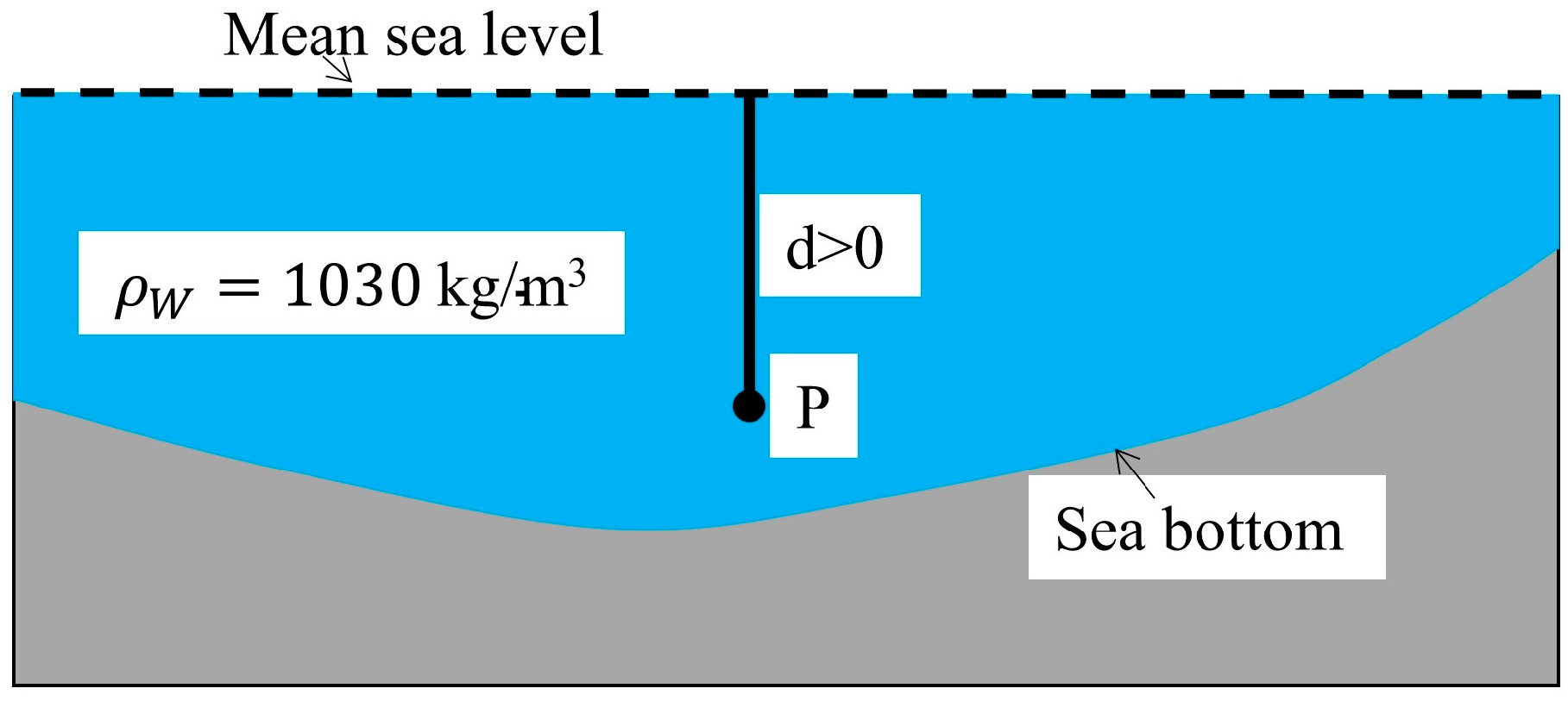
2.2. Free-Air Gravity Anomaly Computation at the Measurement Depth

As mentioned, a true gravity anomaly from the GraviMob measurement system was not determined in [14]. In this Section, we present the formulae for calculating gravity anomalies. Free-air gravity anomalies (${∆g}_{FA}$) are determined by the discrepancy between the observed gravity value ($g$) and normal gravity value at the measured depth $d$ (${\gamma }^d$):

$${∆g}_{FA}=g-{\gamma }^d$$

(10)

where ${\gamma }^d$ was calculated as

$${\gamma }^d=\gamma -4\pi G{\rho }_{W}d-\left(\frac{\partial \gamma }{\partial h}\right)d+\left(\frac{1}{2}\right)\left(\frac{{\partial }^2\gamma }{{\partial h}^2}\right)d^2$$

(11)

where $4\pi G{\rho }_W$ is the water column correction [19], which is used to remove the masses below the geoid (mean sea level) down to the measuring point; $G$ denotes the gravitational constant value; and ${\rho }_W$ is the water density. In this case, a seawater density of 1030 kg/m³ is used. $h$ denotes the ellipsoidal height. $d$ denotes the depth ($d=\left|H^{*}\right|$, with $H^{*}$ as the normal height) (Figure 1).

$\gamma$ denotes the normal gravity at the surface of the reference ellipsoid. This can be calculated by employing Somigliana’s rigorous formula:

$$\gamma =\frac{a{\gamma }_e{cos}^2\phi +b{\gamma }_p{sin}^2\phi }{\sqrt{a^2{cos}^2\phi +b^2{sin}^2\phi }}$$

(12)

$\frac{\partial \gamma }{\partial h}$ is the vertical gradient of normal gravity. It is given by

$$\frac{\partial \gamma }{\partial h}=-2\frac{\gamma }{a}\left(1+f+m-2f\left({sin}^2\phi \right)\right)$$

(13)

$\frac{{\partial }^2\gamma }{{\partial h}^2}$ is the second-order term of the vertical gradient, which can be appreciable at large depths. It is approximated as

$$\frac{{\partial }^2\gamma }{{\partial h}^2}=6\frac{\gamma }{a^2}$$

(14)

where $a$ denotes the semi-major axis of the reference ellipsoid, b denotes the semi-minor axis, ${\gamma }_e$ and ${\gamma }_p$ denote the normal gravity at the equator and at the poles, respectively, $\phi$ denotes the geodetic latitude, $m$ denotes the ratio of centrifugal force to gravity at the equator, and $f$ denotes the geometrical flattening. In this study, all computations were carried out using the parameters of the reference ellipsoid GRS80, which are $a$ = 6,378,137.00 (m), ${\gamma }_e$ = 978,032.67715 (mGal), ${\gamma }_p$ = 983,218.63685 (mGal), $f$ = 1/298.257223563 and $GM$ = 3.986005000109 × 10¹⁴ (m³ s⁻²).

2.3. Downward Continuation Model

As already mentioned in the Introduction, the GraviMob measurements and gravity data gathered on the ship are located at two different altitudes with inhomogeneous spatial resolutions as well as coverage. Therefore, prior to the GraviMob measurement validation using shipborne gravity data, the data need to be DC to the measurement depth at which the GraviMob measurements are taken. The accuracy of GraviMob measurements can be then assessed using the downward continued shipborne data. In this study, the Least-Squares Collocation (LSC) approach [20] adapted to the Remove–Compute–Restore (RCR) method was used as it offers several advantages [21,22,23,24,25]. This method enables interpolation anywhere in the 3D space and input data do not need to be at the same height/depth. A GGM and topographic information from the Residual Terrain Model (RTM) effects were employed to remove/restore low and high frequencies of gravity anomaly before and after DC, respectively. After reduction, we obtain a residual gravity anomaly which has a smaller amplitude and is much smoother than the original gravity anomaly. As a result, using the residual improves our ability to model the Earth’s gravity field due to the smoothing of the field. First, the gravity anomalies derived from EGM2008 up to degree/order (d/o) 2190 [26] were utilized to remove/restore the low frequencies. The terrain effects on the gravity anomaly were determined using Digital Bathymetry Model (DBM) SRTM15arc_plus with a resolution of 15″ [27] to remove/restore the high-frequency parts (i.e., beyond d/o 2190). The residual gravity anomalies were then downward continued to the measurement depth using the LSC method. The downward continuation was carried out according to the diagram in Figure 2, using the GRAFSOFT program [28].

In Figure 2, ${\Delta g}_{FA}^{sur}$ and ${\Delta g}_{res}^{sur}$ are free-air surface shipborne gravity anomalies and their residuals, respectively. ${\Delta g}_{EGM2008}^{sur}$ and ${\Delta g}_{EGM2008}^{depth}$ denote the low frequencies derived from the GGM at the surface of the sea and at the measurement depth, respectively. ${\Delta g}_{RTM}^{sur}$ and ${\Delta g}_{RTM}^{depth}$ denote the topographic effects at the sea surface and at the measurement depth, respectively. Therefore, the low- and high-frequency gravity anomalies from the GGM and from the topographic effects, respectively, are computed at two different depth levels in the remove/restore steps. It should be noted that it is necessary to compute the RTM effects at two different depth levels while not moving the bathymetry surface. ${\Delta g}_{FA}^{DC}$ and ${\Delta g}_{res}^{DC}$ are DC free-air gravity anomalies at the measurement depth and their residual values, respectively.

In the RCR procedure, the RTM effects technique [29] is commonly employed for computing the terrain effects to prevent the high-frequency gravity field noise from topography/bathymetry. Gravity anomalies resulting from the reduction in the RTM effects are generally smoother than those produced by other techniques of terrain reduction [30]. In the process of computing RTM effects, a smooth mean elevation grid is utilized as the reference surface grid for removing topographic masses and filling the deficiencies above and below this smooth reference surface, respectively. A low-pass filter is applied to the detailed topography/bathymetry grid to transform it into a smoother topography/bathymetry grid. The spatial resolution of the refined reference grid should match that of the GGM employed for representing the long wavelengths of the gravity field, i.e., the maximum degree of the GGM employed. Therefore, the advantage of the RTM technique lies in the fact that it only considers the topographic effect that has not been incorporated into the GGM-derived gravity data. As stated by [31], the resolution of the GGMs is connected to their maximum degree $\left(n_{max}\right)$, and can be computed using the following formula:

$${resolution}_{GGM}=\frac{{180}^0}{n_{max}}\left(degree\right)or{resolution}_{GGM}=\frac{20.000\mathrm{km}}{n_{max}}\left(\mathrm{k}\mathrm{m}\right)$$

(15)

The corresponding RTM effect is given by [29]

$${∆g}_{RTM}=2\pi G\rho \left(H-H_{ref}\right)-TC$$

(16)

where $H_{ref}$ denotes the heights derived from the reference and $H$ denotes the heights obtained from the detailed topography/bathymetry grids, $TC$ denotes the classical terrain correction, $G$ denotes the gravitational constant value and $\rho$ represents the density of the Earth’s crust.

2.4. Least-Squares Collocation Method

The traditional collocation formula is as follows [20]:

$$\widehat{s}=C_{\widehat{s}x}{\left[C_{xx}+D\right]}^{-1}x$$

(17)

where $\widehat{s}$ denotes the signal to be determined and $x$ denotes the observation vector. $C_{\widehat{s}x}$ and $C_{xx}$ are the cross- and auto-covariances, respectively. The matrix $D$ expresses the error covariances. This matrix can be determined by employing the available prior noise information. In the context of downward continuation, the signal to be determined is the gravity anomalies at the measurement depth (${∆g}^{bottom}$), and the observations are the shipborne anomalies at the sea surface (${∆g}^{sur}$). Therefore, Equation (17) becomes

$${∆g}^{bottom}=C_{{∆g}^{bottom}{∆g}^{sur}}{\left[C_{{∆g}^{sur}{∆g}^{sur}}+D\right]}^{-1}{∆g}^{sur}$$

(18)

In this method, it is crucial to employ an optimal covariance model that is in reasonable accordance with the spectral properties of the actual gravity field. As we know that the gravity field of Earth follows Kaula’s rule, the covariance model must follow this rule. In the present study, the covariance model developed by R. Forsberg [20], called the attenuated planar logarithmic model, was used. This covariance model was designed for the downward or upward continuation of gravity anomalies. The theoretical covariance for free-air anomalies at two points $P$ and $Q$ at different altitudes is determined by employing function as follows:

$$C\left({∆g}^{H_i},{∆g}^{H_j}\right)=-f{\sum }_{k=0}^3{\alpha }_{k}log\left(D_k+\sqrt{s^2+\left(D_k+H_i+H_j\right)}\right)$$

(19)

where ${∆g}^{H_i}$ and ${∆g}^{H_j}$ denote pairs of gravity points; $H_i$ and $H_j$ are the heights of the pairs of gravity points; ${\alpha }_k$ represents the weight factors (with ${\alpha }_0=1$, ${\alpha }_1=-3$, ${\alpha }_2=3$ and ${\alpha }_3=-1$); and $s$ represents the planar distance between points $i$ and $j$. $D_k$ is the depth value, defined as follows:

$$D_k=D+kT$$

(20)

The scale factor $f$ is defined as

$$f=C_{0}log\frac{{\left(D+T\right)}^3\left(D+3T\right)}{D{\left(D+2T\right)}^3}$$

(21)

$C_0$ denotes the variance of free-air gravity anomalies, e.g., at the sea surface, in this study. $D$ and $T$ are the high- and low-frequency attenuation depth parameters, respectively, $D$ serves as the Bjerhammar sphere depth in the context of spherical collocation. These three parameters are obtained by fitting the empirical covariance to the covariance model. Here, we downward continue the residual gravity anomaly instead of the gravity anomaly. The empirical covariance is computed, employing the residual of the gravity anomalies as follows:

$${cov}_{{∆g}_{res}}\left({\psi }_i\right)=\frac{1}{N_i}{\sum }_{n=1}^{N_i}{\left[{∆g}_{res}\left(P\right){∆g}_{res}\left(P^{\prime }\right)\right]}_n$$

(22)

where ${∆g}_{res}\left(P\right)$ and ${∆g}_{res}\left(P^{\prime }\right)$ are the residual gravity anomalies, ${\psi }_i$ denotes the distance, and their products are computed for all pairs of gravity points ($N_i$) within the specified distance interval as follows:

$${\psi }_i-\frac{∆\psi }{2}\le \psi \le {\psi }_i+\frac{∆\psi }{2}$$

(23)

where $∆\psi$ represents the selected sampling interval distance, which is determined based on the density and the quality of the gravity field data utilized.

3. GraviMob Cruise and Data Processing

3.1. GraviMob Cruise

The GraviMob system was first tested in an underwater gravity survey that took place in March 2016, during the GraviMob-1 cruise, conducted near the southern coast of France in the Mediterranean Sea [32]. The AUV Aster^x was employed as the platform to transport the GraviMob system during this survey. The operation was conducted aboard the vessel Europe of the French Oceanographic Fleet. The main objective was to assess the accuracy of the GraviMob system through (1) self-validation using repeated measuring lines and (2) external validation using the available surface shipborne data. During this cruise, the AUV ran five profiles: two crossover profiles in the eastern zone and three profiles in the western zone (Figure 3). These profiles were measured at different depths with two measuring modes: constant depth and terrain follow-up survey. At each depth, as well as survey mode, the measurement profiles were repeated for internal validation, except for profiles 3 and 10. These measured lines were repeated by lines 1 and 2, and lines 8 and 9, respectively, but at different depths, so these two profiles have no internal validation. Consequently, a total of 26 measuring profiles were obtained in six days. Furthermore, these profiles were all located along surface gravity profiles previously carried out by various ships and cruises. The surface gravity data were provided by SHOM (the French Marine Hydrographic and Oceanographic Service). These were provided to facilitate the external validation of GraviMob data using shipborne gravity, since seafloor gravity data were not previously available in this study region. From now on, the name of the AUV measuring profiles will be designated according to their sequence number in the cruise. The measuring profiles from the GraviMob-1 cruise are given in

Table 1. Statistics of the GraviMob measurement profiles gathered in the Mediterranean Sea in March 2016 and their characteristics.

N°	Date	Shipborne Profile Name	Navigation Mode	Depth or Distance to the Seafloor (m)	Distance (km)
1	18 March 2016	Profile 910-S2011-065_TRANSLOT15	Constant depth	1900	7
2			Constant depth	1900	8
3			Constant depth	1850	8
4	19 March 2016		Terrain follow-up	100	7.5
5			Terrain follow-up	100	7.5
6		Profile 910-S2006-076_TRANSIT	Terrain follow-up	100	8
7	20 March 2016		Terrain follow-up	100	8.5
8			Constant depth	1900	9
9			Constant depth	1900	9
10			Constant depth	1850	3
11	22 March 2016	Profile 21-1-E2005-010_ESS-TR-HR	Terrain follow-up	100	7
12			Terrain follow-up	100	7
13			Constant depth	600	3
14			Constant depth	600	3
15	23 March 2016	Profile 20-2-E2005-010_ESS-TR-HR	Terrain follow-up	85	7
16			Terrain follow-up	85	7.5
17			Constant depth	100	8
18			Constant depth	100	8.5
19			Constant depth	80	7.5
20			Constant depth	80	8
21	24 March 2016	Profile 20-1-E2005-010_ESS-TR-HR	Terrain follow-up	100	4
22			Terrain follow-up	100	4
23			Constant depth	100	4
24			Constant depth	100	4
25			Constant depth	80	4
26			Constant depth	80	4

. The AUV’s velocity was approximatively $v=1.5\mathrm{m}/\mathrm{s}$.

3.2. Data Processing

In this section, we present the procedure to estimate the free-air gravity anomaly at the measurement depth of the GraviMob measurements. As already mentioned, temperature variations caused biases and drifts in the GraviMob measurements, which is why we first use 4 out of 26 profiles to calculate the temperature correction parameter. This parameter is then used to correct the remaining measurement profiles. Profiles 8, 9, 25 and 26, where profiles 8 and 25 are repeated by profiles 9 and 26, respectively, have been selected. All the data were processed to estimate the gravity value. Detailed information about the data processing method employed to estimate the gravity value from GraviMob acceleration measurements and GNSS data can be found in [14]. Finally, the raw gravity for four profiles is given in Figure 4.

In the raw gravity data graphs, we can see that gravity variations can reach 50,000 mGal. In order to reduce this noise, a Kalman filter (KMF) is used to filter the raw gravity measurements. Figure 5 shows the KMF gravity of four profiles (solid lines). A good agreement is visible in the repeated profiles. However, we can also see that after applying the KMF method, non-gravitational components remain. Therefore, a simple moving average (MA) filtering is employed to smooth out the remaining high frequencies. The dashed lines in Figure 5 show the gravity signal after applying the MA filter. The gravity results acquired along the profiles are subsequently analysed to assess the measurement errors and the stability.

To assess the repeatability of the measurements, we compare the gravity signals measured along the round-trip profiles. The discrepancies in gravity between the repeated profiles yield a mean bias value of −4.8 and −7.0 mGal, a standard deviation (STD) of 3.1 and 1.3 mGal and a root mean square (RMS) of 5.7 and 7.1 mGal for profiles 8–9 and 25–26, respectively. These mean values are clearly quite large. We suspect that these biases could be due to temperature variations. This hypothesis is discussed in Section 5.

Using the filtered gravity measured by the GraviMob, Equations (10) and (11) are used to calculate the free-air gravity anomaly at the measurement depth. The final gravity anomalies estimated from the measurements along four profiles are given in Figure 6. The gravity anomalies are around—685 and—545 mGal for profiles 8–9 and 25–26, respectively. At first sight, it seems that these free-air gravity anomalies present a very large bias. Thus, to validate these results, we used downward continued shipborne free-air anomalies. This issue is discussed in the next section.

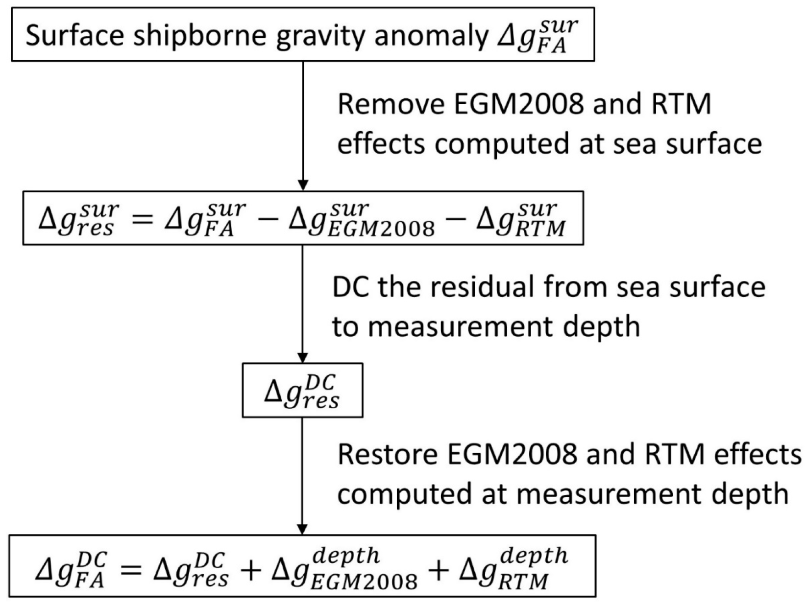
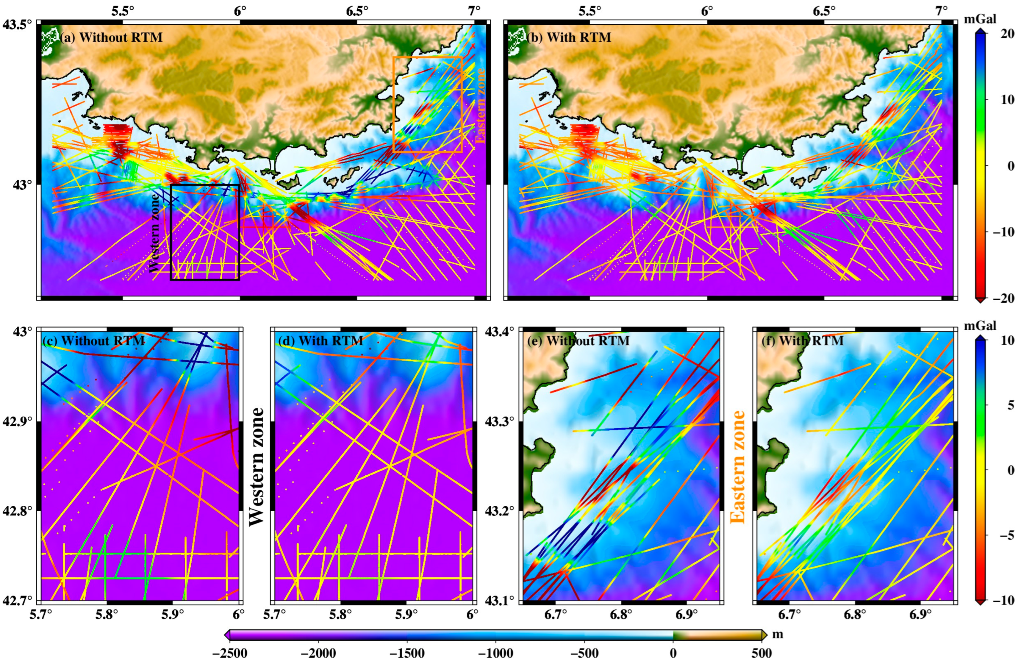
4. Downward Continuation of Shipborne Gravity Data

A set of 167,143 shipborne gravity points was supplied by SHOM. The spatial distribution of the shipborne gravity data is shown in Figure 3 and the related statistics are listed in

Table 2. Statistics of the shipborne gravity anomalies provided by SHOM and their residuals (unit: mGal).

Data	Min	Max	Mean	STD	Zone
${∆g}_{SHOM}^{sur}$	−80.4	63.5	−4.7	36.9	All
${∆g}_{SHOM}^{sur}-{∆g}_{EGM2008}^{sur}$	−38.5	34.4	−3.4	9.5
${∆g}_{RTM}^{sur}$	−13.1	19.2	0.3	4.1
${∆g}_{SHOM}^{sur}-{∆g}_{EGM2008}^{sur}-{∆g}_{RTM}^{sur}$	−28.9	21.2	−3.6	6.8
${∆g}_{SHOM}^{sur}$	−67.7	44.5	−29.3	22.7	Western (black rectangle)
${∆g}_{SHOM}^{sur}-{∆g}_{EGM2008}^{sur}$	−25.9	34.4	−1.7	8.4
${∆g}_{RTM}^{sur}$	−10.9	19.2	−0.3	4.0
${∆g}_{SHOM}^{sur}-{∆g}_{EGM2008}^{sur}-{∆g}_{RTM}^{sur}$	−25.6	18.0	−1.3	5.1
${∆g}_{SHOM}^{sur}$	−51.8	33.8	−12.7	22.0	Eastern (orange rectangle)
${∆g}_{SHOM}^{sur}-{∆g}_{EGM2008}^{sur}$	−33.9	22.3	−1.4	10.0
${∆g}_{RTM}^{sur}$	−13.1	11.1	−0.2	5.0
${∆g}_{SHOM}^{sur}-{∆g}_{EGM2008}^{sur}-{∆g}_{RTM}^{sur}$	−22.2	15.7	−1.1	6.7

. The main problem with on-board gravity measurements is that they are subject to bias due to relative gravimeter drift and incorrect positioning, particularly in older on-board gravity datasets [33]. Therefore, crossover analysis between ship tracks and/or comparison with a satellite altimetry-derived gravity field model have been applied to reduce this drift. On the other hand, gravity data measured at the seafloor are not available in the study region. Thus, the shipborne data are the most satisfactory independent gravity data that we can use to evaluate the GraviMob measurements in this region. As previously mentioned, the GraviMob measurements and surface shipborne gravity data are located at two different altitudes. The shipborne gravity data are therefore downward continued to the measurement depth. Among gravity data processing techniques, DC is considered one of the most unstable procedures [24]. Therefore, to improve the accuracy of the procedure we used the RCR technique, i.e., instead of the gravity anomalies, the residual shipborne gravity anomalies were used.

Until now, a GGM, e.g., EGM2008, has been unable to accurately represent the high-frequency parts of a gravity field, especially in rugged terrain. The reason for this is the omission error of GGMs. According to [34], the omission errors in EGM2008, even at its maximum degree (2190), may reach levels of roughly 10 cm or more in terms of height anomalies in mountainous regions. Therefore, terrain effects were used to complement EGM2008 in the calculation of the gravimetric geoid/quasi-geoid [35], and the geopotential value for the establishment of a modern local [36,37] or international [38] height reference system. The RTM effects also play an important role in the upward/downward continuation procedure used to validate airborne gravity data (see [23,39,40]). These studies indicated that the incorporation of the RTM effects substantially improved the accuracy of the DC airborne gravity anomalies, especially in mountainous areas. Zhao et al. (2018) [23] reported that about ¾ of DC errors are due to the quality of RTM effects. On the other hand, we can hardly see significant improvements when using RTM effects in the relatively flat coastal zones [41]. Wu et al. (2019) [42] stated that the effects of the land’s topography (using SRTM3arc [43]) on the high-frequency gravity field modelled by RTM were found to be more significant than those of the DBM, which was derived using SRTM30arc_plus [44]. This is not surprising, because land topography is much better resolved via the SRTM3arc model than the seafloor topography derived from the DBM. In [45], RTM effects were not used in the RCR procedure to calculate a geoid model for the Mediterranean sea because they make residual gravities slightly larger. Moreover, RTM effects were tested over two coastal zones in [46]. To the north of the island of Sicily, the application of RTM effects partly enhances the residual signal. On the contrary, the residual field is further reduced when removing the RTM effect contributions, on the island of Sulawesi in Indonesia. Obviously, the effectiveness of the RTM effects in the sea domain may differ from one region to another, depending on the spatial resolution and quality of the bathymetry models. Therefore, the RTM effect contributions were investigated in our study region.

To compute the RTM effects, a coarse DBM grid was used for the outer zone instead of a detailed DBM grid to reduce the computing time. In this study, the GRAVSOFT TC program was used to compute the RTM effects, employing a radius of 20 km for the detailed DBM grid and 200 km for the coarse DBM grid. Consequently, coarse and smooth reference DBM grids were generated from the detailed grid in the following manner:

-

We employed a simple averaging to compute the coarse DBM grid (1′ × 1′ grid in the present study) from the detailed DBM grid (SRTM15arc_plus with the resolution of 15″).

-

A moving-average window was then employed to low-pass filter the coarse DBM grid (1′ × 1′) to the required resolution of the reference DBM grid; the required resolution is 9 km (equivalent to the spherical harmonic d/o 2190 of the EGM2008 employed) in the remove–restore procedure for DC shipborne gravity data in this study.

Figure 7 shows the key role of RTM effects in the RCR procedure. It illustrates the comparison of residual gravity anomalies with and without RTM effects in our study region. The differences of ${∆g}_{SHOM}^{sur}-{∆g}_{EGM2008}^{sur}$ in Figure 7a show residual gravity anomalies, with amplitudes reaching 35 mGal and wavelengths primarily in the range of 10–15 km. Note that 20 km is equivalent to the minimum wavelengths that can be resolved by EGM2008 (with a resolution of 5′). Figure 7a shows numerous peak structures corresponding to the bathymetry in the background, especially in the profiles near the coast, where bathymetry is relatively rough. Figure 7b shows the discrepancies between shipborne gravity anomalies and the EGM2008 enhanced by the RTM effects-derived gravity anomalies. Comparison with Figure 7a demonstrates a significant improvement when RTM effects are used to reduce the omission errors in EGM2008. The RTM effects in gravity anomalies reduce nearly all peak structures with amplitudes ranging from 25 to 35 mGal to levels of 15–25 mGal or lower. However, some structures are still visible in Figure 7b. This may be due to several reasons, e.g., shipborne gravity errors, EGM2008 commission errors or RTM gravity anomaly errors, but in our opinion, it is mainly due to the quality of the used DBM and the density assumed in the calculation of the RTM effects. In this study, a seawater density of 1030 kg/m³ was used.

The descriptive statistics of the ${∆g}_{SHOM}^{sur}-{∆g}_{EGM2008}^{sur}$ and ${∆g}_{SHOM}^{sur}-{∆g}_{EGM2008}^{sur}-{∆g}_{RTM}^{sur}$ in Table 2 indicate a reduction in the STD of these differences from 9.5 to 6.8 mGal. This corresponds to an improvement rate of 28.4%. Upon the application of both reductions from EGM2008 and RTM effects, the residual gravity anomaly signal becomes significantly smoother, with reduced amplitudes. The initial absolute range (maximum–minimum value) of 145 mGal is reduced to 75 and 50 mGal when only EGM2008 and EGM2008 enhanced with RTM effects are used, respectively. This illustrates that enhancing EGM2008 with RTM effects provides considerably more accurate gravity anomalies compared to EGM2008 alone in this region.

To better see the improvement when using the RTM effects in the RCR procedure, we show the results of our two experimental measurement zones. Figure 7d,f show that most of the peak structure was removed when RTM effects were used. The peak structures are clearly visible in the eastern zone in Figure 7e (using EGM2008 alone) where the DBM is rougher. The STDs decrease from 8.4 and 10.0 to 5.1 and 6.7 mGal for the western and eastern zones, respectively. These equate to an improvement rate of 37.5 and 33.0% for the western and eastern zones, respectively. It is worth noting that the reduced gravity anomalies have small mean values (about 1 mGal) in these two zones.

These results suggest that EGM2008 (from degree 2 to 2190) combined with RTM effects (from degree 2191 to 43,200, equivalent to the 15″ resolution of SRTM15arc_plus) should be used for the RCR technique in the DC shipborne gravity procedure.

The residual gravity anomalies were DC from the sea surface to the locations of existing GraviMob measurements using the LSC method. The DC shipborne gravity anomalies were then obtained through the restoration of EGM2008 and the RTM effects calculated at the specific depth levels where the GraviMob observations were carried out. The DC shipborne gravity anomalies are shown in Figure 6 (red dash–dot lines). We can see in Figure 6 that the gravity anomaly trends revealed by GraviMob closely align with the expected trends obtained from the DC shipborne gravity data. However, a very large bias is also visible. The discrepancies between the DC shipborne and GraviMob gravity anomalies are shown in Figure 8 and listed in

Table 3. Statistics of temperature differences between the sensor temperature and T₀ = 23.8 °C, the temperature at which the internal calibration parameters of the GraviMob system were determined, and gravity anomaly differences between DC shipborne (SHOM) and GraviMob data without temperature correction, for four profiles.

	Profile 8	Profile 9	Profile 25	Profile 26
Mean value of gravity anomaly differences between DC shipborne (SHOM) and GraviMob (mGal) measurements [1]	623.8	618.5	573.3	566.2
Mean value of differences between sensor temperature and T0 (°C) [2]	9.312	9.243	8.566	8.463
[1]/[2] (mGal/°C)	66.989	66.916	66.927	66.903
Mean value of [1]/[2] (mGal/°C)	66.934

Note: T₀ is the temperature at which the internal calibration parameters of the GraviMob system were determined.

. These differences have a large mean bias of 623.8, 618.5, 573.3 and 566.2 mGal for profiles 8, 9, 25 and 26, respectively. They are even much larger than the bias found in [14] (210 mGal). Furthermore, these mean bias values differ significantly, especially when comparing the profiles of two different days (about 50 mGal, 620 vs. 570 mGal for March 20 and 24, respectively). This will be addressed in the next section.

5. Temperature Correction: Results and Discussion

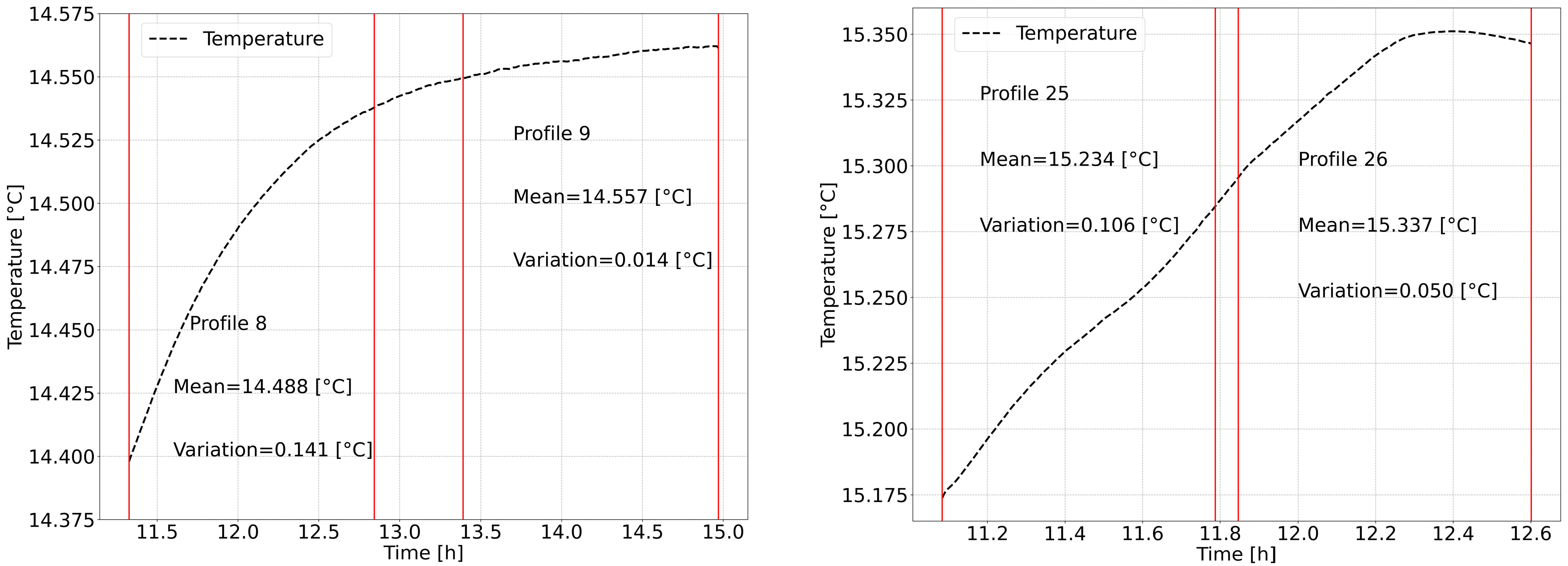
5.1. Temperature Correction Parameter Determination

The GraviMob system is equipped with six temperature sensors to determine the actual temperature inside the system. The temperature for four profiles, averaged over the six sensors, is shown in Figure 9. The internal GraviMob temperature increases gradually over time, although the ambient temperature at the sea bottom is relatively stable. This occurs because of the heat produced by the internal electronic components. The temperature is more stable during the last measurement profiles of the day, i.e., profiles 9 and 26. The largest temperature variation, 0.141 °C, was seen in profile 8. The difference in average temperature between the two days is significant, about 0.8 °C, from 14.5 °C on 20 March to 15.3 °C on 24 March. This difference in temperature explains the large difference in mean bias values between the DC shipborne and GraviMob gravity anomalies for the four profiles on two different days (about 50 mGal, see Figure 8). It should be noted that this actual temperature significantly differs from the temperature at which the internal calibration parameters were determined in the GeF laboratory, T₀ = 23.8 °C [17]. These differences are listed in Table 3.

The gravity and temperature differences between repeated profiles are shown in Figure 10. As already discussed in Section 3.2, there is a large mean bias for gravity differences in the repeated profiles. Furthermore, except for the end of profiles 8–9 (around the location, at a distance of 6 km, where the DBM changes, see Figure 5), a good linear correlation between the gravity (blue solid lines) and temperature differences (black dashed lines) can be seen in Figure 10. The change in DBM could be the cause of the gravity signal change in profile 9 from the location at a distance of 6 km (see Figure 5). This non-temperature-affected component explains the nonlinearity between the gravity and temperature differences at the end of the repeated profiles 8–9. The good correlation reveals that the mean bias of the gravity differences might be due to temperature change. We will therefore address the problem of resolving the influence of temperature changes on GraviMob measurements.

First, a temperature-related gradient for the GraviMob system can be determined for each profile as

$$Gradient=\frac{MeangravityanomalydifferencesbetweenDWCshipborneandGraviMob}{Meantemperaturedifferencesbetweensensortemperatureand{T}_0}$$

(24)

The gradients of the four profiles are listed in Table 3. Good agreement is obtained for the gradients of the four profiles. Therefore, a simple average is then used to determine the ${Gradient}_{average}$ for correcting temperature variation. A gradient of 66.934 mGal/°C is found. This gradient is larger than that determined in the thermal laboratory calibration procedure on the gravity point at the GeF laboratory (62.84 mGal/°C, see [17]). Obviously, with such a large gradient, to achieve an accuracy of less than 1 mGal it is necessary to maintain the temperature stability to within 0.01 °C. Otherwise, temperature correction is required. The temperature change is relatively linear (see Figure 10), so to avoid over-correction we proceed to correct the temperature as

$$g_{GraviMob}^{cor}=g_{GraviMob}+\left(T_0-T\right)\times {Gradient}_{average}$$

(25)

where $T$ is the sensor temperature measured by the GraviMob system. $g_{GraviMob}$ and $g_{GraviMob}^{cor}$ are gravity measurements and the gravity-corrected temperature.

The GraviMob gravity values after applying temperature corrections are shown in Figure 11. In comparison with Figure 5, the use of temperature corrections gives a much better agreement between the repeated profiles. Gravity differences after applying temperature corrections between the repeated profiles are shown in Figure 10 (orange dash–dot lines). After applying temperature corrections, there is no mean bias remaining in the repeated profiles (−0.3 and 0.2 mGal vs. −4.8 and −7.0 mGal when no temperature correction is applied for the repeated profiles 8–9 and 25–26, respectively). This leads to a significant reduction in RMS (from 5.7 to 2.9 mGal and from 7.1 to 1.1 mGal for the repeated profiles 8–9 and 25–26, respectively). Temperature-affected drifts are also slightly reduced (reduction of 0.2 mGal in STD for each repeated profile). These are profiles with relatively stable temperatures, so the drift is not strong. For profiles where the temperature changes significantly, this effect will be more obvious. The non-temperature-affected component explains the large difference that remains at the end of profiles 8–9.

The free-air gravity anomaly is then calculated via the subtraction of the normal gravity from the filtered gravity data after applying the temperature correction (using Equations (10) and (11)). The GraviMob gravity anomaly is indicated in Figure 12 (solid lines). It is evident that the GraviMob gravity anomaly is now much closer to the DC shipborne gravity anomaly (both in trend and magnitude).

Figure 13 shows the discrepancies between the DC shipborne and the GraviMob gravity anomalies after applying temperature correction to the four profiles. These differences have a mean value varying from −0.1 to 0.7 mGal and a STD varying from 1.2 to 3.9 mGal. Large differences appear at the beginning and end of each profile. This is due to the edge effect of the filter. Clearly, we need to take this into account for future cruises, i.e., the profiles need to be longer than the target area. The results demonstrate the effectiveness of the temperature correction method that was applied. In the next section, the remaining profiles will be processed in the same way.

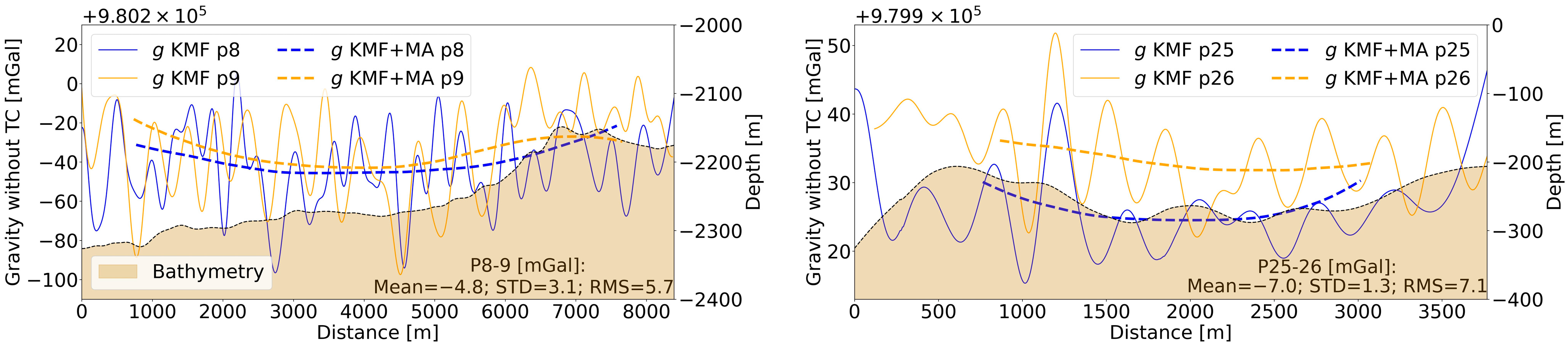
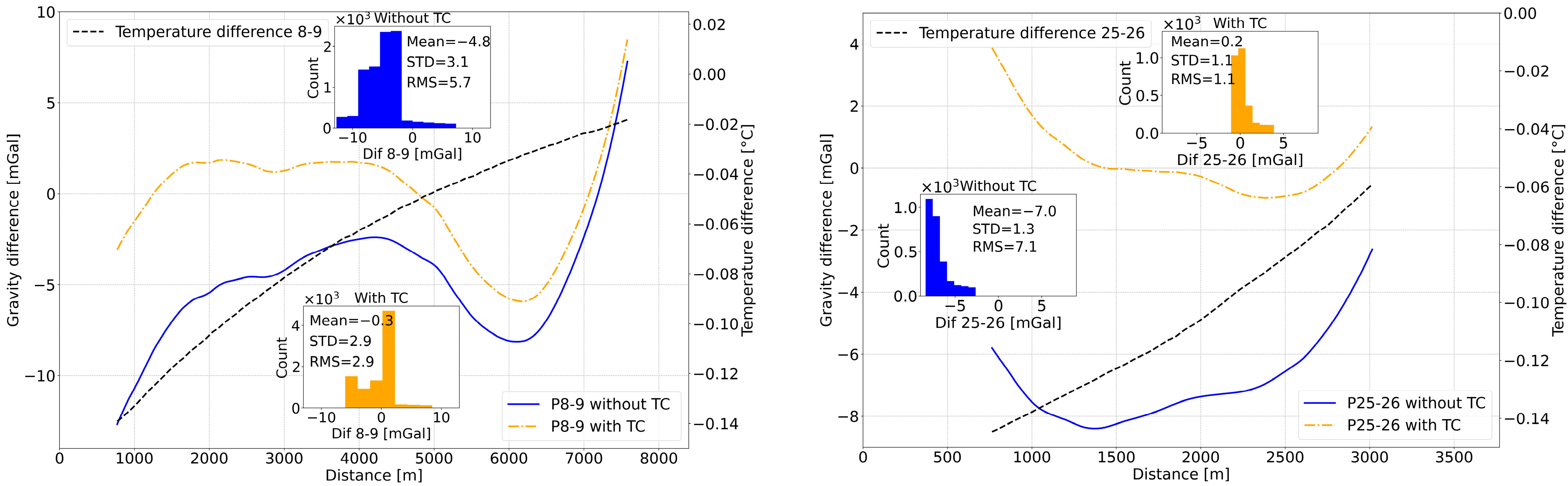
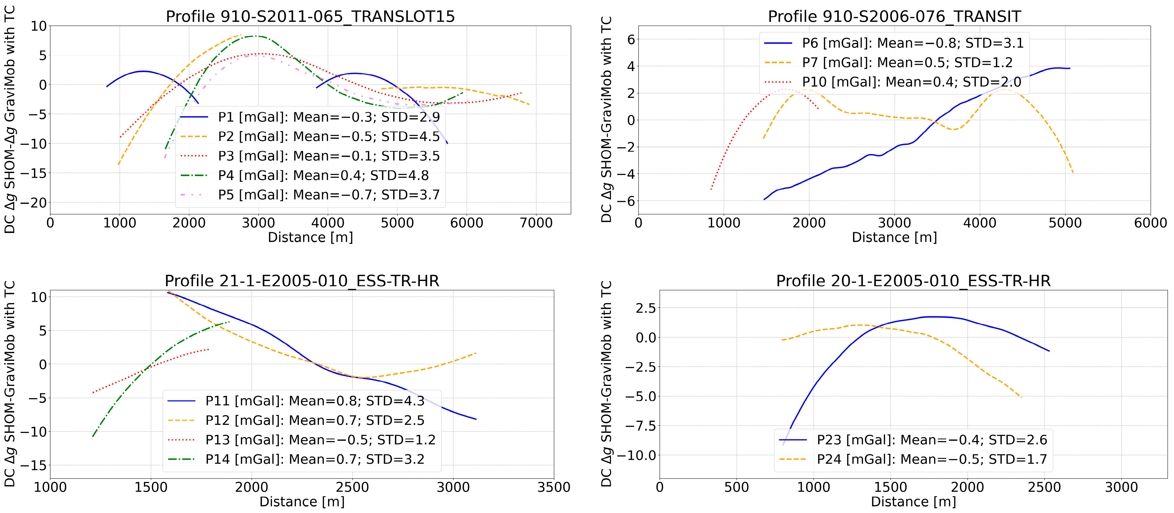
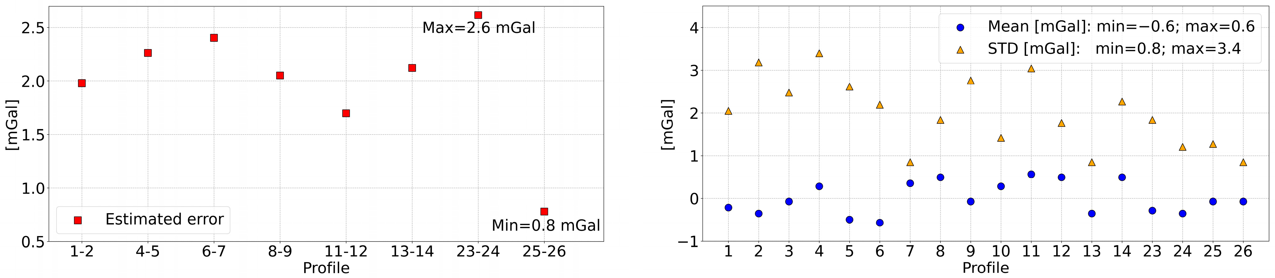
5.2. Validation Results for the Remaining Profiles

We applied the same procedure to the remaining profiles. However, all six profiles from 23 March (profiles 15, 16, 17, 18, 19 and 20) could not be processed due to poor measurement quality (due to accelerometer saturation and/or the interruption of navigation data recording). Similarly, the first two profiles of 24 March (profiles 21 and 22) could not be processed. These two profiles were measured in a terrain follow-up mode and the DBM is relatively rough due to the presence of several deep canyons (see Figure 5 on the left). As a result, only 14 of the remaining profiles were processed, which means that 18 out of 26 were successfully processed (69.2%). This is a good score as the navigation conditions for the AUV in the second part of the cruise (the eastern zone) are particularly difficult due to the rough terrain and to strong currents. Note that during processing for profiles 6, 7, 11 and 12, we had to remove the parts where the DBM is rough (due to the bad quality of the measurements). These are profiles measured using the terrain follow-up mode. One conclusion is that the constant depth survey mode is preferable for the GraviMob system.

The internal validation results are indicated in Figure 14. It should be noted that the same filter parameters were used for each repeated profile. A good correlation between the gravity differences without temperature correction (solid lines) and temperature differences (black lines) is generally visible. As seen before, for the first profiles of each day where the temperature is much less stable, the temperature-affected drifts are significantly reduced due to the temperature correction (dash–dot lines). For example, the STD of repeated profiles 4–5 (profile 4 is the first profile of 19 March, see Table 1) has been reduced from 13.6 to 3.2 mGal, that of the repeated profiles 6–7 (profile 7 is the first profile of 20 March) from 10.2 to 3.4 mGal, and that of the repeated profiles 11–12 (profile 11 is the first profile of 21 March) from 4.5 to 2.4 mGal. The difference after applying the temperature correction across all repeated profiles has a mean bias value varying from −1.9 to 1.5 mGal and a STD varying from 1.1 to 3.7 mGal. Based on the law of error propagation, which assumes the statistical independence of errors, the accuracy of a single observation profile is given by the STD of the differences divided by $\sqrt{2}$. This gives an estimated error ranging from 0.8 to 2.6 mGal for the GraviMob gravity signal. This is a highly satisfactory result. It is noteworthy that the repeated profiles 6–7 were measured on two different days, with profile 6 being the last profile of 19 March and profile 7 being the first profile of 20 March (see Table 1). Figure 14 on the upper left shows that the mean, STD and RMS values for this pair significantly decrease from 33.0, 10.2 and 34.5 mGal to 1.5, 3.4 and 3.7 mGal, respectively, when temperature correction is used. Thus, we can successfully process repeated profiles measured on two different days. This demonstrates the stability of the GraviMob measurements.

To assess the stability of the gravity measurements made during the dives, the mean values of the gravity differences in each repeated profile are compared (see Figure 15). The variation of the mean values (maximum–minimum value), 65.7 mGal, reduces to 3.4 mGal when temperature correction is used. The mean and STD of the mean values decrease from −1.3 to −0.3 mGal and from 22.4 to 1.0 mGal, respectively, when temperature correction is applied. After applying the correction, the STD on the mean values is very small (1.0 mGal), 22 times better than when no temperature correction is applied. These results demonstrate the good stability of the GraviMob system as well as the correctness of the proposed temperature correction method. The results indicated that if a stabilised sensor temperature is unavailable, a temperature correction is necessary to obtain gravity measurements at the mGal level.

The discrepancy between the DC shipborne and the temperature-corrected GraviMob gravity anomalies is shown in Figure 16. This difference has a mean value varying from −0.8 to 0.8 mGal and a STD varying from 1.1 to 4.8 mGal for all repeated profiles. As discussed, large differences also come from the beginning and end of each profile due to filtering limitations. Considering the shipborne gravity data errors plus the errors of the DC procedure, we assume that the error of the DC shipborne data is equivalent to the error of the GraviMob data. Similar to the internal validation, the mean and STD values are given by dividing by $\sqrt{2}$. This thus gives an STD ranging from 0.8 to 3.4 mGal and a mean bias value varying from −0.6 to 0.6 mGal.

6. Conclusions and Perspectives

The underwater gravity measurements carried out during the GraviMob project have been studied, starting from the fundamental processing of the gravity measurements to the final validation of free-air gravity anomalies. A complete software for these processing procedures has been developed. The processing procedure of the GraviMob measurements has yielded several critical findings. First, bias and drift may be compensated for using temperature correction. A strong temperature-related gradient estimated at 69.934 mGal/°C justifies the relevance of the correction. Second, regarding the validation results, the STD of the gravity differences at repeated profiles varies from 1.1 to 3.7 mGal. This implies that the accuracy for the GraviMob underwater gravimetry ranges from 0.8 to 2.6 mGal, based on the law of error propagation. A good stability of the GraviMob measurements was obtained after applying a temperature correction, with the STD on the mean values of the gravity differences at repeated profiles reducing to 1.0 mGal. The DC surface shipborne data can be used to externally validate the GraviMob free-air gravity anomalies. The discrepancies between the DC shipborne and GraviMob gravity anomalies have an STD ranging from 0.8 to 3.4 mGal and a mean bias value varying from −0.6 to 0.6 mGal. A summary of these comparison results is shown in Figure 17. Good agreements have been achieved on repeated lines, and between GraviMob and DC shipborne gravity anomalies. The findings indicated that, if a stabilised sensor temperature is unavailable, a temperature correction is necessary to obtain gravity observations at the mGal level. Last, the terrain follow-up survey mode can only be applied where the DBM is relatively flat. So, the constant depth survey mode is preferable for future cruises.

Better accuracy could be achieved in the future with the GraviMob system. The temperature control could be improved. For example, the wide variations in temperature over the first few profiles of each day indicate that several hours are needed to stabilise the temperature inside the GraviMob system before data are officially recorded, i.e., 1–2 h. However, even following a long warm-up period, temperature variations of the in-diving accelerometer must be taken into account, given that the sphere temperature can change during the dive due to seawater temperature variations. With a required temperature variation less than 0.01 °C, a temperature stabilisation box could be proposed. Research on solutions to improve the accuracy of the AUV navigation and orientation is also required. For the GraviMob-1 cruise, the horizontal and vertical position accuracies achieved are at 1 to 2.5 m and 0.3 m, respectively. In February 2022, Exail carried out a test campaign to check the accuracy of AUV positioning using the Spare-LBL (Long BaseLine acoustic positioning system) solution at a depth of 1000–3000 m. The horizontal accuracy achieved was better than 0.5 m (personal communication). This result is promising for improvement in the accuracy of the GraviMob corrections. On the other hand, there is a need for the improvement of GraviMob data processing. For instance, the utilization of a Gaussian filter could be considered for processing instead of a simple moving average. Selecting an optimal combination between GGM and RTM effects can also improve the accuracy of the DC procedure, thereby improving the accuracy of the external reference data. The crossover points can also be used as control points to adjust the drifts, which should also be noted when planning future test cruises. In conclusion, GraviMob-1 turned out to be a very successful underwater gravimetry cruise, serving as a first step for the preparation of future cruises with the sensor, for instance, in the Atlantic Ocean.

References

1. Sandwell, D.T.; Müller, R.D.; Smith, W.H.F.; Garcia, E.; Francis, R. New global marine gravity model from CryoSat-2 and Jason-1 reveals buried tectonic structure. Science 2014, 346, 65–67. [Google Scholar] [CrossRef] [PubMed]
2. Vu, D.T.; Bonvalot, S.; Bruinsma, S.; Bui, L.K. A local lithospheric structure model for Vietnam derived from a high-resolution gravimetric geoid. Earth Planets Space 2021, 73, 92. [Google Scholar] [CrossRef]
3. Watts, A.B.; Talwani, M. Gravity Anomalies Seaward of Deep-Sea Trenches and their Tectonic Implications. Geophys. J. Int. 1974, 36, 57–90. [Google Scholar] [CrossRef]
4. Hall, S.A.; Casey, J.F.; Elthon, D.L. A possible explanation of gravity anomalies over mid-ocean ridges. J. Geophys. Res. Solid Earth 1986, 91, 3724–3738. [Google Scholar] [CrossRef]
5. Carbone, D.; Zuccarello, L.; Messina, A.; Scollo, S.; Rymer, H. Balancing bulk gas accumulation and gas output before and during lava fountaining episodes at Mt. Etna. Sci. Rep. 2015, 5, 18049. [Google Scholar] [CrossRef] [PubMed]
6. Montagner, J.-P.; Juhel, K.; Barsuglia, M.; Ampuero, J.P.; Chassande-Mottin, E.; Harms, J.; Whiting, B.; Bernard, P.; Clévédé, E.; Lognonné, P. Prompt gravity signal induced by the 2011 Tohoku-Oki earthquake. Nat. Commun. 2016, 7, 13349. [Google Scholar] [CrossRef] [PubMed]
7. Nabighian, M.N.; Ander, M.E.; Grauch, V.J.S.; Hansen, R.O.; LaFehr, T.R.; Li, Y.; Pearson, W.C.; Peirce, J.W.; Phillips, J.D.; Ruder, M.E. Historical development of the gravity method in exploration. Geophysics 2005, 70, 63ND–89ND. [Google Scholar] [CrossRef]
8. Shinohara, M.; Yamada, T.; Ishihara, T.; Araya, A.; Kanazawa, T.; Fujimoto, H.; Uehira, K.; Tsukioka, S.; Omika, S.; Iizasa, K. Development of an underwater gravity measurement system using autonomous underwater vehicle for exploration of seafloor deposits. In Proceedings of the OCEANS 2015, Genova, Italy, 18–21 May 2015; pp. 1–7. [Google Scholar]
9. National Research Council (NRC). Airborne Geophysics and Precise Positioning: Scientific Issues and Future Directions; National Academies Press: Washington, DC, USA, 1995; ISBN 978-0-309-05183-5. [Google Scholar]
10. Sasagawa, G.S.; Crawford, W.; Eiken, O.; Nooner, S.; Stenvold, T.; Zumberge, M.A. A new sea-floor gravimeter. Geophysics 2003, 68, 544–553. [Google Scholar] [CrossRef]
11. Kinsey, J.C.; Tivey, M.A.; Yoerger, D.R. Dynamics and navigation of autonomous underwater vehicles for submarine gravity surveying. Geophysics 2013, 78, G55–G68. [Google Scholar] [CrossRef]
12. Ishihara, T.; Shinohara, M.; Fujimoto, H.; Kanazawa, T.; Araya, A.; Yamada, T.; Iizasa, K.; Tsukioka, S.; Omika, S.; Yoshiume, T.; et al. High-resolution gravity measurement aboard an autonomous underwater vehicle. Geophysics 2018, 83, G119–G135. [Google Scholar] [CrossRef]
13. Zhang, Z.; Li, J.; Zhang, K.; Yu, R. Experimental Study on Underwater Moving Gravity Measurement by Using Strapdown Gravimeter Based on AUV Platform. Mar. Geod. 2021, 44, 108–135. [Google Scholar] [CrossRef]
14. Verdun, J.; Roussel, C.; Cali, J.; Maia, M.; D’Eu, J.-F.; Kharbou, O.; Poitou, C.; Ammann, J.; Durand, F.; Bouhier, M.-É. Development of a Lightweight Inertial Gravimeter for Use on Board an Autonomous Underwater Vehicle: Measurement Principle, System Design and Sea Trial Mission. Remote Sens. 2022, 14, 2513. [Google Scholar] [CrossRef]
15. Jensen, T.E.; Olesen, A.V.; Forsberg, R.; Olsson, P.-A.; Josefsson, Ö. New Results from Strapdown Airborne Gravimetry Using Temperature Stabilisation. Remote Sens. 2019, 11, 2682. [Google Scholar] [CrossRef]
16. Hofmann-Wellenhof, B.; Moritz, H. Physical Geodesy, 2nd ed.; Springer: Berlin/Heidelberg, Germany, 2006; ISBN 978-3-211-33544-4. [Google Scholar]
17. Roussel, C. Expérimentation d’un Gravimètre Mobile Léger et Novateur Pour la Mesure du Champ de Gravité en Fond de Mer. Ph.D. Thesis, Conservatoire National des Arts et Métiers, Paris, France, 2017. [Google Scholar]
18. Bar-Shalom, Y.; Li, X.R.; Kirubarajan, T. Estimation with Applications to Tracking and Navigation, 1st ed.; Wiley-Interscience: New York, NY, USA, 2001; ISBN 978-0-471-41655-5. [Google Scholar]
19. Zumberge, M.A.; Ridgway, J.R.; Hildebrand, J.A. A towed marine gravity meter for near-bottom surveys. Geophysics 1997, 62, 1386–1393. [Google Scholar] [CrossRef]
20. Forsberg, R. A new covariance model for inertial gravimetry and gradiometry. J. Geophys. Res. Solid Earth 1987, 92, 1305–1310. [Google Scholar] [CrossRef]
21. Alberts, B.; Klees, R. A comparison of methods for the inversion of airborne gravity data. J. Geod. 2004, 78, 55–65. [Google Scholar] [CrossRef]
22. Barzaghi, R.; Borghi, A.; Keller, K.; Forsberg, R.; Giori, I.; Loretti, I.; Olesen, A.V.; Stenseng, L. Airborne gravity tests in the Italian area to improve the geoid model of Italy. Geophys. Prospect. 2009, 57, 625–632. [Google Scholar] [CrossRef]
23. Zhao, Q.; Xu, X.; Forsberg, R.; Strykowski, G. Improvement of Downward Continuation Values of Airborne Gravity Data in Taiwan. Remote Sens. 2018, 10, 1951. [Google Scholar] [CrossRef]
24. Varga, M.; Pitoňák, M.; Novák, P.; Bašić, T. Contribution of GRAV-D airborne gravity to improvement of regional gravimetric geoid modelling in Colorado, USA. J. Geod. 2021, 95, 53. [Google Scholar] [CrossRef]
25. Bidel, Y.; Zahzam, N.; Bresson, A.; Blanchard, C.; Bonnin, A.; Bernard, J.; Cadoret, M.; Jensen, T.E.; Forsberg, R.; Salaun, C.; et al. Airborne Absolute Gravimetry With a Quantum Sensor, Comparison With Classical Technologies. J. Geophys. Res. Solid Earth 2023, 128, e2022JB025921. [Google Scholar] [CrossRef]
26. Pavlis, N.K.; Holmes, S.A.; Kenyon, S.C.; Factor, J.K. The development and evaluation of the Earth Gravitational Model 2008 (EGM2008). J. Geophys. Res. Solid Earth 2012, 117, B04406. [Google Scholar] [CrossRef]
27. Tozer, B.; Sandwell, D.T.; Smith, W.H.F.; Olson, C.; Beale, J.R.; Wessel, P. Global Bathymetry and Topography at 15 Arc Sec: SRTM15+. Earth Space Sci. 2019, 6, 1847–1864. [Google Scholar] [CrossRef]
28. Forsberg, R.; Tscherning, C.C. An Overview Manual for the GRAVSOFT Geodetic Gravity Field Modelling Programs; Technical University of Denmark (DTU): Kongens Lyngby, Denmark, 2008; Available online: https://ftp.space.dtu.dk/pub/RF/ (accessed on 21 January 2024).
29. Forsberg, R. A Study of Terrain Reductions, Density Anomalies and Geophysical Inversion Methods in Gravity Field Modelling; Department of Geodetic Science and Surveying, Ohio State University: Columbus, OH, USA, 1984. [Google Scholar]
30. Sansò, F.; Sideris, M.G. (Eds.) Geoid Determination: Theory and Methods; Lecture Notes in Earth System Sciences; Springer: Berlin/Heidelberg, Germany, 2013; ISBN 978-3-540-74699-7. [Google Scholar]
31. Torge, W.; Müller, J. Geodesy; De Gruyter: Berlin, Germany, 2012; ISBN 978-3-11-025000-8. [Google Scholar]
32. Maia, M. GRAVIMOB Cruise, L’Europe R/V. 2016. SEANOE. Available online: https://campagnes.flotteoceanographique.fr/campagnes/16011200/ (accessed on 1 August 2023).
33. Wessel, P.; Watts, A.B. On the accuracy of marine gravity measurements. J. Geophys. Res. Solid Earth 1988, 93, 393–413. [Google Scholar] [CrossRef]
34. Hirt, C.; Featherstone, W.E.; Marti, U. Combining EGM2008 and SRTM/DTM2006.0 residual terrain model data to improve quasigeoid computations in mountainous areas devoid of gravity data. J. Geod. 2010, 84, 557–567. [Google Scholar] [CrossRef]
35. Vu, D.T.; Bruinsma, S.; Bonvalot, S. A high-resolution gravimetric quasigeoid model for Vietnam. Earth Planets Space 2019, 71, 65. [Google Scholar] [CrossRef]
36. Vu, D.T.; Bruinsma, S.; Bonvalot, S.; Bui, L.K.; Balmino, G. Determination of the geopotential value on the permanent GNSS stations in Vietnam based on the Geodetic Boundary Value Problem approach. Geophys. J. Int. 2021, 226, 1206–1219. [Google Scholar] [CrossRef]
37. Vu, D.T.; Bruinsma, S.; Bonvalot, S.; Remy, D.; Vergos, G.S. A Quasigeoid-Derived Transformation Model Accounting for Land Subsidence in the Mekong Delta towards Height System Unification in Vietnam. Remote Sens. 2020, 12, 817. [Google Scholar] [CrossRef]
38. Sánchez, L.; Ågren, J.; Huang, J.; Wang, Y.M.; Mäkinen, J.; Pail, R.; Barzaghi, R.; Vergos, G.S.; Ahlgren, K.; Liu, Q. Strategy for the realisation of the International Height Reference System (IHRS). J. Geod. 2021, 95, 33. [Google Scholar] [CrossRef]
39. Forsberg, R.; Olesen, A.; Munkhtsetseg, D.; Amarzaya, B. Downward continuation and geoid determination in Mongolia from airborne and surface gravimetry and SRTM topography. In Proceedings of the 2007 International Forum on Strategic Technology, Ulaanbaatar, Mongolia, 3–6 October 2007; pp. 470–475. [Google Scholar]
40. Hsiao, Y.; Hwang, C. Topography-assisted downward continuation of airborne gravity: An application for geoid determination in Taiwan. TAO Terr. Atmos. Ocean. Sci. 2010, 21, 6. [Google Scholar] [CrossRef]
41. Wu, Y.; Abulaitijiang, A.; Featherstone, W.E.; McCubbine, J.C.; Andersen, O.B. Coastal gravity field refinement by combining airborne and ground-based data. J. Geod. 2019, 93, 2569–2584. [Google Scholar] [CrossRef]
42. Hirt, C. RTM Gravity Forward-Modeling Using Topography/Bathymetry Data to Improve High-Degree Global Geopotential Models in the Coastal Zone. Mar. Geod. 2013, 36, 183–202. [Google Scholar] [CrossRef]
43. Farr, T.G.; Rosen, P.A.; Caro, E.; Crippen, R.; Duren, R.; Hensley, S.; Kobrick, M.; Paller, M.; Rodriguez, E.; Roth, L.; et al. The Shuttle Radar Topography Mission. Rev. Geophys. 2007, 45. [Google Scholar] [CrossRef]
44. Becker, J.J.; Sandwell, D.T.; Smith, W.H.F.; Braud, J.; Binder, B.; Depner, J.; Fabre, D.; Factor, J.; Ingalls, S.; Kim, S.-H.; et al. Global Bathymetry and Elevation Data at 30 Arc Seconds Resolution: SRTM30_PLUS. Mar. Geod. 2009, 32, 355–371. [Google Scholar] [CrossRef]
45. Barzaghi, R.; Carrion, D.; Vergos, G.S.; Tziavos, I.N.; Grigoriadis, V.N.; Natsiopoulos, D.A.; Bruinsma, S.; Reinquin, F.; Seoane, L.; Bonvalot, S.; et al. GEOMED2: High-Resolution Geoid of the Mediterranean. In Proceedings of the International Symposium on Advancing Geodesy in a Changing World, Kobe, Japan, 30 July–4 August 2017; Freymueller, J.T., Sánchez, L., Eds.; Springer International Publishing: Cham, Switzerland, 2019; pp. 43–49. [Google Scholar]
46. Abulaitijiang, A. Marine Gravity and Bathymetry Modelling from Recent Satellite Altimetry. Ph.D. Thesis, Technical University of Denmark, Kongens Lyngby, Denmark, 2019. [Google Scholar]
47. Vu, D.T.; Verdun, J.; Cali, J.; Maia, M.; Poitou, C.; Ammann, J.; Roussel, C.; D’Eu, J.-F.; Bouhier, M.-É. GraviMob-1 campaign: Measurement data and processing results. SEANOE 2016. [Google Scholar] [CrossRef]
Figure 1. Gravity anomaly computation at the measurement depth.
Remotesensing 16 00461 g001
Figure 2. Diagram of steps in the DC (downward continuation) of shipborne gravity data from sea surface to measurement depth.
Remotesensing 16 00461 g002
Figure 3. Underwater gravimetry profiles, using the AUV (GraviMob-1), conducted in the Mediterranean Sea (thick blue lines) and the spatial distribution of surface shipborne gravity data provided by SHOM. The position of the western and eastern zones is illustrated by black and orange rectangles, respectively.
Remotesensing 16 00461 g003
Figure 4. Raw gravity measured by the GraviMob: profiles 8 and 9 (left), profiles 25 and 26 (right).
Remotesensing 16 00461 g004
Figure 5. Filtered gravity data without temperature correction (TC): profiles 8 and 9 (left); profiles 25 and 26 (right).
Remotesensing 16 00461 g005
Figure 6. Gravity anomaly, without temperature correction (TC), measured by the GraviMob and downward continued (DC) shipborne gravity anomaly (SHOM): profiles 8 and 9 (left); profiles 25 and 26 (right).
Remotesensing 16 00461 g006
Figure 7. Residual shipborne gravity anomalies (SHOM): (a) gravity anomalies (SHOM) minus EGM2008 only for the whole region, (b) gravity anomalies (SHOM) minus EGM2008 and RTM effects for the whole region, (c) gravity anomalies (SHOM) minus EGM2008 only for the western zone, (d) gravity anomalies (SHOM) minus EGM2008 and RTM effects for the western zone, (e) gravity anomalies (SHOM) minus EGM2008 only for the eastern zone and (f) gravity anomalies (SHOM) minus EGM2008 and RTM effects for the eastern zone. Where EGM2008 is calculated from degree 2 to 2190 and RTM effects are calculated from degree 2191 to 43200 (equivalent to 15″ resolution of DBM).
Remotesensing 16 00461 g007
Figure 8. Discrepancies between the DC shipborne and GraviMob gravity anomalies without temperature correction (TC): profiles 8 and 9 (left), profiles 25 and 26 (right).
Remotesensing 16 00461 g008
Figure 9. Temperature variations within the GraviMob system’s sphere (black dashed lines): profiles 8 and 9 (left), profiles 25 and 26 (right). The red lines represent the limits of the measurement profiles.
Remotesensing 16 00461 g009
Figure 10. Gravity and temperature differences between repeated profiles. Gravity differences without temperature correction (TC): blue solid line. Gravity differences after applying temperature correction: orange dash–dot lines, and temperature differences: black dashed lines. Profiles 8 and 9 (left), profiles 25 and 26 (right). On each graph, the histograms of the gravity differences are also shown. Blue histogram: gravity differences without temperature correction, orange histogram: gravity differences after applying temperature correction.
Remotesensing 16 00461 g010
Figure 11. Filtered gravity data after applying temperature correction (TC): profiles 8 and 9 (left), profiles 25 and 26 (right).
Remotesensing 16 00461 g011
Figure 12. GraviMob gravity anomalies, after applying temperature correction (TC) (solid lines), and DC shipborne gravity anomalies (dash-dot lines): profiles 8 and 9 (left), profiles 25 and 26 (right).
Remotesensing 16 00461 g012
Figure 13. Differences between DC shipborne and GraviMob gravity anomalies after applying temperature correction (TC): profile 8 (blue solid line), profile 9 (orange dashed line), profile 25 (red dash–dot line) and profile 26 (green dotted line).
Remotesensing 16 00461 g013
Figure 14. Gravity and temperature differences between repeated profiles. Gravity differences without temperature correction (TC) (solid line), gravity differences after applying temperature correction (dash–dot lines) and temperature differences (black lines).
Remotesensing 16 00461 g014
Figure 15. Stability of GraviMob measurements over the repeated profiles before and after applying temperature correction (TC). Variation (Var) is maximum minus minimum mean value.
Remotesensing 16 00461 g015
Figure 16. Discrepancies between DC shipborne gravity anomalies and GraviMob gravity anomalies after applying temperature correction (TC).
Remotesensing 16 00461 g016
Figure 17. Summary of the internal validation between repeated profiles after applying temperature correction: estimated error is the STD of the differences divided by 2 (left), and external validation between DC shipborne and GraviMob gravity anomalies after applying the temperature correction (right). Note that mean and STD values divided by 2 .
Remotesensing 16 00461 g017