Self-Adaptive Colour Calibration of Deep Underwater Images Using FNN and SfM-MVS-Generated Depth Maps

Abstract

The task of colour restoration on datasets acquired in deep waters with simple equipment such as a camera with strobes is not an easy task. This is due to the lack of a lot of information, such as the water environmental conditions, the geometric setup of the strobes and the camera, and in general, the lack of precisely calibrated setups. It is for these reasons that this study proposes a self-adaptive colour calibration method for underwater (UW) images captured in deep waters with a simple camera and strobe setup. The proposed methodology utilises the scene’s 3D geometry in the form of Structure from Motion and MultiView Stereo (SfM-MVS)-generated depth maps, the well-lit areas of certain images, and a Feedforward Neural Network (FNN) to predict and restore the actual colours of the scene in a UW image dataset.

1. Introduction

The process of generating underwater (UW) images is complex and influenced by several environmental factors that are typically disregarded in images captured in air (Figure 1). These factors include uneven spatial illumination, colour-dependent attenuation, backscatter, and more [1]. Consequently, numerous researchers have focused their efforts on underwater image processing, aiming at enhancing their geometric quality, radiometric quality, or both. Given the aforementioned points, colour restoration in UW images has gained significant attention in the digital camera era.

1.1. Optical Properties of Water

Underwater images typically exhibit a green–blue colour cast due to varying ratios of red, green, and blue light attenuation [2]. The appearance of the scene in water is determined by the water properties that control light attenuation, such as scattering and absorption. Attenuation coefficients govern the exponential decay of light as it travels through water [3]. Pure water, without suspended particles, only absorbs light through its interaction with molecules and ions [4]. Red light is absorbed first, followed by green and blue, resulting in only 1% of the surface light reaching a depth of 100 m [5].

The study of water’s absorption and scattering coefficients has been a prominent research area for many years. In 1951, Jerlov classified water into three oceanic types and five coastal types [6]. Building upon Jerlov’s work, subsequent methods, such as the one described in [7,8], aimed to determine the inherent optical properties of water based on Jerlov’s classification.

In contrast to colour restoration techniques in the RGB space, [9] proposed a mathematical model for the spectral analysis of water characteristics. Similarly, Akkaynak et al. [8] utilized the optical classification of natural water bodies to determine the values of important RGB attenuation coefficients for underwater imaging. The authors demonstrated that the transition from wavelength-dependent attenuation β(λ) to wideband attenuation β(c) is not as straightforward as previously assumed, challenging the conventional image formation model and proposing a revised formation model. Such mathematical formation models are challenging in general because the parameters are variable and must be determined by rare, calibrated, and sensitive sensors, which are expensive and rarely available. There are also very specific experiments which can be performed to determine these parameters, but they can be time-consuming, especially in deep-water scenarios.

Achieving clear UW images holds significant importance in ocean engineering [10,11]. In addition to assessing and understanding the physical properties of water and their impact on colour degradation in a scene, capturing UW images poses additional challenges due to the presence of haze. As explained by Chiang and Chen in [12], haze is caused by suspended particles like sand, minerals, and plankton found in lakes, oceans, and rivers. When light reflected from objects travels towards the camera, it encounters these suspended particles. Several techniques have been proposed in the literature to address the haze effect in UW images and mitigate the distortions caused by light scattering [12,13,14].

1.2. Artificial Intelligence

Artificial Intelligence, in recent years, has been vastly used for the purposes of underwater image colour restoration, as we will showcase in Section 2. Artificial Intelligence contains two main categories, which are Machine Learning and Deep Learning.

1.2.1. Machine Learning

Machine Learning (ML), a significant subset of Artificial Intelligence (AI), focuses on training machines to perform tasks without relying on deterministic mathematical models. Instead, ML enables machines to learn from extensive datasets, especially when the underlying mathematical model is unknown, is too complex, or lacks complete parameters. Training ML systems involves three key components: datasets, features, and algorithms [15]. Datasets, comprising input and output for each example, are critical, demanding considerable time and effort to create [16]. Features, essential pieces of data, guide the machine by indicating what aspects to prioritize [17]. Feature selection is pivotal, influencing the solution’s accuracy. ML algorithms vary in performance, and combining them can enhance results, considering their versatility across different datasets and tasks [18].

1.2.2. Deep Learning

Deep Learning (DL), a subset of ML, draws inspiration from the human brain’s structure. Employing complex, multi-layered neural networks, Deep Learning algorithms progressively increase abstraction through non-linear transformations of input data. Neural networks transfer information between layers through weighted channels with attached values [19]. The output layer produces the program’s final output [20]. Training these networks requires a massive number of data due to the required numerous parameters for accuracy [21]. Deep Learning has been used for nearly two decades, with the resurgence of research interest driven by three main factors: availability of large, labelled datasets (e.g., ImageNet) [22], advances in training algorithms, and parallel processing capabilities on GPUs. In computer vision, Deep Learning is pivotal for tasks like Image classification, Object Detection, Object Segmentation, Image Style Transfer, Image Colourization, Image Reconstruction, Image Super-Resolution, Image Synthesis, and more [23,24,25,26].

ML-DL techniques offer a distinct advantage in underwater image colour restoration, overcoming challenges posed by the lack of environmental data, water depth, and camera–strobe setup information. Traditional methods heavily rely on expensive and often unavailable sensors or time-consuming experiments in deep-water scenarios. ML-DL techniques, when features like RGB colour, Camera-to-Object Distance, and ground-truth RGB colours are carefully defined, provide a promising solution to bypass these hurdles and achieve accurate colour restoration.

1.3. The Aim of This Paper

This study introduces an innovative approach to UW image colour restoration, addressing the challenges associated with deep underwater image datasets captured by using a single camera with strobes. Unlike previous works requiring environmental information such as the optical properties of water, colour charts, or calibrated camera–strobe setups, our methodology leverages SfM sparse point cloud and photogrammetrically derived depth maps, along with a manually guided selection of “ground-truth” RGB colours for training a Feedforward Neural Network (FNN). The selection of “ground-truth” points is performed in areas of images that have amble lighting, where the colours can be considered unattenuated. Notably, our method aims to address colour degradation in the absence of a real ground truth or dedicated environmental equipment, distinguishing it from prior works that relied on such information. While these elements are crucial for accurate colour restoration, as is showcased in other studies [8,27,28,29,30], a notable gap exists in leveraging simpler equipment lacking detailed information about lighting conditions, water properties, and equipment setup.

The proposed methodology addresses this gap by employing an FNN and photogrammetrically generated depth maps for colour restoration in typical Structure from Motion and MultiView Stereo (SfM-MVS) photogrammetric datasets. The only prerequisite is a dense SfM-MVS image dataset captured by using a single camera with strobes, where the camera–strobe geometric setup remains constant during acquisition. This approach is particularly relevant for archive datasets created for documentation purposes, where detailed information is lacking and only a single camera with strobes is employed. In these datasets, certain photos contain areas with realistic colours due to artificial-light proximity, serving as “ground-truth” points. By matching these points across multiple other photos of the same dataset by using SfM algorithms, a function of colour degradation to distance is reverse-engineered by DL, enabling colour restoration for the entire dataset.

Our methodology focuses on resolving colour degradation in deep underwater image datasets captured using artificial lighting by utilizing SfM-MVS-derived data and DL algorithms. Subsequently, Feedforward Neural Networks are employed to restore missing colour information in the dataset. The methodology that will be presented uses only the camera and the strobes attached to it for dataset acquisition. Data acquisition was performed while having in mind standard UW SfM-MVS processing without any other knowledge of the environment. This streamlined approach aims to provide a solution for achieving colour restoration without the need for extensive environmental information, emphasizing its potential for practical applications in scenarios with limited and non-well-calibrated equipment or strict data acquisition constraints.

The data used in this work were acquired at the Mazotos shipwreck site, which is at a depth of 45 m [31]. The wreck belongs to a commercial ship from the 4th century BC, which sank in close proximity to Mazotos village, located along the southern coast of Cyprus [32], as shown in Figure 2. The datasets used for the purposes of our study were captured on different dates (3), among different field excavation periods, and with different cameras (2) in order to verify that the proposed method is independent of camera and environmental conditions.

The structure of the paper is as follows: Section 2 will give some overview of the various contributions in the domain of UW image colour restoration and enhancement, while Section 3 will present the proposed methodology, and Section 4 will present the derived results, as well as thoughts and problems. Finally, in Section 5, discussion and suggestions will be presented.

2. Related Work

This section will discuss in brief various UW image colour restoration methods that have been proposed in recent years. We will not go into detail regarding the literature on the topic of underwater image colour restoration, since there are a few extensive literature reviews dedicated to the topic [33,34]. This section is divided into three subsections dedicated to image enhancement methods, image restoration methods, and Artificial Intelligence methods.

2.1. Image Enhancement

Ancuti et al. [35] proposed a straightforward fusion-based technique to enhance UW photos by using single-image input. They achieved this by effectively combining multiple popular filters. This method was specifically designed for UW environments and underwent thorough validation. The authors quantified their results by using a metric that estimates the loss of visible contrast, the amplification of invisible features, and contrast reversal.

In [36], a pioneering approach for correcting the colour of UW images by using the lαβ colour space is presented. The proposed method focuses on enhancing image contrast by performing white balancing on the chromatic components’ distributions and applying histogram cut-off and stretching on the luminance component. Due to the lack of ground truth in the study, the evaluation was performed through comparisons with other colour spaces and effectiveness in 3D reconstruction applications.

Other notable contributions in the literature on UW image enhancement methods include those by Nurtandio Andono et al. [37], Ancuti et al. [38], Zhao et al. [39], and Peng et al. [40]. These approaches employ techniques like the dark channel prior or image blurriness to compensate for the lack of scene depth and have demonstrated good results in image enhancement.

In general, the methodologies mentioned here reveal certain drawbacks and challenges. While these methods succeed in enhancing UW images or videos, particularly in dynamic situations, their evaluation primarily focuses on shallow waters. Additionally, these methods lack sufficient quantitative evaluation due to the absence of ground-truth data. A notable limitation is the lack of extensive testing in deep-water environments, where the presence of red is negligible. Additionally, most approaches, including those using dark channel prior or image blurriness, face challenges in effectively enhancing objects located far away from the camera. This suggests a potential limitation in achieving comprehensive colour restoration and enhancement across various depths and distances in underwater scenes.

2.2. Image Restoration

According to [33], image restoration involves addressing an inverse problem by utilising image formation models to restore deteriorated images. These models take into account the degradation process and the original image formation.

In their work, Bryson et al. [29] proposed an automated method to rectify colour discrepancies in UW photos captured from different angles while constructing 3D SfM models. In their subsequent work [30], the same authors proposed a formation model to calculate the true colour of UW scenery captured by an automated vehicle equipped with a stereo camera setup and strobes. This method aims to restore the colours of UW images as they appear without the presence of water.

In their research presented in [27], Akkaynak and Treibitz examined the existing UW image formation model and analysed the space of backscatter by incorporating oceanographic measurements and images from different cameras. They demonstrated that the wideband coefficients of backscatter differ from those of direct transmission, contrary to the assumption made by the current model that treats them the same. Based on their findings, the authors proposed a new UW image formation model that considers these variations and validated it through in situ UW experiments. In [28], the same authors introduced the Sea-thru methodology, which provides guidance on estimating these parameters to improve scene recovery.

The limitations of the aforementioned methodologies vary, as many of the challenges are associated with the dependency on specific and expensive setups. For instance, Bryson et al. [29] assumed a “grey world” colour distribution, making it effective for large-scale biological environments but limiting its applicability in scenarios lacking natural light conditions. Akkaynak and Treibitz proposed the Sea-thru methodology, which, while providing guidance on estimating parameters for scene recovery, is restricted to datasets captured at depths above 20 m, where natural light is present. These limitations underscore the challenge in adapting restoration methods to diverse underwater conditions and environments. Furthermore, the aforementioned methodologies use colour charts that serve as ground truth for the quantitative evaluation of their results.

2.3. Artificial Intelligence Methods

The emergence of Machine Learning (ML) and Deep Learning (DL) techniques in the past decade has had a significant impact on various fields, including marine sciences and the UW environment. These advancements have led to the development of numerous tools and algorithms for UW image colour restoration.

One of the earliest AI implementations in this domain involved the use of stochastic processes, particularly the Markov Random Field (MRF). In addressing the problem of colour restoration in UW images, [41] introduced an energy minimization approach based on statistical priors. The underlying concept assumes that an image can be viewed as a sample function of a stochastic process. To evaluate their results, the authors utilized images captured with artificial light as “ground truth”, which is a subjective approach.

In the work [42], the authors proposed a multiterm loss function incorporating adversarial loss, cycle consistency loss, and SSIM (Structural Similarity Index Measure) loss, inspired by Cycle-Consistent Adversarial Networks. They introduced a novel weakly supervised model for UW image colour restoration which enables the translation of colours from UW scenes to air scenes without the need for explicit pair labelling. The evaluation was performed through a user study due to the lack of ground-truth data.

In [43], the authors introduced the UW Denoising Autoencoder (UDAE) model, which is a Deep Learning network designed for restoring the colour of UW images. The UDAE model utilises a single-denoising-autoencoder architecture based on the U-Net Convolutional Neural Network (CNN). For this method, a synthetic dataset was constructed by using a generative Deep Learning method. The dataset has a combination of different UW scenarios. The authors, due to the lack of ground-truth data, used various metrics to compare their results and how the produced images were improved versus the original and other GAN-based methods.

The authors of [44] presented an end-to-end neural network model utilizing discrete wavelet transform (DWT) and inverse discrete wavelet transform (IDWT) for the advanced feature extraction required for underwater image restoration. This model incorporates a colour correction strategy that effectively mitigates colour losses, specifically in the red and blue channels.

The authors of [45] employed GAN- and transformer-based networks by using two widely used open-access datasets for underwater image enhancement. Although this method shows promising results, the number of available images in the underwater image enhancement datasets is limited, which also limits the performance of their networks.

Generative Adversarial Networks (GANs) are Machine Learning algorithms designed for unsupervised learning through adversarial training. Several studies have made significant contributions in the field of UW image enhancement using GANs. One notable variant is CycleGAN [46], which excels in unpaired image-to-image translation tasks by leveraging cycle consistency loss to ensure coherence in translated images. However, its performance can be sensitive to hyperparameter choices, and mode collapse remains a potential issue. Another customized variant, MyCycleGAN [47], allows for flexibility and modification based on specific needs, but its efficacy is contingent upon implementation details. WaterGAN [48] is specialized in watercolour style transfer, demonstrating proficiency in transforming images into a watercolour painting style. Nonetheless, its applicability is limited to this specific style, and its performance relies on the availability and quality of watercolour training data. Another option is UWGAN [49], tailored for underwater image enhancement, which exhibits strengths in improving visibility in underwater images but may lack generalization to diverse underwater environments. UGAN [50], designed for unsupervised learning, faces challenges common to GANs, such as mode collapse and sensitivity to hyperparameters. Wasserstein GAN [51] addresses training instability by employing Wasserstein distance, providing more stable training and meaningful gradients. However, this improvement comes at the cost of increased computational complexity, and performance remains sensitive to hyperparameter choices. Another GAN variant is MUGAN [52], a mixed Generative Adversarial Network for underwater image enhancement which is capable of eliminating colour deviation and improving image clarity. Overall, the effectiveness of these GAN variants is contingent upon the specific task, dataset, and implementation. These studies have contributed significantly to the development of GAN-based approaches for UW image enhancement, covering various aspects, such as colour image restoration and scene generation.

AI techniques introduce challenges inherent in generalizing performance across different underwater scenarios. For example, while MRF-based approaches show promise in colour correction, difficulties arise in reproducing results across varied cases, indicating potential limitations in generalizability. GAN-based variants, such as CycleGAN and WaterGAN, exhibit sensitivity to hyperparameter choices and potential mode collapse, emphasizing the need for careful tuning. The effectiveness of GAN variants is contingent upon specific tasks, datasets, and implementation details, highlighting the importance of tailored approaches for different applications and environments. An additional drawback not only for AI-based techniques but also for image enhancement and restoration is the lack of ground-truth data for the proper quantitative evaluation of the results.

For most applications in all three categories that are discussed in this section, the respective authors tried to evaluate their results through various metrics, which, many times, can be subjective. Those who do not use subjective means for the evaluation, usually use colour charts, which is the closest we can have to ground-truth colours, in order to evaluate colour restoration in UW images.

3. Materials and Methods

The aim of this paper was to set up a case study in particular test sites to investigate UW light attenuation on images captured in deep waters. The datasets selected were captured in 2018 and 2019 at the Mazotos shipwreck site. The site contains a large concentration of amphorae with exposed wood being present, as well as the sandy seabed; overall, we wished to visualize all three elements, with as much chromatic realism as possible. The site has been excavated and photogrammetrically documented since 2010. For the photogrammetric documentation, a UW 3D network of control points was established [32] in order to acquire the actual scale of the site and in order to have a consistent reference system for comparisons with different datasets. The accuracy of these control points was estimated around 3 cm, which is also the expected RMSE of the bundle adjustment.

In general, deep-water scenarios are more challenging than shallow waters. In a deep-water scenario, the red-light frequency does not exist, there is limited to no natural light present in the scene, and we rely only on artificial light. Another issue is the fact that no environmental conditions of the scene are known to us; thus, we must come up with a solution that does not rely on them. Our reasoning for the proposed methodology includes the assumption that some points in the photos look chromatically unattenuated and others do not. The first task is to match the unattenuated points from specific images in other images where they are present and their colour is decayed. For the method to work, the presence of Camera-to-Object information for each point is crucial. This information is obtained through SfM-MVS-derived depth maps, since each identified point is at a different distance in each image. Full photogrammetric processing is performed with the use of Agisoft Metashape version 1.8.3, which is well-known commercial photogrammetric software. After photogrammetric processing is performed (image alignment, bundle adjustment, and 3D model generation), the list of SfM points, as well as the depth maps, are extracted by using specific python scripts that are executed through Agisoft Matashape’s console. Following that, we need to develop a pipeline that will consider many of these chromatically unattenuated points and their distorted matches from other images and conduct training by using an FNN in order to develop a colour prediction algorithm for UW images.

For the purpose of verifying the proposed methodology, we retrieved proper datasets from different Mazotos shipwreck excavation periods. For our method, datasets must have enough “ground-truth” areas that can be manually selected from well-lit areas across several images and matched with corresponding points in other images of the same dataset, where the same points lie in larger distances. These points are extracted by using SfM techniques. Following that, we form a list with all the points in all the images where the points are present. The list contains the point ID, image ID, pixel coordinates of the point, as well as Camera-to-Object Distance, and RGB values for each corresponding image where the point is present. Finally, next to the points are attached the ground-truth RGB reference values. With the formation of this dataset, we can later proceed with the implementation of the FNN in order to train an algorithm to predict the corrected RGB values for any given point of an image.

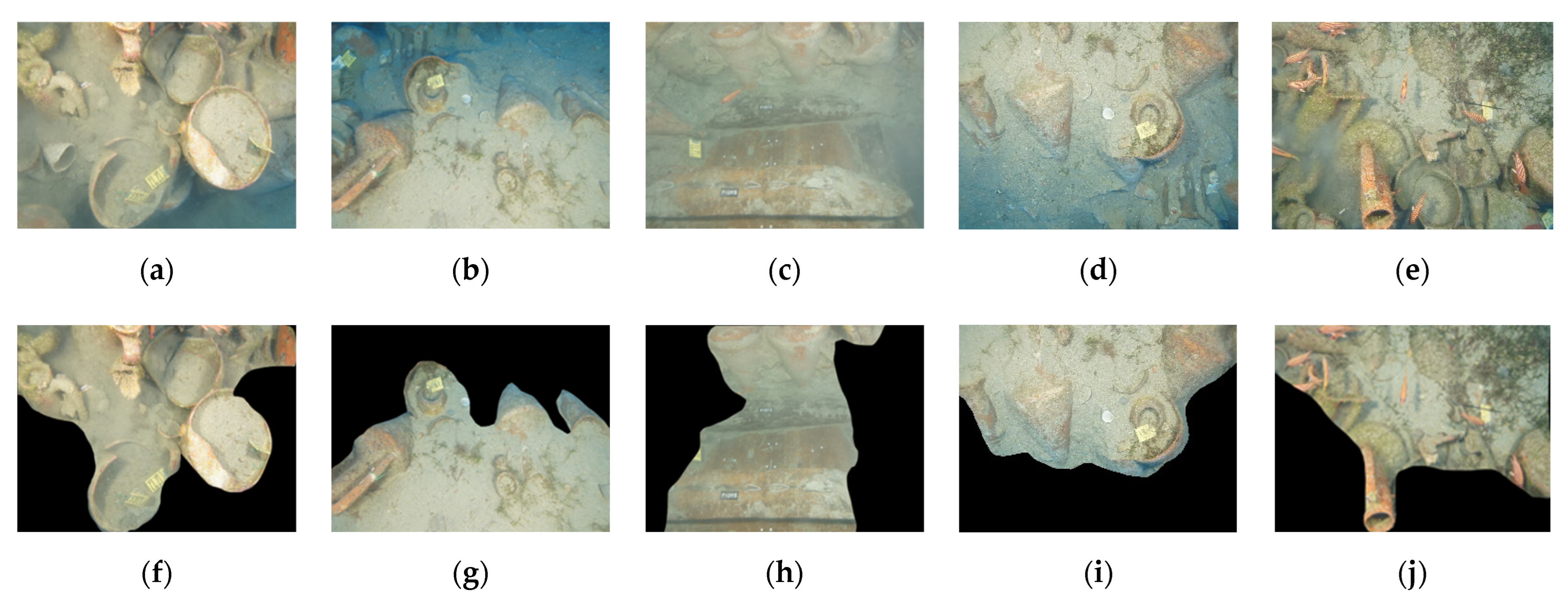
3.1. Dataset Formation

The idea of the following pipeline is to utilize SfM-extracted points from the images and use them to create an appropriate dataset for NN training that will predict the actual colour of the scene. To specify even more, we acquire these points, and for each point, we know in which images it is present, as well as the respective RGB values of the point, along with the Camera-to-Object Distance in each of the images where the point is present. For example, a point might be present in 10 different images, which means that for that point, we have 10 different RGB and Camera-to-Object Distance (CoD) values. The datasets used for the purpose of this paper were captured with a Canon EOS 7D and a Sony SLT-A57 camera, fully equipped with strobes and UW housings.

The first challenge of this task is to identify points that could serve as “ground truth”. Since there are no real ground-truth points underwater, we manually select multiple points as ground truth from well-lit areas of several images and match them with corresponding points in other images of the same dataset. To perform the extraction, manual masks are created in the well-lit areas of certain images based on human interpretation, (in this study, 20–30 images depending on the dataset), as shown in Figure 3.

Having created these masks, we then proceed by extracting all the points that are present in these areas into a separate list. Then, we match every one of those points with its correspondent points in the rest of the image dataset. Now that the ground-truth points with their ground-truth RGB values are separated, the next step is to find the images in which these points have a match. By doing that, we are able to collect, for each point, the image ID, RGB values, and CoD for each image where the point is present. After that, a final list is created for all the points containing all the images where the points are, the different RGB and CoD values for each image where the points are present, and next to them, the unique RGB values for these points. To clarify, let us say that in the final list, we have point number 1, where this point is documented in 10 “uncorrected images” alongside the different RGB and CoD values. For all these 10 different entries, there is only one RGB entry as “ground truth”, which has been extracted from a masked image that also contains the point. In all the datasets that were tested in this study, the final list for each one contained 46,000–139,000 training data. Figure 4 below shows the histograms related to the number of photos to which a ground-truth point was matched.

As shown in Figure 4 above, all GT points were visible and matched to points in at least 3 images. Depending on the dataset, the number of matches for some GT points ranged from 3 to 25 images (left histogram) to 3–13 images (right histogram).

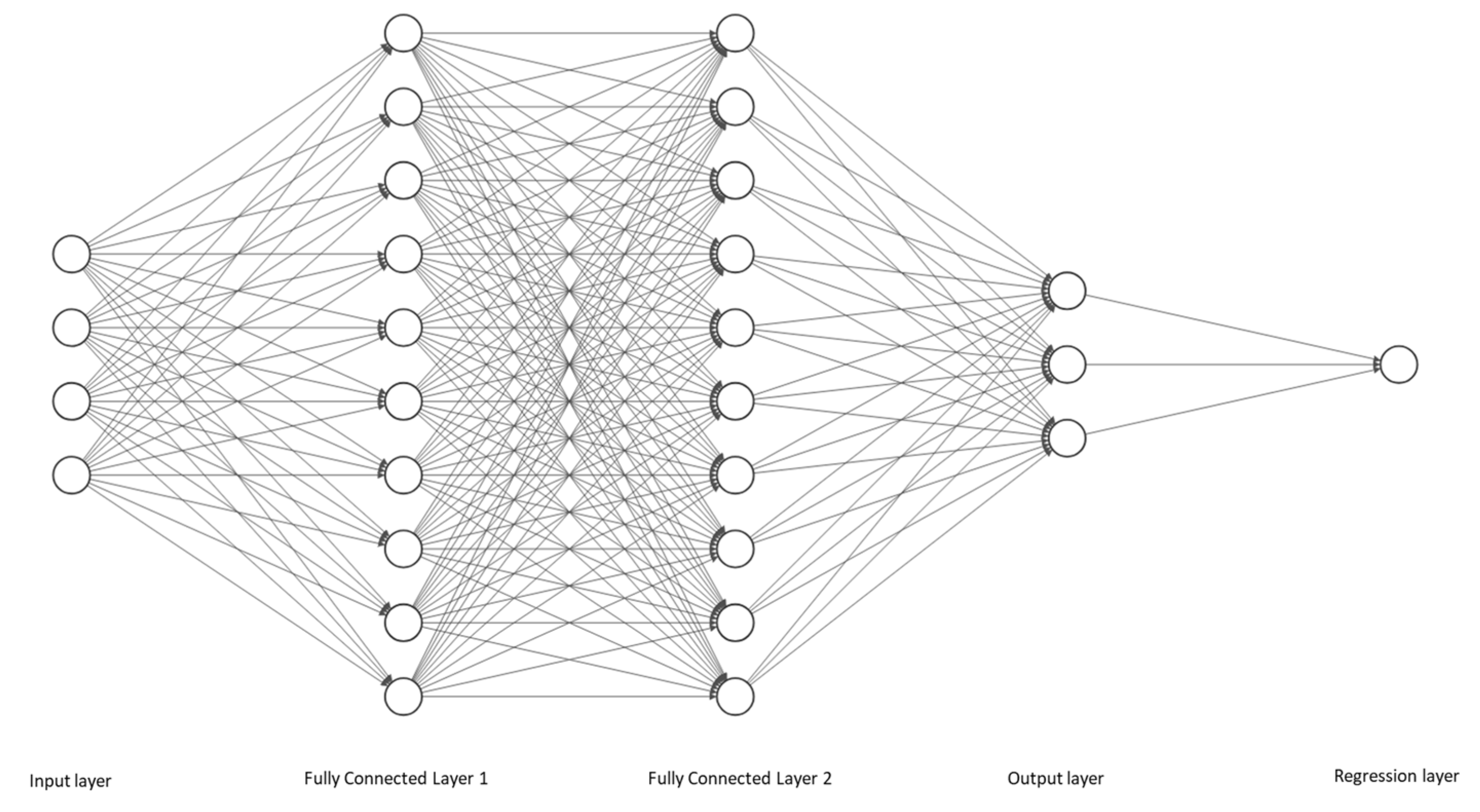
3.2. Network Architecture

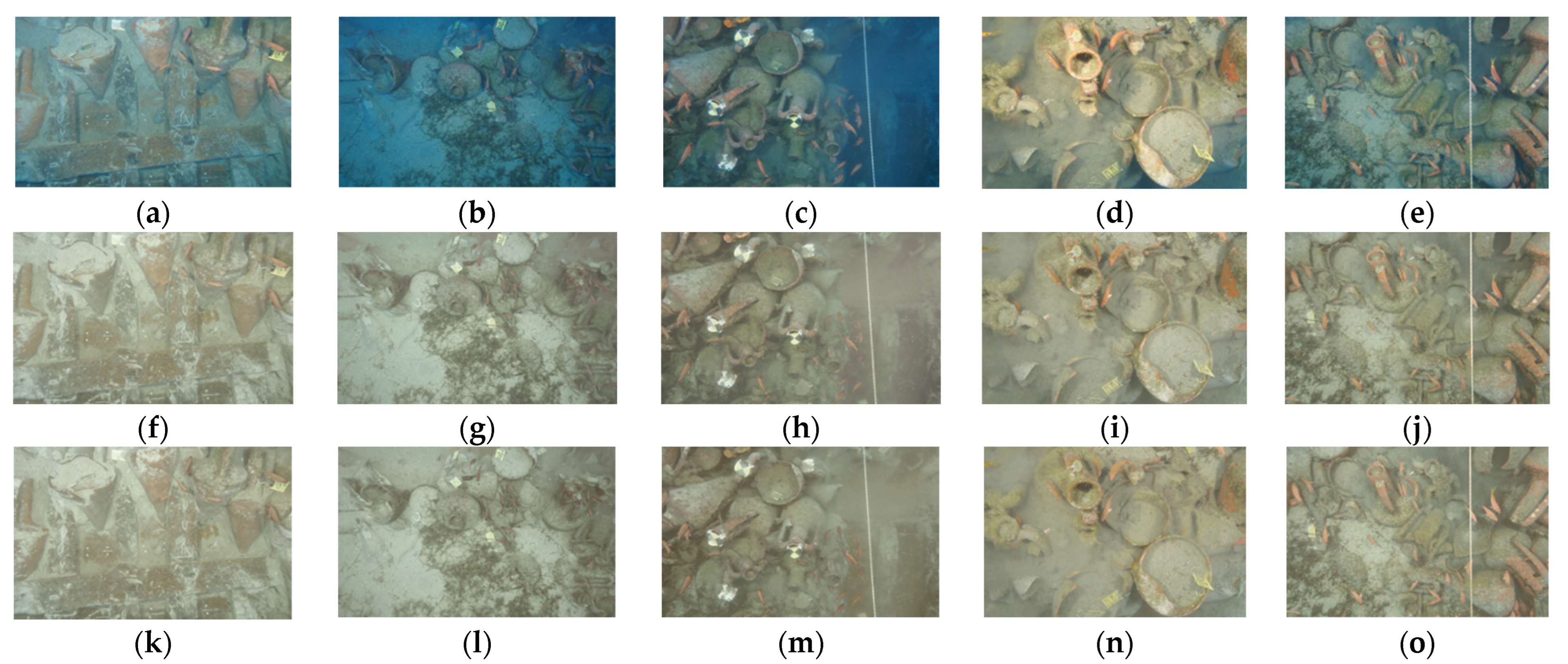
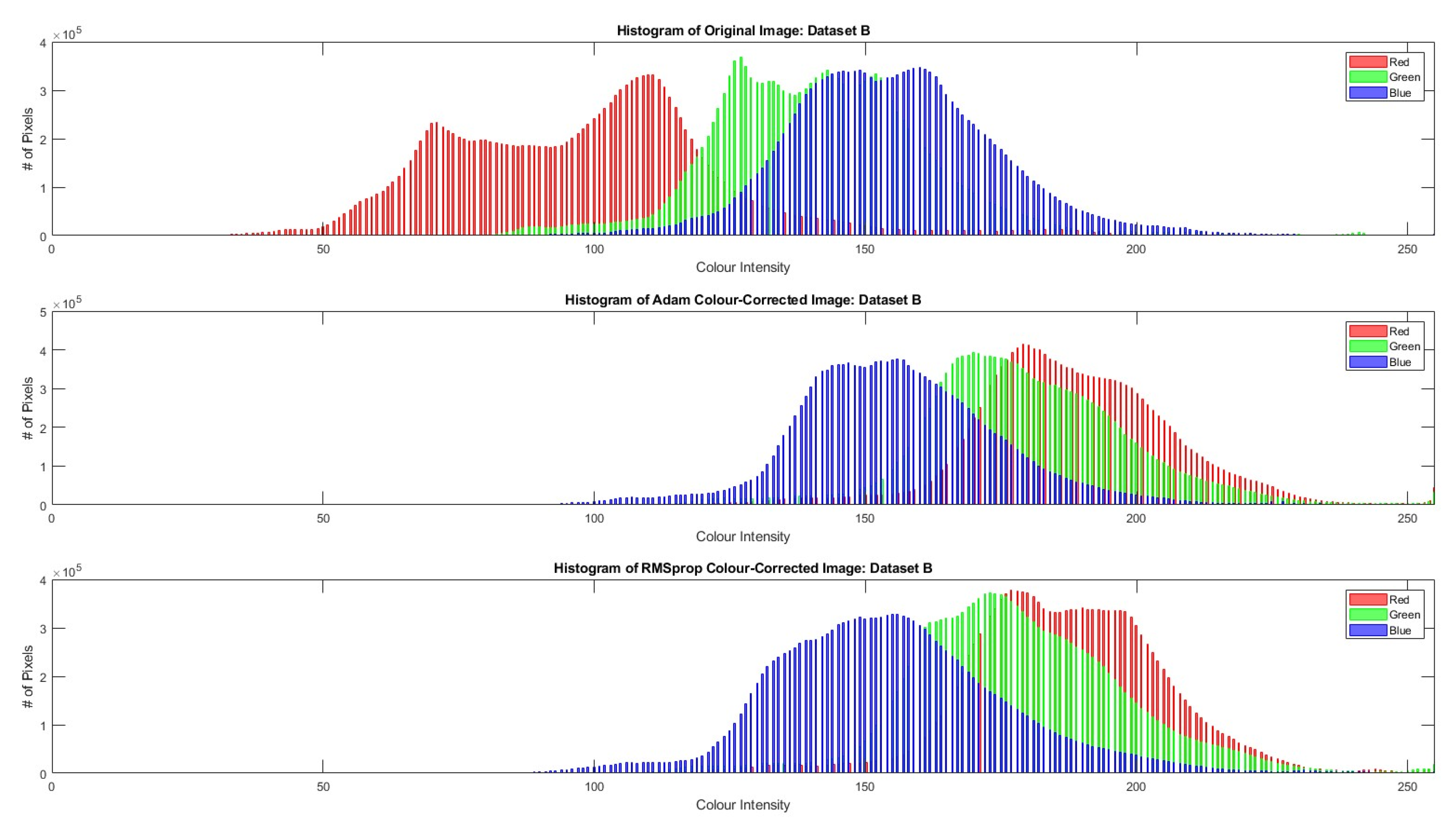
We decided to use a Feedforward Neural Network (FNN) for the purposes of our study because it is a suitable choice for simple data due to several reasons. Firstly, FNNs are straightforward and easy to implement, making them accessible for simple tasks where complex architectures might be unnecessary [53]. Their simplicity facilitates rapid prototyping and experimentation with different network architectures and hyperparameters [54]. Secondly, FNNs excel at learning linear and non-linear relationships between input features and target variables [20]. For simple data with clear patterns or separable classes, FNNs can effectively capture and model these relationships without the need for more complex architectures. Additionally, FNNs are computationally efficient, making them well suited for processing small- to medium-sized datasets commonly encountered in simple-data scenarios [55]. Their efficiency enables faster training times and inference, which is advantageous when dealing with straightforward tasks where computational resources might be limited. Overall, FNNs offer a pragmatic and effective solution for simple data by providing a balance among performance, simplicity, and computational efficiency.

The next step of the proposed methodology is to set up the desired FNN. The code was written in MATLAB, and it executed a very specific pipeline.

First, we split the data into three sets: training, validation, and test sets. The training set (Xtrain and Ytrain) contains the input features (X) and the corresponding target labels (Y) for the first 70% of data. The validation set (Xval and Yval) includes the next 15% of data and the test set (Xtest and Ytest) the remaining 15%.

The network parameters are determined based on several key considerations. Firstly, the number of input neurons (4) corresponds to the dimensionality of the input data (R, G, B, CoD), ensuring that each feature is adequately represented. The inclusion of two hidden layers strikes a balance between capturing complex patterns and avoiding excessive model complexity. Each hidden layer contains 10 neurons, providing flexibility to learn diverse features while maintaining computational efficiency. Rectified Linear Unit (ReLU) activation functions introduce non-linearity, crucial to modelling complex relationships within the data. The output layer comprises 3 neurons, aligning with the classification task’s requirement to predict probabilities for each of the 3 output classes (Rtrue, Gtrue, and Btrue). These parameters collectively aim to optimize model performance by effectively capturing relevant features, managing complexity, and facilitating accurate predictions. Figure 5 shows the network architecture in a simple diagram.

The choice of training options plays a pivotal role in optimizing the network’s learning process and ensuring robust model performance. Firstly, we select the Adam or RMSprop optimization algorithm, which is crucial for efficient gradient descent and convergence to optimal solutions. These algorithms adaptively adjust learning rates based on past gradients, enabling faster convergence and a better handling of sparse gradients in high-dimensional spaces. Secondly, we set a maximum number of training epochs to 100, which strikes a balance between allowing the model to learn complex patterns and preventing overfitting by limiting training time. Additionally, we select a mini-batch size of 64 in order to enhance computational efficiency by processing multiple examples simultaneously, facilitating faster convergence and reducing memory requirements. Furthermore, the training data are shuffled every epoch to prevent the network from memorizing the sequence of data and ensure that diverse examples are presented during training, promoting generalization. Defining the validation data as the split validation set (Xval and Yval) allows for the independent evaluation of the model’s performance during training, facilitating early detection of overfitting and guiding hyperparameter tuning. Lastly, validation is performed every 10 epochs, providing frequent checkpoints for monitoring model performance and adjusting training strategies if necessary, thus promoting stable convergence and preventing divergence. These training options collectively optimize the network’s learning dynamics, enhance generalization, and ensure robust performance on unseen data.

Finally, the neural network is trained by using the defined training options. It passes the training data (Xtrain and Ytrain), the network layers, and the training options as input arguments. The trained network and the training information are returned as output.

After training is complete, the validation and test sets are passed as input to the prediction function, which applies the trained network to the input data and produces predicted output values (Ypred). These predicted values represent the model’s estimation of the target labels for the validation set. After obtaining the predicted values (Ypred) for the validation set, the correlation coefficients between the predicted values (Ypred) and the actual target labels (Yval, Ytest) are calculated. The correlation coefficients measure the linear relationship between the predicted and actual values, ranging from −1 (perfect negative correlation) to 1 (perfect positive correlation). A value close to 1 indicates a strong positive relationship between the predictions and the actual labels.

Here, it must be stated that MATLAB supports a number of training optimisation algorithms, such as SGD, Adam, and RMSprop. Each one has its pros and cons. It is important to note that the choice of optimisation algorithm depends on various factors, including the specific problem, the dataset, the network architecture, and the computational resources available. There may not be a single algorithm that works best for all situations, which is why it is often recommended to experiment with different algorithms and hyperparameters to find the best configuration for a given problem. This is why, for the purpose of this study, we experimented with the 3 abovementioned algorithms. A brief explanation of each of the 3 optimisers is given below.

Stochastic Gradient Descent (SGD): SGD is a widely used optimisation algorithm for training deep neural networks. It works by updating the model parameters in the direction of the negative gradient of the loss function with respect to the parameters. In each iteration, a random batch of training samples is selected to estimate the gradient. The learning rate is a hyperparameter that determines the step size for the parameter updates. One of the main drawbacks of SGD is that it can be slow to converge and may get stuck in local minima [20].

Adaptive Moment Estimation (Adam): Adam is a popular optimisation algorithm that uses a combination of the gradient and the moving average of the past gradients to update the parameters. It adapts the learning rate for each parameter based on the estimates of the first and second moments of the gradients. Adam is known for its ability to converge quickly and works well in practice in a wide range of problems [56].

RMSprop: RMSprop is an optimisation algorithm that uses the moving average of the squared gradients to scale the learning rate for each parameter. It addresses the issue of the diminishing learning rate by using a moving average of the gradients instead of the sum of the squared gradients. It can work well in practice, but it may stop making progress after a certain number of iterations [57].

After experimenting with all 3 optimisers, SGD failed to provide any meaningful results; thus, we decided to not evaluate it further or conduct any more training by using it. After several tests and adjustments, we decided to adopt the Adam and RMSprop optimisers along with the described training parameters for the purpose of our research, since they provided good results regarding training and predictions that we will showcase in the next section.

4. Results

This section will present the training and prediction results obtained by using the Adam and RMSprop optimisers on three different datasets captured in 2018 and 2019 at the Mazotos excavation site. Two datasets from 2019 were captured by using a Sony SLT-A57 camera, and one dataset from 2018 was captured by using a Canon EOS 7D camera. By using these three different datasets captured on different dates with different cameras, hence different conditions, we ensure that the methodology is independent of the camera and environmental conditions.

Table 1. Regression of validation and test data after training by using Adam and RMSprop optimisers.

Dataset	A	B	C
Adam Val R	0.781	0.874	0.799
Adam Test R	0.809	0.821	0.812
RMSprop Val R	0.777	0.821	0.807
RMSprop Test R	0.807	0.751	0.817

below shows the regression on test and validation data after training by using the two optimisers, and

Table 2. Information regarding data acquisition and SfM-MVS-derived results.

Dataset	A	B	C
Camera	Sony SLT-A57	Sony SLT-A57	Canon EOS 7D
Housing	Ikelite (dome)	Ikelite (dome)	Nauticam (dome)
Strobes	Ikelite DS125	Ikelite DS125	Inon Z-240 Type 4
Resolution	4912 × 3264	4912 × 3264	5184 × 3456
Date	23 October 2019	20 October 2019	15 October 2018
Time (EEST)	09:00–09:20	13:12–13:32	12:48–13:08
# of images	307	173	104
# of SfM points	154 k	225 k	180 k
# of GT points	29 k	22 k	22 k
# of training samples	139 k	69 k	46 k
Bundle adjustment RMSE	2.7 cm	2.9 cm	2.6 cm
Min CoD of GT points	0.702 m	0.424 m	0.523 m
Max CoD of GT points	1.327 m	0.883 m	1.171 m
Mean CoD of GT points	1.010 m	0.681 m	0.958 m
Mean Acquisition Distance	1.52 m	1.38 m	1.07 m

shows general information regarding data acquisition and SfM-MVS-derived results.

Based on the quantitative metrics shown in Table 1, the training was considered successful, since the correlation/regression values of validation and test data when compared with the predicted ranged from 0.75 to 0.87, with 1.0 being the absolute best and −1.0 being the absolute worst values that could occur.

Bearing that in mind, we proceeded with predictions on each dataset of images. In other words, we used the uncorrected RGB values and the CoD for each pixel of the image as input, and the algorithm provided a colour-corrected image. Below, in Figure 6, five images from Dataset A are shown alongside with the colour-corrected counterparts obtained by using the predictors from the Adam- and RMSprop-based training.

From the visual inspection of the sample above, it is clear that the algorithm manages to predict and restore the colour of the scene to a satisfying degree. In the example above, we used images from different angles with various elements in the scene. In the first column, we can see that the amphorae’s and wood’s colours are restored quite well, as they resemble the expected ceramics’ and wood’s colours, i.e., red and brown, respectively. The second column shows some of the limitations of the predictor, since the scene is slightly farther away from the camera in this case. This indicates that initially, there were not many similar training data during the training, and it shows the sensitivity and direct correlation between the distance and the colour decay. Another notable observation can be made from the fourth column, where we see that in the original image, the upper centre at the amphorae’s opening is overexposed, but in the restored images, we can see that this overexposure is compensated as well as the colour decay towards the darker edges of the image.

Following the first example, we proceeded with the same pipeline on Dataset B, captured on a different day with the same camera, Sony SLT-A57. In Figure 7, we notice that both the Adam and RMSprop predictors provide very visually realistic results, restoring a large portion of the missing colour information. The main downside in this example is that the corrected images may seem slightly overexposed. This is due to the training samples, more specifically the adopted “ground truth” points from the scene. These points were slightly overexposed due to the close range of the capture, which resulted in slightly overexposed colour-corrected images. This validates the statement that for accurate prediction from training, the ground-truth data are perhaps the biggest key factor.

After evaluating the results on datasets from the same camera, we repeated the same process on a different dataset acquired a year prior, in 2018 (Dataset C), this time by using a different camera, Canon EOS 7D. As shown in Figure 8, both the Adam and RMSprop optimisers provide good training results and predictions for the images. This proves that the proposed methodology is independent of the camera, date, and environmental conditions. Like in the previous example, the result is heavily dependent on the ground truth that was extracted from the dataset itself. The results of this example seem to provide images with a slight white tint, which is due to the training samples. Regardless of the minor downsides, the results from all three datasets are very promising, since the colour of the scene is greatly restored.

In an ideal scenario, we would have liked to quantify the results of the proposed methodology. Unfortunately, that was not possible with the datasets used. A simple but effective way to perform a quantitative evaluation would be the use of colour charts. Since data acquisition was not performed for the purposes of our research but for documentation purposes, that was not feasible at the time. Although we could not quantify the results, we proceeded by evaluating and analysing the colourfulness of the scenery before and after colour restoration. To do so, we extracted the image histograms of several images before and after the predictions by using the Adam and RMSprop optimizers. Below, in Figure 9, Figure 10 and Figure 11, we present the image histograms of one sample image from every dataset before and after image restoration.

As shown above, both optimizers managed to significantly restore the missing information of the red and green colours across the images. We also observed a slight increase in the blue colour inside the scene (Dataset C), which is not noticeable in the visual results shown above in Figure 8. From the image histograms, it is clear that a significant amount of colour information is restored in the colour-corrected images for both optimizers.

A last resort for a quantitative evaluation of our results was the introduction of non-reference evaluation metrics. Three metrics were used: UCIQE [58], UIQM [59], and CCF [60]. UCIQE and UIQM were also utilized in [61].

All three metrics are used to assess the quality of underwater colour images when no real reference data are available. Lower values often indicate better image quality. These values suggest that the image is closer in quality to the reference or ideal standard. Higher values typically suggest poorer image quality. These values indicate that the image deviates more from the reference or ideal standard in terms of quality. The above two statements are true for all three metrics.

Table 3. The results after the implementation of the 3 non-reference evaluation metrics on the original and colour-corrected images.

	UCIQE			UIQM			CCF
Image	Original	Adam	RMSprop	Original	Adam	RMSprop	Original	Adam	RMSprop
A1	0.4995	0.415	0.415	0.4521	0.337	0.3277	11.6494	10.9878	10.7899
A2	0.4525	0.3991	0.3991	0.4935	0.4205	0.4155	14.1839	13.0842	13.086
A3	0.4777	0.3889	0.3889	0.3994	0.340	0.3244	13.5161	10.7012	9.8241
A4	0.4111	0.3585	0.3585	0.4591	0.3943	0.3851	11.2058	10.7861	10.4697
A5	0.429	0.3673	0.3673	0.4241	0.3825	0.3762	12.1364	11.692	11.7376
B1	0.499	0.3983	0.3983	0.3874	0.3057	0.3145	11.3282	9.9403	10.2349
B2	0.5059	0.4207	0.4207	0.5013	0.4055	0.4117	14.8991	13.7815	13.9383
B3	0.4172	0.3523	0.3523	0.3314	0.3143	0.3283	10.0052	9.6501	9.9734
B4	0.4863	0.3745	0.3745	0.4331	0.3803	0.3865	12.8144	12.0295	12.5552
C1	0.4817	0.3412	0.3412	0.5974	0.4694	0.4675	12.9167	11.2434	10.9898
C2	0.569	0.423	0.423	0.6624	0.4964	0.4925	16.5993	14.6705	14.3572
C3	0.5504	0.4355	0.4355	0.6395	0.494	0.5106	19.1362	15.8096	15.6753
C4	0.5382	0.4183	0.4183	0.635	0.4679	0.4754	16.6003	15.9823	15.5284

below shows the obtained metric values of the original images and their colour-corrected counterparts.

Table 3 above shows that the obtained colour-corrected images are improved when compared with the originals, as the metrics suggest, since all the values of the Adam- and RMSprop-derived images are lower than their original counterparts. This shows that in our case, the qualitative and quantitative evaluations agree with each other. Ideally, the use of colour charts would have helped us identify how far from the truth the predicted colours of the scene are, but as we previously mentioned, that was not possible with the used datasets.

5. Discussion

This methodology is an attempt to address the issue of colour attenuation in deep waters in artificial-light scenarios. What we present is an initial attempt to address the problem of severe colour degradation in deep waters using a self-adaptive colour calibration method independent of any physical and environmental parameters with the use of SfM-MVS and FNN techniques. The only requirement is that the geometric setup of camera and lights is stable during acquisition. The dataset must contain some images which are well lit, i.e., close enough to the object, providing adequate “ground-truth” information of the scene’s objects, like sand, amphorae, and wood, in our case. Increased overlapping information among images is desired so that the SfM algorithms can identify and match homologous points across several images. Apart from the actual RGB values, the depth maps that contain the Camera-to-Object Distance for each pixel in the image must be calculated from MVS and used as input for the NN process.

More specifically, the goal, as defined by real-world scenarios, was to restore the colour information from archive datasets acquired with strobe-mounted cameras without the presence of natural light. Usually, such datasets lack necessary environmental information, as well as spectral information, to describe a full analytical attenuation model to restore colour. The motivation was to develop a pipeline that manages to restore colour without any environmental information. The method is designed for the following conditions: lack of information regarding the whole setup, that is, the positioning of the strobes relative to the camera; lack of information about the environmental conditions; as it occurs in many cases, lack of information about the camera itself; and no actual ground-truth information underwater. Thus, we propose a pipeline which utilises the dataset itself and, more specifically, the areas with sufficient lighting in order to train an NN optimiser like Adam and RMSprop for the prediction of the true colours of the UW scenery.

An added advantage of this approach is that archived datasets captured for SfM-MVS 3D reconstruction can be utilised. The only real constraint is that the dataset must have been captured by a rigid camera–strobe rig, i.e., no change in camera projection centre and pose of the strobe or strobes used should have occurred.

This would not have been possible without the use of Structure from Motion techniques, because through that we are able to match the extracted “ground-truth” points with their homologous points in other images where the colour is decayed; thus, we can create a dataset suitable for training by using NNs such as the one described in this paper. These techniques have led us to explore the possibility of colour restoration of archive datasets with a lack of crucial information. The results presented are promising, as the proposed methodology can be applied to different datasets acquired under different conditions with different cameras.

The main shortcoming of this work is the lack of a reference-based quantitative evaluation. The correlation coefficients provided after the training are quantitative indicators regarding the training itself. The non-reference metrics used on the colour-corrected images allowed for the best quantitative evaluation we could have, since the data were only acquired for site documentation purposes. This means that the inclusion of colour charts, which can be photographed on land and then placed on the scene, was deemed unnecessary and time-consuming at the time. With that option, we could have compared the colour values of the colour patches on the colour-corrected images with the colour values captured on land for reference-based quantitative evaluation. This could be the subject of our future work, which can help us further support the legitimacy of our method. Another topic that we would like to address in the future is the automation of “ground-truth” point selection.

References

1. Klemen, I. Underwater Image-Based 3D Reconstruction with Quality Estimation; University of Girona: Girona, Spain, 2021. [Google Scholar]
2. Wang, Y.; Song, W.; Fortino, G.; Qi, L.Z.; Zhang, W.; Liotta, A. An Experimental-Based Review of Image Enhancement and Image Restoration Methods for Underwater Imaging. IEEE Access 2019, 7, 140233–140251. [Google Scholar] [CrossRef]
3. Bekerman, Y.; Avidan, S.; Treibitz, T. Unveiling Optical Properties in Underwater Images. In Proceedings of the 2020 IEEE International Conference on Computational Photography (ICCP), St. Louis, MO, USA, 24–26 April 2020; pp. 1–12. [Google Scholar] [CrossRef]
4. Morel, A.; Gentili, B.; Claustre, H.; Babin, M.; Bricaud, A.; Ras, J.; Tièche, F. Opticals Properties of the “Clearest” Natural Waters. Limnol. Oceanogr. 2007, 52, 217–229. [Google Scholar] [CrossRef]
5. Menna, F.; Agrafiotis, P.; Georgopoulos, A. State of the Art and Applications in Archaeological Underwater 3D Recording and Mapping. J. Cult. Herit. 2018, 33, 231–248. [Google Scholar] [CrossRef]
6. Jerlov, N.G.; Koczy, F.F.; Schooner, A. Photographic Measurements of Daylight in Deep Water; Reports of the Swedish Deep-Sea Expedition, 1947–1948 ; v. 3: Physics and Chemistry; Elanders Boktr: Mölnlycke, Sweden, 1951. [Google Scholar]
7. Solonenko, M.G.; Mobley, C.D. Inherent Optical Properties of Jerlov Water Types. Appl. Opt. 2015, 54, 5392. [Google Scholar] [CrossRef] [PubMed]
8. Akkaynak, D.; Treibitz, T.; Shlesinger, T.; Tamir, R.; Loya, Y.; Iluz, D. What Is the Space of Attenuation Coefficients in Underwater Computer Vision? Proceedings of thr 30th IEEE Conference on Computer Vision and Pattern Recognition, CVPR 2017, Honolulu, HI, USA, 21–26 July 2017; pp. 568–577. [Google Scholar] [CrossRef]
9. Blasinski, H.; Breneman IV, J.; Farrell, J. A model for estimating spectral properties of water from rgb images. In Proceedings of the International Conference on Image Processing (ICIP), Paris, France, 27–30 October 2014; pp. 610–614. [Google Scholar]
10. Lebart, K.; Smith, C.; Trucco, E.; Lane, D.M. Automatic Indexing of Underwater Survey Video: Algorithm and Benchmarking Method. IEEE J. Ocean. Eng. 2003, 28, 673–686. [Google Scholar] [CrossRef]
11. Yuh, J.; West, M. Underwater Robotics; Taylor & Francis: Oxfordshire, UK, 2001; Volume 15, ISBN 1568553013. [Google Scholar]
12. Chao, L.; Wang, M. Removal of Water Scattering. In Proceedings of the ICCET 2010—2010 International Conference on Computer Engineering and Technology, Proceedings, Chengdu, China, 16–18 April 2010; Volume 2, pp. 35–39. [Google Scholar] [CrossRef]
13. Hou, W.; Gray, D.J.; Weidemann, A.D.; Fournier, G.R.; Forand, J.L. Automated Underwater Image Restoration and Retrieval of Related Optical Properties. In Proceedings of the IEEE International Geoscience & Remote Sensing Symposium, IGARSS 2007, Barcelona, Spain, 23–28 July 2007; pp. 1889–1892. [Google Scholar] [CrossRef]
14. Schechner, Y.Y.; Karpel, N. Recovery of Underwater Visibility and Structure by Polarization Analysis. IEEE J. Ocean. Eng. 2005, 30, 570–587. [Google Scholar] [CrossRef]
15. Murphy, K.P. Machine Learning: A Probabilistic Perspective; MIT Press: Cambridge, MA, USA, 2013; ISBN 9780262018029 0262018020. [Google Scholar]
16. Pyle, D. Data Preparation for Data Mining; The Morgan Kaufmann Series in Data Management Systems; Elsevier Science: Amsterdam, The Netherlands, 1999; ISBN 9781558605299. [Google Scholar]
17. Hastie, T.; Tibshirani, R.; Friedman, J. The Elements of Statistical Learning; Springer Series in Statistics; Springer New York Inc.: New York, NY, USA, 2001. [Google Scholar]
18. Jordan, M.I.; Mitchell, T.M. Machine Learning: Trends, Perspectives, and Prospects. Science 2015, 349, 255–260. [Google Scholar] [CrossRef] [PubMed]
19. Aggarwal, C.C. Teaching Deep Learners to Generalize; Springer: Cham, Switzerland, 2018; ISBN 9783319944623. [Google Scholar]
20. Goodfellow, I.; Bengio, Y.; Courville, A. Deep Learning; MIT Press: Cambridge, MA, USA, 2016. [Google Scholar]
21. Russell, S.; Norvig, P. Artificial Intelligence: A Modern Approach, 3rd ed.; Prentice Hall: Hoboken, NJ, USA, 2010. [Google Scholar]
22. Krizhevsky, A.; Sutskever, I.; Hinton, G.E. ImageNet Classification with Deep Convolutional Neural Networks. In Proceedings of the Advances in Neural Information Processing Systems; Pereira, F., Burges, C.J., Bottou, L., Weinberger, K.Q., Eds.; Curran Associates, Inc.: Red Hook, NY, USA, 2012; Volume 25. [Google Scholar]
23. Isola, P.; Zhu, J.Y.; Zhou, T.; Efros, A.A. Image-to-Image Translation with Conditional Adversarial Networks. In Proceedings of the Proceedings—30th IEEE Conference on Computer Vision and Pattern Recognition, CVPR 2017, Honolulu, HI, USA, 21–26 July 2017; pp. 5967–5976. [Google Scholar] [CrossRef]
24. Goodfellow, I.; Pouget-Abadie, J.; Mirza, M.; Xu, B.; Warde-Farley, D.; Ozair, S.; Courville, A.; Bengio, Y. Generative Adversarial Nets. In Proceedings of the Advances in Neural Information Processing Systems; Ghahramani, Z., Welling, M., Cortes, C., Lawrence, N., Weinberger, K.Q., Eds.; Curran Associates, Inc.: Red Hook, NY, USA, 2014; Volume 27. [Google Scholar]
25. Ledig, C.; Theis, L.; Huszár, F.; Caballero, J.; Cunningham, A.; Acosta, A.; Aitken, A.; Tejani, A.; Totz, J.; Wang, Z.; et al. Photo-Realistic Single Image Super-Resolution Using a Generative Adversarial Network. In Proceedings of the Proceedings—30th IEEE Conference on Computer Vision and Pattern Recognition, CVPR 2017, Honolulu, HI, USA, 21–26 July 2017; pp. 105–114. [Google Scholar] [CrossRef]
26. Ren, S.; He, K.; Girshick, R.; Sun, J. Faster R-CNN: Towards Real-Time Object Detection with Region Proposal Networks. IEEE Trans. Pattern. Anal. Mach. Intell. 2017, 39, 1137–1149. [Google Scholar] [CrossRef] [PubMed]
27. Akkaynak, D.; Treibitz, T. A Revised Underwater Image Formation Model. In Proceedings of the IEEE Computer Society Conference on Computer Vision and Pattern Recognition, Salt Lake City, UT, USA, 18–22 June 2018; pp. 6723–6732. [Google Scholar] [CrossRef]
28. Akkaynak, D.; Treibitz, T. Sea-THRU: A Method for Removing Water from Underwater Images. In Proceedings of the IEEE Computer Society Conference on Computer Vision and Pattern Recognition 2019, Long Beach, CA, USA, 15–20 June 2019; pp. 1682–1691. [Google Scholar] [CrossRef]
29. Bryson, M.; Johnson-Roberson, M.; Pizarro, O.; Williams, S.B. Colour-Consistent Structure-from-Motion Models Using Underwater Imagery. Robot. Sci. Syst. 2013, 8, 33–40. [Google Scholar] [CrossRef]
30. Bryson, M.; Johnson-Roberson, M.; Pizarro, O.; Williams, S.B. True Color Correction of Autonomous Underwater Vehicle Imagery. J. Field Robot. 2016, 33, 853–874. [Google Scholar] [CrossRef]
31. Demesticha, S. The 4th-Century-BC Mazotos Shipwreck, Cyprus: A Preliminary Report. Int. J. Naut. Archaeol. 2011, 40, 39–59. [Google Scholar] [CrossRef]
32. Demesticha, S.; Skarlatos, D.; Neophytou, A. The 4th-Century B.C. Shipwreck at Mazotos, Cyprus: New Techniques and Methodologies in the 3D Mapping of Shipwreck Excavations. J. Field Archaeol. 2014, 39, 134–150. [Google Scholar] [CrossRef]
33. Corchs, S.; Schettini, R. Underwater Image Processing: State of the Art of Restoration and Image Enhancement Methods. EURASIP J. Adv. Signal Process. 2010, 2010, 1–14. [Google Scholar] [CrossRef]
34. Vlachos, M.; Skarlatos, D. An Extensive Literature Review on Underwater Image Colour Correction. Sensors 2021, 21, 5690. [Google Scholar] [CrossRef]
35. Ancuti, C.; Ancuti, C.O.; Haber, T.; Bekaert, P. Enhancing Underwater Images and Videos by Fusion. In Proceedings of the IEEE Computer Society Conference on Computer Vision and Pattern Recognition 2012, Providence, RI, USA, 16–21 June 2012; pp. 81–88. [Google Scholar] [CrossRef]
36. Bianco, G.; Muzzupappa, M.; Bruno, F.; Garcia, R.; Neumann, L. A New Color Correction Method for Underwater Imaging. Int. Arch. Photogramm. Remote Sens. Spat. Inf. Sci.—ISPRS Arch. 2015, 40, 25–32. [Google Scholar] [CrossRef]
37. Nurtantio Andono, P.; Eddy Purnama, I.K.; Hariadi, M. Underwater Image Enhancement Using Adaptive Filtering for Enhanced Sift-Based Image Matching. J. Theor. Appl. Inf. Technol. 2013, 52, 273–280. [Google Scholar]
38. Ancuti, C.O.; Ancuti, C.; De Vleeschouwer, C.; Neumann, L.; Garcia, R. Color Transfer for Underwater Dehazing and Depth Estimation. In Proceedings of the Proceedings—International Conference on Image Processing, ICIP 2018, Athens, Greece, 7–10 October 2018; pp. 695–699. [Google Scholar] [CrossRef]
39. Zhao, X.; Jin, T.; Qu, S. Deriving Inherent Optical Properties from Background Color and Underwater Image Enhancement. Ocean Eng. 2015, 94, 163–172. [Google Scholar] [CrossRef]
40. Yan-Tsung, P.; Xiangyun, Z.; Pamela, C. Single underwater image enhancement using depth estimation based on blurriness. In Proceedings of the 2015 IEEE International Conference on Image Processing (ICIP), Quebec City, QC, Canada, 28 September 2015; pp. 2–6. [Google Scholar]
41. Torres-Méndez, L.A.; Dudek, G. Color Correction of Underwater Images for Aquatic Robot Inspection; Springer: Berlin/Heidelberg, Germany, 2005; pp. 60–73. [Google Scholar] [CrossRef]
42. Li, C.; Guo, J.; Guo, C. Emerging from Water: Underwater Image Color Correction Based on Weakly Supervised Color Transfer. IEEE Signal Process Lett 2018, 25, 323–327. [Google Scholar] [CrossRef]
43. Hashisho, Y.; Albadawi, M.; Krause, T.; von Lukas, U.F. Underwater Color Restoration Using U-Net Denoising Autoencoder; IEEE: Piscataway, NJ, USA, 2019. [Google Scholar]
44. Awan, H.S.A.; Mahmood, M.T. Underwater Image Restoration through Color Correction and UW-Net. Electronics 2024, 13, 199. [Google Scholar] [CrossRef]
45. Ertan, Z.; Korkut, B.; Gördük, G.; Kulavuz, B.; Bakırman, T.; Bayram, B. Enhancement of underwater images with artificial intelligence. Int. Arch. Photogramm. Remote Sens. Spat. Inf. Sci. 2024, XLVIII-4/W9-2024, 149–156. [Google Scholar] [CrossRef]
46. Zhu, J.Y.; Park, T.; Isola, P.; Efros, A.A. Unpaired Image-to-Image Translation Using Cycle-Consistent Adversarial Networks. In Proceedings of the IEEE International Conference on Computer Vision 2017, Venice, Italy, 22–29 October 2017; pp. 2242–2251. [Google Scholar] [CrossRef]
47. Lu, J.; Li, N.; Zhang, S.; Yu, Z.; Zheng, H.; Zheng, B. Multi-Scale Adversarial Network for Underwater Image Restoration. Opt. Laser Technol. 2019, 110, 105–113. [Google Scholar] [CrossRef]
48. Li, J.; Skinner, K.A.; Eustice, R.M.; Johnson-Roberson, M. WaterGAN: Unsupervised Generative Network to Enable Real-Time Color Correction of Monocular Underwater Images. IEEE Robot. Autom. Lett. 2018, 3, 387–394. [Google Scholar] [CrossRef]
49. Wang, N.; Zhou, Y.; Han, F.; Zhu, H.; Zheng, Y. UWGAN: Underwater GAN for Real-World Underwater Color Restoration and Dehazing. arXiv 2019, arXiv:1912.10269v2. [Google Scholar]
50. Fabbri, C.; Islam, M.J.; Sattar, J. Enhancing Underwater Imagery Using Generative Adversarial Networks. Proc. IEEE Int. Conf. Robot Autom. 2018, 7159–7165. [Google Scholar] [CrossRef]
51. Gulrajani, I.; Ahmed, F.; Arjovsky, M.; Dumoulin, V.; Courville, A. Improved Training of Wasserstein GANs. arXiv 2017, arXiv:1704.00028. [Google Scholar]
52. Mu, D.; Li, H.; Liu, H.; Dong, L.; Zhang, G. Underwater Image Enhancement Using a Mixed Generative Adversarial Network. IET Image Process. 2023, 17, 1149–1160. [Google Scholar] [CrossRef]
53. Aggarwal, C.C. Neural Networks and Deep Learning; Springer International Publishing: Cham, Switzerland, 2018. [Google Scholar]
54. Müller, A.C.; Guido, S. Introduction to Machine Learning with Python a Guide for Data Scientists Introduction to Machine Learning with Python; O’Reilly Media, Inc.: Sebastopol, CA, USA, 2016. [Google Scholar]
55. Géron, A. Hands-on Machine Learning with Scikit-Learn, Keras, and TensorFlow Concepts, Tools, and Techniques to Build Intelligent Systems, 2nd ed.; O’Reilly Media, Inc.: Sebastopol, CA, USA, 2019. [Google Scholar]
56. Kingma, D.P.; Ba, J.L. Adam: A Method for Stochastic Optimization. In Proceedings of the 3rd International Conference on Learning Representations, ICLR 2015—Conference Track Proceedings, San Diego, CA, USA, 7–9 May 2015; pp. 1–15. [Google Scholar]
57. Hinton, G.E.; Srivastava, N.; Krizhevsky, A.; Sutskever, I.; Salakhutdinov, R.R. Improving Neural Networks by Preventing Co-Adaptation of Feature Detectors. arXiv 2012, arXiv:1207.0580. [Google Scholar]
58. Yang, M.; Sowmya, A. An Underwater Color Image Quality Evaluation Metric. IEEE Trans. Image Process. 2015, 24, 6062–6071. [Google Scholar] [CrossRef]
59. Panetta, K.; Gao, C.; Agaian, S. Human-Visual-System-Inspired Underwater Image Quality Measures. IEEE J. Ocean. Eng. 2016, 41, 541–551. [Google Scholar] [CrossRef]
60. Wang, Y.; Li, N.; Li, Z.; Gu, Z.; Zheng, H.; Zheng, B.; Sun, M. An Imaging-Inspired No-Reference Underwater Color Image Quality Assessment Metric. Comput. Electr. Eng. 2018, 70, 904–913. [Google Scholar] [CrossRef]
61. Li, C.; Guo, C.; Ren, W.; Cong, R.; Hou, J.; Kwong, S.; Tao, D. An Underwater Image Enhancement Benchmark Dataset and Beyond. IEEE Trans. Image Process. 2020, 29, 4376–4389. [Google Scholar] [CrossRef]
Figure 1. A typical case of an underwater image captured by a camera with strobes.
Remotesensing 16 01279 g001
Figure 2. Location of Mazotos shipwreck site. (A. Agapiou, © University of Cyprus, Archaeological Research Unit (ARU). Data compiled from the Geological Survey of Cyprus). Image from [31].
Remotesensing 16 01279 g002
Figure 3. Samples of “ground truth” as manually extracted from selected images of Dataset A. Original images (ae) with the masked “ground-truth” counterparts (fj). Credits: MARELab, © University of Cyprus. Photographer: Massimiliano Secci.
Remotesensing 16 01279 g003
Figure 4. Histograms of the number of images to which the ground-truth points were matched. Datasets (AC).
Remotesensing 16 01279 g004
Figure 5. Network architecture of FNN used for training.
Remotesensing 16 01279 g005
Figure 6. Training results on 5 images with Adam and RMSprop optimisers ((ae) Original images, (fj) Adam optimiser-based prediction results, and (ko) RMSprop optimiser-based prediction results). Dataset A, Camera: Sony SLT-A57. Images acquired at the Mazotos shipwreck site. Credits: MARELab, © University of Cyprus. Photographer: Massimiliano Secci.
Remotesensing 16 01279 g006
Figure 7. Training results on 4 images with Adam and RMSprop optimisers ((ad) Original images, (eh) Adam optimiser-based prediction results, and (il) RMSprop optimiser-based prediction results). Dataset B, Camera: Sony SLT-A57. Images acquired at the Mazotos shipwreck site. Credits: MARELab, © University of Cyprus. Photographer: Massimiliano Secci.
Remotesensing 16 01279 g007
Figure 8. Training results on 4 images with Adam and RMSprop optimisers ((ad) Original images, (eh) Adam optimiser-based prediction results, and (il) RMSprop optimiser-based prediction results). Dataset C, Camera: Canon EOS 7D. Images acquired at the Mazotos shipwreck site. Credits: MARELab, © University of Cyprus. Photographer: Andreas C. Kritiotis.
Remotesensing 16 01279 g008
Figure 9. Image histograms of a sample image from Dataset A. Top: original image; middle: Adam optimizer; bottom: RMSprop optimizer.
Remotesensing 16 01279 g009
Figure 10. Image histograms of a sample image from Dataset B. Top: original image; middle: Adam optimizer; bottom: RMSprop optimizer.
Remotesensing 16 01279 g010
Figure 11. Image histograms of a sample image from Dataset C. Top: original image; middle: Adam optimizer; bottom: RMSprop optimizer.
Remotesensing 16 01279 g011