Abstract
Remote sensing-based models usually have difficulty in generating spatio-temporally continuous terrestrial evapotranspiration (ET) due to cloud cover and model failures. To overcome this problem, machine learning methods have been widely used to reconstruct ET. Therefore, studies comparing and evaluating the accuracy and effectiveness of reconstruction among different machine learning methods at the basin scale are necessary. In this study, four popular machine learning methods, including deep forest (DF), deep neural network (DNN), random forest (RF) and extreme gradient boosting (XGB), were used to reconstruct the ET product, addressing gaps resulting from cloud cover and model failure. The ET reconstructed by the four methods was evaluated and compared for Heihe River Basin. The results showed that the four methods performed well for Heihe River Basin, but the RF method was particularly robust. It not only performed well compared with ground measurements (R = 0.73) but also demonstrated the ability to fully reconstruct gaps generated by the TSEB model across the entire basin. Validation based on ground measurements showed that the DNN and XGB models performed well (R > 0.70). However, some gaps still existed in the desert after reconstruction using the DNN and XGB models, especially for the XGB model. The DF model filled these gaps throughout the basin, but this model had lower consistency compared with ground measurements (R = 0.66) and yielded many low values. The results of this study suggest that machine learning methods have considerable potential in the reconstruction of ET at the basin scale.
1. Introduction
Terrestrial evapotranspiration (ET) is a crucial component of land–atmosphere hydrology, energy and material cycles [1,2]. The accurate and reliable estimation of regional ET is important for basin hydrology, agricultural water management and drought monitoring [3]. Currently, ground measurement systems including the eddy covariance (EC) system and the large-aperture scintillometer (LAS) are commonly used to measure ET under different vegetation types [4,5]. These measurement techniques, however, can only provide valid measurements at a several meters to ~100 m scale, with difficulty in obtaining valid measurements at larger scales [4]. Therefore, ground-based observations are usually used to validate ET products based on remote sensing. By contrast, remote sensing techniques provide the ability to easily monitor large-scale geographical information according to satellites and thus have become a commonly used way of detecting ET.
However, remote sensing techniques can only detect surface parameters related to ET, rather than directly observing ET. In order to acquire reliable ET over larger scales, many remote sensing-based ET simulation models have been proposed that can be used to acquire ET over larger scales [6,7,8,9,10,11,12,13]. Among these models, thermal–infrared-based models are widely used to estimate regional ET based on thermal–infrared-based land surface temperature (LST) [14,15,16]. The two-source energy balance (TSEB) model is one of the most widely applied and has a more reasonable physical mechanism compared to single-source models [6]. It has been shown that the TSEB model can more accurately simulate energy exchanges between the atmosphere, soil and vegetation and is more adaptable to different vegetation types and climatic regions [17,18,19]. The input parameters of the TSEB model include surface boundary parameters based on remote sensing and meteorological parameters [6]. Meteorological reanalysis data overcome the spatial limitations of the observed meteorological data recorded by traditional weather stations and can be employed to drive the TSEB model at large scales [20,21]. However, the TSEB model also relies on inputting thermal–infrared-based surface temperature as a boundary constraint. This often leads to model invalidation in regions where surface temperatures are influenced by solid clouds, thus limiting the practical applications of this model [12,22,23,24]. Moreover, due to the mechanism of the TSEB model, it may still produce gaps in areas shrouded by solid clouds with low radiation, even when land surface temperatures are available [25].
Hence, exploring reliable methods for the spatio-temporal reconstruction of TSEB-estimated ET is significant for agricultural water management and hydrological applications [22,25]. In response to these challenges, various machine learning methods, such as random forest (RF) [26], deep forest (DF) [27], deep neural networks (DNNs) [25] and extreme gradient boosting (XGBoost) [28], have provided viable solutions for the reconstruction of ET. These methods have been applied to estimate or reconstruct the surface parameters from remote sensing data in previous studies [29,30,31,32,33]. The conventional approach usually entails the initial training of a model at the site scale and then expanding the model to a larger regional scale using remote sensing and other data [34,35,36]. However, although such well-trained models typically perform well at the site scale, unevenly distributed and limited sites cannot adequately represent heterogeneous surfaces [35]. Hence, some relevant research has used the effective target parameters obtained from the model as input samples for training machine learning methods, which are used to fill the gaps in the model estimation by combining the spatio-temporal continuous impact factors [25,33]. This innovative methodology ensures that machine learning methods not only fill in the gaps but also guarantee the accuracy and reliability of the models. However, few studies have used this way of reconstructing ET. Whether different machine learning methods perform differently when combined with physical models also needs to be investigated.
The objective of this paper was to generate spatio-temporally continuous daily ET, overcoming the spatial limitations of traditional ground measurement systems and the temporal constraints associated with remote sensing models. To achieve this, four machine learning methods were employed to reconstruct the gaps generated by the TSEB model for Heihe River Basin. In the following sections, we delve into the methodology of combining the TSEB model with machine learning for ET estimation and reconstruction and comprehensively compare the accuracy and effectiveness of the different machine learning methods coupled with the TSEB model at different spatial scales.
2. Materials and Methods
2.1. Study Area and EC Sites
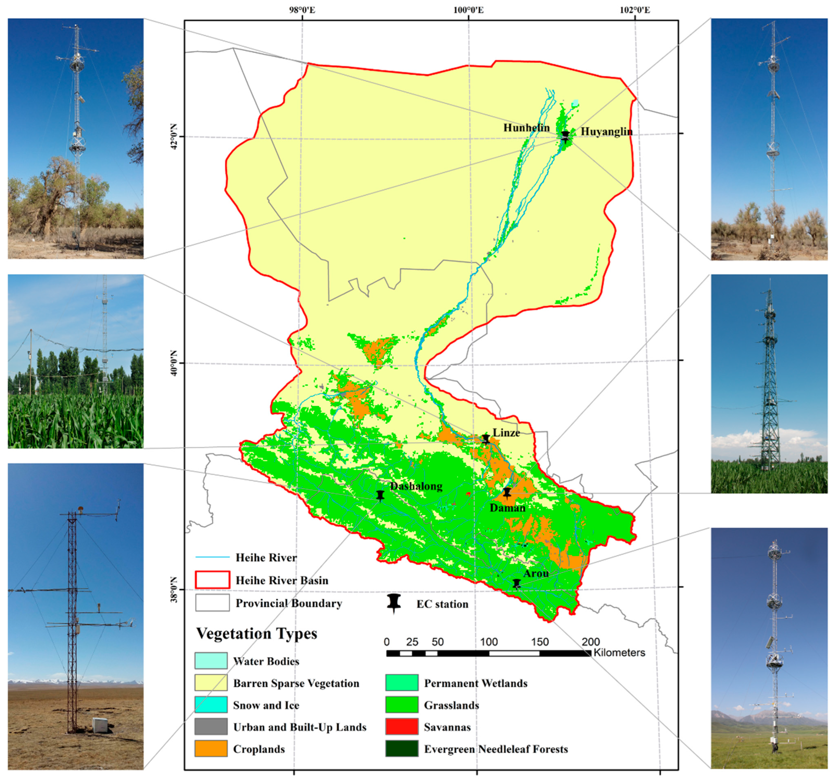
The study area was Heihe River Basin located in the middle of the Hexi corridor, which is the second largest inland basin in northwest China, covering approximately 1,432,000 km2 [37,38]. According to the hydrological characteristics, the basin can be divided into upstream, midstream and downstream sections. Heihe River Basin is characterized by widespread desert, sporadic grassland and cropland, with riparian forest in the downstream regions and widespread grassland, riparian ecosystems, wetland and cropland (cultivated by crops such as maize, wheat and vegetables) in the upstream and midstream regions (Figure 1) [37,38]. This area is in arid and semi-arid regions and has a typical temperate continental climate, with a mean annual temperature of 6.0~8.0 °C, mean annual precipitation of 100~250 mm, and mean annual evapotranspiration of 1200~1800 mm.
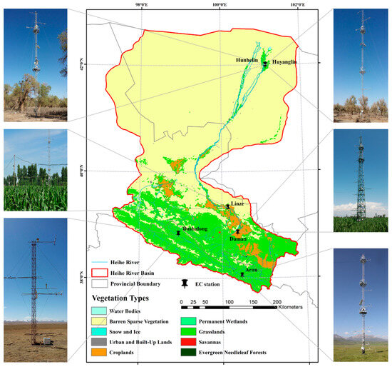
Figure 1.
Study area and vegetation type map for Heihe River Basin and the location of EC sites in the upstream, midstream and downstream regions, along with the landscape around the EC sites.
Heihe Watershed Allied Telemetry Experimental Research (HiWATER) has been conducted in this area to better understand hydrological, ecological and other land surface processes, accumulating numerous surface observation data for this purpose [38]. Six EC stations from 2011 to 2016 with relatively homogeneous surfaces were selected to validate the accuracy of the estimated and reconstructed daily ET in this study (Table 1). These sites include one wetland EC station (Dashalong) [39], one grassland EC station (Arou) [39], two cropland EC stations (Daman and Linze) [5,39,40] and two forest EC stations (Huyanglin and Hunhelin) (Figure 1) [39].

Table 1.
Information on the EC measurement stations. MF (mixed forest), DBF (deciduous broadleaved forest), GRA (grassland), CRO (cropland).
Original EC measurement data were stored as the average latent heat flux per 30 min (48 data per day). In this study, the daily ET measurements were aggregated from 8:00 to 19:00, when less than 25% of the observations were absent. All ground measurement data can be acquired from the National Tibetan Plateau Data Center (TPDC) at https://data.tpdc.ac.cn (accessed on 10 November 2023).
2.2. Multisource Data
In this study, surface boundary parameters for constrained surface heat fluxes, including LST, leaf area index (LAI) and land cover type (LC), needed to be input into the TSEB model. These parameters can be acquired through remote sensing techniques. Among them, the LST dataset utilized a fusion product that combines the Global Land Data Assimilation System (GLDAS) and Terra MODIS LST [41]. This fusion product is based on the time series decomposition model of LST, reconstructing the gaps in MODIS LST, with spatial and temporal resolutions of 1 km and daily [41]. The LAI dataset was collected from the Global Land Surface Satellite (GLASS) LAI dataset with spatial and temporal resolutions of 500 m and 8-day [42]. In order to ensure consistency with other data in the temporal resolution, the LAI was temporally linearly smoothed to a daily scale. The Albedo dataset, which was used for the reconstruction of daily ET, was also collected from GLASS and similarly processed. The land cover type map based on the International Geosphere-Biosphere Programme (IGBP) classification system can be acquired from the MCD12Q1 Version 6.1 data product [43]. Considering the influence of topography on ET, a digital elevation model (DEM) was collected to reconstruct ET in this study.
Considering the TSEB model and reconstruction, eight meteorological variables in ERA5-land were selected, including air temperature (TA), u-component of wind (UW), v-component of wind (VW), surface pressure (SP), dewpoint temperature (DT), surface solar radiation downward (SSRD) and surface thermal radiation downward (STRD) [21]. Each meteorological parameter was processed as an instantaneous value at 14:00 according to longitude to drive the TSEB model and a daily average value for reconstruction. The TSEB model required true wind speed (WS) and relative humidity (RH) as inputs. However, the ERA5-land does not provide WS and RF directly. But, they can be calculated by the above parameters. The WS can be obtained by combining the two components of wind (UW and VW) through the vector addition principle, and the RH can be calculated through TA and DT.
Due to different sources, there are considerable variations in the spatial resolutions of these parameters. Therefore, the spatial resolutions of all datasets were unified to 0.01° by bilinear interpolation. Details of the datasets used in this study are shown in Table 2.
Table 2.
Datasets used in this study.
2.3. Methods
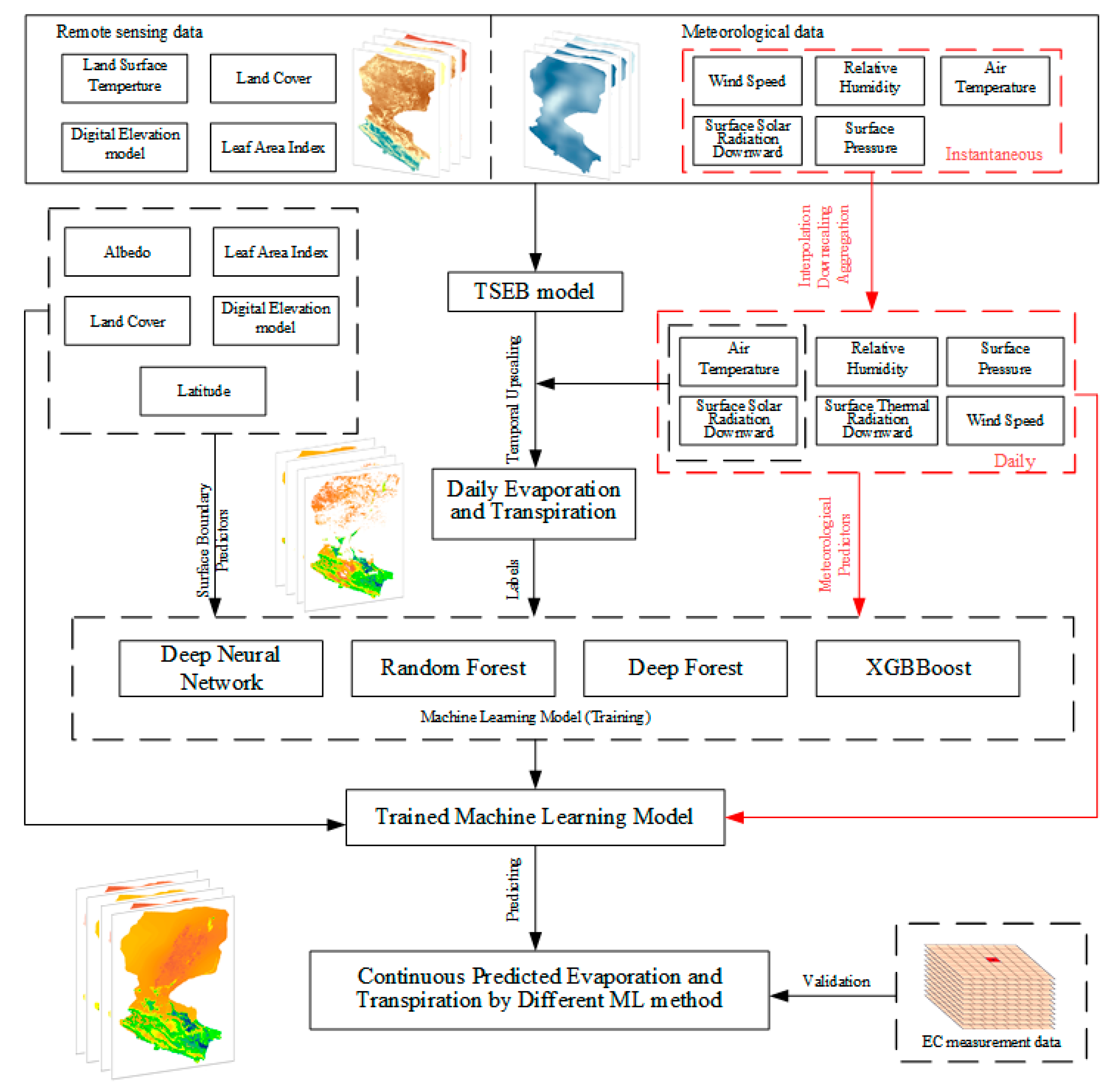
The flowchart for generating spatio-temporal continuous daily ET by the TSEB model and machine learning methods is shown in Figure 2. After the pre-processing of remote sensing and meteorological data was finished, the spatio-temporal discontinuous daily ET was first generated by the TSEB model using remote sensing and instantaneous meteorological data. To reconstruct the gaps in TSEB simulation, four machine learning methods (RF, DNN, DF, XGBoost) were trained and then employed to reconstruct the above gaps in this study. At last, the reconstructed daily ET time series by different machine learning methods were obtained.
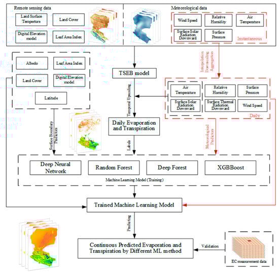
Figure 2.
Flowchart of the estimation and reconstruction of the daily T and E based on TSEB and four machine learning methods. Note that the EC measurement data were used only for accuracy verification.
2.3.1. Description of the TSEB Model
The TSEB model, proposed by Norman in 1995 [6], is a physically based two-source energy balance model used in remote sensing and hydrological studies. The TSEB model can be used to estimate surface energy fluxes at different scales and considers two separate energy components: the soil and the vegetation. It can be applied to accurately estimate the radiative and turbulent energy exchange between the canopy, soil and atmosphere with different vegetation types and climatic areas and has demonstrated robust performances [44,45]. Moreover, the TSEB model is easy to combine with remote sensing, enabling the estimation of evapotranspiration with high spatio-temporal resolution [46]. In this study, the TSEB model was initially utilized to estimate the latent fluxes from the canopy and soil at 14:00 and then temporally upscaled to a daily scale by the evaporative fraction constant (ConEF) method. Details of the TSEB model and ConEF method can be found in relevant articles [23,47,48]. Details of the TSEB model can be found in Supplementary Materials.
2.3.2. Machine Learning Methods for Filling the Gaps
The TSEB model generated gaps in 45.2% of Heihe River Basin due to the cloud cover and the mechanism of TSEB [25]. Machine learning methods can be used to explore and establish complex nonlinear relationships between multiple variables [25,32]. In this study, four machine learning methods (RF, DF, DNN, XGBoost) were employed to reconstruct gaps after TSEB estimation for Heihe River basin. Considering the influence of various factors on ET, surface parameters including LAI, Albedo, LC and meteorological variables including Ta, RH, RH, SSRD, STRD and WS were used to train the machine learning methods. DEM and latitude (LAT) were also employed to further constrain and train the machine learning methods in order to depict the influence of terrain and latitudinal zonation on ET [25].
The trained models combining spatio-temporally continuous parameters were subsequently applied to reconstruct gaps, respectively. The relationship between ET and impact factors can be expressed as follows:
where the represents the nonlinear relationship between and impact factors and the subscript represents different machine learning methods. It should be noted that in order to improve the stability, accelerate the convergence and avoid gradient vanishing or exploding, the inputs of the training parameters were normalized initially.
2.4. SHAP Explanation
The “black-box” nature of machine learning methods is an important feature that refers to the fact that such models are difficult to understand. The SHAP method can indirectly explain the contribution of features to model predictions using the Shapley value. Lundberg and Lee extended the concept of the Shapley value and used it to quantify the contribution of each feature to the model output [49]. SHAP values are calculated based on weighted averages of differences between predictions when training the model with all features and with focused features removed. A larger absolute value of SHAP means that the variables have a greater impact on the retrieval results. In this study, the SHAP value was used to quantify the comprehensive contribution of each parameter to ET.
2.5. Site-Scale Validation
Based on the EC flux data, the daily ETs generated by different machine learning methods were compared with ground measurements to validate the accuracy of them, respectively. In this study, the correlation coefficient (R), bias (unit: mm day−1) and root mean square error (RMSE, unit: mm day−1) were selected as quantitative indicators to evaluate the accuracy of the generated ET, and the expression is as follows:
where and represent the generated and observed daily ET, respectively, the subscript denotes the ith sample, the symbols of and denote the mean of the generated and observed daily ET, and n represents the sample size. A larger R and smaller RMSE and bias indicate better performance; furthermore, the bias can reflect the overall overestimation and underestimation.
2.6. Uncertainty Evaluation at the Regional Scale
Since site-scale validation is not representative of accuracy for the whole basin, the three-cornered hat (TCH) method was employed for cross-validation between daily ETs reconstructed by different machine learning methods. The generalized TCH method can be employed to estimate the relative uncertainty of the ET time series from different reconstruction methods without any ground measurement [50]. The details of the generalized TCH method are described below.
The time series of daily ET can be decomposed into two parts: true value and error:
where all variables are time series, represents the th time series of reconstructed daily ET, is the truth value series, represents the error term of the ith time series and is the number of datasets involved in the calculation. In this study, was 4. In order to calculate the relative uncertainty of each reconstructed ET result, the true value series () needed to be known. But, most of the true values were difficult to observe. Therefore, the TCH method defined the difference between series and reference series () as follows:
where is a matrix with an time series. Since the choice of is theoretically insensitive in the TCH method, it can be randomly selected. DNN reconstructed daily ET was selected as in this study. The covariance matrix of can be obtained using . The unknown covariance matrix of the individual noise is related to :
where is an identity matrix and a is . Because the number of unknown elements is larger than the number of equations, the above equation could not be solved. In order to solve these equations, the constrained minimization problem was proposed by Galindo and Palacio [51] based on the Kuhn–Tucker theorem. Finally, the matrix R was obtained by minimizing the objective function. The uncertainty of the time series () was the square root of the diagonal elements of the matrix and the relative uncertainty was defined as the ratio of the uncertainty to the mean value of each uncertainty.
3. Results
3.1. Determination of Key Input Parameters
In this study, eleven spatio-temporally continuous parameters were employed to train machine learning models and reconstruct daily ET. Correlation coefficient matrix analysis can be used to capture the linear relationships between individual variables and daily ET [52]. The result revealed that LAI had a strong positive correlation with T (R = 0.76) and a weak negative correlation with E (R = −0.14) (Figure 3). This highlighted the crucial role of vegetation in the partitioning of ET as high LAI may impede energy reaching the soil surface. Additionally, the radiation terms SSRD and STRD, as primary energy sources, showed moderate correlations with ET. All other variables showed different linear correlations with ET.

Figure 3.
Pearson correlation coefficient matrix of all parameters. The sample size for the calculation of correlation coefficients was 2189858. All p−values for the correlation coefficients (two−tailed) were less than 0.01.
However, ET is influenced by multiple factors, and interactions among these factors exist. The correlation coefficients may not adequately represent the effects on ET in the actual environment. Therefore, SHAP analysis was introduced in this study to analyze the comprehensive effect of different variables on ET (Figure 4). The SHAP analysis indicated that LAI and SSRD had the greatest effect on ET, with SHAP values of 0.26 and 0.21, respectively. Other parameters also exhibited comparable average impacts. This highlights their influence on the water exchange between the surface and the atmosphere. It is noteworthy that Albedo and RH showed the smallest impact (SHAP values ≈ 0.01) on ET, contrary to the results of the correlation analysis (absolute value of R > 0.3). This discrepancy may be attributed to the SHAP analysis considering interaction effects between features, whereas correlation coefficients only focus on the linear relationships of individual features. The effects of Albedo and relative humidity on ET may be attenuated by other variables.
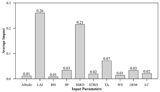
Figure 4.
Average impact values of input parameters calculated by the SHAP method.
Overall, all parameters showed different levels of importance and were involved in the model training and reconstruction.
3.2. Validation of Reconstructed Daily ET
Figure 5, Figure 6, Figure 7 and Figure 8 show the daily ET reconstructed by different machine learning methods compared to ground measurements at the six EC sites. Overall, the generated daily ET (including TSEB-estimated and reconstructed daily ET) demonstrated great and similar performances, with an average R of 0.74, bias between 0.08 and 0.11 mm day−1, and RMSE between 1.11 and 1.15 mmday−1. However, when only the reconstructed daily ET was considered, the discrepancies between different machine learning methods were reflected (Figure 9). Apparently, most points were clustered in the range where ET was less than 2 mm day−1. This phenomenon can be attributed to the fact that lower ET is usually accompanied by lower solar radiation. Under these conditions, LST may not be available and the TSEB model is more likely to fail. As the ET increases, the distribution of points tends to disperse. Despite these discrepancies, the reconstructed ET by different machine learning methods usually showed reasonable accuracy. Among them, the daily ET reconstructed by the XGB model had the highest performance, with an R, bias and RMSE of 0.76, 0.06 mm day−1 and 0.52 mmday−1, followed by the DNN and RF models. On the contrary, the DF model showed slightly worse performance, with R, bias and RMSE of 0.66, 0.04 mm day−1 and 0.55 mm day−1, respectively, and the reconstruction had greater scatter in the lower value range.
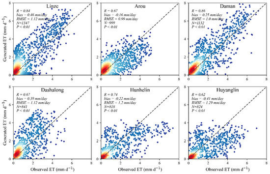
Figure 5.
Validation of generated daily ET (including TSEB−estimated and reconstructed daily ET) using DF at six EC sites. The dashed line is a 1:1 line.
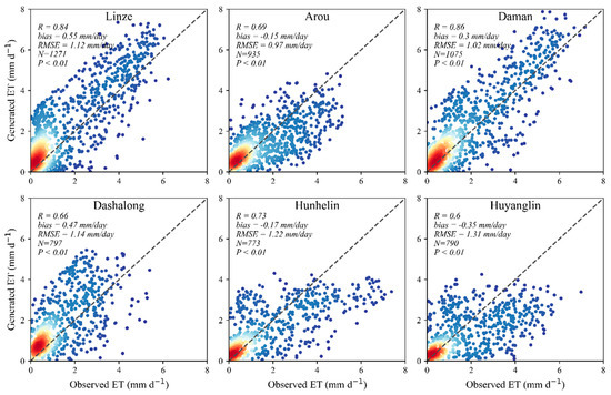
Figure 6.
Validation of generated daily ET (including TSEB−estimated and reconstructed daily ET) using DNN at six EC sites.
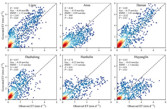
Figure 7.
Validation of generated daily ET (including TSEB−estimated and reconstructed daily ET) using RF at six EC sites.

Figure 8.
Validation of generated daily ET (including TSEB−estimated and reconstructed daily ET) using XGB at six EC sites.
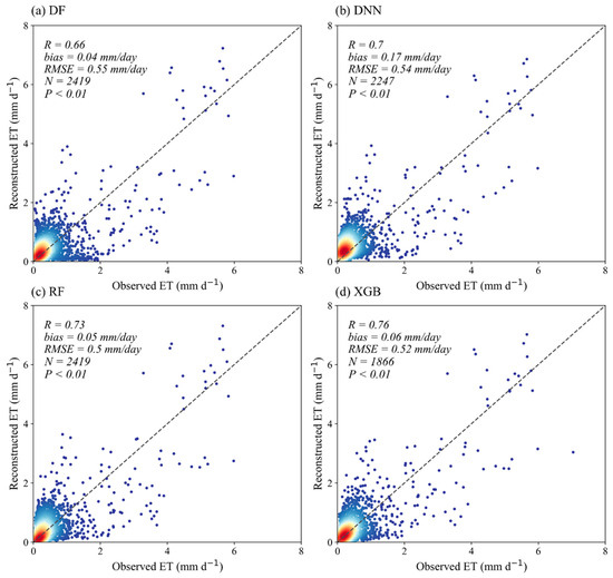
Figure 9.
Validation of reconstructed daily ET by (a) DF, (b) DNN, (c) RF and (d) XGB at EC sites. Only daily ET reconstructed by machine learning methods are considered.
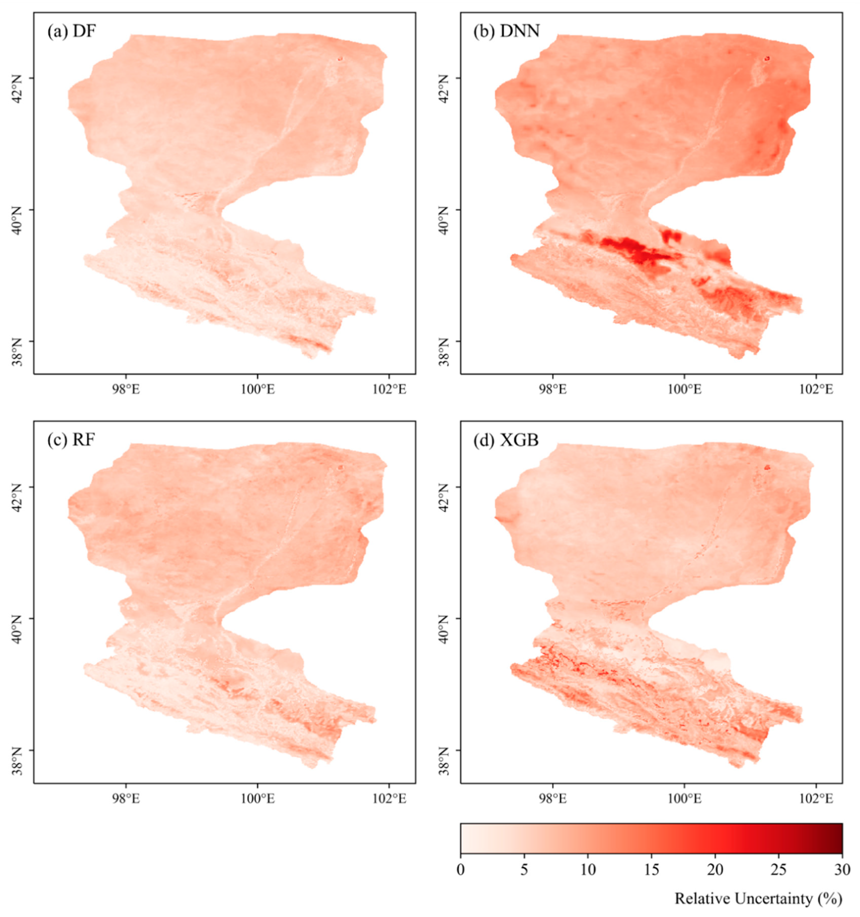
3.3. Relative Uncertainty at the Basin Scale
Direct validation at the site scale does not adequately represent spatial performance. Due to the difficulty of obtaining direct observations at large scales, the TCH method was employed to calculate the relative uncertainty of different machine learning methods in this study. The spatial distributions of relative uncertainty of daily ET reconstructed by different models are shown in Figure 10. Overall, the reconstruction results of all four methods had low relative uncertainty for the whole basin, with average relative uncertainties of 5.36%, 9.35%, 5.95% and 6.44% for DF, DNN, RF and XGB, respectively. However, the DNN model had overall high relative uncertainty, especially for the deserts at the junction between the midstream and upstream regions (>20%). The relative uncertainty of XGB-reconstructed daily ET showed a patchy distribution in the Heihe River region. This may be related to the gaps that remained in these regions after XGB model reconstruction. The DF and RF models, on the other hand, had an analogical distribution of uncertainty across the basin, without significant high values. This could mean that DF and RF are more robust at whole-basin scales.
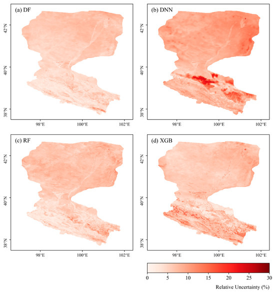
Figure 10.
Spatial distribution of relative uncertainties of daily ET reconstructed by four machine learning methods over Heihe River Basin.
3.4. Spatial Distribution of Reconstructed ET
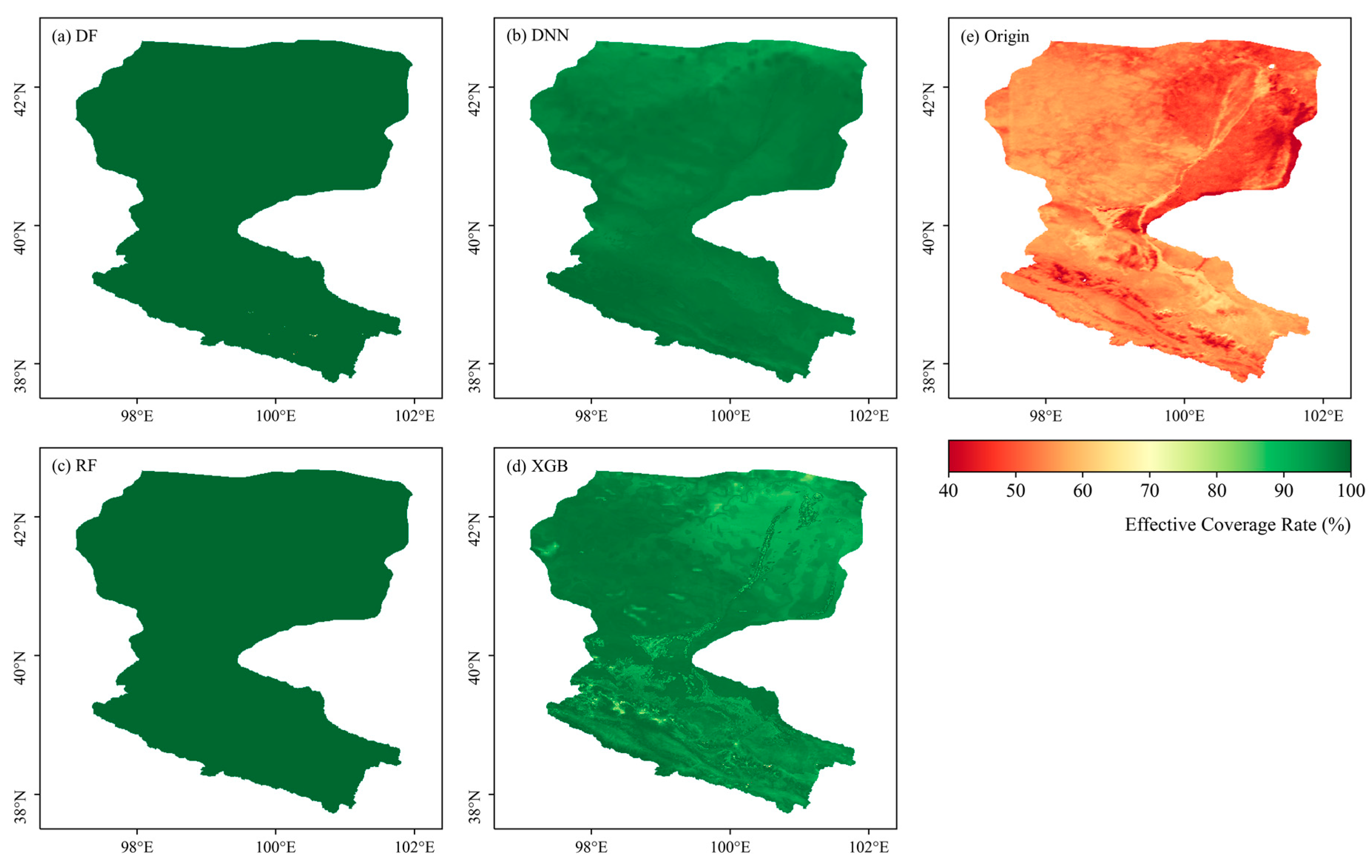
Figure 11 shows cumulative distribution frequency curves vs. effective coverage percentage of the TSEB-estimated and reconstructed daily ET. The areas of the curve on the X-axis in the figure represent the missing amounts. They indicated that RF and DF completely reconstructed the gaps after TSEB estimation, but there remained some gaps when ET was reconstructed by DNN and XGB. In order to further understand the effectiveness of different reconstruction methods, the spatial patterns of the effective coverage rate of daily ET (ratio of the number of days with valid ET against the total days) estimated by these methods and the original TSEB model are shown in Figure 11. The coverage of TSEB model-estimated ET for deserts was lower than for other regions, regardless of the region of the basin. The average effective coverage rates of daily ET after reconstruction with DF, DNN, RF and XGB were improved from 54.8% to 100%, 94.8%, 100% and 94.5%, respectively, for the original TSEB model (Figure 11 and Figure 12). The DNN model exhibited a low coverage rate for the downstream desert regions, while the low coverage rate after XGB-model reconstruction was sporadically distributed throughout the basin.
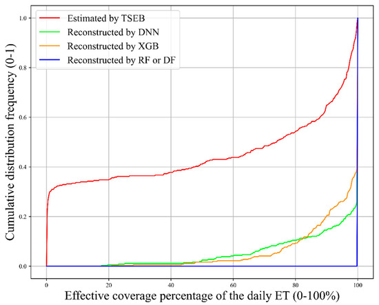
Figure 11.
Plot of cumulative distribution frequency curves vs. effective coverage percentage of the daily ET. The area of the curve on the X−axis in the figure represent the missing amounts. The blue line in the figure indicates that the coverage of daily ET reconstructed by RF or DF was always 100%.
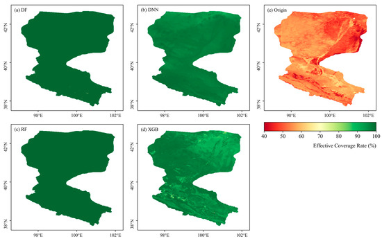
Figure 12.
Temporal coverage of ET estimated from (a–d) different machine learning methods and (e) original TSEB model.
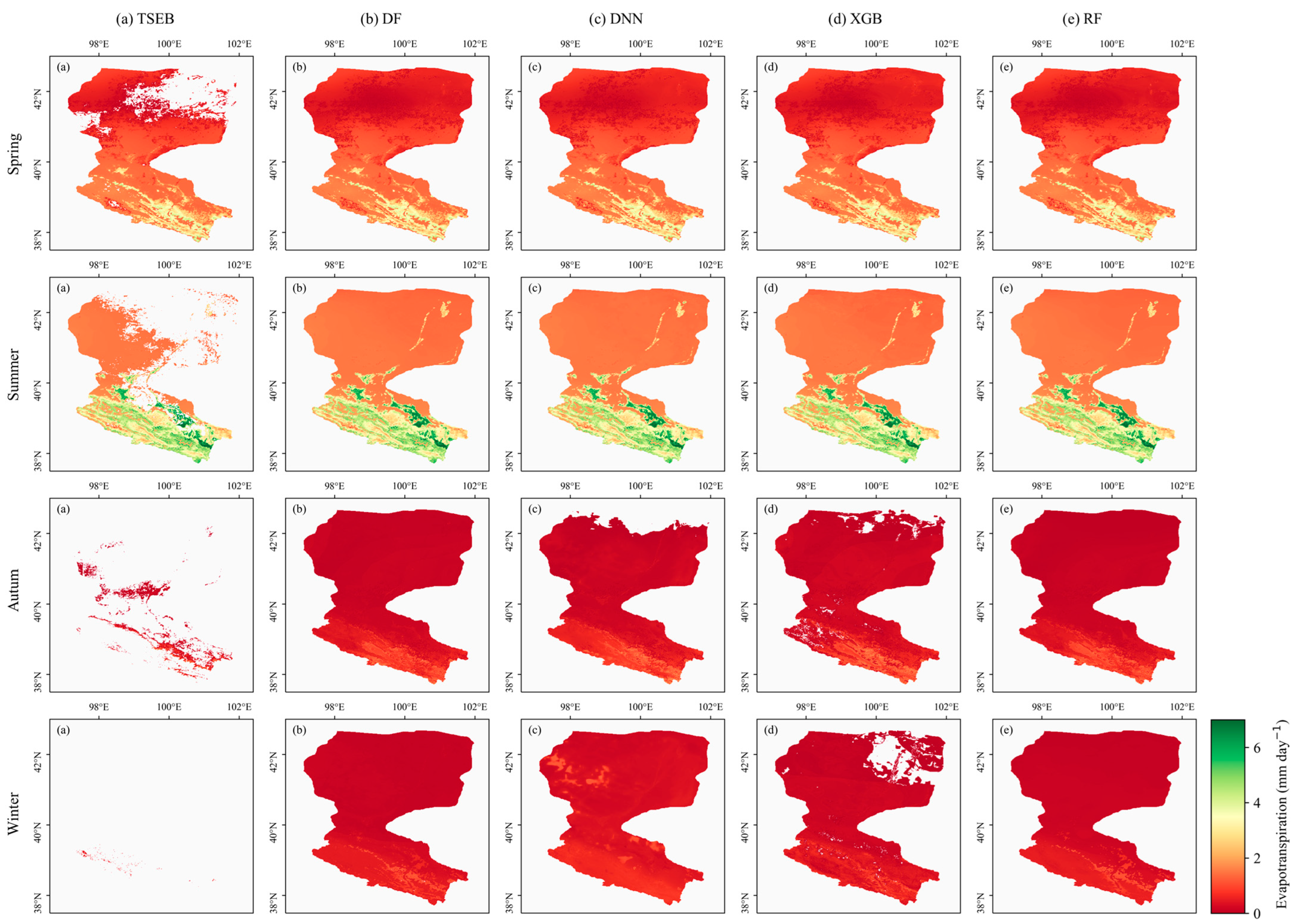
Figure 13 shows the spatial patterns of the TSEB model-estimated and reconstructed daily ET for different seasons. In terms of spatial effectiveness, the TSEB model-estimated ET showed significant gaps in all seasons, particularly in autumn and winter. Additionally, gaps were more prevalent for deserts where daily ET was low (<2 mm day−1). Combined with Figure 10, observing the reconstruction results by different machine learning methods, the DF and RF methods completely reconstructed the daily ET in all seasons, but the DNN and XGB methods showed some localized gaps in winter and autumn. Most of these gaps were more apparent for the desert of the downstream region. Furthermore, the XGB model showed more patchy gaps in the upstream and midstream regions. This suggested that the DNN and XGB models may not be suitable for desert regions.

Figure 13.
Spatial patterns of (a) TSEB-estimated daily ET and daily ET reconstructed by (b) DF, (c) DNN, (d) XGB and (e) RF in different seasons. The white areas represent gaps.
4. Discussion
4.1. Coupling of the TSEB Model and Machine Learning Methods
In this study, the TSEB model-estimated gaps of daily ET maps were reconstructed by using different machine learning methods and multi-source remote sensing data. The results showed that although most of the reconstructed daily ET values were concentrated in the lower range, these low values of daily ET still had an important influence on the hydrological effects of the basin [53]. In addition, the high values of ET in this study also showed reasonable consistency compared to the ground measurements. In previous studies, machine learning methods were widely used mainly to upscale daily ET using ground measurements [36,54]. While this approach may be able to generate spatio-temporally continuous ET at a regional scale, it lacks a reasonable physical explanation [32]. Subsequent studies have employed machine learning methods for reconstruction at a regional scale where LST information is invalid [22,25,55]. In such studies, researchers have trained machine learning methods using the valid outputs of physical models as labels. The models trained in this way not only have the support of the physical theory but can also provide accurate ET estimates without LST information [22,56]. However, previous studies found that the TSEB model and machine learning methods may not yield valid results due to low solar shortwave radiation, even when the LST information is available [25]. The reasons for this phenomenon may be the limitations of the TSEB model itself under low available energy conditions and extreme meteorological conditions [14]. Therefore, this study also explored whether different machine learning methods performed reasonably well in such regions.
4.2. Importance of Input Parameters
The selection of appropriate input variables is crucial before deep learning model training [52]. In the theory of TSEB, ET is constrained not only by surface parameters but also by various meteorological driving factors [14]. Based on this, in this study, Albedo and LC were chosen to represent the effect of land surface character; LAI represented the effect of vegetation and WS, TA, RH, SP, SSRD and STRD represented the effect of atmosphere. Also, considering the latitudinal zonation of ET and topography, DEM and LAT were chosen as key input parameters [25]. However, this study was conducted at a spatial resolution of 0.01°. Given that multiple variables were required for the TSEB model and machine learning methods, we combined input parameters from multiple sources and unified their spatial and temporal resolution to 0.01° and daily by bilinear interpolation. However, this approach to data processing can raise some issues. For instance, the meteorological factors provided by the ERA5-land dataset originally had a spatial resolution of 0.1°, and we downscaled it to 0.01° by bilinear interpolation. However, extreme meteorological conditions and advection are prevalent in Heihe River Basin, which may have resulted in the ERA5-land data with 0.1° resolution failing to accurately reflect the actual meteorological conditions due to smoothing effects during the downscaling [57]. Similarly, the GLASS LAI dataset suffers from a comparable problem. The temporal resolution of GLASS LAI is 8-day. In this study, the LAI data were smoothed to daily by a linear smoothing method. This may have little effect in natural vegetation conditions, but it may not accurately capture sharp changes in LAI caused by crop harvesting in croplands. Currently, the spatial representation of remote sensing remains a major challenge. It is expected that more reliable datasets can be developed in future studies to further develop the application of remote sensing in the estimation of surface parameters.
4.3. Comparison of Different Machine Learning Methods for Reconstruction
To reconstruct the TSEB model-estimated ET, four different machine learning methods were used in this study. Although we anticipated a complete reconstruction of the ET over the whole Heihe River Basin, the XGB and DNN models retained gaps after reconstruction. Despite the high reconstruction accuracy of the XGB and DNN models compared to ground measurements (R > 0.7), these gaps indicated that they still have potential for improvement in the reconstruction of regional ET. The gaps of the DNN model were uniformly distributed in the desert region downstream of Heihe River Basin, while the gaps of the XGB model showed a patchy distribution throughout Heihe River Basin. This phenomenon suggested that the DNN model may have had a more robust performance than the XGB model over the whole basin, even though the accuracy of both models in comparison with ground measurements was comparable. The DF model is a development of the RF model, which has a higher potential in theory. Moreover, the DF model is insensitive to parameter settings [27,31]. However, we found that although the DF model completely reconstructed the daily ET for the whole basin, the DF model had the lowest R value (R = 0.66) compared with ground measurements. The DF model produced numerous low values of daily ET that did not match observations. These issues suggested that the DF model may have limitations in the reconstruction of surface parameters. Summarizing the above comparison, among the four machine learning methods in this study, the RF model had the most robust performance. The RF model not only accomplished the reconstruction of daily ET for Heihe River Basin but also performed well in comparison with ground measurements. Moreover, the RF model had the highest efficiency among the four methods.
In addition, each machine learning method has many parameters to support normal operation. Therefore, the performance of these models may vary significantly with parameter changes [58,59]. However, the focus of this study was to compare their performances in the reconstruction of daily ET. Therefore, the original parameters were not intentionally adjusted here.
5. Conclusions
This study initially drove TSEB to estimate the ET for Heihe River Basin. Subsequently, daily ET was reconstructed using four different machine learning methods (DF, DNN, RF, XGB). At last, the performances of the reconstructed ET from the four machine learning methods were evaluated and compared at site and basin scales. The results showed that the four methods all performed well for Heihe River Basin. The RF model not only demonstrated high prediction accuracy (R = 0.73) but also effectively reconstructed regional ET across all vegetation types, being a more robust model overall. This highlights its suitability as a reliable model for ET reconstruction for Heihe River Basin. The DNN and XGB models achieved high accuracy compared with ground measurements (R > 0.70). However, the reconstructed daily ET retained gaps for the desert region, especially with the XGB model, which had patchy, distributed gaps. The DF model successfully reconstructed daily ET across the whole basin, but it performed poorly (R = 0.66) compared with ground measurements. Moreover, the DF model produced many unreasonable low values. The exploration of this study may provide more references for scholars to estimate or reconstruct ET.
Future research endeavors may enhance the generalizability of these findings by expanding the spatial scale to cover a wider geographic area. Additionally, the integration of other machine learning and physical models presents an opportunity. Combining the strengths of different models may potentially improve the overall accuracy and reliability of ET estimation and reconstruction. These endeavors will contribute to advancing the field of remote sensing-based ET estimation, enabling more robust and versatile applications across diverse environmental contexts.
Supplementary Materials
The following supporting information can be downloaded at: https://www.mdpi.com/article/10.3390/rs16030509/s1, Details of the TSEB Model [6,44,47,60,61,62,63,64].
Author Contributions
This paper is a collaborative work by all of the authors. Conceptualization, G.Z. and L.S.; Data curation, G.Z.; Formal analysis, G.Z.; Methodology, G.Z. and L.S.; Supervision, S.T., L.S., L.Z. and G.Z.; Writing (original draft), G.Z.; Writing (review and editing), G.Z., L.S., S.T. and L.Z. All authors have read and agreed to the published version of the manuscript.
Funding
This work was supported by the National Natural Science Foundation of China (42071298) and the Anhui Province’s University Science Project for Distinguished Young Scholars (2022AH030025).
Data Availability Statement
We gratefully acknowledge each person’s participation in taking the EC measurements and sharing the measured data on platforms of the National Tibetan Plateau Data Center (https://data.tpdc.ac.cn/) and the flux data used in this study was accessed on 10 November 2023.
Acknowledgments
I would like to thank Song Lisheng for his guidance, Tao Sino for his suggestions on revising the paper and Zhao Long for his valuable comments and discussions.
Conflicts of Interest
The authors declare that they have no conflicts of interest to disclose.
References
- Jung, M.; Reichstein, M.; Ciais, P.; Seneviratne, S.I.; Sheffield, J.; Goulden, M.L.; Bonan, G.; Cescatti, A.; Chen, J.Q.; de Jeu, R.; et al. Recent decline in the global land evapotranspiration trend due to limited moisture supply. Nature 2010, 467, 951–954. [Google Scholar] [CrossRef]
- Seneviratne, S.I.; Corti, T.; Davin, E.L.; Hirschi, M.; Jaeger, E.B.; Lehner, I.; Orlowsky, B.; Teuling, A.J. Investigating soil moisture-climate interactions in a changing climate: A review. Earth Sci. Rev. 2010, 99, 125–161. [Google Scholar] [CrossRef]
- Chen, H.; Huang, J.H.J.; McBean, E.; Singh, V.P. Evaluation of alternative two-source remote sensing models in partitioning of land evapotranspiration. J. Hydrol. 2021, 597, 126029. [Google Scholar] [CrossRef]
- Wang, K.C.; Dickinson, R.E. A Review of Global Terrestrial Evapotranspiration: Observation, Modeling, Climatology, and Climatic Variability. Rev. Geophys. 2012, 50, RG2005. [Google Scholar] [CrossRef]
- Liu, S.M.; Xu, Z.W.; Song, L.S.; Zhao, Q.Y.; Ge, Y.; Xu, T.R.; Ma, Y.F.; Zhu, Z.L.; Jia, Z.Z.; Zhang, F. Upscaling evapotranspiration measurements from multi-site to the satellite pixel scale over heterogeneous land surfaces. Agric. For. Meteorol. 2016, 230, 97–113. [Google Scholar] [CrossRef]
- Norman, J.M.; Kustas, W.P.; Humes, K.S. Source Approach for Estimating Soil and Vegetation Energy Fluxes in Observations of Directional Radiometric Surface-Temperature. Agric. Forest Meteorol. 1995, 77, 263–293. [Google Scholar] [CrossRef]
- Norman, J.M.; Kustas, W.P.; Prueger, J.H.; Diak, G.R. Surface flux estimation using radiometric temperature: A dual temperature-difference method to minimize measurement errors. Water Resour. Res. 2000, 36, 2263–2274. [Google Scholar] [CrossRef]
- Penman, H.L. Natural Evaporation from Open Water, Bare Soil and Grass. Proc. R. Soc. Lond. Ser. A Math. Phys. Sci. 1948, 193, 120–145. [Google Scholar] [CrossRef]
- Leuning, R.; Zhang, Y.Q.; Rajaud, A.; Cleugh, H.; Tu, K. A simple surface conductance model to estimate regional evaporation using MODIS leaf area index and the Penman-Monteith equation. Water Resour. Res. 2008, 44, W10419. [Google Scholar] [CrossRef]
- Zhang, Y.Q.; Leuning, R.; Hutley, L.B.; Beringer, J.; McHugh, I.; Walker, J.P. Using long-term water balances to parameterize surface conductances and calculate evaporation at 0.05 degrees spatial resolution. Water Resour. Res. 2010, 46, W05512. [Google Scholar] [CrossRef]
- Bastiaanssen, W.G.M.; Menenti, M.; Feddes, R.A.; Holtslag, A.A.M. A remote sensing surface energy balance algorithm for land (SEBAL)–1. Formulation. J. Hydrol. 1998, 212, 198–212. [Google Scholar] [CrossRef]
- Chen, J.M.; Liu, J. Evolution of evapotranspiration models using thermal and shortwave remote sensing data. Remote Sens. Environ. 2020, 237, 111594. [Google Scholar] [CrossRef]
- Song, L.S.; Ding, Z.H.; Kustas, W.P.; Xu, Y.H.; Zhao, G.; Liu, S.M.; Ma, M.G.; Xue, K.J.; Bai, Y.; Xu, Z.W. Applications of a thermal-based two-source energy balance model coupled to surface soil moisture. Remote Sens. Environ. 2022, 271, 112923. [Google Scholar] [CrossRef]
- Song, L.S.; Kustas, W.P.; Liu, S.M.; Colaizzi, P.D.; Nieto, H.; Xu, Z.W.; Ma, Y.F.; Li, M.S.; Xu, T.R.; Agam, N.; et al. Applications of a thermal-based two-source energy balance model using Priestley-Taylor approach for surface temperature partitioning under advective conditions. J. Hydrol. 2016, 540, 574–587. [Google Scholar] [CrossRef]
- Xu, Y.H.; Song, L.S.; Kustas, W.P.; Xue, K.J.; Liu, S.M.; Ma, M.G.; Xu, T.R.; Zhao, L. Application of the two-source energy balance model with microwave-derived soil moisture in a semi-arid agricultural region. Int. J. Appl. Earth Obs. 2022, 112, 102879. [Google Scholar] [CrossRef]
- Knipper, K.; Yang, Y.; Anderson, M.; Bambach, N.; Kustas, W.; McElrone, A.; Gao, F.; Alsina, M.M. Decreased latency in landsat-derived land surface temperature products: A case for near-real-time evapotranspiration estimation in California. Agric. Water Manag. 2023, 283, 108316. [Google Scholar] [CrossRef]
- Li, Y.; Huang, C.L.; Kustas, W.P.; Nieto, H.; Sun, L.; Hou, J.L. Evapotranspiration Partitioning at Field Scales Using TSEB and Multi-Satellite Data Fusion in The Middle Reaches of Heihe River Basin, Northwest China. Remote Sens. 2020, 12, 3223. [Google Scholar] [CrossRef]
- Guzinski, R.; Nieto, H.; Sandholt, I.; Karamitilios, G. Modelling High-Resolution Actual Evapotranspiration through Sentinel-2 and Sentinel-3 Data Fusion. Remote Sens. 2020, 12, 1433. [Google Scholar] [CrossRef]
- Feng, J.J.; Wang, W.Z.; Che, T.; Xu, F.A. Performance of the improved two-source energy balance model for estimating evapotranspiration over the heterogeneous surface. Agric. Water Manag. 2023, 278, 108159. [Google Scholar] [CrossRef]
- Amjad, M.; Yilmaz, M.T.; Yucel, I.; Yilmaz, K.K. Performance evaluation of satellite- and model-based precipitation products over varying climate and complex topography. J. Hydrol. 2020, 584, 124707. [Google Scholar] [CrossRef]
- Muñoz-Sabater, J.; Dutra, E.; Agustí-Panareda, A.; Albergel, C.; Arduini, G.; Balsamo, G.; Boussetta, S.; Choulga, M.; Harrigan, S.; Hersbach, H.; et al. ERA5-Land: A state-of-the-art global reanalysis dataset for land applications. Earth Syst. Sci. Data 2021, 13, 4349–4383. [Google Scholar] [CrossRef]
- Song, L.S.; Bateni, S.M.; Xu, Y.H.; Xu, T.R.; He, X.L.; Ki, S.J.; Liu, S.M.; Ma, M.G.; Yang, Y. Reconstruction of remotely sensed daily evapotranspiration data in cloudy-sky conditions. Agric. Water Manag. 2021, 255, 107000. [Google Scholar] [CrossRef]
- Xu, T.; Liu, S.; Xu, L.; Chen, Y.; Jia, Z.; Xu, Z.; Nielson, J. Temporal Upscaling and Reconstruction of Thermal Remotely Sensed Instantaneous Evapotranspiration. Remote Sens. 2015, 7, 3400–3425. [Google Scholar] [CrossRef]
- Jiang, Y.Z.; Tang, R.L.; Li, Z.L. Reconstruction of daily evapotranspiration under cloudy sky constrained by soil water budget balance. J. Hydrol. 2022, 605, 127288. [Google Scholar] [CrossRef]
- Cui, Y.K.; Song, L.S.; Fan, W.J. Generation of spatio-temporally continuous evapotranspiration and its components by coupling a two-source energy balance model and a deep neural network over the Heihe River Basin. J. Hydrol. 2021, 597, 126176. [Google Scholar] [CrossRef]
- Breiman, L. Random forests. Mach. Learn. 2001, 45, 5–32. [Google Scholar] [CrossRef]
- Zhou, Z.H.; Feng, J. Deep forest. Natl. Sci. Rev. 2019, 6, 74–86. [Google Scholar] [CrossRef] [PubMed]
- Chen, T.; Guestrin, C. XGBoost: A Scalable Tree Boosting System; ACM: New York, NY, USA, 2016. [Google Scholar]
- Agrawal, Y.; Kumar, M.; Ananthakrishnan, S.; Kumarapuram, G. Evapotranspiration Modeling Using Different Tree Based Ensembled Machine Learning Algorithm. Water Resour. Manag. 2022, 36, 1025–1042. [Google Scholar] [CrossRef]
- Chatterjee, S.; Kandiah, R.; Watts, D.; Sritharan, S.; Osterberg, J. Estimating Completely Remote Sensing-Based Evapotranspiration for Salt Cedar (Tamarix ramosissima), in the Southwestern United States, Using Machine Learning Algorithms. Remote Sens. 2023, 15, 5021. [Google Scholar] [CrossRef]
- Li, M.Y.; Yang, Q.Q.; Yuan, Q.Q.; Zhu, L.Y. Estimation of high spatial resolution ground-level ozone concentrations based on Landsat 8 TIR bands with deep forest model. Chemosphere 2022, 301, 134817. [Google Scholar] [CrossRef]
- Yuan, Q.Q.; Shen, H.F.; Li, T.W.; Li, Z.W.; Li, S.W.; Jiang, Y.; Xu, H.Z.; Tan, W.W.; Yang, Q.Q.; Wang, J.W.; et al. Deep learning in environmental remote sensing: Achievements and challenges. Remote Sens. Environ. 2020, 241, 111716. [Google Scholar] [CrossRef]
- Duan, S.B.; Lian, Y.H.; Zhao, E.Y.; Chen, H.; Han, W.J.; Wu, Z.H. A Novel Approach to All-Weather LST Estimation Using XGBoost Model and Multisource Data. IEEE Trans. Geosci. Remote 2023, 61, 5004614. [Google Scholar] [CrossRef]
- Yu, T.; Zhang, Q.; Sun, R. Comparison of Machine Learning Methods to Up-Scale Gross Primary Production. Remote Sens. 2021, 13, 2448. [Google Scholar] [CrossRef]
- Li, Q.L.; Shi, G.S.; Shangguan, W.; Nourani, V.; Li, J.D.; Li, L.; Huang, F.N.; Zhang, Y.; Wang, C.Y.; Wang, D.G.; et al. A 1 km daily soil moisture dataset over China using in situ measurement and machine learning. Earth Syst. Sci. Data 2022, 14, 5267–5286. [Google Scholar] [CrossRef]
- Xu, T.R.; Guo, Z.X.; Liu, S.M.; He, X.L.; Meng, Y.F.Y.; Xu, Z.W.; Xia, Y.L.; Xiao, J.F.; Zhang, Y.; Ma, Y.F.; et al. Evaluating Diffferent Machine Learning Methods for Upscaling Evapotranspiration from Flux Towers to the Regional Scale. J. Geophys. Res. Atmos. 2018, 123, 8674–8690. [Google Scholar] [CrossRef]
- Cheng, G.D.; Li, X.; Zhao, W.Z.; Xu, Z.M.; Feng, Q.; Xiao, S.C.; Xiao, H.L. Integrated study of the water-ecosystem-economy in the Heihe River Basin. Natl. Sci. Rev. 2014, 1, 413–428. [Google Scholar] [CrossRef]
- Li, X.; Cheng, G.D.; Liu, S.M.; Xiao, Q.; Ma, M.G.; Jin, R.; Che, T.; Liu, Q.H.; Wang, W.Z.; Qi, Y.; et al. Heihe Watershed Allied Telemetry Experimental Research (HiWATER): Scientific Objectives and Experimental Design. Bull. Am. Meteorol. Soc. 2013, 94, 1145–1160. [Google Scholar] [CrossRef]
- Liu, S.M.; Li, X.; Xu, Z.W.; Che, T.; Xiao, Q.; Ma, M.G.; Liu, Q.H.; Jin, R.; Guo, J.W.; Wang, L.X.; et al. The Heihe Integrated Observatory Network: A Basin-Scale Land Surface Processes Observatory in China. Vadose Zone J. 2018, 17, 180072. [Google Scholar] [CrossRef]
- Ji, X.B.; Zhao, W.Z.; Jin, B.W.; Zhao, L.W.; Zhao, W.Y.; Du, Z.Y.; Chen, Z.; Zhang, L.M. A dataset of water, heat, and carbon fluxes of an oasis agroecosystem in the middle areas of the Hexi Corridor (2012–2015). China Sci. Data 2023, 8. [Google Scholar] [CrossRef]
- Zhang, X.D.; Zhou, J.; Liang, S.L.; Wang, D.D. A practical reanalysis data and thermal infrared remote sensing data merging (RTM) method for reconstruction of a 1-km all-weather land surface temperature. Remote Sens. Environ. 2021, 260, 112437. [Google Scholar] [CrossRef]
- Liang, S.L.; Zhao, X.; Liu, S.H.; Yuan, W.P.; Cheng, X.; Xiao, Z.Q.; Zhang, X.T.; Liu, Q.; Cheng, J.; Tang, H.R.; et al. A long-term Global LAnd Surface Satellite (GLASS) data-set for environmental studies. Int. J. Digit. Earth 2013, 6, 5–33. [Google Scholar] [CrossRef]
- Sulla-Menashe, D.; Gray, J.M.; Abercrombie, S.P.; Friedl, M.A. Hierarchical mapping of annual global land cover 2001 to present: The MODIS Collection 6 Land Cover product. Remote Sens. Environ. 2019, 222, 183–194. [Google Scholar] [CrossRef]
- Kustas, W.P.; Norman, J.M. A two-source energy balance approach using directional radiometric temperature observations for sparse canopy covered surfaces. Agron. J. 2000, 92, 847–854. [Google Scholar] [CrossRef]
- Burchard-Levine, V.; Nieto, H.; Riano, D.; Kustas, W.P.; Migliavacca, M.; El-Madany, T.S.; Nelson, J.A.; Andreu, A.; Carrara, A.; Beringer, J.; et al. A remote sensing-based three-source energy balance model to improve global estimations of evapotranspiration in semi-arid tree-grass ecosystems. Glob. Change Biol. 2022, 28, 1493–1515. [Google Scholar] [CrossRef]
- Jaafar, H.H.; Mourad, R.M.; Kustas, W.P.; Anderson, M.C. A Global Implementation of Single- and Dual-Source Surface Energy Balance Models for Estimating Actual Evapotranspiration at 30-m Resolution Using Google Earth Engine. Water Resour. Res. 2022, 58, e2022WR032800. [Google Scholar] [CrossRef]
- Kustas, W.P.; Alfieri, J.G.; Nieto, H.; Wilson, T.G.; Gao, F.; Anderson, M.C. Utility of the two-source energy balance (TSEB) model in vine and interrow flux partitioning over the growing season. Irrig. Sci. 2019, 37, 375–388. [Google Scholar] [CrossRef]
- Cammalleri, C.; Anderson, M.C.; Kustas, A.P. Upscaling of evapotranspiration fluxes from instantaneous to daytime scales for thermal remote sensing applications. Hydrol. Earth Syst. Sci. 2014, 18, 1885–1894. [Google Scholar] [CrossRef]
- Lundberg, S.; Lee, S.I. A Unified Approach to Interpreting Model Predictions. In Proceedings of the Thirty-first Annual Conference on Neural Information Processing Systems (NIPS), Long Beach, CA, USA, 4–9 December 2017. [Google Scholar]
- Liu, J.; Chai, L.N.; Dong, J.Z.; Zheng, D.H.; Wigneron, J.P.; Liu, S.M.; Zhou, J.; Xu, T.R.; Yang, S.Q.; Song, Y.Z.; et al. Uncertainty analysis of eleven multisource soil moisture products in the third pole environment based on the three-corned hat method. Remote Sens. Environ. 2021, 255, 112225. [Google Scholar] [CrossRef]
- Galindo, F.J.; Palacio, J. Estimating the Instabilities of N Correlated Clocks. Metrologia 1999, 30, 479. [Google Scholar]
- Qin, Z.L.; Zhou, X.Y.; Li, M.Y.; Tong, Y.X.; Luo, H.X. Landslide Susceptibility Mapping Based on Resampling Method and FR-CNN: A Case Study of Changdu. Land 2023, 12, 1213. [Google Scholar] [CrossRef]
- Xue, B.L.; Wang, L.; Li, X.P.; Yang, K.; Chen, D.L.; Sun, L.T. Evaluation of evapotranspiration estimates for two river basins on the Tibetan Plateau by a water balance method. J. Hydrol. 2013, 492, 290–297. [Google Scholar] [CrossRef]
- Zhang, C.Y.; Brodylo, D.; Rahman, M.; Rahman, M.A.; Douglas, T.A.; Comas, X. Using an object-based machine learning ensemble approach to upscale evapotranspiration measured from eddy covariance towers in a subtropical wetland. Sci. Total Environ. 2022, 831, 154969. [Google Scholar] [CrossRef] [PubMed]
- Song, L.S.; Liu, S.M.; Kustas, W.P.; Nieto, H.; Sun, L.; Xu, Z.W.; Skaggs, T.H.; Yang, Y.; Ma, M.G.; Xu, T.R.; et al. Monitoring and validating spatially and temporally continuous daily evaporation and transpiration at river basin scale. Remote Sens. Environ. 2018, 219, 72–88. [Google Scholar] [CrossRef]
- Liang, X.G.; Song, C.Q.; Liu, K.; Chen, T.; Fan, C.Y. Reconstructing Centennial-Scale Water Level of Large Pan-Arctic Lakes Using Machine Learning Methods. J. Earth Sci. China 2023, 34, 1218–1230. [Google Scholar] [CrossRef]
- Gao, H.R.; Zhang, Z.J.; Zhang, W.C.; Chen, H.; Xi, M.J. Spatial Downscaling Based on Spectrum Analysis for Soil Freeze/Thaw Status Retrieved from Passive Microwave. IEEE Trans. Geosci. Remote 2022, 60, 4300211. [Google Scholar] [CrossRef]
- Oliveira, A.L.I.; Braga, P.L.; Lima, R.M.F.; Cornélio, M.L. GA-based method for feature selection and parameters optimization for machine learning regression applied to software effort estimation. Inf. Softw. Technol. 2010, 52, 1155–1166. [Google Scholar] [CrossRef]
- Zuo, X.; Guo, H.; Shi, S.Y.; Zhang, X.C. Comparison of Six Machine Learning Methods for Estimating PM2.5 Concentration Using the Himawari-8 Aerosol Optical Depth. J. Indian Soc. Remote 2020, 48, 1277–1287. [Google Scholar] [CrossRef]
- Kustas, W.P.; Norman, J.M. Evaluation of soil and vegetation heat flux predictions using a simple two-source model with radiometric temperatures for partial canopy cover. Agr. Forest Meteorol. 1999, 94, 13–29. [Google Scholar] [CrossRef]
- Campbell, G.S.; Norman, J.M. An Introduction to Environmental Biophysics; Springer Science & Business Media: Berlin/Heidelberg, Germany, 2000. [Google Scholar]
- Santanello, J.A.; Friedl, M.A. Diurnal covariation in soil heat flux and net radiation. J. Appl. Meteorol. 2003, 42, 851–862. [Google Scholar] [CrossRef]
- Colaizzi, P.D.; Kustas, W.P.; Anderson, M.C.; Agam, N.; Tolk, J.A.; Evett, S.R.; Howell, T.A.; Gowda, P.H.; O’Shaughnessy, S.A. Two-source energy balance model estimates of evapotranspiration using component and composite surface temperatures. Adv. Water Resour. 2012, 50, 134–151. [Google Scholar] [CrossRef]
- Priestley, C.H.B.; Taylor, R.J. Assessment of Surface Heat-Flux and Evaporation Using Large-Scale Parameters. Mon. Weather Rev. 1972, 100, 81. [Google Scholar] [CrossRef]


Disclaimer/Publisher’s Note: The statements, opinions and data contained in all publications are solely those of the individual author(s) and contributor(s) and not of MDPI and/or the editor(s). MDPI and/or the editor(s) disclaim responsibility for any injury to people or property resulting from any ideas, methods, instructions or products referred to in the content. |
© 2024 by the authors. Licensee MDPI, Basel, Switzerland. This article is an open access article distributed under the terms and conditions of the Creative Commons Attribution (CC BY) license (https://creativecommons.org/licenses/by/4.0/).